


Policy Significance Statement
Causal machine learning is beginning to be used in analysis that informs public policy. Particular techniques which estimate individual or group-level effects of interventions are the focus of this article. The article identifies two problems with applying causal machine learning to policy analysis—usability and accountability issues, both of which require greater transparency in models. It argues that some existing tools can help to address these challenges but that users need to be aware of transparency issues and address them to the extent they can using the techniques in this article. To the extent they cannot address issues, users need to decide whether more powerful estimation is really worth less transparency.
1. Introduction
Causal machine learning is currently experiencing a surge of interest as a tool for policy evaluation (Çağlayan Akay et al., Reference Çağlayan Akay, Yılmaz Soydan and Kocarık Gacar2022; Lechner, Reference Lechner2023). With this enthusiasm and maturing of methods, we are likely to see more research using these methods that affect policy decisions. The promise of causal machine learning is that researchers performing causal estimation will be able to take advantage of machine learning models that have previously only been available to predictive modelers (Athey and Imbens, Reference Athey and Imbens2017; Daoud and Dubhashi, Reference Daoud and Dubhashi2020; Baiardi and Naghi, Reference Baiardi and Naghi2021; Imbens and Athey, Reference Imbens and Athey2021). Where traditional (supervised) predictive machine learning aims to estimate outcomes, causal machine learning aims to estimate treatment effects (the difference between an observed outcome for prediction and one which is fundamentally unobservable) for causal modeling as the treatment effect will always be a function of an unobserved potential outcome (Imbens and Rubin, Reference Imbens and Rubin2015). This generally means either plugging standard machine learning models into a special causal estimator or modifying machine learning methods to give causal estimates with good statistical properties (particularly asymptotic normality and consistency). This allows researchers to capture complex functional forms in high-dimensional data which relate cause to effect (Chernozhukov et al., Reference Chernozhukov, Chetverikov, Demirer, Duflo, Hansen, Newey and Robins2018; Knaus, Reference Knaus2022) and allows for a data-driven approach to estimate heterogeneous treatment effects that does not require explicitly including interactions with treatment (Wager and Athey, Reference Wager and Athey2018; Athey et al., Reference Athey, Tibshirani and Wager2019). A good non-technical introduction to this literature can be found in Lechner (Reference Lechner2023).Footnote 1
There seems to be substantial benefits to using causal machine learning when the appropriate methods are applied correctly to the right research project. However, the fact that these methods generally use black-box models makes them very different from traditional causal estimation models. A model being “black-box” means that it is not possible to get a general explanation of how a model arrived at an estimate (Rudin, Reference Rudin2019). For example, in a linear regression, we can easily see how each coefficient multiplied by the data then summed gives a prediction, but in a model like a random forest, we need to understand the average result of potentially thousands of individual decision trees which is practically impossible. A black-box model then is one where we lack a reasonable general explanation of the functioning of the model, instead all that we can find are local explanations for how a particular prediction was made (later we will call this explainable AI [XAI]; Xu et al., Reference Xu, Uszkoreit, Du, Fan, Zhao, Zhu, Tang, Kan, Zhao, Li and Zan2019) or abandon the method and simplify to a “white-box” model like a single decision tree (what we will later call interpretable AI [IAI]; Rudin, Reference Rudin2019). This lack of a general explanation presents challenges when using causal machine learning methods to inform decision-making.
The focus of this article will be on transparency in the case of heterogeneous treatment effect analysis in policy evaluation. By transparency we mean an ability to get useful information about the workings of a black-box model. Specifically we focus on the causal forest method (Wager and Athey, Reference Wager and Athey2018; Athey et al., Reference Athey, Tibshirani and Wager2019). We identify two kinds of transparency that are important, but which need to be thought of separately. These are termed accountability and usability. This classification of types of transparency is orthogonal to the means we might use to achieve transparency such as through XAI and IAI methods and in the latter half of this article we discuss both types of methods as means for achieving both goals.
Accountability is transparency for those who will be subject to policy. Their interest in understanding the analysis used in policy-making is close to the classic case for transparency in predictive machine learning (see Ireni Saban and Sherman, Reference Ireni Saban and Sherman2022 for an introduction to the literature on ethical issues around predictive machine learning and government). A party subject to the decisions made by a model might be owed an explanation for the decisions made and the ability to identify and criticize injustices such as the right codified into the European Union’s GDPR (Kim and Routledge, Reference Kim and Routledge2022). Specifically, transparency with an accountability goal is often concerned with addressing similar problems to machine learning fairness, though through the means of transparency rather than the often blunter means of fairness rules (Rai, Reference Rai2020). This means that accountability concerns are often particularly focused on the use of sensitive variables like gender or race in models. However, this analogy to the predictive case is complicated somewhat by the role of the human decision-maker who is generally interpreting the results of a causal machine learning analysis and making decisions based on it (Rehill and Biddle, Reference Rehill and Biddle2023). Causal machine learning models would rarely make decisions directly as they might in predictive applications, but instead inform a longer policy-making process. It is necessary then to understand the output of a model, but it is also necessary to understand the human decision-making process that was informed by the output and which led to a policy outcome.
Usability is transparency that helps the analyst and decision-maker to understand the data generating process (DGP) and therefore obtain better insights into the causal processes at play. It can also help to diagnose problems in modeling, for example, finding variables that are “bad controls” (Hünermund et al., Reference Hünermund, Kaminski and Schmitt2021) that should not be in the dataset. As with accountability, the primary difference between causal and predictive applications from a justice perspective is not the actual differences in estimation processes, but rather it is the way that causal models are generally there to inform human decision-makers while predictive ones generally exercise more direct power (Rehill and Biddle, Reference Rehill and Biddle2023). Usability is precisely the way in which models do this informing, taking a model of hundreds of thousands of parameters in the case of a typical causal forest and presenting the patterns in those parameters in a way that can tell the user about the underlying causal effects. Because usability is so directly tied to the human role, there is less of a parallel here to the existing transparency literature than there is in accountability but we will explore how existing transparency tools can still be useful for improving usability.
This article is an effort to lay out the problems posed by applying black-box models to causal inference where methods have generally been interpretable in the past. There is little existing literature in this area (we are not familiar with any aside from Gur Ali, Reference Gur Ali2022), however the critical literature around predictive learning provides a blueprint for understanding these concerns and trying to solve them. Section 2 provides a background on causal machine learning. Section 3 explains why these methods might be useful for policy-making. Section 4 looks specifically at transparency in causal machine learning and the role of accountability and usability. Section 5 introduces the case study that will motivate the rest of the article, a study of returns on education in Australia using the Household Income and Labour Dynamics in Australia Survey (HILDA). Section 6 then demonstrates and discusses some possible approaches including XAI, IAI, and refutation tests which can all offer some insight into the causal effects and therefore help inform policy decisions.
2. A brief introduction to causal machine learning
What fundamentally separates causal machine learning from the more typically discussed predictive machine learning is that the latter is concerned with predicting outcomes while the former is concerned with predicting treatment effects. The standard definition of a treatment effect in econometrics relies on the Potential Outcomes (PO) Framework (Imbens and Rubin, Reference Imbens and Rubin2015). For a vector of outcomes
 $ Y $
and a vector of binary treatment assignments
$ Y $
and a vector of binary treatment assignments
 $ W $
, the treatment effect (
$ W $
, the treatment effect (
 $ {\tau}_i $
) is the difference between the potential outcomes as a function of treatment status
$ {\tau}_i $
) is the difference between the potential outcomes as a function of treatment status
 $ {Y}_i\left({W}_i\right) $
 $$ {\tau}_i={Y}_i(1)-{Y}_i(0). $$
There is an obvious problem here, that one cannot both treat and not treat a unit at a given point in time so in effect, we have to impute counterfactual potential outcomes to do causal inference. This is called the “Fundamental Problem of Causal Inference” (Holland, Reference Holland1986). It means that unlike for predictive machine learning, in real world data we lack ground-truth treatment effects on which to train a model. It also means that we are relying on a series of causal assumptions the two key ones being the Stable Unit Treatment Value Assumption (SUTVA), and the Independence Assumption (Imbens and Rubin, Reference Imbens and Rubin2015). The Independence Assumption is required for a causal effect to be considered identified. Essentially it means assuming that treatment assignment is exogenous (as in an experiment), partially exogenous (as in an instrumental variables approach) or endogenous but we will model out the endogeneity for example with a set of control variables (as in control-on-observables) or additional assumptions (as in a difference-in-differences design).
In parametric modeling—given identifying assumptions hold and a linear parameterisation of the relationship is appropriate—it is easy to model causal effects by fitting outcomes. In causal machine learning, predictive methods need to be adapted as regularization shrinks the estimated effect of individual variables toward zero (Chernozhukov et al., Reference Chernozhukov, Chetverikov, Demirer, Duflo, Hansen, Newey and Robins2018). This can be achieved either through specific methods designed to give asymptotically unbiased causal estimates, for example, the causal tree (Athey and Imbens, Reference Athey and Imbens2016) or generic estimators designed to plug in estimates from arbitrary machine learning methods, for example, meta-learners (Künzel et al., Reference Künzel, Sekhon, Bickel and Yu2019; Nie and Wager, Reference Nie and Wager2021). In all these cases though, the methods still do not have access to ground-truth treatment effects and still require SUTVA and independence assumptions meaning that the exercise is not simply one of maximizing fit on held-out data.
Causal machine learning is a broad term for several different families of methods which all draw inspiration from machine learning literature in computer science. One of the most widely-used methods here and our focus for this article is the causal forest (Wager and Athey, Reference Wager and Athey2018; Athey et al., Reference Athey, Tibshirani and Wager2019) which uses a random forest made up of debiased decision trees to minimize the R-loss objective (Nie and Wager, Reference Nie and Wager2021) in order to estimate HTEs (generally after double machine learning is applied for local centering). The causal forest (at least as implemented in the generalized random forest paper and companion R package grf) consists of three key parts, local centering, finding kernel weights and then plug-in estimation.
Local centering removes selection effects in the data (assuming we meet the assumptions of control-on-observables identification) by estimating nuisance parameters using two nuisance models, an estimate of the outcome
 $ m(x)=\unicode{x1D53C}\left[Y|X=x\right] $
and an estimate of the propensity score
$ m(x)=\unicode{x1D53C}\left[Y|X=x\right] $
and an estimate of the propensity score
 $ e(x)=\mathrm{\mathbb{P}}\left[W=1|X=x\right] $
or in the continuous case where we estimate an average partial effect,
$ e(x)=\mathrm{\mathbb{P}}\left[W=1|X=x\right] $
or in the continuous case where we estimate an average partial effect,
 $ e(x)=\unicode{x1D53C}\left[W|X=x\right] $
. (Athey et al., Reference Athey, Tibshirani and Wager2019).Footnote
2 The term nuisance here means that the parameters themselves are not the target of the analysis, but are necessary for estimation of the actual quantity of interest, a treatment effect. This local centering is similar to the double machine learning method which is a popular approach to average treatment effect estimation (Chernozhukov et al., Reference Chernozhukov, Chetverikov, Demirer, Duflo, Hansen, Newey and Robins2018). These models can use arbitrary machine learning methods so long as predictions are not made on data used to train the nuisance model (this is in order to meet regularity conditions in semi-parametric estimation (Chernozhukov et al., Reference Chernozhukov, Chetverikov, Demirer, Duflo, Hansen, Newey and Robins2018). In practice, in the causal forest, nuisance models are generally random forests and predictions are simply made out-of-bag that is only trees for which a data-point was not sampled into its training data are used to make predictions.
$ e(x)=\unicode{x1D53C}\left[W|X=x\right] $
. (Athey et al., Reference Athey, Tibshirani and Wager2019).Footnote
2 The term nuisance here means that the parameters themselves are not the target of the analysis, but are necessary for estimation of the actual quantity of interest, a treatment effect. This local centering is similar to the double machine learning method which is a popular approach to average treatment effect estimation (Chernozhukov et al., Reference Chernozhukov, Chetverikov, Demirer, Duflo, Hansen, Newey and Robins2018). These models can use arbitrary machine learning methods so long as predictions are not made on data used to train the nuisance model (this is in order to meet regularity conditions in semi-parametric estimation (Chernozhukov et al., Reference Chernozhukov, Chetverikov, Demirer, Duflo, Hansen, Newey and Robins2018). In practice, in the causal forest, nuisance models are generally random forests and predictions are simply made out-of-bag that is only trees for which a data-point was not sampled into its training data are used to make predictions.
After fitting nuisance functions, we can then fit the adaptive kernel. This is uses a pre-grf style causal forest (a random forest adapted to HTE estimation). This forest is fit by minimizing a criterion called R-Loss (Nie and Wager, Reference Nie and Wager2021) which is a loss function that constructs pseudo-outcomes from the residuals of the nuisance models and attempts to fit them. Here
 $ \tau \left(\cdot \right) $
are candidate heterogeneity models that try to explain heterogeneity after local centering.
$ \tau \left(\cdot \right) $
are candidate heterogeneity models that try to explain heterogeneity after local centering.
 $ {\Lambda}_n $
is a regulariser, here regularization implicit and provided by the structure of the ensemble and trees.
$ {\Lambda}_n $
is a regulariser, here regularization implicit and provided by the structure of the ensemble and trees.
 $$ \tilde{\tau}\left(\cdot \right)={\mathrm{argmin}}_{\tau}\left(\frac{1}{n}\sum \limits_{i=1}^n{\left[\left\{{Y}_i-\hat{m}\left({X}_i\right)\right\}-\left\{{W}_i-\hat{e}\left({X}_i\right)\right\}\tau \left({X}_i\right)\right]}^2+{\Lambda}_n\left\{\tau \left(\cdot \right)\right\}\right). $$
Predictions are not made directly out of this model as with a standard random forest, instead, this forest is used to derive an adaptive kernel function to define the bandwidth used in CATE estimates. Essentially, this weight is based on how many times for a given covariate set
 $ x $
, each data-point in the sample falls into the same leaf on a tree in the ensemble as a data-point with covariate values
$ x $
, each data-point in the sample falls into the same leaf on a tree in the ensemble as a data-point with covariate values
 $ x $
. These weightings are then used in a plug-in estimator (by default Augmented Inverse Propensity Weighting) to obtain a final CATE estimate. This is essentially just a weighted average of doubly robust scores with weightings given by the kernel distance according to the forest model. More formally for CATE estimate
$ x $
. These weightings are then used in a plug-in estimator (by default Augmented Inverse Propensity Weighting) to obtain a final CATE estimate. This is essentially just a weighted average of doubly robust scores with weightings given by the kernel distance according to the forest model. More formally for CATE estimate
 $ \hat{\tau}(x) $
, kernel function (from the final causal forest model)
$ \hat{\tau}(x) $
, kernel function (from the final causal forest model)
 $ K\left(\cdot \right) $
and doubly robust scores
$ K\left(\cdot \right) $
and doubly robust scores
 $ \hat{\Gamma} $
 $$ \hat{\tau}(x)=\frac{1}{n}\sum \limits_{i=1}^nK\left({X}_i-x\right)\cdot {\hat{\Gamma}}_i, $$
where doubly robust scores are estimated using the same the nuisance models used in local centering to estimate outcome.
 $$ {\hat{\Gamma}}_i=\left(\frac{W_i{Y}_i}{\hat{e}\left({X}_i\right)}-\frac{\left(1-{W}_i\right){Y}_i}{1-\hat{e}\left({X}_i\right)}\right)+\left({\hat{m}}_1\left({X}_i\right)-{\hat{m}}_0\left({X}_i\right)\right)-\left(\frac{W_i-\hat{e}\left({X}_i\right)}{\hat{e}\left({X}_i\right)\left(1-\hat{e}\left({X}_i\right)\right)}\right)\left({\hat{m}}_1\left({X}_i\right)-{\hat{m}}_0\left({X}_i\right)\right). $$
There are many other approaches to estimating treatment effect heterogeneity with machine learning methods. For example, one can use generic methods with R-Learner (Nie and Wager, Reference Nie and Wager2021; Semenova and Chernozhukov, Reference Semenova and Chernozhukov2021), single causal trees (Athey and Imbens, Reference Athey and Imbens2016) causal Bayesian Additive Regression Trees and Bayesian Causal Forest (Hahn et al., Reference Hahn, Murray and Carvalho2020), other meta-learners like X-Learner (Künzel et al., Reference Künzel, Sekhon, Bickel and Yu2019, DR-Learner (Kennedy, Reference Kennedy2023), and optimal treatment rule SuperLearner (Montoya et al., Reference Montoya, Van Der Laan, Luedtke, Skeem, Coyle and Petersen2023). While some of this article is specific to the causal forest, most of the problems discussed here and some of the solutions proposed should be applicable to any causal machine learning approach estimating heterogeneous treatment effects.
The reason for considering all these approaches together is that the collective labeling of them as causal machine learning tells us something about how they are likely to be used in practice—and the challenges they might present. They are cutting-edge methods that are relatively new in policy research and so there is not much existing expertise in their use. They present new possibilities in automating the selection of models, removing many of the model-design decisions that a human researcher makes and the assumptions that come with these decisions but also rely on black-box models in a way traditional explanatory models do not (Breiman, Reference Breiman2001).
An offshoot of causal learning is what we will term “prescriptive analysis.” This uses causal models but treats them in a predictive way to make automated decisions. For example, learning decision rules from causal inference (Manski, Reference Manski2004) is a good example of this and approaches to fitting models from HTE learners are already well established (e.g., Athey and Wager, Reference Athey and Wager2021; Zhou et al., Reference Zhou, Athey and Wager2023). However, simply using a causal forest to assign treatment based on the treatment which maximizes expected outcome would also be an example of prescriptive analysis, even though the model itself is a causal model that could be used for causal analysis as well. The prescriptive model is a special case as the peculiarities of it as a model that in some way sits between a purely predictive and purely causal model merit special attention. It is not something that is currently being used in policy-making, to our minds it is not a desirable aim nor is it one we treat as a serious policy-making process. However, when talking about joint decision-making with a human being it will be useful to have this case as one extreme in the domain where all decision-making power is given to the algorithm.
3. The rationale for heterogeneous treatment effect estimation with causal machine learning in public policy
It is worth briefly pausing to discuss why we might want to use these novel methods for policy evaluation at all. This is particularly important because to the best of our knowledge, causal machine learning has not actually been used in a policy-making process yet. This section presents the current status of heterogeneous treatment effect learning in policy analysis and argues that these methods can fit nicely into an evidence-based policy framework when sufficiently transparent.
While analysis to inform policymaking has been an explicit focus in the methods literature (Lechner, Reference Lechner2023), most of the interest in using these methods for policy evaluation so far have come from academic researchers. It is hard to know whether these methods have been used in government or if these academic publications have been used to inform decision-making. As analysis for public policymaking within or in-partnership with government is often not published it is difficult to identify cases where causal machine learning has directly affected decision-making. We are aware of at least one case where it was used by government—a partnership between the Australian Capital Territory Education Directorate and academic researchers to estimate the effect of student wellbeing in ACT high schools on later academic success (Cárdenas et al., Reference Cárdenas, Lattimore, Steinberg and Reynolds2022). There is however a much larger body of policy evaluation conducted by academic researchers which could be used in policy decisions, but there is no evidence that they have been used in this way (e.g., Tiffin, Reference Tiffin2019; Chernozhukov et al., Reference Chernozhukov, Kasahara and Schrimpf2021; Kreif et al., Reference Kreif, DiazOrdaz, Moreno-Serra, Mirelman, Hidayat and Suhrcke2021; Cockx et al., Reference Cockx, Lechner and Bollens2022; Rehill, Reference Rehill2024).
Is there value to be obtained from using the causal forest then? We see the use of the causal forest as slotting nicely into an evidence-based policy framework where there is a history of porting over causal inference tools from academic research to help improve public policy (Althaus et al., Reference Althaus, Bridgman and Davis2018). Of course, policy is still incredibly under-evaluated (for example in the UK a National Audit Office (2021) report found that 8% of spending was robustly evaluated with 64% of spending not evaluated at all) but some of these tools have proved very useful at least in areas of government culturally open to such policy approaches. Being able to identify who is best served by a program and who is not could be knowledge that is just as important as an overall estimate of the average effect. Being able to do so in a flexible way, with large datasets is well suited to government.
In policy evaluation problems, often theoretical frameworks, particularly around treatment effect heterogeneity are quite poor when compared to academic research (Levin-Rozalis, Reference Levin-Rozalis2000). The reason for this is that evaluations are run for pragmatic reasons (because someone decided in the past that the program should exist for some reason), not because the program sits on top of a body of theory that allows for a very robust theoretical framework. Without a strong theoretical framework, there can be little justification for parametric assumptions around interaction effects or pre-treatment specification of drivers for these effects. In addition, the specifics of particular programs often defy the theoretical expectations of their designers (Levin-Rozalis, Reference Levin-Rozalis2000). This context makes data-driven exploration of treatment effect heterogeneity particularly attractive because ex ante hypotheses on treatment effect heterogeneity are not needed. In addition, evaluators in government often have access to large, administrative datasets that can be particularly useful in machine learning methods. The estimation of heterogeneous treatment effects is useful for several reasons. It may help researchers to understand whether a program that is beneficial on average will close or widen existing gaps in outcomes (or even harm some subgroups) and how well findings will generalize to different populations (Cintron et al., Reference Cintron, Adler, Gottlieb, Hagan, Tan, Vlahov, Glymour and Matthay2022). It can also help to understand moderators that may be pertinent to program design decisions (Zheng and Yin, Reference Zheng and Yin2023). For example, a program to encourage vaccination in Australia that involves publishing resources in English and several other common non-English languages (e.g., Italian, Greek, Vietnamese, Chinese) might have a positive effect for everyone except Vietnamese speakers. This might point to quality problems in the Vietnamese language resources which the government can investigate and remedy.
Our intention in this article is not to lay out a grand vision for a policy process policy informed by HTE learners. We also do not mean to argue that causal forest or other HTE learners will be able to overcome cultural barriers to adoption within government, rather we make two strictly normative contentions: that there is value to using these methods for policy evaluation in some cases and that addressing transparency challenges is necessary to allow these methods to add value in a policy process. Doing so will improve the usefulness of these tools to policy-makers and address justice issues for those subject to policy.
4. Transparency and causal machine learning
4.1. Causal and predictive machine learning methods share some similar transparency problems
While there is little existing literature on transparent causal machine learning, we can borrow from the much larger literature on transparency in predictive machine learning. We can draw from the predictive literature in laying out a definition of transparency, why it is desirable, and use it to help find solutions to transparency problems. For the purposes of understanding models and for the purposes of oversight, the concerns are similar. These models are still black-boxes, they are still informing decision-making and in the case of democratic governments making these decisions, there are still expectations around accountability.
4.1.1. Defining transparency
When governments employ machine learning tools, there is arguably an obligation that members of the public have a degree of transparency that is not the case for most private sector uses. In some jurisdictions, versions of this obligation have been passed into law (most prominently the EU’s “right to explanation” regulations (Goodman and Flaxman, Reference Goodman and Flaxman2017)). Even where transparency is not enshrined in law, we will make the assumption which most of the rest of the literature makes that transparency is good and to some degree necessary when using machine learning in government (Ireni Saban and Sherman, Reference Ireni Saban and Sherman2022). The nature of this need is unclear though and transparency here is not actually one concern, but a range of different, related concerns. Importantly, this critical AI literature is largely about predictive models used in policy implementation.
This article draws on the Mittelstadt et al. (Reference Mittelstadt, Allo, Taddeo, Wachter and Floridi2016) survey of the ethical issues with algorithmic decision-making to map out these transparency issues. Particularly important for the public are what that paper calls unfair outcomes, transformative effects, and traceability. The former two (the “normative concerns”) have a direct effect on outcomes for members of the public whether through algorithms that discriminate in ways we judge morally wrong, or by the very use of these algorithms changing how government works (e.g., eroding the standards of transparency expected).
Transparency is not just about understanding models though, it is also about holding human beings accountable for the consequences of these models, what Mittelstadt et al. (Reference Mittelstadt, Allo, Taddeo, Wachter and Floridi2016) call traceability. Traceability is a necessary part of a process of accountability. Accountability can be seen as a multi-stage process consisting of providing information for investigation, providing an explanation or justification, and facing consequences if needed (Olsen, Reference Olsen2017). The problem with accountability for machine learning systems is clear, they can obfuscate the exact nature of the failure, make it very difficult to obtain an explanation or justification. It can be difficult to know who should face consequences for problems or whether there should be consequences at all. Was anyone negligent, or was this more or less an unforeseeable situation (e.g., the distribution of new data has shifted suddenly and unexpectedly) (Matthias, Reference Matthias2004; Santoni de Sio and Mecacci, Reference de Sio and Mecacci2021)? This means that models need to be well enough explained so that policy-makers can understand them enough to be held accountable for the decision to use them. It also means that causal machine learning systems and the chains of responsibility for these systems need to be clear enough that responsibility can be traced from a mistake inside the model to a human decision-maker. Finally, it also means that in cases where traceability is not possible due to the complexity of the analysis—a so-called “responsibility gap”—such analysis should only be used if the benefits somehow outweigh this serious drawback (Matthias, Reference Matthias2004). In the worst-case scenario, this opaqueness could not only be an unfortunate side-effect of black-box models, but an intended effect, where complex methods are intentionally used to avoid responsibility for unpopular decisions (Mittelstadt et al., Reference Mittelstadt, Allo, Taddeo, Wachter and Floridi2016; Zarsky, Reference Zarsky2016).
An extreme case where a responsibility gap is possible, one that occurs commonly in the predictive literature is what we term prescriptive analysis. Here the machine learning model is directly making decisions without a human in-the-loop. As far as we are aware, no public policy decisions are being made based on causal estimates in an automated way (analogous to the kinds of automated decisions firms entrust to uplift models when for example targeting customers with discounts). However, even with a human in the loop, there can still be a responsibility gap where the human fails to perfectly understand the fitting and prediction procedures for a model. We can draw on the predictive literature to help solve this problem. When it comes to prescriptive analysis the issues are very similar to those in the predictive literature where there is the history of direct decision-making by AI models (Ireni Saban and Sherman, Reference Ireni Saban and Sherman2022). On the other hand, when a human is in the loop on the decision like in explanatory causal analysis where the model is a tool to help understand the drivers of treatment effect heterogeneity, there is less existing theory to draw on. It can best be seen as a kind of human-in-the-loop decision where the human is given a relatively large amount of information meaning that we need to understand where the human decision-making responsibility and that of the algorithm exist distinctly and where we cannot disentangle them (Busuioc, Reference Busuioc2021). In the latter case, it will be important for practitioners to construct processes that still allow for accountability (such as along the lines of Olsen, Reference Olsen2017). An important part of this will be making sure that governments know enough about the models they are using to be held accountable for these joint decisions. It is also important to recognize that there are likely to be responsibility gaps that would not exist with simpler methods (Olsen, Reference Olsen2017; Santoni de Sio and Mecacci, Reference de Sio and Mecacci2021). This is an unpleasant prospect and these gaps must be minimized. Ultimately, new norms may have to be built up over time about how to use this technology responsibly and hold governments accountable for their performance just as norms and lines of accountability are still forming for predictive machine learning applications (Busuioc, Reference Busuioc2021). Governments should also be aware of these downsides before putting causal machine learning methods into practice.
4.1.2. Methods for achieving transparency
The solutions we might employ to help understand causal models are relatively similar to those in the predictive literature. This is because the underlying models are generally identical (e.g., metalearners, Künzel et al., Reference Künzel, Sekhon, Bickel and Yu2019) or at least very close to existing supervised machine learning techniques (e.g., causal forest). This means that many off the shelf approaches need little or no modification to work with causal models. The two families of solutions we can use are both drawn from the predictive AI literature, they are XAI and IAI. XAI uses a secondary model to give a local explanation of a black box algorithm, the advantage of this is that a user gets some amount of explanation while not lessening the predictive power of the black box. Some examples of common XAI approaches are LIME (Local Interpretable Model-agnostic Explanations) (Ribeiro et al., Reference Ribeiro, Singh and Guestrin2016) which perturbs data in small ways then fits a linear model on the outcomes of predictions made with perturbed data to create local explanations or SHAP (SHapley Additive exPlanation) (Lundberg and Lee, Reference Lundberg and Lee2017) which uses game theory modeling and retraining of models with different sets of covariates to partial out the effect that variables have on predictions. In contrast, IAI approaches give global explanations but at the expense of limiting model selection to “white-box” models that are usually less powerful than typical black boxes (Rudin, Reference Rudin2019). An example of a “white-box” model is a decision tree; here for a given data point one can trace a path through the decision tree that explains exactly how a decision was reached. There are approaches other than just fitting a white-box model initially, for example, several approaches have been proposed to simplify a black-box model to a decision tree by leveraging the black-box model to improve fit over simply fitting a decision tree on the training data directly (Domingos, Reference Domingos1997; Liu et al., Reference Liu, Dissanayake, Patel, Dang, Mlsna, Chen and Wilkins2014; Frosst and Hinton, Reference Frosst and Hinton2017; Sagi and Rokach, Reference Sagi and Rokach2020).
Causal machine learning already commonly employs some elements of both the XAI and IAI toolkits, for example, the variable importance metrics or SHAP values presented as outcomes of causal forest analysis could be seen as XAI efforts to explain the individual causal estimates (Athey et al., Reference Athey, Tibshirani and Wager2019; Tiffin, Reference Tiffin2019; Kristjanpoller et al., Reference Kristjanpoller, Michell and Olson2023). On the other hand, single causal trees are an interpretable way of estimating the heterogeneous treatment effects (O’Neill and Weeks, Reference O’Neill and Weeks2018) and policy allocation rules are a good way to extract insights from black-box HTE models (Sverdrup et al., Reference Sverdrup, Kanodia, Zhou, Athey and Wager2020). Athey and Wager (Reference Athey and Wager2019) graph treatment effects across variables using quantile splits. However, these limited approaches aim to understand the models in specific ways but do not amount to an approach emphasizing model transparency, particularly not for oversight purposes. Some basic tools then are already in use and given the structural similarity between causal and predictive models, still others can likely be adapted to improve model transparency.
4.2. There are some key differences between causal and predictive machine learning transparency
There are some key differences between the predictive and causal cases for model transparency. The three main ones are the lack of ground truth in causal inference (Imbens and Rubin, Reference Imbens and Rubin2015), the role of nuisance model, and human understanding in applying the analysis to real-world applications. On the first point, lacking ground-truth causal effects detaches causal machine learning from the hyper-empirical world of predictive modeling where there is lots of data and few assumptions (Pearl, Reference Pearl, Corfield and Williamson2001). In causal inference we need to rely on theoretical guarantees, for example, that an estimator is asymptotically unbiased, converges on the true value at a certain speed (
 $ \sqrt{n} $
consistency for models directly estimating effect and
$ \sqrt{n} $
consistency for models directly estimating effect and
 $ \sqrt[4]{n} $
consistency for nuisance functions) and that it has an error distribution we can estimate. This point will not be a focus of this article, but it ultimately underpins the more practical differences that are.
$ \sqrt[4]{n} $
consistency for nuisance functions) and that it has an error distribution we can estimate. This point will not be a focus of this article, but it ultimately underpins the more practical differences that are.
On the second point, causal machine learning presents technical challenges because one generally needs to understand a series of nuisance and causal estimating models and how they interact. Poor estimation of these nuisance parameters can result in biased causal estimates (Chernozhukov et al., Reference Chernozhukov, Chetverikov, Demirer, Duflo, Hansen, Newey and Robins2018). As nuisance parameters, there is no need to interpret the output of this model in order to answer the research question. However, as causal identification depends on the performance of this model, it is important to be able to diagnose identification problems coming from poorly fit nuisance models.
In predictive learning, decisions are often made on the basis of predictions automatically while in causal applications, the estimates generally need to be interpreted by a human being. Following on from this, in general, predictive systems are used for individual-level decisions (e.g., targeting product recommendations) while the nature of causal questions, particularly in government means that we are interested in outcomes across an entire system (e.g., would changing the school-leaving age boost incomes later in life). Governments generally do not have the capacity (or mandate) to apply policies at the individual level in many policy areas even if it is in theory possible to do such a thing with individual-level treatment effect estimates. For this reason, there is similar or somewhat less importance in having model transparency for oversight in the causal case compared to the predictive one, but there is the same need for oversight over what we argue is a joint decision made by the human policy-maker and the machine learning system (Citron, Reference Citron2007; Busuioc, Reference Busuioc2021). For the same reason, it is also important that there is some transparency in the machine learning system for decision-makers and analysts who have to extract insight from the analysis, critique the modeling, and weight how much they trust the evidence.
4.2.1. Models are structured differently
The most rudimentary difference in the structure of models is that causal machine learning methods generally involve the fitting of several models with different purposes where predictive applications typically involve fitting one, or several with the same purpose in an ensemble method (Chernozhukov et al., Reference Chernozhukov, Chetverikov, Demirer, Duflo, Hansen, Newey and Robins2018; Athey et al., Reference Athey, Tibshirani and Wager2019). For example, in the case of DML-based methods (including the casual forest), this involves fitting two nuisance models and then employing some other estimator to generate a treatment effect estimate from the residuals of these models.
The transparency needs for these two kinds of models varies. One can imagine research questions where it is helpful to understand the nuisance models as well as the final model, but for the most part, this is not necessary. We still need some amount of transparency over nuisance functions, mostly to diagnose problems in model specification. The goal of nuisance modeling is not to maximize predictive power and try and get as close to the Bayes error as possible, rather it is to model the selection effects out of treatment and outcome (Chernozhukov et al., Reference Chernozhukov, Chetverikov, Demirer, Duflo, Hansen, Newey and Robins2018). There is a range of non-parametric refutation tests to check how well a given set of nuisance models (Sharma et al., Reference Sharma, Syrgkanis, Zhang and Kıcıman2021).
Another problem this raises is that explaining or making a model interpretable can only explain the functioning of that one model, but sheds little light on the effect this model has on (or in conjunction with) the other models. Some generic models could trace effect through the whole pipeline of models (e.g., LIME). However, in this case, it would not be possible to separate out whether the explanations pertained to orthogonalization or effect estimation. While tools designed for predictive models can be helpful, tools specifically made for causal modeling that account for a series of models which each have different objectives would be even more useful.
4.2.2. Transparency is more important to users as understanding the model can lead to causal knowledge
Unlike in predictive applications where transparency is often an orthogonal concern to the main objective of the model (i.e., predictive accuracy), in causal applications, a model is more useful to users when they can understand more of the model structure because the purpose of a model is to inform human beings. Causal machine learning is generally concerned with telling the user something about the data-generating process for a given dataset (some kind of treatment effect) so it can be useful to provide model transparency to suggest patterns in the data even if these are not actually being hypothesis tested. For example, O’Neill and Weeks (Reference O’Neill and Weeks2018) use an interpretable causal tree to provide some clustering to roughly explain the treatment effects in their causal forest. Tiffin (Reference Tiffin2019) uses SHAP values to lay out possible drivers of treatment effect heterogeneity in a study of the causes of financial crises. SHAP values are calculated by looking through all the combinations of variables seeing how predictions change with a variable included versus when it is excluded. The average marginal effect of each variable is taken to be its local effect (Lundberg and Lee, Reference Lundberg and Lee2017).
When trying to build a theory of transparency then, the philosophical basis of the critical predictive literature which focuses on questions of power, ethics, and information asymmetries between the user and the subjects of algorithms misses usability—the role of transparency in explaining causal effects to help inform decisions. This need means we need to see these tools through more of a management theory lens, looking at how to get the best possible information to decision-makers for a given model. The key problem here is one of trust and transparency. Can we give users the tools such that they can perform analysis that reflects real-world data-generating processes? Can we also make sure they understand the model well enough to work well in collaboration with it, that is to weight its evidence correctly and not underweight (mistrust) or overweight (naively trust) its findings just because it is an inscrutable black box?
There is unfortunately only a little literature in the field of decision science which asks how human beings incorporate evidence from machine learning sources into their decision-making (Green and Chen, Reference Green and Chen2019; Logg et al., Reference Logg, Minson and Moore2019). The risk here is that humans either irrationally trust or mistrust the algorithm because they do not understand it and this can lead to poor outcomes (Busuioc, Reference Busuioc2021; Gur Ali, Reference Gur Ali2022). This effect is often called automation bias. One could reasonably assume that causal machine learning algorithms given their complexity and their novelty might cause a more potent biasing effect than traditional regression approaches which are more familiar to those doing causal inference (Breiman, Reference Breiman2001; Imbens and Athey, Reference Imbens and Athey2021). Logg (Reference Logg2022) explains this effect as being a result of human beings having a poor “Theory of Machine,” the algorithmic analog of the “Theory of Mind” by which we use our understanding of the human mind to assess how a human source of evidence reached the conclusion they did and whether we should trust them. When it comes to algorithms, Logg argues that decision-makers often over-weight this advice as they do not understand what is going on inside the algorithm but instead see it as incomprehensible advanced technology that seems powerful and objective. Green and Chen (Reference Green and Chen2019) concur as their participants showed little ability to evaluate their algorithm’s performance even when trusting it to make decisions that were obviously racially biased.
A good decision-maker using an algorithmic source of evidence needs enough understanding to be able to interrogate evidence from that source and the process that generated it, just as a good decision-maker relying on human sources of evidence will know what questions to ask to verify this information is worth using (Busuioc, Reference Busuioc2021). Having a good Theory of Machine for a causal machine learning model then means needing to understand the final model, but it also means understanding the algorithm that gave rise to the model (Logg, Reference Logg2022). An analyst needs to be able to challenge every step of the process from data to estimate, a decision-maker needs a good enough understanding to provide an outside eye in case the analyst has missed any flaws and to be able to decide how much weight the evidence should be given (Busuioc, Reference Busuioc2021). This means that we should aim for what Lipton (Reference Lipton2018) calls algorithmic transparency (i.e., understanding of the fitting algorithm) to the extent it is possible as well as just model transparency.
In cases where causal machine learning is being used for orthogonalization—that is, meeting the independence assumption by controlling for variation in outcome that is not orthogonal to treatment assignment (e.g., DML and methods derived from it)—there is an additional need not for transparency in the traditional sense, but rather to understand a model well enough to diagnose problems with identification (Sharma et al., Reference Sharma, Syrgkanis, Zhang and Kıcıman2021). For example, it might be important that the approach to identification used by the nuisance functions makes sense to a domain expert. Of course, it might be possible that the model is drawing upon relationships in data that are legitimate for identification, but that the domain expert cannot comprehend, but there are processes by which we can iterate on and test such models. For example, Gur Ali (Reference Gur Ali2022) lays out a procedure for iteratively constructing an interpretable model of HTEs based on an XAI output from a causal machine learning model. The “transparency” that is useful here does not just come from transparency tools designed for the predictive world though. Other causal inference diagnostics can be brought in as what are effectively AI transparency tools solving problems of identification. For example, refutation tests like Placebo Treatment or Dummy Outcome tests could be useful in providing algorithmic transparency for ATE estimation (and therefore should also work for CATE estimation) (Sharma et al., Reference Sharma, Syrgkanis, Zhang and Kıcıman2021).
4.2.3. The distance between causal models and real-world impact is greater because humans are the ultimate decision-makers
The link between the results of causal analysis and real-world action is also generally less clear than in predictive applications which changes the importance of transparency. Generally, causal analysis is further distanced from making actual decisions than predictive models are. The kinds of questions causal analysis is used to answer (particularly in government) and the complexity of causal identification means that in practice, causal analysis is largely used to inform human decisions by providing a picture of the underlying causal effects rather than driving automated decisions. Of course, predictive applications sometimes involve a human in the loop as well. However in practice, this is rarer in predictive applications (as causal applications almost never lack a human in the loop, see Rehill and Biddle, Reference Rehill and Biddle2023) and here decision-making is generally a matter of acting on a single prediction rather than drawing conclusions from an approximation of the whole set of causal relationships in the data (e.g., in approving loans, Sheikh et al., Reference Sheikh, Goel and Kumar2020) or making sentencing decisions (Završnik, Reference Završnik2020).
Because there is a human in the loop (who is depending on one’s views, a more trustworthy agent and/or a more impenetrable black box) drawing on a range of other evidence (or at least common sense), it becomes less important for oversight purposes to have a transparent model. It is of course still useful to be able to scrutinize the human decision maker and the evidence they relied on to make their decision, but the transparency of the model itself is a less important part of this oversight than it would be were the decision fully automated. Instead, the challenge is in understanding a joint decision-making process, one that is not necessarily any less daunting.
As a side note, this distance sets up the potential for accountability and usability to be adversarially related. Assuming the effect of the causal model on the real world is always fully mediated through a human’s understanding of the model, the usability of the model increases the need for accountability. This is because the human policy-maker can only incorporate evidence that they understand into their decisions so the model needed to understand the evidence used in the decision needs to be complex enough to model that understanding, not necessarily the actual causal forest. For example, if a decision-maker simply made a decision based on a best linear projection (BLP) for a causal forest, the underlying model is essentially irrelevant for accountability because the whole effect is mediated through the BLP.Footnote 3 One only needs to understand the BLP to ensure accountability. On the other hand, if decisions are made based on a detailed understanding of nonlinear relationships in the causal forest obtained through powerful usability tools, accountability methods will need to be powerful enough to explain these effects.
There are some key differences between causal and predictive machine learning methods. The nature of models and the way they are likely to be used in practice means that there is still some work to be done in developing transparency approaches specifically for these methods. The following section tries to do this by working through a case study showing some of the possibilities and some of the limitations of the tools that currently exist.
5. Introducing the returns on education case study
The case study in this section and the next will attempt to estimate the causal effect of a bachelors degree in Australia with a control-on-observables design. We will do this by analyzing data from the Household Income and Labour Dynamics in Australia (HILDA) survey from 2021 to 2022 (Wave 21) with incomes averaged across the three prior yearly waves per Leigh and Ryan (Reference Leigh and Ryan2008). We take the subset of the sample with only a high school completion and compare them to the subset with a bachelor’s degree.
We take a fully observational approach to this research controlling for a matrix of pre-treatment variables. This is not the ideal approach for unbiased estimation (per Leigh and Ryan, Reference Leigh and Ryan2008) but control-on-observables studies with the causal forest are far more common than quasi-experimental designs (or even fully experimental designs) (Rehill, Reference Rehill2024). This also allows for a better discussion of transparency with regards to nuisance models.
We fit all models with an ensemble of 50,000 trees on 7874 cases. We identified 33 valid pre-treatment variables (listed in Table 1) for fitting nuisance functions and the main causal forest. Some of these variables are strictly speaking nominal, but have some kind of ordering in their coding so have been included as quasi-ordinal variables (country coding which roughly speaking measures cultural and linguistic diversity, occupational coding which roughly speaking goes from managerial to low-skilled). As the causal forest can non-linearly fit this data, it can find useful cut points in this data or simply ignore the variable if it is not useful.
Table 1. Variable importance for the causal forest
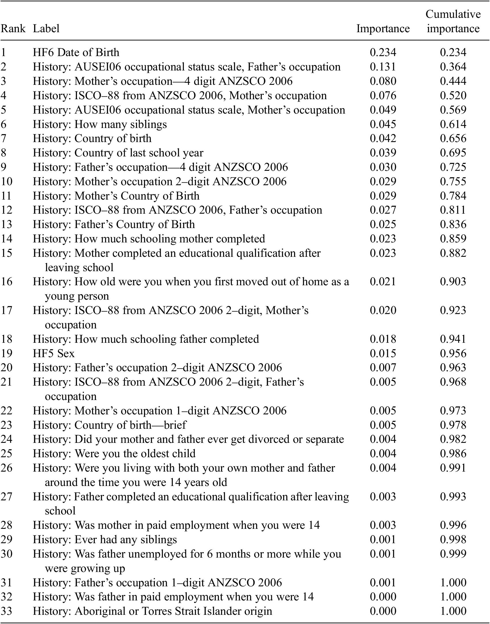
These variables were chosen out of almost 6993 possible controls in the dataset because when trying to orthogonalize we can only use pre-treatment variables (Chernozhukov et al., Reference Chernozhukov, Chetverikov, Demirer, Duflo, Hansen, Newey and Robins2018; Hünermund et al., Reference Hünermund, Kaminski and Schmitt2021) and most of the variables could be considered post-treatment because present income is being measured in most cases years after the respondent was last in education.Footnote 4
Finally, it may be useful to include certain post-treatment variables in the heterogeneity model but not in the nuisance models (e.g., the number of children someone has had). These cannot be controls because they are post-treatment but could be important moderators (Pearl, Reference Pearl2009). For example, women who have children after their education tend to have lower incomes than similar women who did not have children and therefore lower returns on education (Cukrowska-Torzewska and Matysiak, Reference Cukrowska-Torzewska and Matysiak2020). These would be bad controls in the nuisance models (Hünermund et al., Reference Hünermund, Kaminski and Schmitt2021), but improve fit and help us to uncover the presence of an important motherhood effect in the heterogeneity model (Celli, Reference Celli2022; Watson et al., Reference Watson, Cai, An, Mclean and Song2023). However, while grf can handle different sets of variables for different models, this is not the case for the EconML package in Python which we use to generate SHAP value plots. For this reason, we choose a more limited model (and suggest EconML change its approach to be more like that of grf).
The causal forest produces an ATE estimate of $20,455 for a bachelors degree with a standard error of $2001. The real value of the method though is of course in analyzing CATEs which we will do through XAI and IAI lenses. While neither of these groups of tools actually amount to showing a causal relationship that variables might in driving treatment effect variation, these results are still useful in seeking to understand causal effects.
6. Transparency in the Queensland case study
6.1. Using XAI tools
This section considers how the transparency problems might be addressed and what issues may be insurmountable. For the most part, the issues of understanding and oversight will be combined as they both encounter similar technical barriers. There are two main XAI approaches that have been proposed for the causal forest, the first is a more classic predictive machine learning approach in SHAP values (Lundberg and Lee, Reference Lundberg and Lee2017). The second is a variable importance measure which has somewhat more humble ambitions—it does not seek to quantify the impact of each variable in each case but instead tries to show which variables are most important in fitting the forest.
6.1.1. SHAP
We start by using an XAI approach, in particular the SHAP method which has previously been applied to causal forest analysis (Tiffin, Reference Tiffin2019). SHAP values decompose predictions into an additive combination of effects from each variable for a local explanation (i.e., the contribution of each variable is only locally to that part of the covariate space) (Lundberg and Lee, Reference Lundberg and Lee2017). SHAP values are based on Shapley values which provide a fair way to portion out a pay-off amongst a number of cooperating players in game theory. It does this by considering how the prediction changes when different sets of features are removed (set to a baseline value) versus when they are included (Lundberg and Lee, Reference Lundberg and Lee2017). More details on the calculation of SHAP values can be found in Lundberg and Lee (Reference Lundberg and Lee2017). In this case, the pay-off is the difference between the causal forest prediction and the average treatment effect and the players are the different covariates. It uses the predictions of a causal forest in much the same way it would use the predictions of a predictive random forest to generate SHAP explanations.
Unfortunately, good methods to calculate SHAP values exist only for forests implemented in the Python EconML package, not the R grf package. Conversely, the EconML package lacks some of the features of grf and is implemented slightly differently. This accounts for differences in results between these outputs and the grf outputs in other sections. In addition, due to the long time to compute SHAP for a large ensemble, we use an ensemble of just 1000 trees here.
It is worth stating that it is not clear that SHAP values are suitable for this application. There is some question among the maintainers of grf as to whether SHAP values are appropriate for a causal forest given the way the forest is used to construct kernel weights rather than directly estimating based on aggregated predictions (grf-labs, 2021). This argument would apply in theory to any predictive XAI tool which does not account for the specific estimation strategy of the generalized random forest estimators (Athey et al., Reference Athey, Tibshirani and Wager2019).
There are two different ways to visualize SHAP, as an aggregate model showing all the SHAP effects for the sample as in Figure 1 or in a waterfall plot which breaks down the specific local effects for a single observation as in Figure 2. The aggregate plot graphs effect as x coordinate and variable value as color. It ranks the variables in terms of the magnitude of SHAP effects. In a waterfall plot, feature names and values for a specific case are shown on the right and the effect that feature has on the CATE is shown as a red (positive) or blue (negative) bar. This deviation is from the average treatment effect. On the aggregate summary plot, the value on CATE estimate is shown on the x-axis and the feature value leading to that estimate is shown on the color scale (per the bar on the right of the plot).
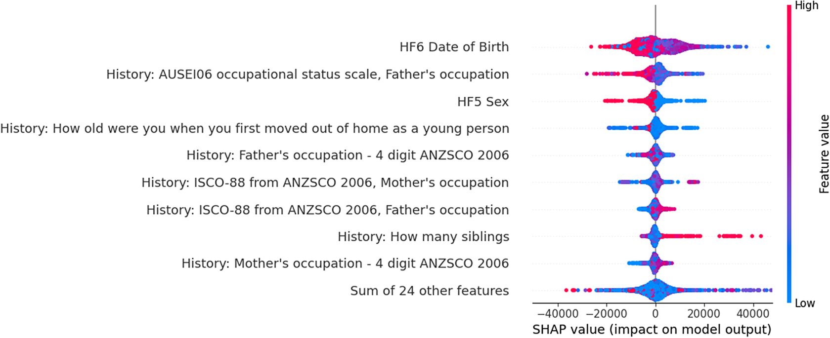
Figure 1. Aggregated SHAP plot explaining the HTE estimate across the distribution.

Figure 2. Individual-level waterfall plots.
Interpreting the aggregate plot, we can see that age is the most important predictor. Generally, younger people (those with a higher date of birth value) benefit less from a degree than older people. Having a father with higher occupational status seems to also decrease the benefits, perhaps due to higher social mobility benefits for having a degree amongst people from lower class backgrounds. Men (1 on sex) benefit more than women (2 on sex) from a degree.
While there are other patterns here, the plot is somewhat overwhelming, it can be hard to unpick patterns here outside of very high-level ones. Looking at waterfall plots can help offer a more nuanced picture. Here we present three waterfall plots, though the precise variable values have been blurred to avoid reporting raw values for HILDA participants (HILDA data access is subject to an approval process). However, even without this values, this should give a sense of the utility of these plots.
While SHAP values might be useful they are by their nature local explanations and so it can be hard to extract insight from them for either usability or accountability.
SHAP values—assuming their validity with the causal forest—can be an excellent aid for usability. SHAP values give arguably a more “causal” insight than simply graphing distributions across variables,Footnote 5 as it aims to take account of the additional effect of a given variable where our plots of effect distributions simply give a visual sense of correlation. This can help to understand patterns in causal effects that may have been missed otherwise. SHAP plots can even give a sense of interactions between features when viewing a number of different waterfall plots. For example, if having children hurts women’s incomes, particularly the decade after the birth of a child, we might see age have a different treatment effect for women than men. While there might be good information here, this is also a drawback. There is also a lot of information that needs to be processed to help a human decision-maker understand causal effects and make a decision and as all these explanations are local. The user may be simply missing the important patterns and not know it because they are awash in useless data. This is not to mention the information from the nuisance models that could be gained through SHAP analysis as well.
SHAP is intuitively useful for accountability because it lays out variable effects in an easy-to-understand way and can be used to break down effects at the individual level. However, this convenience is somewhat misleading. The problem is that SHAP is a relatively poor approach to accountability because it cannot explain the human element in a joint decision-making process. The amount of data it provides on the underlying models can be simply overwhelming, but it also obscures the core question, how did a human make a decision that had real-world consequences based on this model? What local effects were generalized into evidence? What evidence was interpreted as showing underlying causation? What local effects were ignored?
One benefit of SHAP for both usability and transparency though is that it is well-suited to the diagnosis of problems in the model, for example, biasing “bad controls” would show up among the most impactful variables. Equally, variables that should have a large effect but which are not present among the top variables may suggest errors in data. Finally, the local level explanations which we have previously suggested is a limitation could be useful to individuals trying to find modeling errors for accountability as for example, it could allow an individual to examine SHAP scores in their own case and see if the results match their priors about causal effects in their own case. Exactly how to go about updating modeling approach versus ones priors is a tricky question that is beyond the scope of this article but would be an interesting avenue for future research. It is worth noting as a final point that SHAP values may be infeasible for larger models and larger datasets. SHAP is relatively time-complex and so trying to explain results may prove computationally infeasible for large models (Bénard and Josse, Reference Bénard and Josse2023).
6.1.2. Variable importance in heterogeneous treatment effect estimation
Variable importance seeks to quantify how impactful each variable is in a given model. In predictive modeling where the techniques were invented, there are several methods for doing this aided by access to ground-truth outcomes. For example, we can sum the decrease in impurity across all splits for a given variable or see how performance suffers by randomly permuting a given feature (Saarela and Jauhiainen, Reference Saarela and Jauhiainen2021). In the causal forest context (at least in the grf package), we lack ground truth and so have to use more heuristic or computationally complex approaches.
There are two main approaches to variable importance. The first—which is the simpler of the two—is about counting uses of the variable in a causal forest. It was developed for the grf package. In this approach, variable importance is measured with a heuristic where the value is a normalized sum of the number of times a variable was split on weighted by the depth at which is appeared (by default, exponential halving by layer) and stopping after a certain number (by default four) to improve performance (Athey et al., Reference Athey, Tibshirani and Wager2019). This is a relatively naive measure (something the package documentation itself admits), the naivete is made necessary by a lack of ground truth which prevents the package from using the more sophisticated approaches that predictive forests tend to rely on (Louppe et al., Reference Louppe, Wehenkel, Sutera, Geurts, Burges, Bottou, Welling, Ghahramani and Weinberger2013). This means a whole rethink of the approach to generating variable importance measures is needed, but finding a more sophisticated approach was outside the scope of the grf package which was focused on just laying the groundwork for the generalized random forest approach (Athey et al., Reference Athey, Tibshirani and Wager2019).
Taking this depth-weighted split count approach, the variable importance for the forest is shown in Table 1. We see interestingly that the top 10 variables cumulatively making up 76% of depth-weighted splits. Variable importance clearly gives less information about predictions than the SHAP plots (assuming the validity of applying SHAP to the causal forest), however, it does tell us some similar things about the factors that seem to drive heterogeneity in causal effects. It is also an approach that is less controversial than the use of SHAP.
A more sophisticated version of variable importance is implemented in the mcf package (Lechner, Reference Lechner2019) which uses permutation variable importance to estimate variable importance metrics. It does this by randomly shuffling values for each variable in turn and then predicting out new estimates. The change in the error for those predictions gives a sense of how important a given variable is in the model structure. Another approach is taken in recent work by Hines et al. (Reference Hines, Diaz-Ordaz and Vansteelandt2022) and Bénard and Josse (Reference Bénard and Josse2023) which tries to estimate the proportion of total treatment effect variance explained by each variable used to fit the causal forest. These two recent approaches both work by retraining many versions of a causal forest with and without variables and finding what percentage of treatment effect variation is explained when a variable is added in. This can be very computationally complex in ensembles of the size being used in this article and so we do not estimate these variable importances.
Variable importance has humbler ambitions than SHAP and arguably benefits from this when it comes to being of use for transparency. Variable importance provides much less data which in turn means it is less likely to be misinterpreted and less likely to be relied on to actually understand the model rather than be a jumping-off point for exploratory analysis. It also provides an arguably more global explanation by simply summarizing the structure of the causal forest rather than trying to explain individual estimates.
The question is though, does this more limited ambition help in achieving usability or accountability? On usability, variable importance can be a good tool for exploratory analysis for example in identifying possible drivers of heterogeneity for which heterogeneity can be explored further (e.g., by graphing the effect or by modeling doubly robust scores with a parametric model). In addition, it can be useful for sense-checking that all variables involved are “good controls.” Any variable that is going to have a substantial biasing effect ala collider bias will have to be split on in order to have a biasing effect. It should therefore show up in the variable importance calculation. There is obviously more that needs to be done to explain heterogeneity than just counting splits. Variable importance is—at its best—the starting point for further analysis of usability.
On accountability, variable importance is not particularly useful because it is such a high-level summary of the model being used. If there are for example unjust outcomes occurring because of the model, it is hard to tell this simply from variable importance. By an unjust outcome we mean that somewhere in the complexity of estimating effects, poor local centering, poor estimation of CATEs, poor communication of CATEs, the model has given decision-makers a false impression about the underlying causal relationships this leads them to make an “unjust” decisions. While we are happy to defer to the role of decision-makers to decide their own definition of justice, modeling which does not allow the decision-maker to make decisions to better their own definition of this is unjust. This is admittedly a convoluted definition but one which is necessary given the indirect relationship between model predictions and decisions compared to the more direct relationship in predictive modeling (Rehill and Biddle, Reference Rehill and Biddle2023). For example, in predictive contexts, it can be useful to see if a sensitive variable (or its correlates) has any effect on predicted outcomes with a model being fair if outcomes are in some way orthogonal to these sensitive variables (Mehrabi et al., Reference Mehrabi, Morstatter, Saxena, Lerman and Galstyan2019). In the causal context on the other hand it can be important to know that marginalized groups have lower predicted treatment effects for example because a linguistic minority cannot access a service in their own language. In fact, it would be unjust if modeling failed to reveal this and so a decision-maker not understanding this treatment effect heterogeneity could not act to improve access to the program. Just seeing splitting on certain variables then is not indicative of a particularly unjust model—yet this is the only level of insight we get from variable importance.
6.2. Using IAI tools
We can see that when using XAI tools there is a large amount of information to process, and we cannot get a global understanding of how the model works. We might then want to turn to interpretable models. There are two main ways of doing this. The classic approach to IAI for a random forest is to simplify the ensemble down to a single tree as this does not involve additional assumptions (Sagi and Rokach, Reference Sagi and Rokach2020). In the case of the causal forest, another approach that is often taken is to simplify the forest down to a best linear projection of heterogeneity (Athey and Wager, Reference Athey and Wager2019). This imposes additional assumptions but provides a model that is interpretable to quantitative researchers and in particular, allows for hypothesis testing.Footnote 6
6.2.1. Extracting a single tree
While there are lots of individual trees in the causal forest and one could pick one (or several) at random to get a sense of how the forest is operating, there are also more sophisticated approaches that provide ideally a tree that is better than one just chosen at random. Wager (Reference Wager2018) suggests a good way to find a representative tree would be to see which individual tree minimizes the R-Loss function of the causal forest. This is not a peer-reviewed approach, nor one which has even been written up as a full paper but it represents the best proposal specific to the causal forest that we have. Other approaches attempt to distill the knowledge of the black box forest into a single tree that performs better than any individual member of the ensemble (e.g., in Domingos, Reference Domingos1997; Liu et al., Reference Liu, Dissanayake, Patel, Dang, Mlsna, Chen and Wilkins2014; Sagi and Rokach, Reference Sagi and Rokach2020). However, the problem here is that even the smartest methods for extracting a tree of sufficient simplicity to be interpretable require problems where there is enough redundancy in rules—the underlying structure can be captured almost as well by a few splits in a single tree as by many splits in a large ensemble—that the problem can be simplified to the few best rules with relatively little loss in performance. Rather than focusing on methods for extracting the best tree then, we instead look at whether enough redundancy exists in this problem to make simplification to a reasonably good tree feasible, analysis that to the best of our knowledge has not been done for an application of the causal forest.
The exact marginal trade-off of adopting a more interpretable model depends on what Semenova et al. (Reference Semenova, Rudin and Parr2022) call its Rashomon Curve. The Rashomon Curve graphs the change in performance as a model is simplified in some way, for example by a reduction in the number of trees in a random forest until it becomes a single tree. In Figure 3, we show a Rashomon curve comparing the performance of a causal forest (i.e., the final heterogeneity model) of 50,000 trees against one of 1, 10, 100, 1000, and 10,000 trees and a tree distilled from the 50,000 tree forest.
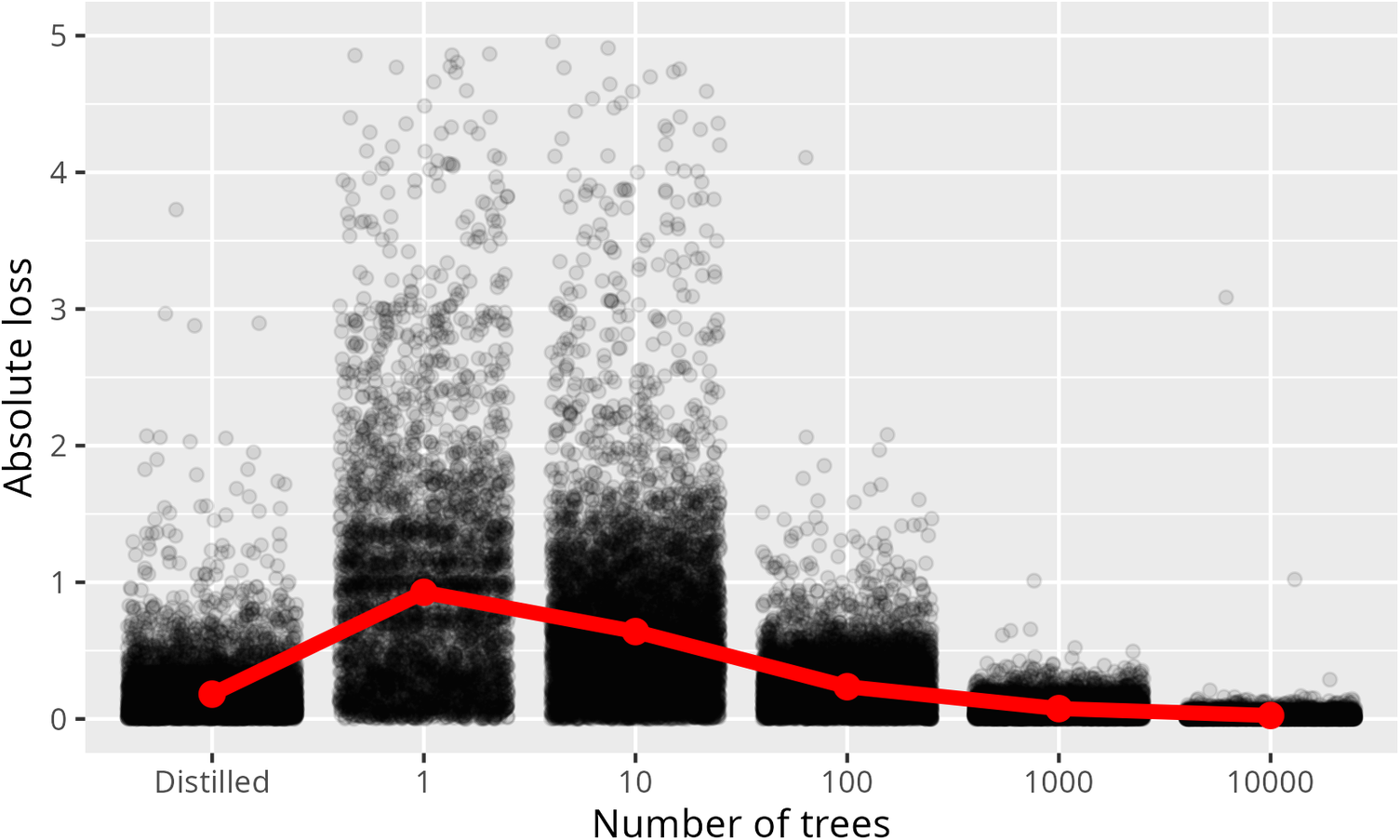
Figure 3. Rashomon curve for the effect of heterogeneity estimating model size showing absolute loss as a proportion of the original estimates for a variety of model sizes. Note: The y-axis is cut off at 5 for clarity. A small portion of points are above this line though these are still incorporated into the mean.
In these figures, error between the large model (
 $ {\hat{\tau}}_L $
) and the smaller models (
$ {\hat{\tau}}_L $
) and the smaller models (
 $ {\hat{\tau}}_S $
) is
$ {\hat{\tau}}_S $
) is
 $ \left|\frac{{\hat{\tau}}_L-{\hat{\tau}}_S}{{\hat{\tau}}_L}\right| $
. Because we lack ground truth and know that accuracy should increase as number of trees increases, performance relative to a large forest should give a good indication of performance relative to ground truth. In all cases, these used identical nuisance functions each fit on 10,000 trees. This reveals substantial loss in accuracy as the size of the forest shrinks, this accuracy is due to an increase in what the grf package calls excess error—error that would shrink toward zero as ensemble size approaches infinity (as opposed to debiased error which is not a function of forest size). The Rashomon curve here may be flatter for problems with lower excess error, however, in this case, the trade-off for moving to a single tree seems to be a poor one. To put it in concrete terms, the mean absolute loss for moving from 50,000 trees to a single tree was 107% of the comparison value on average.
$ \left|\frac{{\hat{\tau}}_L-{\hat{\tau}}_S}{{\hat{\tau}}_L}\right| $
. Because we lack ground truth and know that accuracy should increase as number of trees increases, performance relative to a large forest should give a good indication of performance relative to ground truth. In all cases, these used identical nuisance functions each fit on 10,000 trees. This reveals substantial loss in accuracy as the size of the forest shrinks, this accuracy is due to an increase in what the grf package calls excess error—error that would shrink toward zero as ensemble size approaches infinity (as opposed to debiased error which is not a function of forest size). The Rashomon curve here may be flatter for problems with lower excess error, however, in this case, the trade-off for moving to a single tree seems to be a poor one. To put it in concrete terms, the mean absolute loss for moving from 50,000 trees to a single tree was 107% of the comparison value on average.
An alternative approach is to use distillation to improve performance. Distillation of black-box models to a single tree can improve the performance of a tree over simply fitting that tree on the same data the black-box learner or “teacher” was fit on. Exactly why this is the case is not yet entirely clear but it is a useful empirical technique (Hinton and Frosst, Reference Hinton and Frosst2017; Dao et al., Reference Dao, Kamath, Syrgkanis and Mackey2021). Importantly, many of the characteristics useful for causal inference, also make the forest a good candidate for being a distillation teacher as Dao et al. (Reference Dao, Kamath, Syrgkanis and Mackey2021) argue distillation is a semiparametric inference problem much like machine learning of causal quantities. They adjust the teacher using cross-fitting and loss correction inspired by double machine learning. The use of distillation with causal forests has recently been proposed by Rehill and Biddle (Reference Rehill and Biddle2024). Here we compare the performance of the basic single tree model against a distilled model. We show that the performance of the distilled model is much better than the single tree trained on the raw data and is somewhere between the 100 and 1000 tree ensembles trained on raw data in its performance predicting the 50,000 tree ensemble predictions.
Reducing a model to a single tree would be very useful for both usability and accountability. In both cases, the entirety of the model can be comprehended by people using that model to make decisions and people critiquing the model. The problem is that the trade-off may simply not be worth it. There are already very interpretable methods for quantitative research that are well understood. This is not to mention that there is a much larger suite of methods drawing on the latter approach for removing selection bias that does not involve trying to model out confounding with a relatively simple model (like a linear model or decision tree). For example, a practitioner could use instrumental variable regression, difference-in-differences etcetera. So even though it may be possible to fit an interpretable model to proxy the causal forest, there will likely be a performance cost to the simplicity (Rudin, Reference Rudin2019). At least in the case of this application, there is a stark trade-off between interpretability and performance for simply reducing the number of trees. However, distillation allows for a single, interpretable tree with the performance of a moderately sized ensemble in this case.
6.2.2. Using a best linear projection
One approach to fitting an interpretable model that draws on the power of the causal forest is to fit a best linear predictor (BLP). The BLP is a relatively well discussed approach compared to others discussed in this article. It was an approach proposed by Semenova and Chernozhukov (Reference Semenova and Chernozhukov2021), incorporated into the grf package and applied by Athey and Wager (Reference Athey and Wager2019) in the most widely cited application of the causal forest. Undoubtedly the BLP adds value, particularly for hypothesis testing of results. However, its utility is situational. It assumes that a linear projection of the CATE onto a set of covariates (which may or may not be the predictors used in the causal forest) is useful in some way. This may mean that it meets the assumptions necessary for linear regression with valid standard errors, however, it may be useful in a less formal way, for example in indicating potential drivers of heterogeneity which can then be explored in other ways. It also has the potential however to be misleading if used as the only way to try and understand treatment effect variation (it is easy to imagine for example very heterogeneous nonlinear distributions of CATEs that might produce a linear model with slope coefficients close to zero). It goes without saying that projecting effects with high-dimensional interactions between variables onto a combination of these variables will miss these important interaction effects.
Because its utility depends on the situation, BLP should work well as a tool for usability of the causal forest when used responsibly (i.e., when assumptions hold). The BLP was invented for this kind of application and allows researchers (or policy analysts) more familiar with linear models to make sense of the complex causal forest. However, they offer less value as accountability tools. The reason for this is that taken alone they provide little insight into the workings of a model that may lead to unjust outcomes (unless policy was made solely on the basis of the BLP).
Table 2 shows the regression output for the BLP of returns on education in Australia. In this case, it projects doubly robust scores onto some of the most important variables in the causal forest. The BLP needs to be considered with more care than the causal forest as we are now actually hypothesis-testing results and making a functional form assumption. This means it makes sense to exercise some judgment about variable choice. For example, variables with very similar underlying constructs do not all belong here unless there is a good reason to control for or separately estimate their effects. In this analysis we pick variables measuring the construct of age (date of birth in UNIX time that is where 0 is the first of January 1970), parents’ occupations (occupational status measured on the AUSEI06 scale for both mother and father which measures status on a 0–100 scale), number of siblings and country of birth encoded as a dummy (with Australia as the base case and countries with fewer than 100 respondents excluded to keep the table brief).
Table 2. Best linear projection of doubly robust scores onto selected covariates
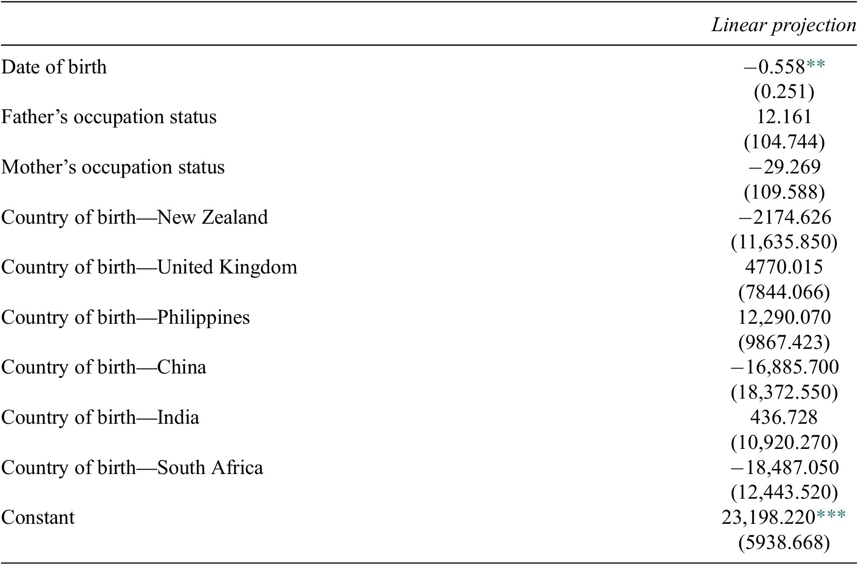
Note. Base case for country of birth is Australia.
** p < 0.05;
*** p < 0.01.
In this analysis, only one variable shows a statistically significant effect on treatment effect heterogeneity, that is date of birth with younger people (people with higher date values) having lower earnings effects from education. There are many possible reasons for this. This may be because older people may have had more time to recognize the benefits of education or because education levels as a whole have gone up meaning younger people going into a given profession have a higher level of education than older people who are already established there.
It is also worth noting a BLP can be fit directly on doubly robust scores without a causal forest involved (although fitting a BLP through the grf package is helpful as jackknifing errors with the structure of the ensemble is a computationally cheap way to estimate standard errors where otherwise nuisance models would need bootstrapping).
6.3. Identifying problems in nuisance models
While this section has for the most part focused on transparency in the heterogeneity model, it is worth discussing briefly transparency in the nuisance models. The transparency needs in nuisance models are different from those in heterogeneity models. There is no need to understand the nuisance models from a usability point of view. We just need to be able to diagnose problems in identification that might come from poor-performing nuisance models, it does not actually matter how these models work. In accountability concerns, the important thing is that we correctly identify effects, there is no equity concern outside of models performing identification poorly in ways that might harm people for whom identification is poor (Rehill and Biddle, Reference Rehill and Biddle2023). However, this is not a case of fair outcomes being counter to the goal of modelers, rather good identification is something that all parties want and which can be achieved through a simpler set of tools. Here we look at refutation tests and checking propensity score balance as two possible diagnostics.
6.3.1. Refutation tests
Refutation tests could be considered a kind of narrow causal AI algorithmic transparency tool. These are diagnostic tools developed for generic causal modeling approaches (Sharma et al., Reference Sharma, Syrgkanis, Zhang and Kıcıman2021). While they do not give much insight into the underlying causal effects, they are very useful to diagnosing problems in modeling either for users who want to make sure their models meet their assumptions or for those who wish to critique models. They are tests of the underlying causal assumptions of a model, however, they can also diagnose problems with the nuisance modeling approaches insofar as nuisance models may be failing to properly model out confounding effects. In this way, they refute analysis but do not necessarily provide a good idea of how one might fix the problem of confounding.
We test two particular refutation approaches by randomly shuffling treatment and then outcomes. This functions as a version of the placebo treatment and dummy outcome test that preserves the underlying univariate distribution while rendering it independent from other variables (Sharma et al., Reference Sharma, Syrgkanis, Zhang and Kıcıman2021). These estimates are made with 10,000 tree causal forests and are plotted against the real treatment or outcome models to check if poor nuisance model fit is affecting treatment effect estimates. We then look at whether treatment effect estimates move to zero. Random treatment should in a correctly specified model drive the ATE and CATE estimates to zero (Sharma et al., Reference Sharma, Syrgkanis, Zhang and Kıcıman2021). Table 3 records the average treatment effect models for these tests. In neither case is there a statistically significant average treatment effect after randomization.
Table 3. Average-level results of refutation tests

To examine these results in more detail, Figure 4 shows results across the treatment and outcome distributions. The refutation tests seem to work well for placebo treatment, but when randomizing income, predicted treatment effect is not orthogonal to actual treatment. This may suggest a problem with identification that should be investigated further, for example by considering finding more data for use in the nuisance models or by investigating other identification approaches. Importantly though, as the actual causal estimates are doubly robust and the placebo model is working well, problems in the outcome nuisance model may not be biasing the treatment effect estimates.

Figure 4. Effect of refutation tests on estimated treatment effects (treatment effects should be near zero, conditional averages are averages of doubly robust scores, not the individual estimates shown as points).
This kind of analysis is mostly useful for usability. The reason for this is that running placebo tests would ideally be part of diagnosing a model’s problems before it is used (Sharma et al., Reference Sharma, Syrgkanis, Zhang and Kıcıman2021). While identification problems could pose justice issues that might be of interest for accountability, the problem is that confounding is not really a problem of the individual or small-group kind of accountability involves. To the extent there are confounding issues not identified by analysts at the time the model is fit, it is hard to understand whether the causal effect is estimated better or worse for certain individuals across all the possible covariates. It is equally hard to comment on the extent to which such confounding effected an unjust outcome.
6.3.2. Propensity score balance
As with any design relying on propensity scores, it can be useful to check for problems in identifying assumptions by graphing the overlap in propensity scores. These checks have been published in a minority of papers using the causal forest but running (or at least publishing) the results of these tests is not yet established best practice (Rehill, Reference Rehill2024).
The implications of this test for bias in estimates are less clear than in a pure inverse probability weighting design as there is also the effect of the outcome nuisance model to consider. However, poor overlap is certainly not a good sign and may affect the credibility of the design. Figure 5 shows the propensity score densities in the returns on education study. There is reasonable overlap between the distributions but there is also a large portion of scores at the low end of the range where there is no overlap. This is a problem and it may be worth using propensity score trimming—at least as a robustness check.
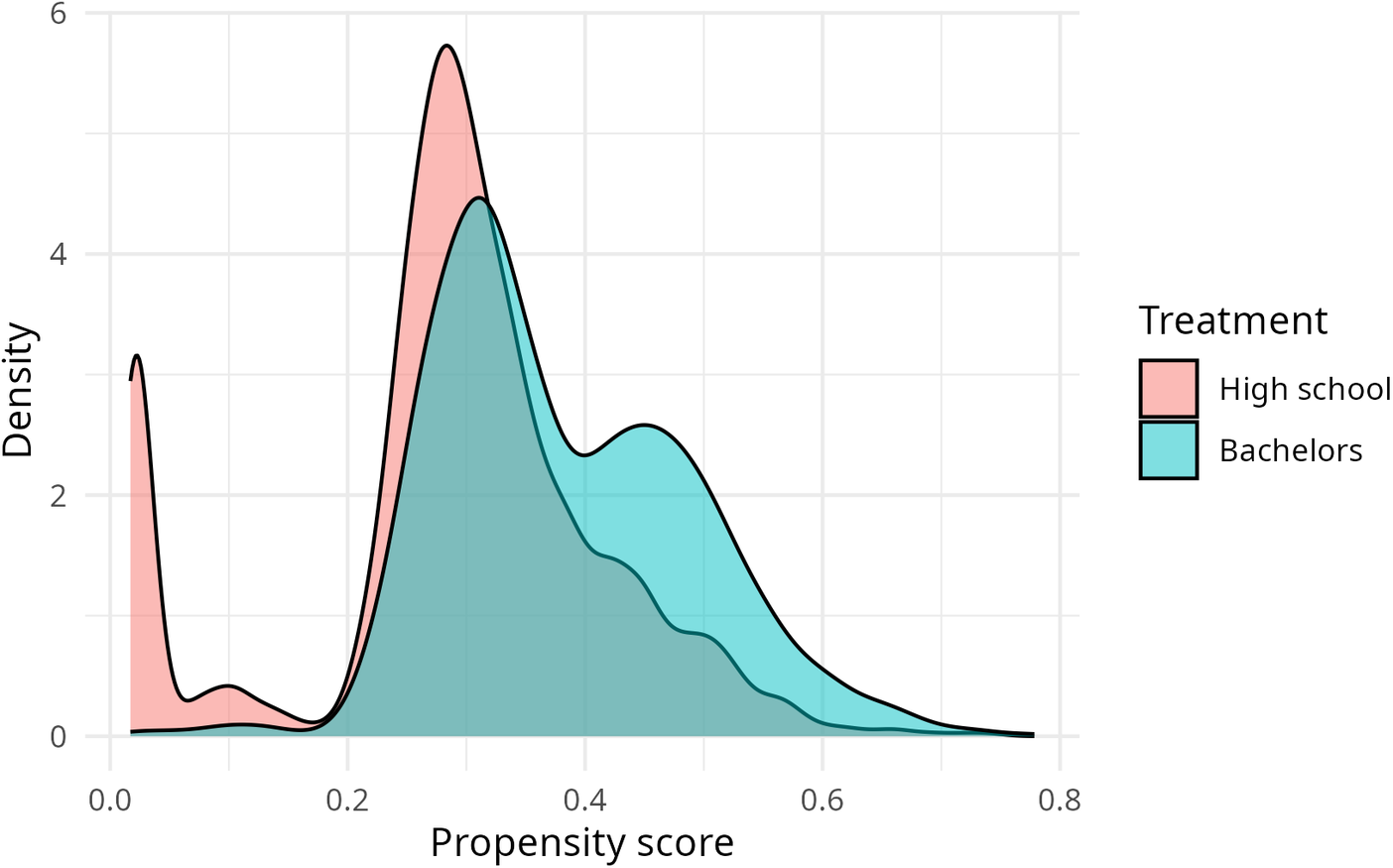
Figure 5. Propensity score densities.
7. Conclusion
Causal machine learning offers tremendous promise to researchers tackling specific kinds of research questions, but transparency poses a real problem both to users of the model and those who might want to hold these users accountable. This article has laid out some issues around the use of causal machine learning in policy research around government decisions, but it is far from a full survey of all the possible issues that might arise. A much larger body of knowledge is needed to properly establish best practice for the use of these methods. In particular studies on the use of causal machine learning methods applied to real-world policy problems as these case studies become available would be useful, as would experiments on how causal machine learning analysis affects decision-making when compared to traditional quantitative methods along the lines of Green and Chen (Reference Green and Chen2019) or Logg et al. (Reference Logg, Minson and Moore2019) on predictive systems.
In the absence of a significant existing critical literature, we offer the following two guidelines for using causal machine learning. Firstly, causal machine learning should only be used where it is additive to the evaluation. By that we mean there is a reason to use a powerful but black-box method over a less powerful but interpretable method (i.e., standard policy evaluation methods). The obvious reason to do this in the case of the causal forest is when it will be valuable to understand heterogeneous effects at the individual level or where we have little theoretical knowledge about the drivers of heterogeneity and so have to undertake a data-driven exploration of these effects instead (Athey and Imbens, Reference Athey and Imbens2018). Causal machine learning methods should not be used for high-stakes policy evaluation simply because they are novel or because it is inconvenient to find quasi-experimental/experimental data. The decision to use them should be made understanding that there will likely be responsibility gaps in the use of such novel methods in policy-making (Matthias, Reference Matthias2004; Olsen, Reference Olsen2017). Secondly, causal machine learning should meet the standards of transparency expected from predictive machine learning or traditional causal modeling in government. Just because the nature of the analysis is different does not mean the same issues that currently plague machine learning models used in government are not a concern for causal models.
Within this article, we have tried to establish why transparency is important in causal modeling, analogizing this to predictive applications. However, we have also laid out how predictive and causal analysis bring with them different transparency needs. Causal machine learning lays out the data-generating process of the underlying data and the fits into a process of human decision-making with well-established transparency requirements. On the other hand, these machine learning models usually involve fitting several black-box models where even XAI and IAI approaches fail to explain much about how all these models relate to each other (there are not even good procedures for estimating error through the process). While this article has provided some examples of approaches that can help make causal machine learning more usable and accountable, there are still many questions from the theoretical (how do we weigh possible accountability gaps against more powerful modeling?) to the very practical (is it valid to apply SHAP to causal forest predictions?) that remain open. As these methods begin to be used more and more, it is important that a critical literature which can highlight and solve transparency problems grows alongside them.
Data availability statement
The data used for the case study in this article are available from the Australian Data Archive at https://www.doi.org/10.26193/KXNEBO. They require an application to access. The code used is available at https://github.com/pbrehill/Transparency-CausalForest.
Acknowledgments
P.R. is supported by an Australian Government Research Training Program Scholarship.
Author contributions
Conceptualization: P.R.; Investigation: P.R.; Methodology: P.R.; Supervision: N.B.; Validation: P.R.; Visualization: P.R.; Writing—original draft: P.R.; Writing—review and editing: P.R., N.B.
Funding statement
This work received no specific grant from any funding agency, commercial, or not-for-profit sectors.
Competing interest
The authors declare no competing interests in relation to this work.
A. Appendix: Table of definitions
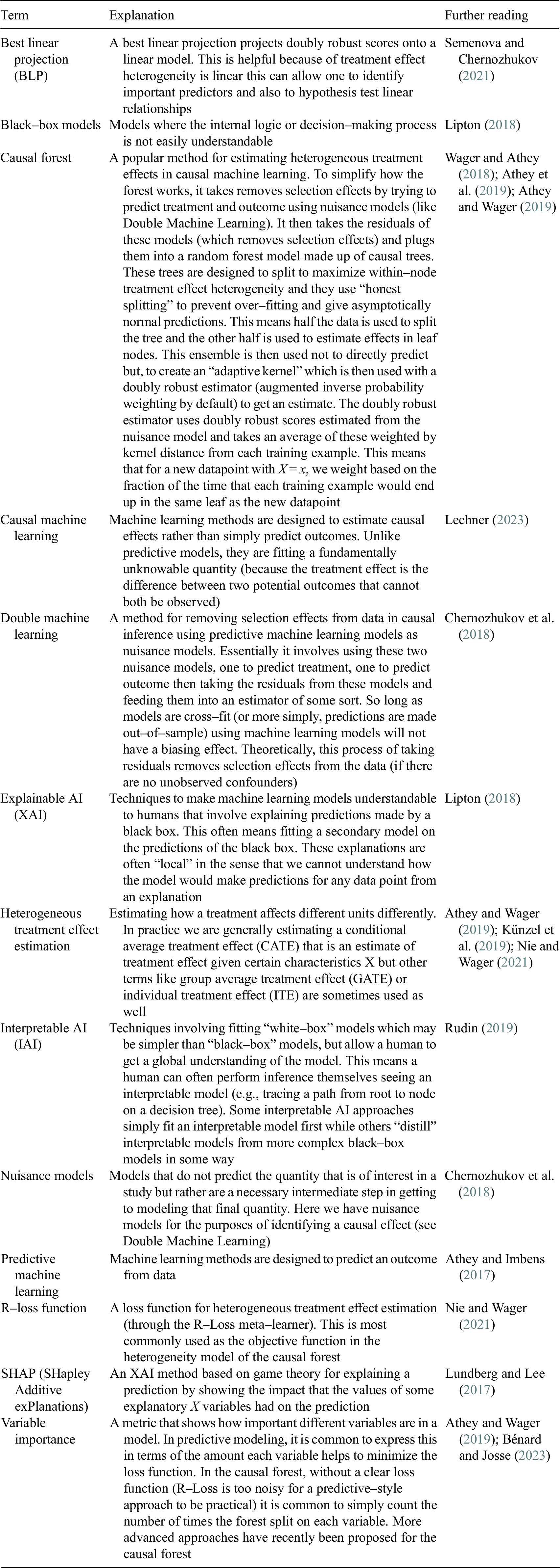


 Open access
Comments
No Comments have been published for this article.