


1. Introduction
The growing demand for high-performance fiber reinforcements in various industries has increased the need for automated weaving equipment, such as in aerospace, shipbuilding, and automotive [Reference Bilisik1, Reference Li, Shan, Du, Zhan, Li and Liu2]. As a result, robots are gradually being integrated into preform weaving, replacing manual operations of yarn storage. This shift toward automation not only significantly improves efficiency but also reduces labor costs and ensures product consistency [Reference Xu, Meng, Li and Sun3]. However, path planning is crucial to fully utilize robot technology. Selecting an appropriate path planning method based on the object being processed and the application scenarios is key to enhancing production quality and efficiency.
The robot must move from its starting point to the ending point without encountering any obstacles to ensure safe path planning. To achieve this, researchers have developed various algorithms suited for different environments, which can be categorized into four types based on their implementation principles. The first type includes graph search methods like the Dijkstra algorithm [Reference Fadzli, Abdulkadir, Makhtar and Jamal4, Reference Mirahadi and McCabe5], A* algorithm [Reference Warren6], and D* algorithm [Reference Ferguson and Stentz7]. The second type is local planning methods like the artificial potential field method [Reference Chen, Wu and Lu8, Reference Wang, Zhu, Wang, He, He and Xu9] and eplastic bands [Reference Quinlan and Khatib10]. The fourth type refers to intelligent optimization methods, which include particle swarm optimization algorithm [Reference Huang, Zhou, Ran, Wang, Chen and Deng11, Reference Lin, Liu, Wang and Kong12], ant colony algorithm [Reference Luo, Wang, Zheng and He13], genetic algorithm [Reference Lamini, Benhlima and Elbekri14], and reinforcement learning [Reference Chehelgami, Ashtari, Basiri, Masouleh and Kalhor15]. Finally, the forth type consists of random sampling methods, such as the probabilistic roadmaps (PRM) algorithm [Reference Bohlin and Kavraki16, Reference Sánchez and Latombe17] and the rapidly expanding random trees (RRT) algorithm [Reference Wang, Zhang, Fang and Li18–Reference Xinyu, Xiaojuan, Yong, Jiadong and Rui20]. The first three types of methods can be widely applied to mobile robots in two-dimensional planes, but they are difficult to be applied to path planning in the joint space for robots with high degrees of freedom. The basic RRT algorithm and its variants, such as RRT* [Reference Noreen, Khan and Habib21] and Bi-RRT [Reference Ma, Duan, Li, Xie and Zhu22], are tree structure algorithms based on random sampling, which are widely used in motion planning for multidegree-of-freedom robots. However, the RRT algorithm has drawbacks such as strong randomness, long planning time, and poor path smoothness. Researchers have made improvements to the RRT algorithm to enhance its rapid expansion capability. One of these enhancements involved modifying the extension direction by adding the vector sum of random gravity and target gravity [Reference Cao, Zou, Jia, Chen and Zeng23]. This alteration increased the probability of reaching the target point, leading to faster convergence and reduced computational time. Nevertheless, using a fixed gravity coefficient would lead to a higher planning failure rate when dealing with complex obstacles. Some works focused on improving the step size by introducing an adaptive step size RRT algorithm [Reference An, Kim and Park24], which calculated the maximum allowable step size for each iteration in the joint space under the constraint that the maximum distance of each link’s movement is always less than the minimum obstacle width, thereby improving the accuracy of obstacle avoidance. Based on this, this paper introduces an Improved rapidly expanding random trees (IRRT) approach with adaptive direction and step size to enhance the planning performance of robots in challenging weaving environments with complex obstacles.
With the rise of complex application environments for robots, tasks like polishing [Reference Zhu, Feng, Xu, Yang, Li, Yan and Dang25], welding [Reference Shahabi, Ghariblu, Beschi and Pedrocchi26], and playing table tennis [Reference Mülling, Kober, Kroemer and Peters27] have become more difficult, requiring improved path planning. To address this, researchers have explored learning from demonstration (LfD) methods that can learn task actions and skill features from manual demonstrations. One such method is the dynamic motion primitives (DMP) based on nonlinear dynamic systems [Reference Ijspeert, Nakanishi and Schaal28, Reference Davchev, Luck, Burke, Meier, Schaal and Ramamoorthy29]. However, DMP requires precise models and struggles to account for uncertainty in teaching results. To account for uncertainties in teaching results, researchers have put forth the Gaussian mixture model (GMM) method [Reference Calinon, Guenter and Billard30, Reference Rozo, Jiménez and Torras31]. However, this approach requires extensive teaching data. As a result, researchers have developed and enhanced these methods. In literature [Reference Yang, Chen, He, Cui and Li32], a motion model was created using DMP, and GMM was utilized to estimate the nonlinear function of the motion model, allowing for the extraction of more skill features in robot motion. In addition, the neural network is a common method for LfD, which includes the multilayer neural network method [Reference Liu and Asada33], radial basis function neural network [Reference Kaiser and Dillmann34], and extreme learning machines (ELM) [Reference Duan, Ou, Hu, Wang, Jin and Xu35]. Among them, the ELM, a single hidden layer neural network algorithm [Reference Ding, Zhao, Zhang, Xu and Nie36], is particularly advantageous as it can learn faster while maintaining accuracy with limited teaching data. Therefore, ELM is utilized in this paper to learn the action of yarn storage.
Paths containing action features can be obtained using LfD; however, changes in the application environment may lead to robots colliding with surrounding objects. To address this issue, literature [Reference García, Rosell and Suárez37] employed a manual teaching approach that involved wearing a magnetic tracker to enable humanoid robots to learn action features. The RRT* planning algorithm was then utilized to bias tree growth toward the teaching path. Unfortunately, the method was not suitable for industrial robots. The case discussed in this paper pertains to large-scale weaving equipment with varying mechanism positions and numerous robots. These robots operate with flexible yarn, necessitating high levels of motion. Given the complexity of the manual teaching process, the ELM-IRRT path planning method is proposed to meet the requirements of yarn storage motion and prevent collisions. By providing the corresponding starting and ending points based on the position of mechanism, a path that satisfies the yarn storage motion requirements can be rapidly planned, which significantly reduces the need for laborious manual teaching and provides a good solution to path planning for robots in preform weaving.
2. The robots for preform weaving
As shown in Fig. 1, the weaving system consists of a circumferential array of 16 basic weaving units. One end of the yarn is fixed to the basic weaving unit, and the other end is fixed to the weaving point of the mandrel.

Figure 1. The model of the weaving system (1-Mandrel; 2-Yarns; 3-The workplace of robots; 4-Basic weaving unit).
The basic weaving unit is shown in Fig. 2, and the end of the robot is equipped with electric grippers for gripping yarn. As a result, there will be 16 robots working closely together, and multirobot path planning has been proposed in our previous work [Reference Xu, Meng, Li and Sun3]. The main task of the robot is to store the sorted yarn in the yarn storage mechanism 2 and the yarn winding mechanism 5 to form a yarn opening. The robot model is ABB-IRB2600ID, and its D-H parameters are shown in Table I.
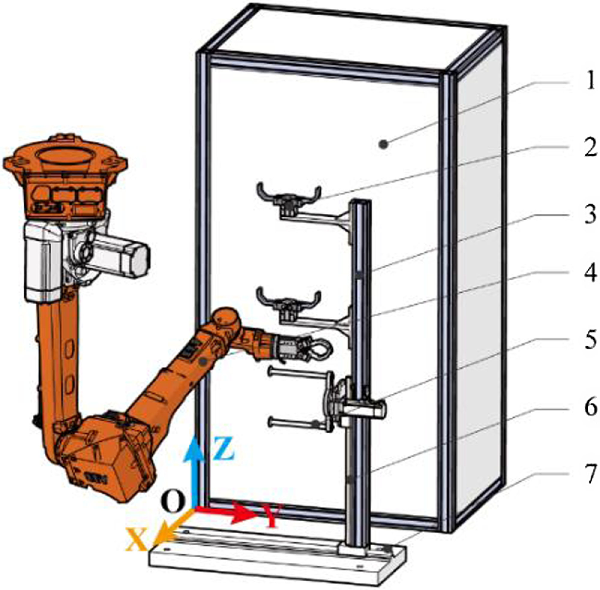
Figure 2. The simplified basic unit of the weaving system (1- yarn fixing unit; 2- yarn storage mechanism; 3- support rod; 4- robot; 5- yarn winding mechanism; 6- vertical sliding guide; 7- horizontal sliding guide; 8- obstacle mechanism).
Facing the challenge of meeting requirements using manual teaching, it is crucial to research a path planning method that works well for weaving robots. Considering the characteristics of the weaving system, the objectives and challenges of path planning are as follows:
-
1. The planned path must meet the requirements of yarn storage movements. The action of storing yarn by robots is complex, and each mechanism has its own unique storage path. Fig. 3 displays how the robot places yarn into the yarn storage mechanism 2 and the yarn winding mechanism 5, respectively. The curve shows the path of the robot storing yarn, and the arrow shows the direction of movement. Successful yarn storage can only be achieved by employing actions like lifting, avoiding obstacles, storing, and stretching.
-
2. The planned path should adapt to changes in the position of the mechanism. With the continuous weaving of the preform, the yarn storage mechanism 2 and the yarn winding mechanism 5 move along the guide rail according to a certain law. The winding mechanism 5 will move along the vertical sliding guide rail 6, which changes the Z value; the support rod 3 moves along the horizontal sliding guide rail 7, driving the change of Y value of the yarn storage mechanism 2 and the yarn winding mechanism 5.
-
3. The planned path cannot collide with surrounding institutions. It is frequent to collide with surrounding storage mechanisms during path planning due to the narrow workspace of the robot, which increases the difficulty of path planning.
3. ELM-IRRT path planning method
According to the path planning requirements of the weaving robot, the path planning method, namely ELM-IRRT, is proposed as shown in Fig. 4, which is composed of the teaching and learning phase and the expansion phase. The LfD phase employs ELM to establish a mapping relationship between the starting and ending points and path points, allowing for the learning of various paths of yarn storage. The starting and ending points of current task are input into the mapping relationship to obtain an imitation path with similar yarn storage action.
Table I. D-H parameter of robotic arm.


Figure 3. Yarn storage process for two mechanisms. (a) Yarn storage process for yarn storage mechanism 2, (b) yarn storage process for yarn winding mechanism 5.

Figure 4. The principle of the ELM-IRRT path planning method.
In the second expansion phase, the spatial guidance points can be extracted from imitation path, which are used to guide the expansion of the path in joint space (6-dimensional space for the weaving robot). The IRRT method with adaptive direction and step size is proposed to realize path planning in joint space. The expansion direction of the tree nodes is biased toward the spatial guide points to maintain a similar path shape. At the same time, based on the obstacle avoidance ability of IRRT, each node in the three-dimensional space does not collide with obstacles, and each linkage of the robot does not collide with obstacles. Finally, the collision-free path satisfying the yarn storage action is obtained in the form of robot joint data.
3.1. The LfD phase
3.1.1. Task demonstration and data collection
In the task demonstration, the yarn storage paths of the two mechanisms at different starting points
 $(X_{\textit{start}},Y_{\textit{start}},Z_{\textit{start}})$
and ending points
$(X_{\textit{start}},Y_{\textit{start}},Z_{\textit{start}})$
and ending points
 $(X_{end},Y_{end},Z_{end})$
are taught. Each path is composed of a sequence of path points
$(X_{end},Y_{end},Z_{end})$
are taught. Each path is composed of a sequence of path points
 $(x_{i},y_{i},z_{i})$
. Collect teaching data for storing yarn process in yarn storage mechanism 2 and yarn winding mechanism 5. First, B-spline interpolation is used to convert the sparse path points into rich training data due to the sparsity of teaching path points. Second, split the coordinate values according to the coordinate direction and normalize them to obtain the coordinate sequences
$(x_{i},y_{i},z_{i})$
. Collect teaching data for storing yarn process in yarn storage mechanism 2 and yarn winding mechanism 5. First, B-spline interpolation is used to convert the sparse path points into rich training data due to the sparsity of teaching path points. Second, split the coordinate values according to the coordinate direction and normalize them to obtain the coordinate sequences
 $t_{x}, t_{y}$
, and
$t_{x}, t_{y}$
, and
 $t_{z}$
for the directions
$t_{z}$
for the directions
 $x, y$
, and
$x, y$
, and
 $z$
, respectively. Finally, the training samples
$z$
, respectively. Finally, the training samples
 $D_{x}=\{X,t_{x}\}, D_{y}=\{Y,t_{y}\}$
and
$D_{x}=\{X,t_{x}\}, D_{y}=\{Y,t_{y}\}$
and
 $D_{z}=\{Z,t_{z}\}$
for each coordinate are composed, where
$D_{z}=\{Z,t_{z}\}$
for each coordinate are composed, where
 $X, Y$
, and
$X, Y$
, and
 $Z$
are the sets of starting and ending points in the x, y, and z directions, respectively.
$Z$
are the sets of starting and ending points in the x, y, and z directions, respectively.
3.1.2. Network model training by ELM
ELM has high learning accuracy and less network training time, and its output is that
 \begin{equation} t_{zj}=o=\sum _{i=1}^{L}\beta _{i}f_{i}\!\left(Z_{j}\right)=\sum _{i=1}^{L}\beta _{i}g\!\left(W_{i}^{T}Z_{j}+b_{i}\right),j=1,\ldots,N \end{equation}
In Eq. (1), L represents the number of hidden nodes, N represents the number of training samples, and
 $g(x)$
represents the activation function.
$g(x)$
represents the activation function.
 $W_{i}=[w_{i,1},w_{i,2}]$
is the weight vector connecting the ith hidden node and the input node,
$W_{i}=[w_{i,1},w_{i,2}]$
is the weight vector connecting the ith hidden node and the input node,
 $\beta _{i}=[\beta _{i,1},\beta _{i,2},\ldots,\beta _{i,m}]$
is the weight vector connecting the ith hidden node and the output node, and
$\beta _{i}=[\beta _{i,1},\beta _{i,2},\ldots,\beta _{i,m}]$
is the weight vector connecting the ith hidden node and the output node, and
 $b_{i}$
is the deviation of hidden layer. The values of
$b_{i}$
is the deviation of hidden layer. The values of
 $W_{i}$
and
$W_{i}$
and
 $b_{i}$
are randomly given during the training process, and the minimum square method is used to minimize the error of the output result
$b_{i}$
are randomly given during the training process, and the minimum square method is used to minimize the error of the output result
 \begin{equation} \min \!\left(H\beta ^{T}-T\right) \end{equation}
 \begin{equation} H\!\left(W,Z,b\right)=\left[\begin{array}{c@{\quad}c@{\quad}c} g\!\left(w_{1}^{T}Z_{1}+b_{1}\right) & \ldots & g\!\left(w_{L}^{T}Z_{1}+b_{L}\right)\\ \ldots & \ldots & \ldots \\ g\!\left(w_{1}^{T}Z_{N}+b_{1}\right) & \ldots & g\!\left(w_{L}^{T}Z_{N}+b_{L}\right) \end{array}\right]\in R^{N\times L} \end{equation}
In Eq. (2),
 $H$
is the hidden layer output matrix,
$H$
is the hidden layer output matrix,
 $\beta$
is obtained from
$\beta$
is obtained from
 $\hat{\beta }^{T}=H^{\dagger }T$
where
$\hat{\beta }^{T}=H^{\dagger }T$
where
 $H^{\dagger }$
is the Moore–Penrose generalized inverse matrix of matrix
$H^{\dagger }$
is the Moore–Penrose generalized inverse matrix of matrix
 $H$
.
$H$
.
The ELM network model is trained by training samples
 $D_{x}=\{X,t_{x}\}, D_{y}=\{Y,t_{y}\}$
, and
$D_{x}=\{X,t_{x}\}, D_{y}=\{Y,t_{y}\}$
, and
 $D_{z}=\{Z,t_{z}\}$
to obtain the mapping relationships of
$D_{z}=\{Z,t_{z}\}$
to obtain the mapping relationships of
 $f_{x}\colon X\rightarrow t_{x}, f_{y}\colon Y\rightarrow t_{y}$
, and
$f_{x}\colon X\rightarrow t_{x}, f_{y}\colon Y\rightarrow t_{y}$
, and
 $f_{z}\colon Z\rightarrow t_{z}$
. The training framework of ELM is shown in Fig. 5.
$f_{z}\colon Z\rightarrow t_{z}$
. The training framework of ELM is shown in Fig. 5.
 $X$
remains unchanged since there is no guide rail in the x direction,
$X$
remains unchanged since there is no guide rail in the x direction,
 $f_{x}=t_{x}$
; the independent variable of
$f_{x}=t_{x}$
; the independent variable of
 $f_{y}$
is
$f_{y}$
is
 $Y_{end}$
since the starting point of the system path is located at the vertical centerline of yarn fixing unit 1; and the independent variables of
$Y_{end}$
since the starting point of the system path is located at the vertical centerline of yarn fixing unit 1; and the independent variables of
 $f_{z}$
are
$f_{z}$
are
 $Z_{\textit{start}}$
and
$Z_{\textit{start}}$
and
 $Z_{end}$
.
$Z_{end}$
.

Figure 5. Training framework of ELM.
3.1.3. The output of imitation path
According to the position of the mechanism on the vertical sliding guide rail 6 or horizontal sliding guide rail 7, input the starting point
 $(x_{\textit{start}},y_{\textit{start}},z_{\textit{start}})$
and ending point
$(x_{\textit{start}},y_{\textit{start}},z_{\textit{start}})$
and ending point
 $(x_{end},y_{end},z_{end})$
into the mapping relationship to obtain the imitation path
$(x_{end},y_{end},z_{end})$
into the mapping relationship to obtain the imitation path
 $(t'_{x},t'_{y},t'_{z})$
that resembles the yarn storage actions in the teaching path.
$(t'_{x},t'_{y},t'_{z})$
that resembles the yarn storage actions in the teaching path.
3.2. Expansion phase
3.2.1. Collision detection
In order to accurately describe the robot and obstacle models, three envelope types of capsule, sphere, and cuboid are used to envelop the basic weaving unit. The algebraic method in literature [Reference Kong and Yu38] can be used to quickly realize the collision detection between capsule and capsule, capsule and sphere, and sphere and sphere. However, the collision detection between cuboid and capsule and between cuboid and sphere is more complicated. In such cases, the capsule and sphere need to be converted into convex multilateral bodies, and then GJK algorithm [Reference v. d. Bergen39] can be used to detect the collision. The capsule body can be regarded as a combination of cylinder and hemisphere, as shown in Fig. 6. Similarly, the sphere is a combination of two hemispheres, and the outer tangential support point of the cylinder and hemisphere is the vertex of the convex multilateral body.

Figure 6. Convex multilateral body converted from cylinder and sphere transformation.
A circumscribed prism with n edges is created on a cylinder with a radius of
 $r_{c}$
. The coordinates of the support points of the cylinder are expressed as
$r_{c}$
. The coordinates of the support points of the cylinder are expressed as
 \begin{equation} {}^{c}{C}{_{ij}^{}}=A_{i}+\frac{r_{c}}{\cos \theta }\!\left[\cos \!\left(2\!\left(j-1\right)\theta \right),\sin \!\left(2\!\left(j-1\right)\theta \right),0\right],\,i=1,2;\ j=1,2,\ldots,n \end{equation}
In Eq. (4),
 $\theta =\pi /\mathrm{n}$
. For a sphere with radius
$\theta =\pi /\mathrm{n}$
. For a sphere with radius
 $r_{s}$
, the vertices of outer tangent polygon for m parallel circles are taken as the support points of the sphere, which are expressed as
$r_{s}$
, the vertices of outer tangent polygon for m parallel circles are taken as the support points of the sphere, which are expressed as
 \begin{equation} {}^{s}{S}{_{ij}^{}}=O_{i}+\frac{r_{i}}{\cos \theta }\!\left[\cos \!\left(2\!\left(j-1\right)\theta \right),\sin \!\left(2\!\left(j-1\right)\theta \right),0\right],\,i=1,2,\ldots,m;\ j=1,2,\ldots,n \end{equation}
In Eq. (5),
 $O_{i}=\left[0,0,h_{i}\right], h_{i}=\frac{i}{m+1}r_{s}$
, and
$O_{i}=\left[0,0,h_{i}\right], h_{i}=\frac{i}{m+1}r_{s}$
, and
 $r_{i}=\sqrt{r_{s}^{2}-h_{i}^{2}}$
. In order to detect the collision, a conversion process is carried out on the coordinates from
$r_{i}=\sqrt{r_{s}^{2}-h_{i}^{2}}$
. In order to detect the collision, a conversion process is carried out on the coordinates from
 $\{O_{c}\}$
to
$\{O_{c}\}$
to
 $\{O_{b}\}$
and
$\{O_{b}\}$
and
 $\{O_{s}\}$
to
$\{O_{s}\}$
to
 $\{O_{b}\}$
, obtaining the support points
$\{O_{b}\}$
, obtaining the support points
 ${}^{b}{C}{_{ij}^{}}$
and
${}^{b}{C}{_{ij}^{}}$
and
 ${}^{b}{S}{_{ij}^{}}$
. The GJK algorithm is then utilized for the collision detection of cuboid and sphere.
${}^{b}{S}{_{ij}^{}}$
. The GJK algorithm is then utilized for the collision detection of cuboid and sphere.
A detection queue is formed by the envelope of all obstacles. The method for collision detection is chosen based on the type of envelope to detect collision with each linkage of the robot individually. If there is any collision between the envelope of obstacle and the envelope of robot linkage, it will be flagged as a collision. Fig. 7 illustrates the basic weaving unit enveloped by capsule, sphere, and cube envelope.

Figure 7. The basic weaving unit enveloped by capsule, sphere, and cube envelope.
3.2.2. IRRT algorithm
The RRT algorithm is a path planning method based on random sampling. The classic RRT algorithm first constructs a tree with the root node as the starting point in the joint space. Then a random point
 $q_{rand}$
is generated in the joint space, and the node
$q_{rand}$
is generated in the joint space, and the node
 $q_{near}$
closest to
$q_{near}$
closest to
 $q_{rand}$
is found through traversing the tree. As the parent node,
$q_{rand}$
is found through traversing the tree. As the parent node,
 $q_{near}$
expand a step along the
$q_{near}$
expand a step along the
 $q_{rand}$
direction to generate a new node
$q_{rand}$
direction to generate a new node
 $q_{new}$
. Finally, the each link position of the robot in
$q_{new}$
. Finally, the each link position of the robot in
 $q_{new}$
is calculated to detect the collision. If the collision occurs, the point is discarded, otherwise,
$q_{new}$
is calculated to detect the collision. If the collision occurs, the point is discarded, otherwise,
 $q_{new}$
is added to the tree. If the distance between
$q_{new}$
is added to the tree. If the distance between
 $q_{new}$
and
$q_{new}$
and
 $q_{goal}$
is less than the set threshold, the path expansion is successful. The above process is repeated until the expansion is successful or the number of iterations is exceeded.
$q_{goal}$
is less than the set threshold, the path expansion is successful. The above process is repeated until the expansion is successful or the number of iterations is exceeded.
The expansion process of the basic RRT algorithm is time consuming to converge to the target point in high-dimensional space. In addition, the step length of the joint space movement requires repeated trial and error processes. For this reason, as shown in Fig. 8, an improved RRT algorithm with adaptive direction and step size, namely the IRRT algorithm, is proposed to improve path quality.

Figure 8. Schematic diagram of IRRT.
(1) Adaptive direction.
The adaptive direction aims to synthesize the expansion direction according to the target gravitational vector and the random gravitational vector. The directions of the target gravitational vector and the random gravitational vector are determined by the target point and the random sampling point, respectively. The gravitational force of
 $q_{goal}$
is defined as
$q_{goal}$
is defined as
 $F_{goal}$
, and the gravitational force of
$F_{goal}$
, and the gravitational force of
 $q_{rand}$
is defined as
$q_{rand}$
is defined as
 $F_{rand}$
. The expansion direction is defined as
$F_{rand}$
. The expansion direction is defined as
 \begin{equation} \boldsymbol{n}=F_{rand}\!\left(\frac{q_{rand}-q_{near}}{\left\| q_{rand}-q_{near}\right\| }\right)+F_{goal}\!\left(\frac{q_{\textit{orient}}-q_{near}}{\left\| q_{\textit{orient}}-q_{near}\right\| }\right) \end{equation}
Taking the expansion failures number
 $N_{\textit{failed}}$
of its parent node as the independent variable, the new functions of
$N_{\textit{failed}}$
of its parent node as the independent variable, the new functions of
 $F_{rand}$
and
$F_{rand}$
and
 $F_{goal}$
are defined as
$F_{goal}$
are defined as
 \begin{equation} F_{rand}=e^{\frac{N_{\textit{failed}}}{2}}-1,\,F_{goal}=e^{{-^{\frac{N_{\textit{failed}}}{2}}}} \end{equation}
The initial value of
 $N_{\textit{failed}}$
is zero, and
$N_{\textit{failed}}$
is zero, and
 $N_{\textit{failed}}$
is accumulated once when a collision is detected during expansion or the joint value exceeds the joint range. It can be seen from Eq. (7) that
$N_{\textit{failed}}$
is accumulated once when a collision is detected during expansion or the joint value exceeds the joint range. It can be seen from Eq. (7) that
 $\boldsymbol{n}$
is toward the target point and the new point directly is expanded toward the target point when
$\boldsymbol{n}$
is toward the target point and the new point directly is expanded toward the target point when
 $N_{\textit{failed}}=0$
. The greater the number of
$N_{\textit{failed}}=0$
. The greater the number of
 $N_{\textit{failed}}$
, the greater the value of
$N_{\textit{failed}}$
, the greater the value of
 $F_{rand}$
, and the smaller the value of
$F_{rand}$
, and the smaller the value of
 $F_{goal}$
. Then the overall expansion direction tends to be more random. The new point after expansion is
$F_{goal}$
. Then the overall expansion direction tends to be more random. The new point after expansion is
 \begin{equation} q_{new}=q_{near}+\textit{stepsize}\frac{\boldsymbol{n}}{\left\| \boldsymbol{n}\right\| } \end{equation}
In Eq. (8), stepsize represents the step size of expansion, and its value is calculated by the adaptive step size method.
(2) Adaptive step size.
According to the current expansion direction and joint values, the adaptive step size of the joint space is obtained to ensure that the maximum movement distance of each joint is less than the minimum obstacle width. The Jacobian matrix reflects the influence of small changes in joint angles on the speed of the end effector in the form of
 \begin{equation}\mathit{v} = [{\mathit{w}_{\mathit{x}}}\mathit{,}{\mathit{w}_{\mathit{y}}}{\mathit{,}\mathit{w}_{\mathit{z}}}\mathit{,}{\mathit{v}_{\mathit{x}}}\mathit{,}{\mathit{v}_{\mathit{y}}}\mathit{,}{\mathit{v}_{\mathit{z}}}]^{\mathit{T}} = \mathit{J}(\mathit{q})\dot{\mathit{q}} \end{equation}
In Eq. (9),
 $J(q)$
represents the geometric Jacobian matrix, and
$J(q)$
represents the geometric Jacobian matrix, and
 $\mathit{v}$
represents the spatial velocity composed of angular velocity
$\mathit{v}$
represents the spatial velocity composed of angular velocity
 $w$
and linear velocity
$w$
and linear velocity
 $v$
. Set
$v$
. Set
 $J(q)=[J_{w}(q),J_{v}(q)]^{T}$
, then the linear velocity of the
$J(q)=[J_{w}(q),J_{v}(q)]^{T}$
, then the linear velocity of the
 $i-\mathrm{th}$
joint can be expressed as
$i-\mathrm{th}$
joint can be expressed as
 \begin{equation}\dot{\mathit{p}}_{\mathit{i}} = [{\mathit{v}_{\mathit{xi}}}\mathit{,}{\mathit{v}_{\mathit{yi}}}\mathit{,}{\mathit{v}_{\mathit{zi}}}]^{\mathit{T}} = \mathit{J}_{\mathit{vi}}\!\left(\dot{\mathit{q}}_{\mathit{i}}\right),\mathit{i}=1,2,\ldots,6 \end{equation}
In Eq. (10),
 $\dot{\mathit{p}}_{\mathit{i}}$
represents the linear velocity of the
$\dot{\mathit{p}}_{\mathit{i}}$
represents the linear velocity of the
 $i$
th joint,
$i$
th joint,
 $\dot{\mathit{q}}_{\mathit{i}}=[{\dot{\mathit{\theta }}_{1}},\ldots,{\dot{\mathit{\theta }}_{\mathit{i}}}]^{\mathit{T}}\in \mathit{R}^{\mathit{i}\times 1}$
, and
$\dot{\mathit{q}}_{\mathit{i}}=[{\dot{\mathit{\theta }}_{1}},\ldots,{\dot{\mathit{\theta }}_{\mathit{i}}}]^{\mathit{T}}\in \mathit{R}^{\mathit{i}\times 1}$
, and
 $J_{vi}(q)\in R^{3\times i}$
represents the linear velocity Jacobian matrix that regards ith joint as terminal joint, which is related to the rotation angle of the first i joint.
$J_{vi}(q)\in R^{3\times i}$
represents the linear velocity Jacobian matrix that regards ith joint as terminal joint, which is related to the rotation angle of the first i joint.
After obtaining the
 $\boldsymbol{n}$
by Eq. (6), the maximum step length in this direction is found: set
$\boldsymbol{n}$
by Eq. (6), the maximum step length in this direction is found: set
 $n_{j} = \max (| n_{1},\ldots,n_{i}| )$
where
$n_{j} = \max (| n_{1},\ldots,n_{i}| )$
where
 $j$
is the maximum subscript. Assume that each joint reaches a new point at the same time, that is,
$j$
is the maximum subscript. Assume that each joint reaches a new point at the same time, that is,
 $\dot{\mathit{\theta }}_{1}\colon \dot{\mathit{\theta }}_{2}\colon \ldots \colon \dot{\mathit{\theta }}_{\mathit{i}} = \mathit{n}_{1}\colon \mathit{n}_{2}\colon \ldots \colon \mathit{n}_{\mathit{i}}$
, then
$\dot{\mathit{\theta }}_{1}\colon \dot{\mathit{\theta }}_{2}\colon \ldots \colon \dot{\mathit{\theta }}_{\mathit{i}} = \mathit{n}_{1}\colon \mathit{n}_{2}\colon \ldots \colon \mathit{n}_{\mathit{i}}$
, then
 $\dot{\mathit{q}}_{\mathit{i}} = [\frac{\mathit{n}_{1}}{\mathit{n}_{\mathit{j}}},\frac{\mathit{n}_{2}}{\mathit{n}_{\mathit{j}}},\ldots,\frac{\mathit{n}_{\mathit{i}}}{\mathit{n}_{\mathit{j}}}]^{\mathit{T}}\dot{\mathit{\theta }}_{\mathit{j}}$
is substituted into Eq. (10). Multiply both sides by
$\dot{\mathit{q}}_{\mathit{i}} = [\frac{\mathit{n}_{1}}{\mathit{n}_{\mathit{j}}},\frac{\mathit{n}_{2}}{\mathit{n}_{\mathit{j}}},\ldots,\frac{\mathit{n}_{\mathit{i}}}{\mathit{n}_{\mathit{j}}}]^{\mathit{T}}\dot{\mathit{\theta }}_{\mathit{j}}$
is substituted into Eq. (10). Multiply both sides by
 $\Delta t$
to get that
$\Delta t$
to get that
 \begin{equation} \Delta p_{i}=J_{vi}\!\left(q_{i}\right)\left[\frac{n_{1}}{n_{j}},\frac{n_{2}}{n_{j}},\ldots,\frac{n_{i}}{n_{j}}\right]^{T}\Delta \theta _{j} \end{equation}
In order to simplify the expression, let
 $\Delta p_{i}=A_{i}\Delta \theta _{j}$
. It can be seen that
$\Delta p_{i}=A_{i}\Delta \theta _{j}$
. It can be seen that
 $A_{i}$
is related to the expansion direction
$A_{i}$
is related to the expansion direction
 $\boldsymbol{n}$
and the rotation angle of the first
$\boldsymbol{n}$
and the rotation angle of the first
 $i$
joint. Use the compatibility of the norm
$i$
joint. Use the compatibility of the norm
 $\| Ax\| \leq \| A\| \, \| x\|$
to get that
$\| Ax\| \leq \| A\| \, \| x\|$
to get that
 \begin{equation} \left\| \Delta p_{i}\right\| \leq \left\| A_{i}\right\| \left\| \Delta \theta _{j}\right\| \end{equation}
Since
 $\| \Delta p_{i}\| _{2}=\sqrt{\Delta p_{ix}^{2}+\Delta p_{iy}^{2}+\Delta p_{iz}^{2}}$
represents the distance that ith linkage moves in Cartesian space, the 2 norm is selected for the Eq. (12). Suppose the width of the smallest obstacle in the working space is
$\| \Delta p_{i}\| _{2}=\sqrt{\Delta p_{ix}^{2}+\Delta p_{iy}^{2}+\Delta p_{iz}^{2}}$
represents the distance that ith linkage moves in Cartesian space, the 2 norm is selected for the Eq. (12). Suppose the width of the smallest obstacle in the working space is
 $\nabla$
, that is, the maximum value on the right side of Eq. (12) is
$\nabla$
, that is, the maximum value on the right side of Eq. (12) is
 $\nabla$
. We can get that
$\nabla$
. We can get that
 \begin{equation} \left\| \Delta p_{i,\max }\right\| _{2}\leq \max \!\left\| A_{i}\right\| _{2}\left\| \Delta \theta _{j}\right\| _{2}=\nabla \end{equation}
 \begin{equation} \Delta \theta _{j}=\left\| \Delta \theta _{j}\right\| _{2}=\frac{\nabla }{\max \!\left\| A_{i}\right\| _{2}} \end{equation}
From Eq. (14), the maximum expansion step in the
 $\boldsymbol{n}$
direction is calculated as
$\boldsymbol{n}$
direction is calculated as
 \begin{equation} \textit{Stepsize}=\frac{\Delta \theta _{j}}{n_{j}} \end{equation}
The distance of movement of the linkage of the robot is less than the width of the minimum obstacle under the step size.
3.2.3. Expansion of path points
The imitation path obtained in section 3.1 cannot guarantee that each joint of robot does not collide with the surrounding mechanism in the narrow space. Therefore, the path point expansion method is designed based on the advantage of fast expansion without collision in IRRT. Regarding the spatial guidance points of imitation path as theguidance for IRRT, the path shape of the yarn storage is obtained by expending along the guiding path when there is no collision. The expansion angle is adjusted continuously to ensure that each linkage of the robot does not collide with surrounding mechanisms when there is collision. The principle of path points expansion is shown in Fig. 9.

Figure 9. Schematic diagram of path point expansion.
(1) After inserting
 $m$
path points uniformly between the imitation path points, the initial pose and end pose are interpolated and the inverse kinematics of the robot is solved. The obtained joint data
$m$
path points uniformly between the imitation path points, the initial pose and end pose are interpolated and the inverse kinematics of the robot is solved. The obtained joint data
 $\textit{Orient}\{i\}=[q_{1},q_{2},\ldots,q_{6}]$
are used as the spatial guidance points for the expansion point where
$\textit{Orient}\{i\}=[q_{1},q_{2},\ldots,q_{6}]$
are used as the spatial guidance points for the expansion point where
 $i=1,2,\ldots,m$
. The spatial guidance point is the instantaneous target point of IRRT, which leads IRRT to expand along the imitation path.
$i=1,2,\ldots,m$
. The spatial guidance point is the instantaneous target point of IRRT, which leads IRRT to expand along the imitation path.
(2) Random sampling is conducted within the angle range of the robot to obtain sampling point
 $q_{rand}$
and a random number is generated between 0 and 1. If the random number is less than 0.9, the index
$q_{rand}$
and a random number is generated between 0 and 1. If the random number is less than 0.9, the index
 $i_{\textit{closest}}$
of the guidance point closest to the end of the expansion tree is found and
$i_{\textit{closest}}$
of the guidance point closest to the end of the expansion tree is found and
 $q_{\textit{orient}}=\textit{Orient}\{i_{\textit{closest}}+1\}$
is regarded as the target point
$q_{\textit{orient}}=\textit{Orient}\{i_{\textit{closest}}+1\}$
is regarded as the target point
 $q_{goal}$
for this expansion. The node
$q_{goal}$
for this expansion. The node
 $q_{near}$
closest to
$q_{near}$
closest to
 $q_{goal}$
is defined as the parent node; otherwise, the node
$q_{goal}$
is defined as the parent node; otherwise, the node
 $q_{near}$
closest to
$q_{near}$
closest to
 $q_{rand}$
is defined as the parent node. The index
$q_{rand}$
is defined as the parent node. The index
 $i_{\textit{closest}}$
of the guidance point closest to the
$i_{\textit{closest}}$
of the guidance point closest to the
 $q_{near}$
is calculated, and
$q_{near}$
is calculated, and
 $q_{\textit{orient}}=\textit{Orient}\{i_{\textit{closest}}+1\}$
is used as the target point
$q_{\textit{orient}}=\textit{Orient}\{i_{\textit{closest}}+1\}$
is used as the target point
 $q_{goal}$
of this expansion.
$q_{goal}$
of this expansion.
(3) IRRT algorithm is used to calculate the expansion direction and step size, and the new node
 $q_{new}$
is calculated.
$q_{new}$
is calculated.
(4) Collision detection is carried out at the angle of
 $q_{new}$
. If there is a collision or joint is out of range,
$q_{new}$
. If there is a collision or joint is out of range,
 $N_{\textit{failed}}=N_{\textit{failed}}+1$
, and return step (2). Otherwise,
$N_{\textit{failed}}=N_{\textit{failed}}+1$
, and return step (2). Otherwise,
 $q_{new}$
is expanded on the parent node
$q_{new}$
is expanded on the parent node
 $q_{near}$
(to speed up the convergence speed, this paper defines that when the
$q_{near}$
(to speed up the convergence speed, this paper defines that when the
 $N_{\textit{failed}}$
>50 for this parent node, it will not generate a new node).
$N_{\textit{failed}}$
>50 for this parent node, it will not generate a new node).
(5) The distance between
 $q_{new}$
and
$q_{new}$
and
 $q_{end}$
is calculated. If it is less than the threshold, the path expansion is successful. Otherwise, steps (2)–(5) will be repeated until the maximum number of iterations is reached.
$q_{end}$
is calculated. If it is less than the threshold, the path expansion is successful. Otherwise, steps (2)–(5) will be repeated until the maximum number of iterations is reached.
Sharp path points reduce the stability of the robot movement and a smooth path is required. The principle of smooth path is shown in Fig. 10. Suppose that
 $p_{i+1}$
is a sharp point when
$p_{i+1}$
is a sharp point when
 $\angle p_{i+1}p_{i}p_{i+2}\gt 30^{\circ}$
and
$\angle p_{i+1}p_{i}p_{i+2}\gt 30^{\circ}$
and
 $p_{i+1}$
is deleted if there are no obstacles between
$p_{i+1}$
is deleted if there are no obstacles between
 $p_{i}$
and
$p_{i}$
and
 $p_{i+2}$
.
$p_{i+2}$
.
 $p_{1}p_{2}p_{3}p_{4}p_{5}p_{6}$
is an unsmoothed path.
$p_{1}p_{2}p_{3}p_{4}p_{5}p_{6}$
is an unsmoothed path.
 $\angle p_{2}p_{1}p_{3}\gt 30^{\circ}, p_{2}$
is a sharp point. Since there is no obstacle between
$\angle p_{2}p_{1}p_{3}\gt 30^{\circ}, p_{2}$
is a sharp point. Since there is no obstacle between
 $p_{1}$
and
$p_{1}$
and
 $p_{3}, p_{2}$
is deleted;
$p_{3}, p_{2}$
is deleted;
 $\angle p_{5}p_{4}p_{6}\gt 30^{\circ}$
and
$\angle p_{5}p_{4}p_{6}\gt 30^{\circ}$
and
 $p_{5}$
is a sharp point. Since there is no obstacle between
$p_{5}$
is a sharp point. Since there is no obstacle between
 $p_{4}$
and
$p_{4}$
and
 $p_{6}, p_{5}$
is reserved. The smoothed path is
$p_{6}, p_{5}$
is reserved. The smoothed path is
 $p_{1}p_{3}p_{4}p_{5}p_{6}$
. Based on this, a smooth path method is designed.
$p_{1}p_{3}p_{4}p_{5}p_{6}$
. Based on this, a smooth path method is designed.

Figure 10. Schematic diagram of smooth path.
(1) The distance between point
 $p_{i}$
and point
$p_{i}$
and point
 $p_{i+1}$
is record as
$p_{i+1}$
is record as
 $d_{i,i+1}$
. The initial value of
$d_{i,i+1}$
. The initial value of
 $i$
is 1, and
$i$
is 1, and
 $d_{i,i+1},d_{i,i+2},d_{i+1,i+2}$
is calculated.
$d_{i,i+1},d_{i,i+2},d_{i+1,i+2}$
is calculated.
(2) Determine whether
 $p_{i+1}$
is a sharp point. If
$p_{i+1}$
is a sharp point. If
 $d_{i,i+2}+\delta \lt d_{i+1,i+2}+d_{i,i+1}, p_{i+1}$
is a sharp point, and m points are inserted uniformly between
$d_{i,i+2}+\delta \lt d_{i+1,i+2}+d_{i,i+1}, p_{i+1}$
is a sharp point, and m points are inserted uniformly between
 $p_{i}$
and
$p_{i}$
and
 $p_{i+2}$
for collision detection, and then enter step (3). Otherwise,
$p_{i+2}$
for collision detection, and then enter step (3). Otherwise,
 $p_{i+1}$
is not a sharp point, and let
$p_{i+1}$
is not a sharp point, and let
 $i=i+1$
, steps (1) and (2) are repeated. Among them,
$i=i+1$
, steps (1) and (2) are repeated. Among them,
 $\delta =2(\nabla -\nabla \cos 30^{\circ})$
, where
$\delta =2(\nabla -\nabla \cos 30^{\circ})$
, where
 $\nabla$
is the width of the minimum obstacle, and
$\nabla$
is the width of the minimum obstacle, and
 $m=\text{ceil}\!\left(\frac{d_{i,\,i+2}}{\nabla }\right)$
where ceil is a round-up function.
$m=\text{ceil}\!\left(\frac{d_{i,\,i+2}}{\nabla }\right)$
where ceil is a round-up function.
(3) If there is no collision, delete the point
 $i+1$
. Otherwise, let
$i+1$
. Otherwise, let
 $i=i+1$
and repeat the process of (1) (2) (3).
$i=i+1$
and repeat the process of (1) (2) (3).
4. Experiments and result analysis
4.1. LfD phase evaluation
To verify the effectiveness of the imitation paths obtained during the LfD phase, 12 paths with different starting and ending points were obtained by teaching the yarn storage path that mechanism 2 and the yarn winding mechanism 5 at different positions. Eight paths are randomly selected as the training set, and 4 paths are selected as the testing set. The number of hidden nodes is set to 1000, and the activation function is set to sigmoid function to train the network models in x, y, and z directions, respectively. After that, different starting and ending points were input to the trained model. The weaving system has no guide rail in the x direction, that is, the starting and ending points are fixed in the x direction. This means that
 $f_{x}$
has no independent variable, and the imitation path is the same as
$f_{x}$
has no independent variable, and the imitation path is the same as
 $t_{x}$
of teaching path; the path always starts at the vertical center line of yarn fixing unit 1, fixing the starting point in the y direction. Therefore,
$t_{x}$
of teaching path; the path always starts at the vertical center line of yarn fixing unit 1, fixing the starting point in the y direction. Therefore,
 $Y_{end}$
is the independent variable for
$Y_{end}$
is the independent variable for
 $f_{y}$
; The z direction has variable starting and ending points, with
$f_{y}$
; The z direction has variable starting and ending points, with
 $Z_{\textit{start}}$
and
$Z_{\textit{start}}$
and
 $Z_{\textit{start}}$
as the independent variables for
$Z_{\textit{start}}$
as the independent variables for
 $f_{z}$
. Fig 11
(a) shows the imitation results of the trained network model in y direction with different inputs of
$f_{z}$
. Fig 11
(a) shows the imitation results of the trained network model in y direction with different inputs of
 $Y_{end}$
, which is observed in the xoy plane. Fig. 11
(b) shows the imitation results of the trained network model in z direction with different inputs of
$Y_{end}$
, which is observed in the xoy plane. Fig. 11
(b) shows the imitation results of the trained network model in z direction with different inputs of
 $Z_{\textit{start}}$
and
$Z_{\textit{start}}$
and
 $Z_{end}$
, which is observed in the xoz plane. Fig. 12
(a) and 12(b) show the three-dimensional imitation paths of the yarn storage process of the yarn storage mechanism 2 and the yarn winding mechanism 5, respectively. From Figs. 11 and 12, it can be seen that the shape of the imitation path is consistent with the shape of the teaching path. Even if the starting and ending points that do not appear in the input teaching data are input, similar imitation paths can be obtained, indicating the effectiveness of the imitation path.
$Z_{end}$
, which is observed in the xoz plane. Fig. 12
(a) and 12(b) show the three-dimensional imitation paths of the yarn storage process of the yarn storage mechanism 2 and the yarn winding mechanism 5, respectively. From Figs. 11 and 12, it can be seen that the shape of the imitation path is consistent with the shape of the teaching path. Even if the starting and ending points that do not appear in the input teaching data are input, similar imitation paths can be obtained, indicating the effectiveness of the imitation path.

Figure 11. Result of learning from demonstration. (a) Imitated result of y-direction; (b) imitated result of z-direction.

Figure 12. The path of imitation in 3D space. (a) Paths of imitation for yarn storage mechanism 2; (b) path of imitation for yarn winding mechanism 5.
To demonstrate the reliability of the imitation path, the same starting and ending points as the test set are input into the network model to obtain the corresponding imitation path. The similarity between the imitation path and the test set path is quantitatively analyzed of using the sweep error area (SEA) defined in ref. [Reference Khansari-Zadeh and Billard40], where SEA is the area enclosed by the imitation path and the test set path. The smaller the area, the closer the imitation path and the test set path are. The SEA function is expressed as
 \begin{equation} E=\frac{1}{N}\sum _{n=1}^{N}\sum _{i=1}^{m-1}A\!\left(p\!\left(i\right),p\!\left(i+1\right),p_{demo}\!\left(i\right),p_{demo}\!\left(i+1\right)\right) \end{equation}
In Eq. (16),
 $A(p(i),p(i+1),p_{demo}(i),p_{demo}(i+1))$
represents the area of a quadrilateral surrounded by four points
$A(p(i),p(i+1),p_{demo}(i),p_{demo}(i+1))$
represents the area of a quadrilateral surrounded by four points
 $p(i), p(i+1), p_{demo}(i)$
and
$p(i), p(i+1), p_{demo}(i)$
and
 $p_{demo}(i+1)$
.
$p_{demo}(i+1)$
.
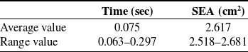
The performance of imitation path is shown in Table II. It can be seen from Table II that the corresponding imitation path is obtained in a relatively short time, and the mean value of SEA is 2.617 cm2. In other words, the area enclosed by the imitation path and the path of test set is small, indicating that the imitation path is close to the test set path so the simulated path has reliability.
Table II. Performance of imitation path.
4.2. IRRT algorithm evaluation
To verify the effectiveness of IRRT for obstacle avoidance, the performance of IRRT, Target-Gravity-RRT [Reference Cao, Zou, Jia, Chen and Zeng23] and GO-RRT [Reference Kang, Kim, Lee, Oh, You and Choi41] were compared in the same starting point, endpoint, and obstacle environment. The step size of Target-Gravity-RRT and GO-RRT are set to 0.07 rad and the minimum obstacle width is equal to the diameter of the sphere 0.07m. It is defined that the number of iterations exceeds 500 or the number of expansion failures exceeds 100 as a planning failure. Fig. 13 shows the path planning results of the three algorithms. The nodes of Target-Gravity-RRT are unevenly distributed, and the distance between nodes near the endpoint of sharply increases in GO-RRT. Compared to Target-Gravity-RRT and GO-RRT, the adaptive step size feature of IRRT makes the distribution of path points more uniform.

Figure 13. Comparison of planning results of three algorithms. (a) IRRT; (b) target gravity RRT; (c) GO-RRT. The blue line represents the planned path, and the dots represent the locations of the nodes of the random tree mapped in cartesian space.
To further demonstrate the advantages of adaptive step size, the displacement of each linkage of robot is compared with adaptive step size and fixed step size of 0.07 rad. It can be seen from Fig. 14 that the displacement of the link changes sharply when expansion with a fixed step size so that the displacement of the linkage-6 and the end effector sometimes exceeds
 $\nabla$
; the corresponding step size is solved based on the current joint value and expansion direction when expanding with adaptive step size, which makes the displacement of each link of the robot does not exceed
$\nabla$
; the corresponding step size is solved based on the current joint value and expansion direction when expanding with adaptive step size, which makes the displacement of each link of the robot does not exceed
 $\nabla$
and ensures the uniformity of path points.
$\nabla$
and ensures the uniformity of path points.

Figure 14. The comparison between fix step size and adaptive step size. (a) Fixed step size; (b) adaptive step size.
The experiment is repeated 100 times for the three algorithms, and the performance of algorithms is shown in Table III. Target-Gravity-RRT and GO RRT have both 0.06 rad and 0.07 rad step size
 $\Delta q$
. The maximum link displacement
$\Delta q$
. The maximum link displacement
 $\| \Delta p_{\max }\| _{2}$
exceeds the minimum obstacle width
$\| \Delta p_{\max }\| _{2}$
exceeds the minimum obstacle width
 $\nabla$
under the two step size. Although
$\nabla$
under the two step size. Although
 $\| \Delta p_{\max }\| _{2}$
of 0.06 rad step size is smaller than that of 0.07 rad step size, the number of iterations and planning time of 0.06 rad step size significantly increase. Therefore, Target-Gravity-RRT and GO-RRT need to repeatedly adjust the step size based on the obstacle width to obtain reasonable planning results. The adaptive step size of IRRT ensures that the maximum linkage displacement
$\| \Delta p_{\max }\| _{2}$
of 0.06 rad step size is smaller than that of 0.07 rad step size, the number of iterations and planning time of 0.06 rad step size significantly increase. Therefore, Target-Gravity-RRT and GO-RRT need to repeatedly adjust the step size based on the obstacle width to obtain reasonable planning results. The adaptive step size of IRRT ensures that the maximum linkage displacement
 $\| \Delta p_{\max }\| _{2}$
does not exceed the minimum obstacle width
$\| \Delta p_{\max }\| _{2}$
does not exceed the minimum obstacle width
 $\nabla$
with fewer iterations and shorter planning time. Especially in multiobstacle environments, a relationship between the expansion direction and the number of collisions is constructed in IRRT, forming an adaptive direction and improving the avoidance ability for expansion direction toward obstacles. Compared to Target-Gravity-RRT and GO-RRT algorithms, IRRT has a higher planning success rate.
$\nabla$
with fewer iterations and shorter planning time. Especially in multiobstacle environments, a relationship between the expansion direction and the number of collisions is constructed in IRRT, forming an adaptive direction and improving the avoidance ability for expansion direction toward obstacles. Compared to Target-Gravity-RRT and GO-RRT algorithms, IRRT has a higher planning success rate.
4.3. Expansion phase evaluation
Guided by the spatial guide points of imitation path obtained in the LfD phase, the expansion phase of ELM-IRRT utilizes the expansion ability of IRRT to generate paths that match the path shape and are collision-free in the joint space. To verify the validity of the ELM-IRRT method in the expansion phase, the method is applied to the planar map shown in Fig. 15. The map has complex terrain containing many obstacles, large obstacles, and narrow gaps, and even some guidance points are located in obstacles, which brings challenges to path planning. Fig. 15 (a) and Fig. 15 (b) show the path planning results under two kind of guidance ways, respectively. The expansion direction of the tree nodes moves forward along the guide point. When large obstacles are encountered, nodes can gradually bypass the obstacles based on the expansion ability of the proposed method. At the same time, in the case that the guide point does not correctly cross the narrow gap, the proposed method can still find the correct exit through the narrow gap, avoid getting trapped in the local area, and finally successfully reach the end point. Therefore, the proposed method is validity.
Table III. The comparison of algorithm performance.
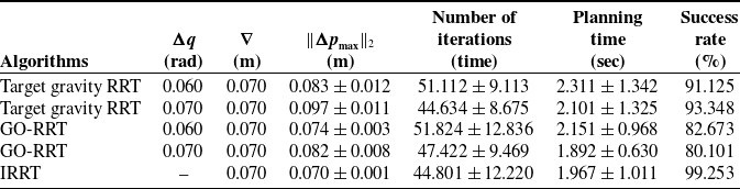

Figure 15. Path planning results in two-dimensional space under two kinds of guidance way. Green points represent guide points, green dotted lines represent the guidance way formed by guide points, blue points represent generated tree nodes, and red lines represent the final planned path.
To further verify the validity in high-dimensional space planning, the ELM-IRRT method is applied to a 7-DOF planar linkage robot with redundant degrees of freedom, where each link is 2.5 units long. The tree nodes expressed as the rotation angles of each joint are expanded in high-dimensional space. As shown in Fig. 16 (a), six sets of joint configures are given as spatial guidance points to guide the robot to move in an environment with two circular obstacles, and the path planning results of the proposed method are shown in Fig. 16 (b). In the case of collision between the linkage position configured by the guidance point and the obstacle, each linkage of the robot still bypassed the large obstacle, and the moving distance of each linkage did not exceed the size of the minimum obstacle to reached the target position. Therefore, the proposed method can obtain the joint data of the robot that conforms to the desired action, which is valid in the path planning of the high degree of freedom robot.

Figure 16. Path planning results of 7-DOF planar linkage robot. The black rings represent obstacles, and lines with different color represent robot with different joint configure.
4.4. An application example of path planning for a weaving robot
To test the ELM-IRRT path planning method, the weaving system is modeled in SolidWorks, teaching data is collected in Robot Studio, and the path planning strategy is programmed in MATLAB. The simulation test was run on a computer with a 2.3 GHz main frequency and 16 GB of memory. The ELM-IRRT method was validated for various yarn storage processes, and the experimental results are shown in Fig. 17.

Figure 17. Path planning results under different scenes. (a) Scene A; (b) Scene B; (c) Scene C; (d) Scene D.
Fig. 17 (a) shows the scene where the robot stores the yarn in the yarn storage mechanism 2. At this time, the LfD phase obtains an imitation path that does not collide with the surrounding mechanism. Since the path point does not collide with the surrounding mechanism, the path point expands directly to the target point in the expansion stage. This results in the imitation path being almost identical to the expansion path. In order to verify the obstacle avoidance ability in a complex obstacle environment, two obstacles are artificially added to the guidance point. The path planned by ELM-IRRT is shown in Fig. 17 (b). Since ELM-IRRT has the advantage of adaptive direction, the relationship between the extended direction and the number of collisions is constructed, avoiding the collision between the robot connecting rod and complex obstacles.
Fig. 17 (c) shows the scene where the robot stores the yarn into the winding mechanism 5. At this time, the LfD phase obtains an imitation path of collision with the surrounding mechanism. The collision-free path obtained in the expansion stage has some sharp points, and the path that is smooth and does not collide with the surrounding mechanism is obtained. Fig. 17 (d) illustrates the yarn winding mechanism 5 moving 0.2 m along the vertical guide rail 6 and 0.1 m along the horizontal guide rail 7. Despite the movement of the mechanism position, the path planned by the ELM-IRRT effectively meets the operation requirements of yarn storage while avoiding collision with the barriers.
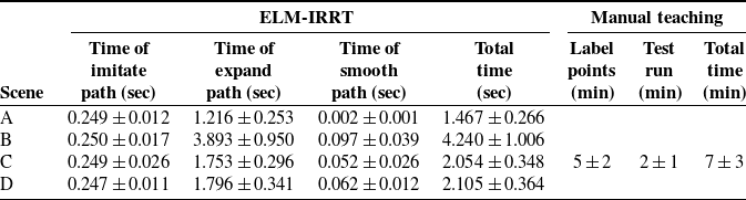
The experiment is repeated 30 times for the above yarn storage process, and the planning efficiency is shown in Table IV. The total time of path planning using ELM-IRRT method is within 2s–5s, while the time of traditional manual teaching path needs to be about 10 min. The path planning efficiency of using ELM-IRRT method for different yarn storage processes is much higher than that of manual teaching, further indicating that ELM-IRRT method has practical advantages on path planning of large weaving systems.
Table IV. Efficiency of path planning in different scenes.
5. Conclusion
Aiming at the path planning problem for robots in preform weaving, an ELM-IRRT path planning method is proposed. The main conclusions are as follows:
-
1. During the LfD phase of ELM-IRRT, ELM is used to autonomously learn the mapping relationship between the starting point, ending point, and path points. This process results in obtaining an imitation path with yarn storage action similar with the teaching path under different starting and ending points. The spatial guidance points of the imitation path are extracted to characterize the shape of the yarn storage process.
-
2. During the expansion phase of ELM-IRRT, the expansion direction of the tree node is inclined to the spatial guidance point of the imitation path, and each linkage of robot are guaranteed not to collide with obstacles in the moving process. Consequently, collision-free path with ideal shape was obtained in the joint space.
-
3. Based on the LfD and expansion phase, the path planned by the ELM-IRRT method not only meets the action requirements of yarn storage but also avoids the collision between the robot and the surrounding mechanisms. The proposed method can generate an ideal path within 2s–5s, avoiding the tedious manual teaching path, which is the practical and the feasible for path planning of the preform weaving robot.
Author contributions
All authors contributed to the study conception and design; Zhuo Meng conceived and designed the study; Material preparation and analysis were performed by Shuo Li; the first draft of the manuscript was written by Shuo Li and reviewed by Zhuo Meng; and the experiment data were collected by Yujing Zhang. The resources and equipment were provided by Yize Sun; all authors read and approved the final manuscript.
Financial support
This work is supported by Key R&D Program of Jiangsu Province (BE2023070).
Competing interests
The authors have no relevant financial or nonfinancial interests to disclose.


