


1. Introduction
Saltation, that is the motion of solid particles driven by a shearing flow in a gravitational field through successive jumps and rebounds from a base driven by a shearing flow, has been established as the main mode of transport of wind-blown sand (Bagnold Reference Bagnold1941; Owen Reference Owen1964; Andreotti Reference Andreotti2004; Charru, Andreotti & Claudin Reference Charru, Andreotti and Claudin2013; Valance et al. Reference Valance, Rasmussen, Ould El Moctar and Dupont2015) and is crucial to the dynamics of dunes (Sauermann, Kroy & Herrmann Reference Sauermann, Kroy and Herrmann2001). Although originally identified as the means of transport of sand grains by the wind on Earth, it has been recognized as significant also for the transport of sand or gravel in water on Earth (Fernandez Luque & Van Beek Reference Fernandez Luque and Van Beek1976; Abbott & Francis Reference Abbott and Francis1977; Niño & García Reference Niño and García1998; Ancey et al. Reference Ancey, Bigillon, Frey, Lanier and Ducret2002), basalt particles on Venus (Iversen & White Reference Iversen and White1982; Greeley et al. Reference Greeley, Iversen, Leach, Marshall, Williams and White1984) and Mars (Iversen et al. Reference Iversen, Pollack, Greeley and White1976; Iversen & White Reference Iversen and White1982), and ice particles on Titan (Burr et al. Reference Burr, Bridges, Marshall, Smith, White and Emery2015). While these studies considered the carrier fluid to be turbulent, saltation in viscous, non-turbulent fluids has also been investigated (Charru & Mouilleron-Arnould Reference Charru and Mouilleron-Arnould2002; Ouriemi, Aussillous & Guazzelli Reference Ouriemi, Aussillous and Guazzelli2009; Seizilles et al. Reference Seizilles, Lajeuness, Devauchelle and Bak2014), given its practical relevance in limiting the transport capacity of oil in pipes (Dall'Acqua et al. Reference Dall'Acqua, Benucci, Corvaro, Leporini, Cocci Grifoni, Del Monaco, Di Lullo, Passucci and Marchetti2017; Leporini et al. Reference Leporini, Terenzi, Marchetti, Corvaro and Polonara2019).
There is a large body of mathematical models of saltation in the literature (see, e.g. the reviews of Kok et al. Reference Kok, Parteli, Michaels and Karam2012; Valance et al. Reference Valance, Rasmussen, Ould El Moctar and Dupont2015; Pähtz et al. Reference Pähtz, Clark, Valyrakis and Durán2020). As highlighted by Valance et al. (Reference Valance, Rasmussen, Ould El Moctar and Dupont2015), the different models can be said to be Lagrangian or Eulerian, based upon the point of view adopted in the description of the particle motion.
In many Lagrangian approaches (Anderson et al. Reference Anderson, Haff, Anderson and Haff1988; Werner Reference Werner1990; Creyssels et al. Reference Creyssels, Dupont, Ould El Moctar, Valance, Cantat, Jenkins, Pasini and Rasmussen2009; Kok & Renno Reference Kok and Renno2009), particle trajectories are calculated from a distribution of the take-off velocities by solving the differential equations of their momentum balances, influenced by fluid drag and gravity, when immersed in a fluid with a prescribed velocity profile and for a given distribution of initial take-off velocity at the basal boundary. The calculation is repeated once the fluid velocity profile and the distribution of the take-off velocities are updated. This is done using a simple constitutive relation for the fluid shear stress (in the case of turbulent fluid, usually based on a mixing length approach) and a suitable set of boundary conditions that govern the impact of the particles at the base (Oger et al. Reference Oger, Ammi, Valance and Beladjine2005; Beladjine et al. Reference Beladjine, Ammi, Oger and Valance2007; Crassous, Beladjine & Valance Reference Crassous, Beladjine and Valance2007), until a steady state is attained.
Simpler Lagrangian approaches, in which the distribution of the particle trajectories is replaced by a single trajectory (Jenkins & Valance Reference Jenkins and Valance2014) or a pair of trajectories (Andreotti Reference Andreotti2004), have also been recently proposed and successfully compared against experiments and numerical simulations. In particular, the one trajectory models, also called periodic trajectory (PT) models, have been applied to saltation in both turbulent (Berzi, Jenkins & Valance Reference Berzi, Jenkins and Valance2016) and viscous (Pähtz et al. Reference Pähtz, Liu, Xia, Hu, He and Tholen2021; Valance & Berzi Reference Valance and Berzi2022) shearing flows, for values of the ratio of the grain-to-fluid mass densities encountered on Earth and other planetary bodies (Berzi, Valance & Jenkins Reference Berzi, Valance and Jenkins2017). The PT models are simple enough to allow for fully analytical solutions of steady and fully developed saltation, and permit rather accurate determination of global quantities, such as the particle mass flux, as a function of the intensity of the shearing flows. On the other hand, many variables of interest, such as the profile of the particle concentration and the total depth of the saltation layer, are poorly predicted. It is also not obvious how to extend this model to unsteady and/or inhomogeneous problems.
Another family of Lagrangian approaches is based on the framework of the discrete element method (DEM, Cundall & Strack Reference Cundall and Strack1979), and solves Newton's laws of motion for the individual grains that are allowed to collide with other particles and with the base, while the surrounding fluid is replaced by forces (such as drag and buoyancy) acting on the particles themselves (Tsuji, Kawaguchi & Tanaka Reference Tsuji, Kawaguchi and Tanaka1993). The corresponding forces transmitted by the particles on the fluid are then introduced in the fluid momentum balance, ensuring an instantaneous two-way coupling. These discrete-continuum (DC) numerical simulations are a powerful tool, in that they greatly reduce the number of assumptions necessary to solve for the transport process. For instance, the dynamics of the impact of the particles with the base must not be modelled in advance, but is an output of the simulations. Likewise, the possibility of interparticle collisions above the base is naturally accounted for. On the other hand, the number of particles that it is feasible to simulate is severely limited by the computational power and is nowhere near to the actual number of grains involved in real-scale applications. Discrete-continuum simulations have been applied to saltation in turbulent (Durán, Andreotti & Claudin Reference Durán, Andreotti and Claudin2012; Pähtz et al. Reference Pähtz, Durán, Ho, Valance and Kok2015; Pähtz & Durán Reference Pähtz and Durán2020; Ralaiarisoa et al. Reference Ralaiarisoa, Besnard, Furieri, Dupont, Ould El Moctar, Naaim-Bouvet and Valance2020) and viscous flows (Valance & Berzi Reference Valance and Berzi2022) and provide a large number of measurements, some of which are simply unattainable in physical experiments. Hence, they serve as severe tests of more sophisticated approaches.
Eulerian approaches, in which both the fluid and the saltating particles are treated as two superimposed continuum phases, offer the most promising perspective for modelling large-scale phenomena. In the model of Sauermann et al. (Reference Sauermann, Kroy and Herrmann2001), the motion of the two phases is depth averaged over the saltation layer, and cannot therefore predict the distribution of the variables of interest with height. A key point of the model is that the wind profile in the saltation layer is determined by assuming an exponential distribution of the particle shear stress there. The same assumption is adopted in more recent Eulerian models (Lämmel, Rings & Kroy Reference Lämmel, Rings and Kroy2012; Pähtz, Kok & Herrmann Reference Pähtz, Kok and Herrmann2012). Assuming an a priori distribution of velocity is crucially different from phrasing a constitutive relation for the particle shear stress, and obtaining the distribution from the usual momentum balance.
Pasini & Jenkins (Reference Pasini and Jenkins2005) were the first to average the equations governing the trajectory of the single particles to obtain boundary conditions for collisional saltation. Later, Jenkins, Cantat & Valance (Reference Jenkins, Cantat and Valance2010) proposed a constitutive relation for the particle shear stress based on substituting averaging of products with products of averaging. They also equated the particle pressure to the product of the particle concentration and the granular temperature, the mean square of the particle velocity fluctuations. They assumed, as in Creyssels et al. (Reference Creyssels, Dupont, Ould El Moctar, Valance, Cantat, Jenkins, Pasini and Rasmussen2009), that the latter is uniformly distributed with the distance from the base, which holds only if the vertical drag on the particles is negligible. From the uniform distribution of the granular temperature, they obtained the exponential decay of the particle concentration and distributions of particle and fluid mean horizontal velocities that agreed reasonably well with experiments (Creyssels et al. Reference Creyssels, Dupont, Ould El Moctar, Valance, Cantat, Jenkins, Pasini and Rasmussen2009; Chassagne, Bonamy & Chauchat Reference Chassagne, Bonamy and Chauchat2023). The model was later extended to deal with unsteadiness and inhomogeneities (Jenkins & Valance Reference Jenkins and Valance2018). Interestingly, the constitutive relation for the particle shear stress of Jenkins et al. (Reference Jenkins, Cantat and Valance2010) coincides with the dilute and collisionless limit of the expression derived by Garzó et al. (Reference Garzó, Tenneti, Subramaniam and Hrenya2012) by solving the Enskog kinetic theory for monodisperse gas–solid flows, as already pointed out in Chassagne et al. (Reference Chassagne, Bonamy and Chauchat2023). However, in the present context, such a relation for the particle shear stress is too simple in that it ignores a contribution from the difference in velocities and results from assuming that the vertical particle velocity fluctuations are not influenced by drag (Jenkins et al. Reference Jenkins, Cantat and Valance2010; Jenkins & Valance Reference Jenkins and Valance2014) or are distributed isotropically (Garzó et al. Reference Garzó, Tenneti, Subramaniam and Hrenya2012).
Here, our goal is to employ a kinetic theory that includes drag, gravity and a distribution of particle velocities to obtain continuum expressions for the stresses and energy flux in a collisionless flow of particles in shearing flows of a general fluid above a horizontal, rigid, bumpy boundary. Such a boundary is particularly effective in transferring momentum from the horizontal to the vertical. As a consequence, in a steady, uniform flow, the vertical component of the velocity after a collision is likely to be larger than the particle settling velocity. We distinguish between ascending and descending particles, approximate the trajectories based on the characteristics of a rigid bumpy boundary in the limit of large vertical velocity of the ascending particles with respect to the settling velocity, and assume that the velocity distribution function of the ascending particles is an anisotropic Maxwellian, as in Creyssels et al. (Reference Creyssels, Dupont, Ould El Moctar, Valance, Cantat, Jenkins, Pasini and Rasmussen2009). In this case, the second velocity moment of the distribution is a second-rank tensor, rather than a scalar. Also, it is assumed that, at each position above the bed, the fluid velocity profile, when expanded at that position, is linear for viscous flows and logarithmic for turbulent flows. Averaging, then, permits approximate analytical forms to be obtained for the particle stresses and energy flux in both viscous and turbulent flows.
As suggested by Pasini & Jenkins (Reference Pasini and Jenkins2005), collisions above the base can be ignored if the mean free path of kinetic theory is larger than the length of the ballistic trajectory. Given that the mean free path strongly decreases if the particle concentration increases (Chapman & Cowling Reference Chapman and Cowling1970), and that the particle concentration near erodible beds that are composed of particles at rest identical to those in saltation is large (Tholen et al. Reference Tholen, Pähtz, Kamath, Parteli and Kroy2023), we argue that collisionless saltation is possible only over a rigid bed.
We phrase and solve the balances of fluid and particle momenta and particle fluctuation energy for steady, fully developed saltation over a horizontal, rigid, bumpy bed, driven by either a viscous or turbulent shearing flow, using the boundary layer approximation for the fluid flow, with appropriate boundary conditions. As in all previous models of saltation, we assume that the fluid velocity is solely in the horizontal direction and neglect its fluctuations. This permits us to uncouple the determination of quantities associated with the particle vertical motion, such as the intensity of the vertical velocity fluctuations, particle concentration and normal stress, from those that involve the particle horizontal motion and are, therefore affected by the flow regime of the fluid, such as the particle shear stress and particle and fluid mean horizontal velocity. Depending on the flow regime of the fluid, only one or two differential equations must be solved numerically to determine the vertical profiles of the corresponding quantities. The remainder of the profiles, including the depth of the saltation layer, are obtained algebraically.
After deriving scaling laws for flow quantities in some special limits, we successfully test the results of the theory against quasi-two-dimensional DC simulations of saltation in viscous and turbulent shearing flows. These were carried out by suppressing the possibility of mid-trajectory collisions for a wide range of particle-to-fluid mass density ratios, ranging from Mars to Earth, at different values of the strength of the shearing flows, the amount of particles in the system and the viscosity of the fluid. We also test the relation between the particle mass flux and the amount of particles in the system against measurements made in wind-tunnel experiments (Ho Reference Ho2012).
In § 2, we present the constitutive relations, the balance equations and the boundary conditions that we employ to obtain semi-analytical solutions to steady and fully developed saltation over rigid, bumpy beds. In § 3, we show how to obtain scaling laws for various quantities in the limit of rarefied saltation in both viscous and turbulent flows, at least when the drag coefficient reduces to its asymptotic expressions. Comparisons against DC simulations and experiments are detailed in § 4. Finally, in § 5, we conclude with a summary of the main findings and an outline of future work.
2. Governing equations and semi-analytical solutions
The saltating particles are assumed to be identical spheres of diameter d and mass density ρs. A shearing flow of a fluid of mass density ρf and molecular viscosity  $\mu$f drives the flow in the presence of gravity, with g the gravitational acceleration. The mean horizontal velocities of the particles and the fluid are u and U, respectively. We assume that the flow is steady and uniform, so that the velocities are only functions of the vertical distance from the bed y. We imagine that the bed is made bumpy by gluing identical particles of diameter dw, in close contact to each other, over a flat plate. Hence, the ratio of dw to d is a natural measure of the bed roughness. We characterize the particles through the fall particle Reynolds number
  $R = {\rho ^f}\sqrt {g(r - 1)/r} {d^{3/2}}/{\mu ^f}$, where r = ρs/ρf is the density ratio. A sketch of the flow configuration is shown in figure 1. In what follows, all quantities are made dimensionless using the diameter and mass density of the particles and the reduced gravitational acceleration,
  $g(r - 1)/r$. Then, lengths, velocities and stresses are expressed in units of d,
  ${[g(r - 1)d/r]^{1/2}}$ and
  ${\rho^s}g(r - 1)d/r$, respectively.

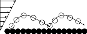
Figure 1. Sketch of a particle driven into saltation over a rigid, bumpy bed by a shearing flow.
The balance equations for the y and x-momenta of the particles, under steady and fully developed conditions, are, respectively,
 \begin{equation}\frac{{\textrm{d}{\sigma _y}}}{{\textrm{d}y}} = - c;\end{equation}
and
 \begin{equation}\frac{{\textrm{d}s}}{{\textrm{d}y}} = - c{C_D}(U - u),\end{equation}
where  ${\sigma _y}$ and s are the particle normal stress in the y-direction and the particle shear stress, respectively; c is the particle volume concentration; and CD is the drag coefficient that, for a single particle, has a component independent of the relative velocity between the single particle and the fluid and a component proportional to the absolute value of that velocity difference. Here, we assume perhaps the simplest form of CD (Dallavalle Reference Dallavalle1943), which we make independent of y by evaluating it at the bed in the case of saltation in viscous flows,
 \begin{equation}{C_D} = \frac{{18}}{{St}} + \frac{{0.3}}{r}|{U_0} - {u_0}|,\end{equation}
where St = rR is the fall Stokes number and the subscript 0 indicates quantities evaluated at the bed. We employ the terms Stokes drag to refer to situations in which  ${C_D} \simeq 18/St$, form drag for situations in which
  ${C_D} \simeq 0.3|{U_0} - {u_0}|/r$ and nonlinear drag for the generic case in which both Stokes and form drag are present. A more appropriate expression for the average CD should also involve the strength of the particle velocity fluctuations (Jenkins & Hanes Reference Jenkins and Hanes1998). However, including it would have only a small quantitative effect on the results. Also permitting the drag coefficient to vary along y does not significantly alter the solution to the continuum model. We anticipate that, while (2.3a) works well for saltation in viscous shearing flows over rigid, bumpy beds, where the fluid and particle velocity profiles are approximately linear, a more appropriate expression for saltation in turbulent flows should incorporate the difference in the concentration-weighted average velocities between the two phases, as proposed by Pähtz et al. (Reference Pähtz, Liu, Xia, Hu, He and Tholen2021)
 \begin{equation}{C_D} = \frac{{18}}{{St}} + \frac{{0.3}}{r}|\bar{U} - \bar{u}|,\end{equation}
where  $\bar{U} - \bar{u} = \int_0^h {c(U - u)\,\textrm{d}y} /\int_0^h {c\,\textrm{d}y}$, with h the depth of the saltation layer.
For flows over rigid beds, we take the no-slip boundary condition for the fluid
 \begin{equation}{U_0} = 0.\end{equation}
If saltating particles with a large value of the coefficient of sliding friction impact a rigid, bumpy bed at a small mean angle θ with respect to the horizontal (figure 1), then, using the analysis of Lämmel et al. (Reference Lämmel, Dzikowski, Kroy, Oger and Valance2017) in Appendix C,
 \begin{equation}{u_0} = {\alpha _u}\frac{1}{{{C_D}\theta }},\end{equation}
where αu is a strictly positive coefficient of order unity that is weakly dependent on the rebound properties of the particles and the flow regime of the fluid. The reason for the latter dependence is that the probability distributions of impact angles are qualitatively different for saltation in viscous and turbulent shearing flows (Appendix C).
In a steady, uniform flow, in the absence of a horizontal pressure gradient, the sum of the fluid and particle shear stress, S and s, respectively, is constant and equal to the far-field fluid shear stress, which, in dimensionless terms, is the Shields parameter
 \begin{equation}s + S = Sh.\end{equation}
To close the problem, we require constitutive relations for the particle and fluid stresses.
In the absence of particle collisions above the bed, the only mechanism responsible for the particle stresses is the transfer of momentum associated with the particles crossing a reference surface. Hence, the particle normal stress in the y-direction is simply given by the average vertical flux of y-momentum
 \begin{equation}{\sigma _y} = c{T_y},\end{equation}
where  ${T_y}$ is the mean square of the vertical velocity fluctuations of the particles . There is a corresponding mean square of the horizontal velocity fluctuations Tx, where Tx and Ty are the diagonal components of the second moment of the particle velocity tensor.
The distribution of the additional hydrodynamic field, Ty, along y is governed by the balance of kinetic energy associated with the particle vertical motion, that is, the yy-component of the particle second-moment tensor, which, in a steady and fully developed flow, and in the absence of mid-trajectory collisions and fluid velocity fluctuations, reduces to (Saha & Alam Reference Saha and Alam2016, Reference Saha and Alam2017)
 \begin{equation}{-}\frac{{\textrm{d}{Q_{yyy}}}}{{\textrm{d}y}} - 2{C_D}{\sigma _y} = 0.\end{equation}
Here,  ${Q_{yyy}}$ is the y-component of the flux of the kinetic energy associated with the vertical particle velocity fluctuations and
  $2{C_D}{\sigma _y}$ is its dissipation due to the fluid drag.
Assuming that the fluid motion is only horizontal and that the drag coefficient is independent of y, we can obtain approximate analytical expressions for the trajectories of the saltating particles even in the turbulent case (Appendix A). In doing so, we distinguish between ascending and descending particles. Then, the horizontal,  $\xi _x^ -$, and vertical,
  $\xi _y^ -$, velocities of any descending particle at a given distance y from the bed can be obtained analytically from the horizontal,
  $\xi _x^ +$, and vertical,
  $\xi _y^ +$, velocities of the same particle at the same distance y from the bed during its ascending motion. In the classical framework of statistical mechanics, we introduce a velocity distribution function,
  ${f^ + }$, for the ascending particles, so that
  $({\rm \pi}/6)\int_{all\;{\xi ^ + }} {{f^ + }\,{\textrm{d}^2}{\boldsymbol{\xi} ^ + }}$ gives the concentration of the ascending particles. With this,
  ${Q_{yyy}} = ({\rm \pi}/6)\int_{all\;{\xi ^ + }} {(\xi _y^{+2} - \xi _y^{-2}){\xi _y^{+}} {f^ + }\,{\textrm{d}^2}{\boldsymbol{\xi} ^ + }}$. With the further assumptions that the velocity distribution function is an anisotropic Maxwellian (Creyssels et al. Reference Creyssels, Dupont, Ould El Moctar, Valance, Cantat, Jenkins, Pasini and Rasmussen2009) and that the vertical velocity
  $\xi _y^ +$ of the ascending particles is much larger than 1/CD (the settling velocity), we derive a simple expression for
  ${Q_{yyy}}$ in Appendix B
 \begin{equation}{Q_{yyy}} = \sqrt {\frac{8}{\rm \pi}} {c^ + }{(T_y^ + )^{3/2}}.\end{equation}
Here, c + and  $T_y^ + $ are the volume concentration and the mean square of the vertical velocity fluctuations of the ascending particles, respectively. In a steady state, c + and
  $T_y^ + $ are related to c and Ty through (see Appendix B)
 \begin{equation}c = {c^ + }\left( {2 + \frac{3}{4}{C_D}\sqrt {\frac{{2T_y^ + }}{\rm \pi}} } \right);\end{equation}
and
 \begin{equation}{T_y} = \frac{{4\sqrt{{\rm \pi} } {C_D}T_y^{+} + 4\sqrt {2T_y^ + } }}{{8\sqrt{{\rm \pi} } {C_D} + 3C_D^2\sqrt {2T_y^ + } }}.\end{equation}
As explicitly shown in Appendix B, the assumption that the vertical velocity of the ascending particles is much larger than the settling velocity is a good approximation for  ${C_D}\sqrt {{T_y}} > 1$. We will see in § 4 that this condition is not satisfied only near the top of the saltation layer.
Using (2.7), (2.10) and (2.11) into (2.1) leads to
 \begin{equation}\frac{{\textrm{d}{c^ + }}}{{\textrm{d}y}} = - {c^ + }\frac{{8{C_D} + 3C_D^2\sqrt {2T_y^ +{/}{\rm \pi}} }}{{4{C_D}T_y^{+} + 4\sqrt {2T_y^ +{/}{\rm \pi}} }} - {c^ + }\frac{{2{C_D} + \sqrt {2/{\rm \pi} T_y^ + } }}{{2{C_D}T_y^{+} + 2\sqrt {2T_y^ +{/}{\rm \pi}} }}\frac{{\textrm{d}T_y^ + }}{{\textrm{d}y}},\end{equation}
that, combined with (2.8) and (2.9), permits an ordinary differential equation for  $T_y^ + $ to be obtained
 \begin{equation}[\sqrt {8{\rm \pi}} {C_D}{(T_y^ + )^{3/2}} + 8T_y^ + ]\frac{{\textrm{d}T_y^ + }}{{\textrm{d}y}} = (6 - 4{\rm \pi} )C_D^2{(T_y^ + )^2} - 8T_y^ + .\end{equation}
The analytical solution of this, with the boundary condition  $T_y^ + (y = 0) = T_{y,0}^ +$, for the vertical particle velocity fluctuations at the rigid boundary, is
 \begin{align}
& 4\sqrt {2{{\rm \pi} (}2{\rm \pi} - 3\textrm{)}} {\tan ^{ - 1}}\left( {\dfrac{{\sqrt {2{\rm \pi} - 3} }}{2}{C_D}\sqrt {T_y^ + } } \right)\nonumber\\
& \qquad - 2(2{\rm \pi} - 3)\left\{ {\sqrt {2{\rm \pi}} {C_D}\sqrt {T_y^ + } + 2\log [4 + (2{\rm \pi} - 3)C_D^2T_y^ + ]} \right\}\nonumber\\
& \quad = {(3 - 2{\rm \pi} )^2}C_D^2y + 4\sqrt {2{{\rm \pi} (}2{\rm \pi} - 3\textrm{)}} {\tan ^{ - 1}}\left( {\dfrac{{\sqrt {2{\rm \pi} - 3} }}{2}{C_D}\sqrt {T_{y,0}^ + } } \right)\nonumber\\
& \qquad - 2(2{\rm \pi} - 3)\left\{ {\sqrt {2{\rm \pi}} {C_D}\sqrt {T_{y,0}^ + } + 2\log [4 + (2{\rm \pi} - 3)C_D^2T_{y,0}^ + ]} \right\}.
\end{align}
\begin{align}
& 4\sqrt {2{{\rm \pi} (}2{\rm \pi} - 3\textrm{)}} {\tan ^{ - 1}}\left( {\dfrac{{\sqrt {2{\rm \pi} - 3} }}{2}{C_D}\sqrt {T_y^ + } } \right)\nonumber\\
& \qquad - 2(2{\rm \pi} - 3)\left\{ {\sqrt {2{\rm \pi}} {C_D}\sqrt {T_y^ + } + 2\log [4 + (2{\rm \pi} - 3)C_D^2T_y^ + ]} \right\}\nonumber\\
& \quad = {(3 - 2{\rm \pi} )^2}C_D^2y + 4\sqrt {2{{\rm \pi} (}2{\rm \pi} - 3\textrm{)}} {\tan ^{ - 1}}\left( {\dfrac{{\sqrt {2{\rm \pi} - 3} }}{2}{C_D}\sqrt {T_{y,0}^ + } } \right)\nonumber\\
& \qquad - 2(2{\rm \pi} - 3)\left\{ {\sqrt {2{\rm \pi}} {C_D}\sqrt {T_{y,0}^ + } + 2\log [4 + (2{\rm \pi} - 3)C_D^2T_{y,0}^ + ]} \right\}.
\end{align}
The non-zero value of  $T_{y,0}^ +$ is associated with the rebound velocity of the particles at a rigid, bumpy bed.
Under the same assumptions that were employed to derive equation (2.5), a simple dependence of  $T_{y,0}^ +$ calculated at the bed on the impact angle θ is obtained in Appendix C
 \begin{equation}T_{y,0}^ + = {\alpha _T}\frac{1}{{C_D^2\theta }}\frac{{2{d_w}}}{{1 + {d_w}}},\end{equation}
where αT is another strictly positive coefficient of order unity that is weakly dependent on the rebound properties of the particles and the flow regime of the fluid. We emphasize that the impact angle, and consequently  $T_{y,0}^ +$, remains an unknown at this stage of the analysis. We will determine it in the next two sub-sections, when we describe quantities associated with the horizontal motion of the particles that are influenced by the flow regime of the fluid.
Equation (2.14) provides the analytical distribution of  $T_y^ +$ along y, which, when employed in (2.11), gives the analytical distribution of Ty shown in figure 2(a) for different values of
  ${C_D}\sqrt {T_{y,0}^ + }$, corresponding to an impact angle θ in (2.15) in the range 1° to 20°. As shown in figure 2(b), the distribution of Ty is roughly linear and well approximated as
 \begin{equation}{T_y} = \frac{{h - y}}{h}{T_{y,0}},\end{equation}
where the depth of the saltation layer, h, is to be determined. The mean square of the particle velocity fluctuations at the bed,  ${T_{y,0}}$, can be obtained from (2.11), when
  $T_{y,0}^ +$ is known.

Figure 2. (a) Normalized profiles of  $T_y^ + $ (dot-dashed lines) and Ty (dashed lines) obtained from (2.14) and (2.11), respectively, when
  $C_D^2T_{y,0}^ + = 2.5$ (blue lines),
  $C_D^2T_{y,0}^ + = 10$ (orange lines) and
  $C_D^2T_{y,0}^ + = 100$ (purple lines). (b) Normalized profiles of Ty (dashed lines, same colour legend of figure 2a) and the linear distribution of (2.16) (solid black line).
Inserting (2.7) into (2.1), with (2.16), and integrating gives the following power-law distribution of the particle concentration:
 \begin{equation}c = {c_0}{\left( {\frac{{h - y}}{h}} \right)^{(h - {T_{y,0}})/{T_{y,0}}}},\end{equation}
where c 0 is the particle concentration at the bed. Integrating equation (2.1) with (2.17) also gives
 \begin{equation}{\sigma _y} = {c_0}{T_{y,0}}{\left( {\frac{{h - y}}{h}} \right)^{h/{T_{y,0}}}}.\end{equation}
Upon introducing the hold-up,  $M = \int_0^h {c\,\textrm{d}y}$, i.e. the particle mass per unit basal area, by integrating the concentration through the saltation layer, with σy = 0 at y = h, we obtain
 \begin{equation}{c_0} = \frac{M}{{{T_{y,0}}}}.\end{equation}
Integrating the energy balance, (2.8) with (2.18) and (2.19), provides
 \begin{equation}{Q_{yyy}} = 2{C_D}M{T_{y,0}}\frac{h}{{h + {T_{y,0}}}}\left[ {{{\left( {\frac{{h - y}}{h}} \right)}^{(h + {T_{y,0}})/{T_{y,0}}}} - 1} \right] + {Q_{yyy,0}},\end{equation}
where the value of Qyyy at the bed can be obtained from the ratio of (2.9) and (2.7), with (2.10), (2.11) and (2.19), as
 \begin{equation}{Q_{yyy,0}} = \frac{{4{C_D}T_{y,0}^ + }}{{{C_D}\sqrt {2{\rm \pi} T_{y,0}^ + } + 2}}M.\end{equation}
Given that Qyyy must vanish at the top of the saltation layer, the depth h of the saltation layer is determined from (2.20) as
 \begin{equation}h = \frac{{{Q_{yyy,0}}}}{{2{C_D}M{T_{y,0}} - {Q_{yyy,0}}}}{T_{y,0}}.\end{equation}
The governing equations, constitutive relations and analytical results described so far apply to saltation in both viscous and in turbulent shearing flows and can be calculated only after the determination of the impact angle θ, required in (2.5) and (2.15). To proceed, we must distinguish between the two regimes of the fluid shearing flow.
Before doing that, we support the assumption that particle collisions above the bed can be neglected. As suggested by Pasini & Jenkins (Reference Pasini and Jenkins2005), chances of mid-trajectory collisions are low if the mean free path, λ, the average distance travelled by a particle in between two successive collisions predicted by the kinetic theory of granular gases, is less than twice the height of the particle trajectory, here determined by gravity and fluid drag. If we use the expression for the mean free path in a dilute gas of Chapman & Cowling (Reference Chapman and Cowling1970), evaluate this at the bed and take h as the average height of the particle trajectories, we obtain
 \begin{equation}{\lambda _0} = \frac{1}{{6{c_0}\sqrt 2 }} \ge 2h.\end{equation}
Equation (2.23), used with (2.22), implies that, for given values of r, St and Sh, there is a maximum hold-up above which mid-trajectory collisions play a role. That is, because the mean free path is a decreasing function of the particle concentration, as the hold-up increases, collisions become more likely. However, there is also a limiting hold-up at which particles begin to deposit on the bed. Analysis of periodic trajectories over rigid beds (Jenkins & Valance Reference Jenkins and Valance2014) and discrete simulations of the present paper indicate that the concentration at the bed at which deposition begins is greater than that at which collisions begin to occur. Consequently, in saltation over such beds, collisions occur before deposition.
2.1. Saltation in viscous shearing flows
In the absence of turbulence, the expression for the fluid shear stress is (Valance & Berzi Reference Valance and Berzi2022)
 \begin{equation}S = \frac{{1 - c}}{{St}}\frac{{\textrm{d}U}}{{\textrm{d}y}} \simeq \frac{1}{{St}}\frac{{\textrm{d}U}}{{\textrm{d}y}},\end{equation}
where we have neglected the particle concentration with respect to unity. Equation (2.24) implies that, in the absence of particles and in the boundary layer approximation that we have employed, the fluid velocity distribution would be linear.
Using statistical mechanics arguments, the particle shear stress can be obtained as  $s = - ({\rm \pi}/6)\int_{all\;{\xi ^ + }} {({\xi _x^{+}} - {\xi _x^{-}} ){\xi _y^{+}} {f^ + }\,{\textrm{d}^2}{\boldsymbol{\xi} ^ + }}$. To determine
  $\xi _x^ -$, we assume in Appendix A that the fluid velocity profile encountered by an ascending particle during its ballistic trajectory above a certain position y is locally linear; that is, it is linear in the region between y and the top of the trajectory. However, the slope of the linear profile changes with y due to the drag of the particles. This assumption and the assumptions on the form of the velocity distribution function
  ${f^ + }$ and
  ${C_D}\xi _y^ + \gg 1$, that we have already employed in the derivation of the expression for Qyyy in (2.9), permit the derivation in Appendix B of a simple expression for the particle shear stress
 \begin{equation}s = \frac{3}{5}{C_D}{\sigma _y}\left( {U - u + \frac{2}{3}\frac{1}{{C_D^2}}\frac{{\textrm{d}U}}{{\textrm{d}y}}} \right).\end{equation}
Interestingly, the particle shear stress does not depend on the particle shear rate, as in Jenkins et al. (Reference Jenkins, Cantat and Valance2010), but only on the velocity difference and on the fluid shear rate. The physical reason is that the particles do not interact with each other, but only with the surrounding fluid.
As explained in Appendix C, for saltation in viscous flows the mean angle θ between the particle velocity and the horizontal before the impact with the bed is estimated in the limit of large vertical velocity of ascending particles in Appendix A as
 \begin{equation}\theta = \frac{{{C_D}}}{{St(Sh - {s_0})}},\end{equation}
where s 0 is the particle shear stress at the bed.
Using (2.4) and (2.5) in (2.3a), with (2.26), we obtain a relationship between the drag coefficient and the particle shear stress at the bed
 \begin{equation}C_D^3 = \frac{{18}}{{St}}C_D^2 + \frac{{0.3}}{r}{\alpha _u}St(Sh - {s_0}).\end{equation}
The particle shear stress at the bed is obtained from (2.25), with (2.4)–(2.6), (2.19) and (2.24), as
 \begin{equation}{s_0} = \frac{{(2 - 3{\alpha _u})MStSh}}{{5{C_D} + (2 - 3{\alpha _u})MSt}}.\end{equation}
Equation (2.28) implies that for the particle shear stress at the bed to be positive, αu must be less than 2/3. The system of (2.27) and (2.28) can be solved to determine the drag coefficient and the particle shear stress at the bed once the values of dw, r, St, Sh and M are given. Then, the impact angle (2.26), the values of all the variables at the bed ((2.5), (2.15) and (2.21)), the depth of the saltation layer (2.22), and the analytical distributions of  $T_y^ + $, Ty, c, σy and Qyyy ((2.14), (2.16)–(2.18) and (2.20)) can also be calculated for saltation in viscous shearing flows.
Figure 3 shows the variation of the impact angle, the drag coefficient and the particle shear stress at the bed with the particle hold-up, as predicted by ((2.26)–(2.28)), for, e.g. saltation of 100  ${\rm \mu}$m basalt grains in viscous shearing flows on Venus, assuming that αu = 0.60 (§ 4 provides more details on the choice of the parameters). Equation (2.23) is satisfied for the range of hold-up in figure 3. Notice that for almost the entire range of hold-up, the particle shear stress at the bed increases linearly with M, while θ and CD are constant.

Figure 3. Predicted impact angle in degrees (solid line, –), drag coefficient (dashed line, ‐‐) and particle shear stress at the bed (dot-dashed line, ⋅-) as functions of the hold-up for saltation in viscous shearing flows when dw = 1, St = 100, r = 50, and Sh = 0.05 (with αu = 0.60).
Using (2.25) in (2.2), with (2.6), (2.18) and (2.24), gives a first-order, linear, non-homogeneous, differential equation for the particle shear stress
 \begin{align}\frac{{\textrm{d}s}}{{\textrm{d}y}} = - \left[ {\frac{5}{3}\frac{1}{{{T_{y,0}}}}{{\left( {\frac{{h - y}}{h}} \right)}^{ - 1}} + \frac{2}{3}\frac{{{c_0}St}}{{{C_D}}}{{\left( {\frac{{h - y}}{h}} \right)}^{(h - {T_{y,0}})/{T_{y,0}}}}} \right]s + \frac{2}{3}\frac{{{c_0}StSh}}{{{C_D}}}{\left( {\frac{{h - y}}{h}} \right)^{(h - {T_{y,0}})/{T_{y,0}}}}.\end{align}
The analytical solution of (2.29) is
 \begin{align}
s & = Sh{\left({\dfrac{2}{3}\dfrac{{MSt}}{{{C_D}}}} \right)^{5/3}}\varGamma \left[ { -
\dfrac{2}{3},\dfrac{2}{3}\dfrac{{MSt}}{{{C_D}}}{{\left( {\dfrac{{h - y}}{h}} \right)}^{h/{T_{y,0}}}}}
\right]\nonumber\\
&\quad \times \exp \left\{ {\ln \left[ {{{\left( {\dfrac{{h - y}}{h}} \right)}^{(5/3)(h/{T_{y,0}})}}} \right] +
\dfrac{2}{3}\dfrac{{MSt}}{{{C_D}}}{{\left( {\dfrac{{h - y}}{h}} \right)}^{h/{T_{y,0}}}}} \right\}\nonumber\\
& \quad - Sh{\left( {\dfrac{2}{3}\dfrac{{MSt}}{{{C_D}}}} \right)^{5/3}}\varGamma \left[ { -
\dfrac{2}{3},\dfrac{2}{3}\dfrac{{MSt}}{{{C_D}}}} \right]\nonumber\\
&\quad \times \exp \left\{ {\ln \left[ {{{\left( {\dfrac{{h -
y}}{h}} \right)}^{(5/3)(h/{T_{y,0}})}}} \right] + \dfrac{2}{3}\dfrac{{MSt}}{{{C_D}}}{{\left( {\dfrac{{h -
y}}{h}} \right)}^{h/{T_{y,0}}}}} \right\}\nonumber\\
& \quad + {s_0} \exp \left\{ {\ln \left[ {{{\left( {\dfrac{{h -
y}}{h}} \right)}^{(5/3)(h/{T_{y,0}})}}} \right] + \dfrac{2}{3}\dfrac{{MSt}}{{{C_D}}}{{\left( {\dfrac{{h -
y}}{h}} \right)}^{h/{T_{y,0}}}} - \dfrac{2}{3}\dfrac{{MSt}}{{{C_D}}}} \right\},
\end{align}
\begin{align}
s & = Sh{\left({\dfrac{2}{3}\dfrac{{MSt}}{{{C_D}}}} \right)^{5/3}}\varGamma \left[ { -
\dfrac{2}{3},\dfrac{2}{3}\dfrac{{MSt}}{{{C_D}}}{{\left( {\dfrac{{h - y}}{h}} \right)}^{h/{T_{y,0}}}}}
\right]\nonumber\\
&\quad \times \exp \left\{ {\ln \left[ {{{\left( {\dfrac{{h - y}}{h}} \right)}^{(5/3)(h/{T_{y,0}})}}} \right] +
\dfrac{2}{3}\dfrac{{MSt}}{{{C_D}}}{{\left( {\dfrac{{h - y}}{h}} \right)}^{h/{T_{y,0}}}}} \right\}\nonumber\\
& \quad - Sh{\left( {\dfrac{2}{3}\dfrac{{MSt}}{{{C_D}}}} \right)^{5/3}}\varGamma \left[ { -
\dfrac{2}{3},\dfrac{2}{3}\dfrac{{MSt}}{{{C_D}}}} \right]\nonumber\\
&\quad \times \exp \left\{ {\ln \left[ {{{\left( {\dfrac{{h -
y}}{h}} \right)}^{(5/3)(h/{T_{y,0}})}}} \right] + \dfrac{2}{3}\dfrac{{MSt}}{{{C_D}}}{{\left( {\dfrac{{h -
y}}{h}} \right)}^{h/{T_{y,0}}}}} \right\}\nonumber\\
& \quad + {s_0} \exp \left\{ {\ln \left[ {{{\left( {\dfrac{{h -
y}}{h}} \right)}^{(5/3)(h/{T_{y,0}})}}} \right] + \dfrac{2}{3}\dfrac{{MSt}}{{{C_D}}}{{\left( {\dfrac{{h -
y}}{h}} \right)}^{h/{T_{y,0}}}} - \dfrac{2}{3}\dfrac{{MSt}}{{{C_D}}}} \right\},
\end{align}
in which  $\varGamma (s,x) \equiv \int_x^\infty {{t^{s - 1}}\,{e^{ - t}}\,{\rm d}t}$ is the upper incomplete gamma function.
The fluid velocity profile is determined by integrating the constitutive relation (2.24)  $\textrm{d}U/\textrm{d}y = St(Sh - s)$, with the particle shear stress given by (2.30). Unfortunately, there is no general analytical solution. Hence, we obtain the distribution of U by numerically solving this ordinary differential equation, with the no-slip condition, (2.4), at the bed. Once U is determined, the particle horizontal velocity is given by (2.25) as
 \begin{equation}u = U - \frac{5}{3}\frac{s}{{{C_D}{\sigma _y}}} + \frac{2}{3}\frac{{St(Sh - s)}}{{C_D^2}}.\end{equation}
We can now calculate the particle flux q per unit basal area through numerical integration as
 \begin{equation}q = \int_0^h {cu\,\textrm{d}y} .\end{equation}
 In the special case of rarefied saltation, that is for  $M \to 0$ and
  $Sh \gg s$, the analytical solution of (2.29) simplifies to
 \begin{equation}s = {s_0}{\left( {\frac{{h - y}}{h}} \right)^{(5/3)(h/{T_{y,0}})}} + \frac{{MStSh}}{{{C_D}}}\left[ {{{\left( {\frac{{h - y}}{h}} \right)}^{h/{T_{y,0}}}} - {{\left( {\frac{{h - y}}{h}} \right)}^{(5/3)(h/{T_{y,0}})}}} \right],\end{equation}
and the fluid velocity profile is simply
 \begin{equation}U = (StSh)y.\end{equation}
Then, from (2.18), (2.28), (2.31), (2.33) and (2.34), the particle horizontal velocity is
 \begin{equation}u = \left[ {(1 + {\alpha_u}){{\left( {\frac{{h - y}}{h}} \right)}^{(2/3)(h/{T_{y,0}})}} + C_D^2y - 1} \right]\frac{{StSh}}{{C_D^2}}.\end{equation}
Notice that, in the rarefied limit of saltation in viscous shearing flows, the particle and the fluid velocity profiles are independent of the hold-up. Using (2.17), (2.19) and (2.35) in (2.32), and integrating, gives the particle flux as
 \begin{equation}q = MStSh{T_{y,0}}\frac{h}{{h + {T_{y,0}}}}.\end{equation}
The above equations permit the determination of profiles of particle concentration, particle and fluid velocities and particle and fluid stresses in viscous shearing flow that will be compared with the results of DC numerical simulations in § 4.
2.2. Saltation in turbulent shearing flows
In the case of saltation in turbulent shearing flows, we model the fluid shear stress using the classical mixing length approach (Jenkins et al. Reference Jenkins, Cantat and Valance2010)
 \begin{equation}S = \frac{{1 - c}}{r}{\kappa ^2}{(y + {y_0})^2}{\left( {\frac{{\textrm{d}U}}{{\textrm{d}y}}} \right)^2} \simeq \frac{{{\kappa ^2}{{(y + {y_0})}^2}}}{r}{\left( {\frac{{\textrm{d}U}}{{\textrm{d}y}}} \right)^2},\end{equation}
where κ = 0.41 is von Kármán's constant and  ${y_0} = \sqrt {r/Sh} /(9St) + ({k_s}/30)[1 - \exp ( - {k_s}St\sqrt {Sh/r} /26)]$ is an empirical expression for the origin of the logarithmic fluid velocity profile that encompasses hydrodynamically smooth, rough and transitional beds (Guo & Julien Reference Guo and Julien2007). The roughness length scale ks is taken to be equal to dw (Ho Reference Ho2012).
Equation (2.37) implies that, in the absence of particles and in the boundary layer approximation that we have employed, the fluid velocity distribution would be logarithmic. We assume, as in Pähtz et al. (Reference Pähtz, Liu, Xia, Hu, He and Tholen2021), that the fluid velocity profile encountered by an ascending particle during its ballistic trajectory is logarithmic even if other particles are present. This assumption, and the assumptions that we have already employed in the derivation of the expression for Qyyy, (2.9), permits the derivation in Appendix B of an expression for the particle shear stress,  $s = - ({\rm \pi}/6)\int_{all\;{\xi ^ + }} {(\xi _x^ + - \xi _x^ - )\xi _y^ + {f^ + }\,{\textrm{d}^2}{\xi ^ + }}$
 \begin{align} s &=
\frac{3}{5}{C_D}{\sigma _y}\left\{ {U - u - \frac{{\sqrt
{rS} }}{\kappa }\exp \left[ {{C_D^2}\frac{{\sqrt {rS}
}}{\kappa }{{\left( {\frac{{\textrm{d}U}}{{\textrm{d}y}}}
\right)}^{ - 1}}} \right]Ei\left[ { - {C_D^2}\frac{{\sqrt
{rS} }}{\kappa }{{\left(
{\frac{{\textrm{d}U}}{{\textrm{d}y}}} \right)}^{ - 1}}}
\right]}
\right\},\end{align}
\begin{align} s &=
\frac{3}{5}{C_D}{\sigma _y}\left\{ {U - u - \frac{{\sqrt
{rS} }}{\kappa }\exp \left[ {{C_D^2}\frac{{\sqrt {rS}
}}{\kappa }{{\left( {\frac{{\textrm{d}U}}{{\textrm{d}y}}}
\right)}^{ - 1}}} \right]Ei\left[ { - {C_D^2}\frac{{\sqrt
{rS} }}{\kappa }{{\left(
{\frac{{\textrm{d}U}}{{\textrm{d}y}}} \right)}^{ - 1}}}
\right]}
\right\},\end{align}
in which  $Ei(x) \equiv{-} \int_{ - x}^\infty {{e^{ - t}}{t^{ - 1}}\,{\rm d}t} $ is the exponential integral. As in the viscous case of (2.25), the particle shear stress in turbulent shearing flows does not depend on the particle shear rate. The saltating particles, when treated as a continuous medium, can experience shear stress even if the horizontal particle velocity is uniform across the flow domain.
As explained in Appendix C, the mean impact angle θ for saltation in turbulent flows in the limit of large vertical velocity of ascending particles is estimated as
 \begin{equation}\theta \simeq{-} {\left[ {{C_D}\frac{{\sqrt {r(Sh - {s_0})} }}{\kappa }\exp (C_D^2{y_0})Ei( - C_D^2{y_0})} \right]^{ - 1}}.\end{equation}
Integrating equation (2.2) between y = 0 and y = h, with vanishing particle shear stress at the top of the saltation layer gives  ${s_0} = M{C_D}(\bar{U} - \bar{u})$ (Pähtz et al. Reference Pähtz, Liu, Xia, Hu, He and Tholen2021). Using this in (2.3b) gives the drag coefficient in terms of the particle shear stress at the bed
 \begin{equation}{C_D} = \frac{9}{{St}} + \sqrt {\frac{{81}}{{S{t^2}}} + \frac{{0.3}}{r}\frac{{{s_0}}}{M}} .\end{equation}
Equation (2.38) evaluated at the bed, with (2.5) and (2.39) gives the particle shear stress at the bed as a function of the impact angle
 \begin{equation}{s_0} = \frac{3}{5}\frac{M}{\theta }(1 - {\alpha _u}).\end{equation}
Equation (2.41) implies that, for the particle shear stress at the bed to be positive, αu must be less than 1. Then, (2.39) with (2.40) and (2.41) results in an implicit equation for θ
 \begin{align}
\dfrac{1}{\theta }{\left({\dfrac{9}{{St}} + \sqrt {\dfrac{{81}}{{S{t^2}}} + \dfrac{{0.9}}{{5r}}\dfrac{{1 - {\alpha_u}}}{\theta }} } \right)^{ - 1}} & \simeq{-} \dfrac{1}{\kappa }\sqrt {r\left( {Sh - \dfrac{{3M}}{5}\dfrac{{1 - {\alpha_u}}}{\theta }} \right)}\nonumber\\
&\quad \times \exp \left[ {{{\left( {\dfrac{9}{{St}} + \sqrt {\dfrac{{81}}{{S{t^2}}} + \dfrac{{0.9}}{{5r}}\dfrac{{1 - {\alpha_u}}}{\theta }} } \right)}^2}{y_0}} \right]\nonumber\\
& \quad \times Ei\left[ { - {{\left( {\dfrac{9}{{St}} + \sqrt {\dfrac{{81}}{{S{t^2}}} + \dfrac{{0.9}}{{5r}}\dfrac{{1 -
{\alpha_u}}}{\theta }} } \right)}^2}{y_0}} \right].\end{align}
\begin{align}
\dfrac{1}{\theta }{\left({\dfrac{9}{{St}} + \sqrt {\dfrac{{81}}{{S{t^2}}} + \dfrac{{0.9}}{{5r}}\dfrac{{1 - {\alpha_u}}}{\theta }} } \right)^{ - 1}} & \simeq{-} \dfrac{1}{\kappa }\sqrt {r\left( {Sh - \dfrac{{3M}}{5}\dfrac{{1 - {\alpha_u}}}{\theta }} \right)}\nonumber\\
&\quad \times \exp \left[ {{{\left( {\dfrac{9}{{St}} + \sqrt {\dfrac{{81}}{{S{t^2}}} + \dfrac{{0.9}}{{5r}}\dfrac{{1 - {\alpha_u}}}{\theta }} } \right)}^2}{y_0}} \right]\nonumber\\
& \quad \times Ei\left[ { - {{\left( {\dfrac{9}{{St}} + \sqrt {\dfrac{{81}}{{S{t^2}}} + \dfrac{{0.9}}{{5r}}\dfrac{{1 -
{\alpha_u}}}{\theta }} } \right)}^2}{y_0}} \right].\end{align}
This can be solved to determine the impact angle. Once θ is known, s 0 (2.41), CD (2.40), the boundary values of the remaining variables at the bed ((2.5), (2.15) and (2.21)), the depth of the saltation layer (2.22), and the analytical distributions of  $T_y^ + $, Ty, c, σy and Qyyy ((2.14), (2.16)–(2.18) and (2.20)) can also be calculated in saltation in turbulent shearing flows.
Figure 4 shows the variation of the impact angle, the drag coefficient and the particle shear stress at the bed with the particle hold-up, as predicted by ((2.40)–(2.42)), for saltation of 240  ${\rm \mu}$m sand grains in a turbulent wind on Earth, with αu = 0.85 (see § 4 for more details about the choice of the parameters). The range of the hold-ups in figure 4 is that for which (2.23) is satisfied. As for saltation in viscous shearing flows (figure 3), the particle shear stress at the bed increases linearly with M, while θ and CD are almost constant.
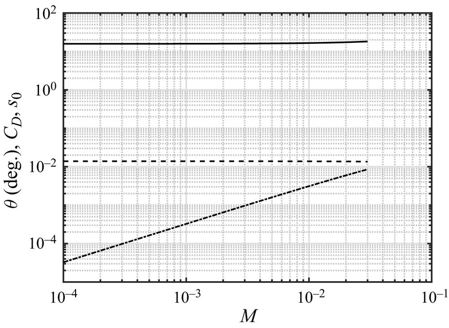
Figure 4. Predicted impact angle in degrees (solid line, –), drag coefficient (dashed line, ‐‐) and particle shear stress at the bed (dot-dashed line, ⋅-) as functions of the hold-up for saltation in turbulent shearing flows with dw = 1.5, St = 1681, r = 2208 and Sh = 0.04 (with αu = 0.85).
Equation (2.2), with (2.38) and (2.6), and (2.37) can be written as a system of two ordinary differential equations
 \begin{equation}\frac{{\textrm{d}s}}{{\textrm{d}y}} = - {C_D}c\frac{{\sqrt {r(Sh - s)} }}{\kappa }\exp [C_D^2(y + {y_0})]Ei[ - C_D^2(y + {y_0})] - \frac{5}{3}\frac{s}{{{T_y}}};\end{equation}
and
 \begin{equation}\frac{{\textrm{d}U}}{{\textrm{d}y}} = \frac{{\sqrt {r(Sh - s)} }}{{\kappa (y + {y_0})}};\end{equation}
these can be numerically integrated, with the boundary conditions of (2.4) and (2.41), to obtain the distributions of the particle shear stress and the fluid horizontal velocity. Then, the particle horizontal velocity is given by (2.38), with (2.6), as
 \begin{equation}u = U - \frac{{\sqrt {r(Sh - s)} }}{\kappa }\exp [C_D^2(y + {y_0})]Ei[ - C_D^2(y + {y_0})] - \frac{5}{3}\frac{s}{{{C_D}{\sigma _y}}}.\end{equation}
Finally, the particle flux q per unit basal area is determined through numerical integration of (2.32), with the profiles of u and c obtained under turbulent conditions.
The above equations permit the determination of profiles of particle concentration, particle and fluid velocities and particle and fluid stresses in turbulent shearing flow that will be compared with the results of DC numerical simulations in § 4.
3. Scaling laws for rarefied saltation
The semi-analytical solutions to particle saltation in shearing flows described in the previous section permit simple asymptotic scalings to be obtained in the limit of rarefied saltation,  $M \to 0$ and
  ${s_0} \ll Sh$, and: (i) only Stokes drag,
  ${C_D} = 18/St$, that is when the particle Reynolds number based upon the relative velocity between the particles and the fluid at the bed,
  ${u_0}St/r$, is less than unity; or (ii) only form drag,
  ${C_D} = 0.3{u_0}/r$, that is when
  ${10^3} < {u_0}St/r < {10^5}$. In the following, we will consider that at leading order, (2.11) and (2.22) imply that
 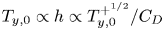 ${T_{y,0}} \propto h \propto T_{y,0}^{{ + ^{1/2}}}/{C_D}$.
We emphasize that there is no feedback of the particles on the fluid velocity profile, which, in rarefied saltation, is exactly linear in the viscous case, and logarithmic in the turbulent case. As a consequence, the particle hold-up only affects the particle concentration, is linearly proportional to it, and does not influence the particle velocity. Given that the mass flux involves the product of particle concentration and horizontal velocity, q must also be linearly related to the hold-up.
3.1. Rarefied saltation in viscous shearing flows with Stokes drag
In this case, the density ratio plays no role in the equations governing the saltation process. As mentioned,  ${C_D} \propto S{t^{ - 1}}$. Then, with (2.26), we obtain that
 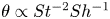 $\theta \propto S{t^{ - 2}}S{h^{ - 1}}$. With this, (2.5), (2.15), (2.19) and (2.36) imply the scalings for the various quantities that we report in table 1. In particular, we note that the scaling for the particle flux,
 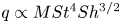 $q \propto MS{t^4}S{h^{3/2}}$, was also derived in Valance & Berzi (Reference Valance and Berzi2022) using an approach in which all particles were assumed to follow the same PT, and not a distribution of trajectories as in the present work.
Table 1. Summary of the scaling laws for rarefied saltation.
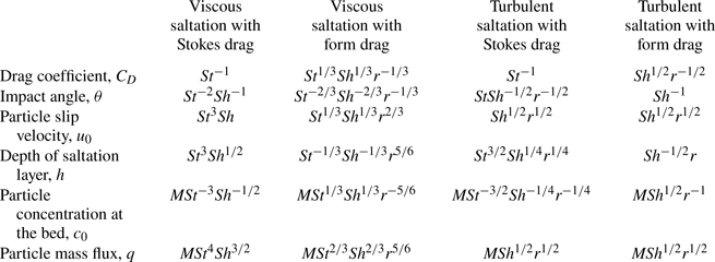
3.2. Rarefied saltation in viscous shearing flows with form drag
In the case of form drag,  ${C_D} \propto {u_0}{r^{ - 1}}$, and we expect the scaling laws to involve also the density ratio. With (2.5), we obtain
 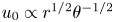 ${u_0} \propto {r^{1/2}}{\theta ^{ - 1/2}}$, and, with (2.26) and (2.15),
 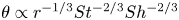 $\theta \propto {r^{ - 1/3}}S{t^{ - 2/3}}S{h^{ - 2/3}}$ and
  $T_{y,0}^ +\propto r$. Hence, (2.5), (2.15), (2.19) and (2.36) imply the scalings for the various quantities that we report in table 1.
3.3. Rarefied saltation in turbulent shearing flows with Stokes drag
In this case,  ${C_D} \propto S{t^{ - 1}}$. At leading order, (2.39) gives
  $\theta \propto C_D^{ - 1}{r^{ - 1/2}}S{h^{ - 1/2}} \propto {r^{ - 1/2}}StS{h^{ - 1/2}}$ and (2.15) gives
 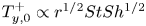 $T_{y,0}^ +\propto {r^{1/2}}StS{h^{1/2}}$. With (2.5), we obtain
 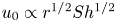 ${u_0} \propto {r^{1/2}}S{h^{1/2}}$, and from (2.21) and (2.22),
 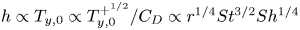 $h \propto {T_{y,0}} \propto T_{y,0}^{{ + ^{1/2}}}/{C_D} \propto {r^{1/4}}S{t^{3/2}}S{h^{1/4}}$. Equation (2.19), then, provides
  ${c_0} \propto M{r^{ - 1/4}}S{t^{ - 3/2}}S{h^{ - 1/4}}$. As shown later, the concentration and particle velocity profiles in the case of turbulent saltation are approximately uniform across the flow. Therefore, we expect
 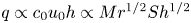 $q \propto {c_0}{u_0}h \propto M{r^{1/2}}S{h^{1/2}}$. See the summary of the scalings in table 1.
3.4. Rarefied saltation in turbulent shearing flows with form drag
In this limiting case, the fall Stokes number, St, plays no role in the equations governing saltation and cannot be involved in the scalings. With 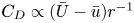 ${C_D} \propto (\bar{U} - \bar{u}){r^{ - 1}}$ and
 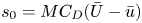 ${s_0} = M{C_D}(\bar{U} - \bar{u})$ with (2.41), we obtain
 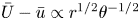 $\bar{U} - \bar{u} \propto {r^{1/2}}{\theta ^{ - 1/2}}$, and, with (2.39) and (2.15), at leading order,
 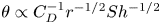 $\theta \propto C_D^{ - 1}{r^{ - 1/2}}S{h^{ - 1/2}}$ and
 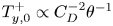 $T_{y,0}^ +\propto C_D^{ - 2}{\theta ^{ - 1}}$. Hence,
  $\theta \propto S{h^{ - 1}}$,
  $T_{y,0}^ +\propto r$,
  ${u_0} \propto {r^{1/2}}S{h^{1/2}}$,
  ${C_D} \propto {r^{ - 1/2}}S{h^{1/2}}$ and
 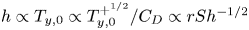 $h \propto {T_{y,0}} \propto T_{y,0}^{{ + ^{1/2}}}/{C_D} \propto rS{h^{ - 1/2}}$. Equation (2.19), then, provides
  ${c_0} \propto M{r^{ - 1}}S{h^{1/2}}$. As mentioned, the concentration and particle velocity profiles in the case of turbulent saltation are approximately uniform across the flow. Therefore, we expect
  $q \propto {c_0}{u_0}h \propto MS{h^{1/2}}{r^{1/2}}$. We incorporate the scaling laws for rarefied turbulent saltation with form drag in table 1.
4. Comparisons with numerical simulations and experiments
Here, we make comparisons between the predictions of the present theory and the results of DC numerical simulations of saltation of spheres over a rigid bumpy bed made of a layer of particles in close contact. The simulations are performed in a quasi-two-dimensional cell of streamwise length equal to 5120 particle diameters and transverse width equal to one particle diameter, with periodic boundary conditions in the streamwise direction. The cell is not bounded above. We checked that increasing the length in the streamwise direction up to ten times had no effect on the results. Data are available at https://doi.org/10.5281/zenodo.11264272 (Valance Reference Valance2024).
We solve Newton's equations of motion for the individual spherical particles under the influence of fluid drag, buoyancy, gravity and contact forces in collisions with the bed. Mid-trajectory collisions are forbidden. The fluid is treated as either a viscous or a turbulent flow, depending on the closure for the fluid shear stress, which is governed by a balance equation. The sum over all particles of drag and buoyancy enters the momentum balance for the fluid with a change in sign, thus ensuring the two-way coupling between the phases. In the numerical simulations, we assume that the fluid possesses only horizontal velocity and suppress the possibility of interparticle collisions above the bed.
The individual particles experience vertical and horizontal components of fluid drag based upon the local difference between the instantaneous velocity of the particle and the average velocity of the fluid. As in the theoretical treatment, we control the amount of particles in the simulations (the particle hold-up, M); the bumpiness of the rigid bed (the wall-particle diameter, dw); the fluid viscosity (the inverse of the fall Stokes number, St); the fluid mass density (the inverse of the density ratio, r); and the intensity of the shearing flow (the Shields number, Sh). All measurements have been taken once a steady state is attained and, subsequently, time averaged. Such numerical simulations have already been used in the context of saltation in both turbulent (Durán et al. Reference Durán, Andreotti and Claudin2012; Pähtz et al. Reference Pähtz, Durán, Ho, Valance and Kok2015; Pähtz & Durán Reference Pähtz and Durán2020; Ralaiarisoa et al. Reference Ralaiarisoa, Besnard, Furieri, Dupont, Ould El Moctar, Naaim-Bouvet and Valance2020) and viscous (Valance & Berzi Reference Valance and Berzi2022) shearing flows. A more detailed description of the numerical simulations, including the contact parameters that we employ, can be found in Appendix D.
In a total of 50 simulations, we have numerically investigated the saltation process of four different types of solid particles in terrestrial and extra-terrestrial environment, as summarized in table 2, by changing the particle hold-up between 0.0004 and approximately 0.0300, that is, from the rarefied limit to the maximum hold-up for which the mid-trajectory collisions can be neglected and (2.23) is satisfied. Although the fluid regime on Mars and Venus is almost certainly turbulent, one can at least imagine performing experiments in pressurized wind tunnels, in which the turbulence is somehow suppressed, thus recovering the conditions reported in the first two rows of table 2. The conditions reported in the last two rows of table 2 are, instead, much closer to actual physical applications.
Table 2. Summary of the combination of parameters employed in the numerical simulations.

The flow conditions chosen serve to isolate and test the assumptions that we have made in building the theory: (i) an anisotropic Maxwellian velocity distribution for the particles, the vertical velocity of the ascending particles much larger than the settling velocity and a locally linear velocity for the fluid in the viscous regime, with Stokes drag (the first row in table 2); (ii) the additional assumption of drag coefficient uniform and equal to that evaluated at the bed in the viscous regime, with nonlinear drag (the second and third rows in table 2); and (iii) the fluid velocity profile encountered by ascending particles uniform and equal to the average of the logarithmic profile for the turbulent regime, with nonlinear drag (the fourth row in table 2).
The parameters of the turbulent case in table 2 match those of physical experiments of saltation on rigid, bumpy beds performed in a wind tunnel (Ho Reference Ho2012). For these, measurements of particle mass flux and profiles of particle concentration and horizontal particle and fluid velocities at different values of the particle hold-up are available. In the experiments, unlike the numerical simulations, the vertical velocity of the fluid surrounding the particles is non-zero, due to the no-slip condition on the particle surface, and this would permit a test of its influence on the results. However, as shown later, the predicted depth of the saltation layer in the absence of an upper bound and that measured in the numerical simulations is of the order of 4000 particle diameters; while the experiments were performed in a rectangular closed conduit, with a horizontal lid placed at approximately 1200 particle diameters above the rigid base. As a consequence, the top boundary conditions are different from those of the present numerical simulations and the semi-analytical treatment. For this reason, we do not show the profiles of the experiments. Although the order of magnitude of the profiles measured in the experiments is in good agreement with the predictions, their shape reveals the influence of the upper boundary. We postpone to a future work the solution of the appropriate two-point boundary value problem, with our proposed constitutive relations for the particle stresses and energy flux, and detailed comparisons against the experimental measurements.
Figures 5 and 6 show the comparisons between profiles of Ty, c, σy, s, u and U relative to selected values of the hold-up for saltation in viscous shearing flows with Stokes drag (the first column of plots in both figures), saltation in viscous shearing flows with nonlinear drag (the second column) and saltation in turbulent shearing flows with nonlinear drag (the third column). A similar agreement between the predictions and the simulations, not shown here for brevity, is obtained for all admissible values of M.

Figure 5. Profiles of (a–c) mean square of particle velocity fluctuations in the vertical direction, (d–f) particle concentration and (g–i) particle normal stress along y measured in numerical simulations of: saltation in viscous shearing flows with dw = 1, St = 100, r = 150 000, Sh = 0.05 (first column) and M = 0.0008 (blue circles), M = 0.0033 (red circles), M = 0.0131 (purple circles); saltation in viscous shearing flows with dw = 1, St = 100, r = 50, Sh = 0.05 (second column) and M = 0.0008 (blue squares), M = 0.0033 (squares), M = 0.0131 (purple squares); saltation in turbulent shearing flows with dw = 1.5, St = 1681, r = 2208, Sh = 0.04 (third column) and M = 0.0008 (blue diamonds), M = 0.0033 (red diamonds), M = 0.0119 (purple diamonds). The solid lines are the predictions of the present theory.
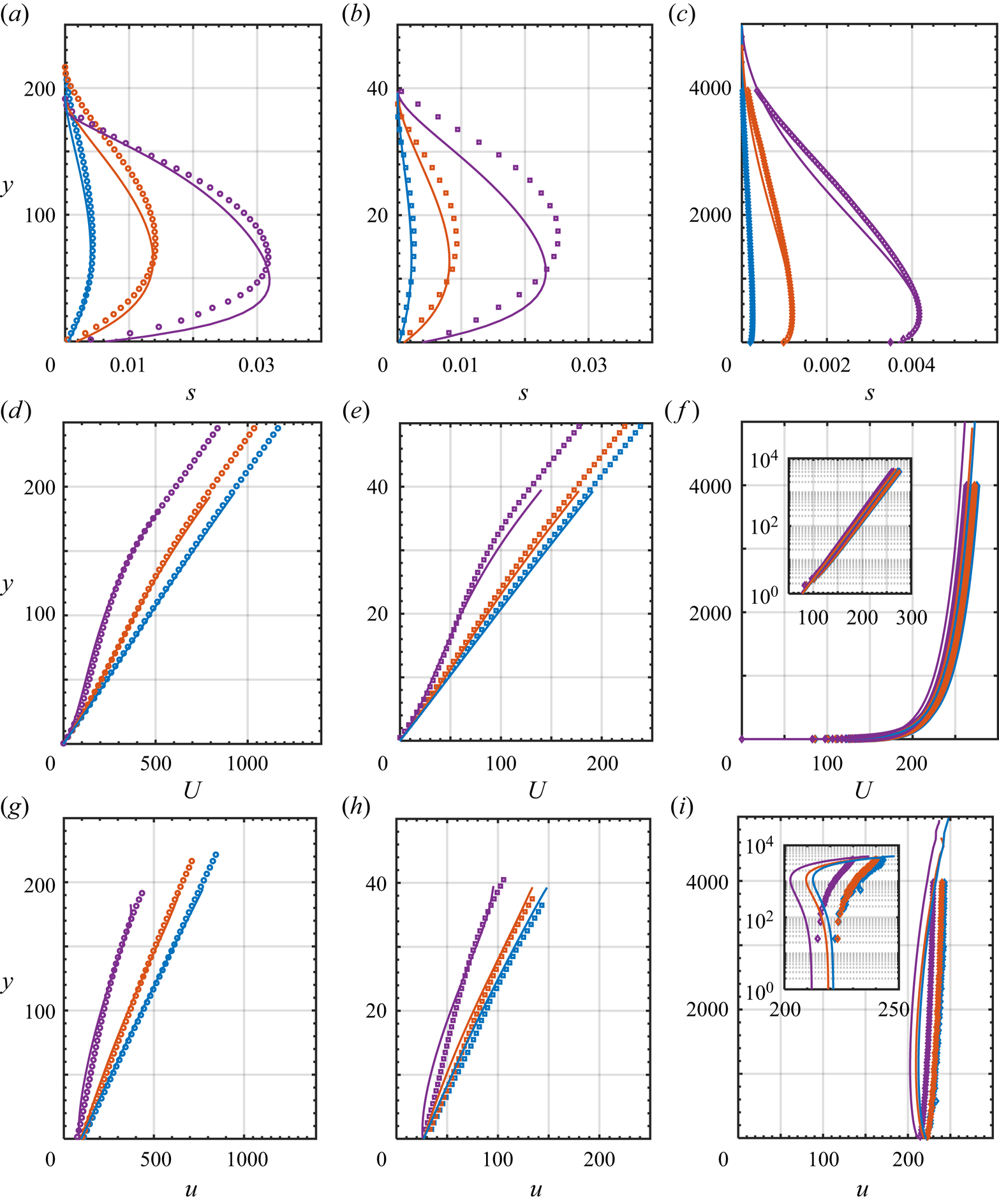
Figure 6. Profiles of (a–c) particle shear stress, (d–f) fluid and (g–i) particle mean horizontal velocities measured in numerical simulations of: saltation in viscous shearing flows with dw = 1, St = 100, r = 150 000, Sh = 0.05 (first column) and M = 0.0008 (blue circles), M = 0.0033 (red circles), M = 0.0131 (purple circles); saltation in viscous shearing flows with dw = 1, St = 100, r = 50, Sh = 0.05 (second column) and M = 0.0008 (blue squares), M = 0.0033 (squares), M = 0.0131 (purple squares); saltation in turbulent shearing flows with dw = 1.5, St = 1681, r = 2208, Sh = 0.04 (third column) and M = 0.0008 (blue diamonds), M = 0.0033 (red diamonds), M = 0.0119 (purple diamonds). The solid lines are the predictions of the present theory. The insets of figures 6(f) and 6(i) show the corresponding velocity profiles in semi-log scale.
In determining the semi-analytical solution that we have highlighted in § 2, we have employed αu = 0.60 and αT = 0.50 for saltation in viscous flows, and αu = 0.85 and αT = 0.18 for saltation in turbulent flows. We have fitted these values to exactly match the depth of the saltation layer, h, and the particle shear stress at the bed, s 0, in one of the discrete simulations of saltation in viscous flows and one of the simulations of saltation in turbulent flows. Different values of these parameters would not alter the qualitative features of our semi-analytical solution, but impact the values of Ty, c and u at the bed, therefore causing a shift to the right or to the left in the relative profiles. As an overall estimate of their influence, we checked that a ten per cent change in either of the alphas would result in a ten per cent change in the mass flux.
Figures 5(a)–5(c) confirm that the intensity of the velocity fluctuations of the particles decreases linearly with the distance from the rigid bed, and that the model captures both the weak dependence of Ty on M for viscous saltation and Stokes drag (figure 5a), and its independence for nonlinear drag (figures 5b and 5c). The depth of the saltation layer is well predicted by the continuum model, but the slope of the linear decrease is underestimated with respect to the numerical simulations for nonlinear drag. Also, the non-monotonic behaviour of Ty near the rigid bed is not captured. These are the consequences of neglecting the dependence of the drag coefficient on the vertical direction. The agreement with the measurements in the numerical simulations would indeed improve if CD is allowed to vary locally; however, this would prevent obtaining semi-analytical solutions of the governing equations, with little improvement on the results. The condition  ${C_D}\sqrt {{T_y}} > 1$ that ensures that the assumption of large vertical velocities of ascending particles with respect to the settling velocity is sufficiently accurate, is satisfied in the flows of figures 5 and 6 everywhere, but for the upper quarter of the flow, where indeed the deviations between the simulations and the predictions are more significant.
In all cases, the continuum model satisfactorily reproduces the profiles of particle concentration and normal stress in the y-direction (figure 5d–i), which indeed follow the power-law distributions of (2.17) and (2.18). In the turbulent case, as anticipated, the particle concentration is rather uniform across the flow (figure 5f). The values of the particle concentration are also much smaller in the case of turbulent shearing flows (figure 5f), as a consequence of the greater agitation of the particles (figure 5c).
Figure 5 shows profiles of quantities associated with the vertical motion of the saltating particles, which is sensitive to the horizontal motion of the fluid only through the dependence of the drag coefficient on U. The horizontal motion of the fluid and, in particular, its flow regime, strongly affects the distribution of particle shear stress and particle and fluid horizontal velocity shown in figure 6.
The proposed constitutive relations for the particle shear stress ((2.25) and (2.38)) permit the qualitative and quantitative reproduction of the measurements in numerical simulations (figure 6a–c). In particular, the position and the magnitude of the peak in the particle shear stress are well captured. The physical reason for the presence of this maximum value of the particle shear stress above the bed is in the change of sign of the horizontal force exerted by the fluid on the particles. The particles slip at the rigid bed, while the fluid does not; hence, the particles drag the fluid near the bed, while the fluid drags the particles as the top of the saltation layer is approached. Interestingly, the particle shear stress can reach values up to 50 %–60 % of the total shear stress – the Shields parameter – for saltation in viscous shearing flows, but only up to 10 % of the total shear stress for saltation in turbulent shearing flows.
For saltation in viscous shearing flows (Figure 6d–h), the fluid and particle horizontal velocity profiles become progressively nonlinear as the particle hold-up increases; but the continuum model is capable of capturing this behaviour. For saltation in turbulent shearing flows, the fluid velocity profile is logarithmic, and the hold-up has little influence on it (figure 6f). The horizontal velocity of the particles is almost uniform vertically (figure 6i). This confirms our finding that, in the absence of particle interactions, the particle shear stress does not depend on the particle shear rate. The slight discrepancies between the predictions of the continuum model and the results of the numerical simulations are likely due to the assumption of a drag coefficient independent of y.
Finally, we compare the dependence of the particle flux on the particle hold-up in figure 7. The continuum model notably reproduces the measurements in numerical simulations in both the viscous and turbulent shearing flows. The experimental results on turbulent saltation in a wind tunnel (Ho Reference Ho2012) are in relatively good agreement with both the numerical simulations and the continuum model (figure 7b). The overestimate of the experimental mass flux is likely due to the additional resistance induced by the presence of the horizontal lid above the rigid bed. Figure 7(a) also assesses the validity of the scaling for q reported in table 1 for the case of viscous saltation and Stokes drag, in the rarefied limit.
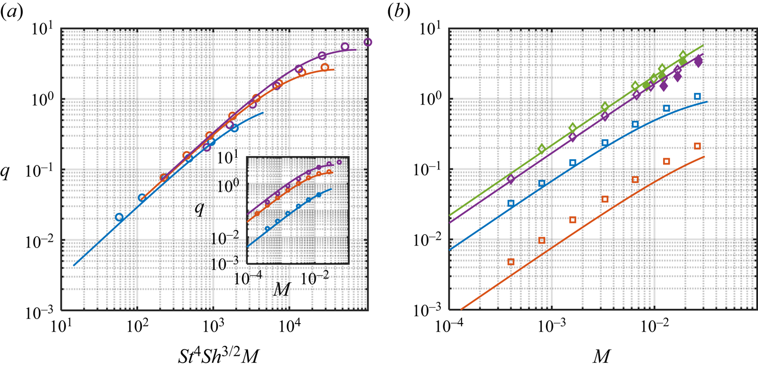
Figure 7. (a) Particle flux against scaled particle hold-up measured in DC numerical simulations (open symbols) and predicted from the present theory (lines) in the case of saltation in viscous shearing flows with dw = 1, r = 150 000 and: St = 60 and Sh = 0.05 (blue circles); St = 100 and Sh = 0.05 (orange circles); St = 100 and Sh = 0.075 (purple circles). The inset depicts the same data in terms of q against M. (b) Particle flux against particle hold-up measured in DC numerical simulations (open symbols) and in wind-tunnel experiments (filled symbols, after Ho Reference Ho2012) and predicted from the present theory (lines) in the case of saltation in viscous shearing flows with dw = 1, St = 100 Sh = 0.05 and r = 2.5 (orange squares) and r = 50 (blue squares); and in the case of saltation in turbulent shearing flows with dw = 1.5, St = 1681, r = 2208 and Sh = 0.025 (purple diamonds) and Sh = 0.04 (green diamonds).
5. Conclusions
We have derived constitutive relations for the particle stresses and flux of particle kinetic energy associated with the fluctuating vertical velocities that apply to saltation of particles in viscous and turbulent shearing flows, in the absence of collisions above the bed. To do this, we have employed the averaging methods of statistical mechanics based on an anisotropic Maxwellian velocity distribution function for the ascending particles and approximate analytical expressions for the particle trajectories under the influence of fluid drag, gravity and buoyancy, in the limit of large vertical velocity of ascending particles relative to the settling velocity.
Given that we neglect the possibility of particle–particle interactions, we have obtained the perhaps unexpected result that the particle shear stress does depend on the local relative velocity between the grains and the carried fluid and the fluid shear rate, but not on the particle shear rate. We have combined the constitutive relations for the particle phase and well-known expressions for the fluid shear stress with momentum and energy balances to obtain semi-analytical solutions of steady, fully developed saltation over horizontal, rigid beds. We have employed boundary conditions appropriated for particles rebounding at a bumpy base with no upper bound to the flow. We have assumed that the carrier fluid has only mean horizontal velocity. Hence, the regime of the carrier fluid, viscous or turbulent, does not affect the profiles of particle concentration and normal stress, which follow a power-law decrease with height, and mean square of the vertical velocity fluctuations, linearly decreasing with the distance from the bed. These results are in contrast with previous theoretical (e.g. Jenkins et al. Reference Jenkins, Cantat and Valance2010; Jenkins & Valance Reference Jenkins and Valance2014) and experimental (Creyssels et al. Reference Creyssels, Dupont, Ould El Moctar, Valance, Cantat, Jenkins, Pasini and Rasmussen2009) works in which the granular temperature was assumed to be uniform and the concentration was shown to decrease exponentially with height.
We have confirmed our findings through a number of comparisons with DC simulations in both viscous and turbulent regimes. Thus, we are inclined to blame mid-fluid collisions for the above mentioned qualitative difference in the distribution of particle concentration. We have also shown that the predictions of the theory in terms of profiles of particle shear stress, and particle and fluid mean horizontal velocities, are in excellent agreement with the numerical simulations. In natural units of particle mass density, diameter and reduced gravity, we have determined that the saltation process is controlled by the mass of particles in the system, the intensity of the shearing flow, the fluid mass density and viscosity and the bumpiness of the rigid base.
We have successfully tested the dependence of the horizontal particle flux per unit basal area of the particles as a function of the particle hold-up obtained with our theory against DC numerical simulations and wind-tunnel experiments, for a large range of the control parameters. We have also determined simple scaling laws for the dependence of various quantities of interest on the control variables in the special limits of rarefied viscous and turbulent saltation, and solely Stokes or form drag on the particles.
In a future, we plan to apply our theory to two-point boundary value problems, to e.g. mimic available experiments of saltation in enclosed wind tunnels. We also wish to extend the present work to deal with unsteady and/or developing flows. More importantly, the inclusion of mid-fluid collisions, that is the transition from a collisionless to a collisional kinetic theory of saltation, is a crucial future step, especially in view of modelling transport phenomena over erodible beds, of more interest for geophysical and planetary science applications.
Acknowledgements
We are grateful to T. Pähtz for comments on the manuscript that led to its improvement.
Funding
J.T.J. was supported in part by a Podell Endowment Award for Research and Scholarship from Cornell University. A.V. acknowledges the support of the French Research National Agency through the project ANR-21-CE30–0066.
Declaration of interests
The authors report no conflict of interest.
Appendix A. Approximate analytical trajectories for the saltating particles
We characterize the drag exerted on the particles through a drag coefficient, CD, that we take to be independent of y, as in Pasini & Jenkins (Reference Pasini and Jenkins2005), to obtain analytical expressions for the particle trajectories.
Integrating the vertical momentum balance for the particle
 \begin{equation}\frac{{\textrm{d}{\xi _y}}}{{\textrm{d}t}} + {C_D}{\xi _y} + 1 = 0,\end{equation}
with ξy the vertical component of the particle velocity, we obtain the vertical velocity at any time t after the particle reaches a certain ascending velocity  $\xi _y^ +$ at a certain location yr
 \begin{equation}{\xi _y} = \frac{{{C_D}\xi _y^ + + 1 - \exp ({C_D}t)}}{{{C_D}\exp ({C_D}t)}};\end{equation}
and, with another integration, the position y as a function of time
 \begin{equation}y - {y_r} = \frac{{({C_D}\xi _y^ + + 1)[1 - \exp ( - {C_D}t)] - {C_D}t}}{{C_D^2}}.\end{equation}
From (A3) we obtain an implicit expression for the time that the particle spends at y ≥ yr
 \begin{equation}{t_f} = \frac{{{C_D}\xi _y^ + + 1}}{{{C_D}}}[1 - \exp ( - {C_D}{t_f})].\end{equation}
Then, from (A2), with t = tf, the downward vertical velocity of the particle at y = yr is
 \begin{equation}\xi _y^ - = \xi _y^ + - {t_f}.\end{equation}
To permit subsequent analytical integrations, we propose the following explicit expression for the time of flight
 \begin{equation}{t_f} = \xi _y^ + + \frac{1}{{{C_D}}} - \frac{1}{{{C_D}}}\exp ( - {C_D}\xi _y^ + ),\end{equation}
which has the right limits at both small  ${C_D}\xi _y^ +$, i.e.
  ${t_f} = 2\xi _y^ +$, and large
  ${C_D}\xi _y^ +$, i.e.
  ${t_f} = \xi _y^ + + C_D^{ - 1}$. With this, (A5) gives
 \begin{equation}\xi _y^ - = - \frac{1}{{{C_D}}} + \frac{1}{{{C_D}}}\exp ( - {C_D}\xi _y^ + ).\end{equation}
In the limit of large  ${C_D}\xi _y^ +$, (A7) reduces to
 \begin{equation}\xi _y^ - = - \frac{1}{{{C_D}}}.\end{equation}
We next integrate the horizontal particle momentum balances, and distinguish between saltation in viscous and in turbulent shearing flows.
A.1. Saltation in viscous shearing flows
In the case of saltation in viscous shearing flows, we assume that the fluid velocity profile is locally linear (that is for y ≥ yr), so that the horizontal momentum balance for the particles is
 \begin{equation}\frac{{\textrm{d}{\xi _x}}}{{\textrm{d}t}} = {C_D}\left[ {U + \frac{{\textrm{d}U}}{{\textrm{d}y}}(y - {y_r}) - {\xi_x}} \right],\end{equation}
with ξx the horizontal component of the particle velocity, and U and  $\textrm{d}U/\textrm{d}y$ the fluid horizontal velocity and shear rate at the reference level. In the following integrations, we treat
  $\textrm{d}U/\textrm{d}y$ for saltation in viscous shearing flows as if it were constant. Then, after inserting equation (A3) into (A9), and integrating with the initial condition
  ${\xi _x}(t = 0) = \xi _x^ +$
 \begin{align} {\xi _x} & = U +
\dfrac{{\textrm{d}U}}{{\textrm{d}y}}\dfrac{{({C_D}\xi _y^ + + 1)}}{{C_D^2}}[1 - {C_D}t{\rm exp} ( - {C_D}t) -
\exp ( - {C_D}t)]\nonumber\notag\\ & \quad - \dfrac{{\textrm{d}U}}{{\textrm{d}y}}\dfrac{{{C_D}t - 1 + \exp ( -
{C_D}t)}}{{C_D^2}} + (\xi _x^ + - U)\exp ( - {C_D}t). \end{align}
\begin{align} {\xi _x} & = U +
\dfrac{{\textrm{d}U}}{{\textrm{d}y}}\dfrac{{({C_D}\xi _y^ + + 1)}}{{C_D^2}}[1 - {C_D}t{\rm exp} ( - {C_D}t) -
\exp ( - {C_D}t)]\nonumber\notag\\ & \quad - \dfrac{{\textrm{d}U}}{{\textrm{d}y}}\dfrac{{{C_D}t - 1 + \exp ( -
{C_D}t)}}{{C_D^2}} + (\xi _x^ + - U)\exp ( - {C_D}t). \end{align}
The horizontal velocity after the time tf is, then, with (A4) and (A6)
 \begin{align} \xi _x^ - & = U +
\dfrac{1}{{C_D^2}}\dfrac{{\textrm{d}U}}{{\textrm{d}y}}\dfrac{1}{{{C_D}\xi _y^ + + 1}}[{C_D}\xi _y^ + + 1
- \exp ( - {C_D}\xi _y^ + )][1 - \exp ( - {C_D}\xi _y^ + )\nonumber\notag\\ & \quad - {C_D}\xi _y^ + \exp ( - {C_D}\xi _y^ +
)] + \dfrac{{{\xi _x^{+}} - U}}{{{C_D}\xi _y^ + + 1}}\exp ( - {C_D}\xi _y^ + ),
\end{align}
\begin{align} \xi _x^ - & = U +
\dfrac{1}{{C_D^2}}\dfrac{{\textrm{d}U}}{{\textrm{d}y}}\dfrac{1}{{{C_D}\xi _y^ + + 1}}[{C_D}\xi _y^ + + 1
- \exp ( - {C_D}\xi _y^ + )][1 - \exp ( - {C_D}\xi _y^ + )\nonumber\notag\\ & \quad - {C_D}\xi _y^ + \exp ( - {C_D}\xi _y^ +
)] + \dfrac{{{\xi _x^{+}} - U}}{{{C_D}\xi _y^ + + 1}}\exp ( - {C_D}\xi _y^ + ),
\end{align}
which in the limit of large  ${C_D}\xi _y^ +$ gives
 \begin{equation}\xi _x^ - = U + \frac{1}{{C_D^2}}\frac{{\textrm{d}U}}{{\textrm{d}y}}.\end{equation}
Equation (A10) can be integrated with the boundary condition x(t = 0) = xi to obtain the horizontal displacement from the initial position at the reference level as a function of time
 \begin{align}\begin{aligned} x & = {x_i} + Ut +
\dfrac{{({C_D}\xi _y^ + + 1)}}{{C_D^2}}\dfrac{{\textrm{d}U}}{{\textrm{d}y}}\left[ {\exp ( - {C_D}t)\left(
{\dfrac{2}{{{C_D}}} + t} \right) + t - \dfrac{2}{{{C_D}}}} \right]\nonumber\cr & \quad -
\dfrac{1}{{C_D^2}}\dfrac{{\textrm{d}U}}{{\textrm{d}y}}\left[ {\dfrac{{{C_D}{t^2}}}{2} - t -
\dfrac{1}{{{C_D}}}\exp ( - {C_D}t) + \dfrac{1}{{{C_D}}}} \right] + \dfrac{1}{{{C_D}}}(\xi _x^ + - U)[1 -
\exp ( - {C_D}t)]. \end{aligned}\end{align}
\begin{align}\begin{aligned} x & = {x_i} + Ut +
\dfrac{{({C_D}\xi _y^ + + 1)}}{{C_D^2}}\dfrac{{\textrm{d}U}}{{\textrm{d}y}}\left[ {\exp ( - {C_D}t)\left(
{\dfrac{2}{{{C_D}}} + t} \right) + t - \dfrac{2}{{{C_D}}}} \right]\nonumber\cr & \quad -
\dfrac{1}{{C_D^2}}\dfrac{{\textrm{d}U}}{{\textrm{d}y}}\left[ {\dfrac{{{C_D}{t^2}}}{2} - t -
\dfrac{1}{{{C_D}}}\exp ( - {C_D}t) + \dfrac{1}{{{C_D}}}} \right] + \dfrac{1}{{{C_D}}}(\xi _x^ + - U)[1 -
\exp ( - {C_D}t)]. \end{aligned}\end{align}
The horizontal displacement Δ after the time tf is
 \begin{align}\begin{aligned} \varDelta & = U{t_f} + \dfrac{{({C_D}\xi _y^ + + 1)}}{{C_D^2}}\dfrac{{\textrm{d}U}}{{\textrm{d}y}}\left[ {\exp ( - {C_D}{t_f})\left( {\dfrac{2}{{{C_D}}} + {t_f}} \right) + {t_f} - \dfrac{2}{{{C_D}}}} \right]\nonumber\cr & \quad - \dfrac{1}{{C_D^2}}\dfrac{{\textrm{d}U}}{{\textrm{d}y}}\left[ {\dfrac{{{C_D}t_f^2}}{2} - {t_f} - \dfrac{1}{{{C_D}}}\exp ( - {C_D}{t_f}) + \dfrac{1}{{{C_D}}}} \right] + \dfrac{1}{{{C_D}}}(\xi _x^ + - U)[1 - \exp ( - {C_D}{t_f})]. \end{aligned}\end{align}
In the limit of large  ${C_D}\xi _y^ +$,
  ${t_f} = \xi _y^ + + C_D^{ - 1}$ and (A14) reduces to
 \begin{equation}\varDelta = \frac{1}{{2{C_D}}}\frac{{\textrm{d}U}}{{\textrm{d}y}}\xi _y^{ + 2} + U\xi _y^ + + \frac{{\xi _x^ + - U}}{{{C_D}}}.\end{equation}
A.2. Saltation in turbulent shearing flows
In the case of saltation in turbulent shearing flows, we assume that the fluid velocity above a reference location yr is the classical logarithmic,  $U + \sqrt {rS} \ln [1 + \kappa (\textrm{d}U/\textrm{d}y)(y - {y_r})/\sqrt {rS} ]/\kappa$, obtained by integrating equation (2.44) with the assumption that the fluid shear stress S is independent of y, in which U and
  $\textrm{d}U/\textrm{d}y$ are the fluid horizontal velocity and shear rate at the reference level. Then, the horizontal momentum balance for the particles reads, with (A3)
 \begin{align}\frac{{\textrm{d}{\xi _x}}}{{\textrm{d}t}} = {C_D}U + {C_D}\frac{{\sqrt {rS} }}{\kappa }\ln \left\{ {1 + \frac{\kappa }{{\sqrt {rS} }}\frac{{({C_D}\xi_y^ + + 1)[1 - \exp ( - {C_D}t)] - {C_D}t}}{{C_D^2}}\frac{{\textrm{d}U}}{{\textrm{d}y}}} \right\} - {C_D}{\xi _x}.\end{align}
 After integrating equation (A16) with the initial condition  ${\xi _x}(t = 0) = \xi _x^ +$
 \begin{align}\begin{aligned} {\xi _x} & = \xi _x^ + \exp ( - {C_D}t) + U[1 - \exp ( - {C_D}t)] + \dfrac{{\sqrt {rS} }}{\kappa }\exp ( - {C_D}t)\nonumber\cr & \quad \times \int_0^{{C_D}t} {\exp ({C_D}t)\ln \left\{ {1 + \kappa \dfrac{{({C_D}\xi_y^ + + 1)[1 - \exp ( - {C_D}t)] - {C_D}t}}{{C_D^2\sqrt {rS} }}\dfrac{{\textrm{d}U}}{{\textrm{d}y}}} \right\}{\rm d}({C_D}t)} . \end{aligned}\end{align}
The horizontal velocity after the time tf is, then,
 \begin{align}\begin{aligned} \xi _x^ - & = \xi _x^ + \exp ( - {C_D}{t_f}) + U[1 - \exp ( - {C_D}{t_f})] + \dfrac{{\sqrt {rS} }}{\kappa }\exp ( - {C_D}{t_f})\nonumber\cr & \quad \times \int_0^{{C_D}{t_f}} {\exp ({C_D}t)\ln \left\{ {1 + \kappa \dfrac{{({C_D}\xi_y^ + + 1)[1 - \exp ( - {C_D}t)] - {C_D}t}}{{{C_D^2}\sqrt {rS} }}\dfrac{{\textrm{d}U}}{{\textrm{d}y}}} \right\}{\rm d}({C_D}t)} . \end{aligned}\end{align}
In the limit of large  ${C_D}\xi _y^ +$, that is large
  ${C_D}{t_f}$, (A18), with (A6), gives the following analytical solution:
 \begin{align}\xi _x^ - & = U + \exp ( - {C_D}{t_f})\dfrac{{\sqrt {rS} }}{\kappa }\int_0^{{C_D}{t_f}} {\exp ({C_D}t)\ln \left( {1 + \dfrac{{{C_D}{t_f} - {C_D}t}}{{C_D^2\dfrac{{\sqrt {rS} }}{\kappa }}}\dfrac{{\textrm{d}U}}{{\textrm{d}y}}} \right){\rm d}({C_D}t)} \nonumber\notag\\ & = U - \dfrac{{\sqrt {rS} }}{\kappa }\exp \left[ {C_D^2\dfrac{{\sqrt {rS} }}{\kappa }{{\left( {\dfrac{{\textrm{d}U}}{{\textrm{d}y}}} \right)}^{ - 1}}} \right]Ei\left[ { - C_D^2\dfrac{{\sqrt {rS} }}{\kappa }{{\left( {\dfrac{{\textrm{d}U}}{{\textrm{d}y}}} \right)}^{ - 1}}} \right], \end{align}
in which  $Ei(x) \equiv{-} \int_{ - x}^\infty {{e^{ - t}}{t^{ - 1}}\,{\rm d}t} $ is the exponential integral.
Appendix B. Constitutive relations
We define the average of a quantity φ at a certain distance y from the bed as
 \begin{equation}\langle \varphi \rangle = \frac{\rm \pi}{{6c}}\int_{all\;\xi } {\varphi f\,{\textrm{d}^2}\boldsymbol{\xi} } = \frac{\rm \pi}{{6c}}\int_{all\;{\xi ^ + }} {{\varphi ^ + }{f^ + }\,{\textrm{d}^2}{\boldsymbol{\xi} ^ + }} + \frac{\rm \pi}{{6c}}\int_{all\;{\xi ^ - }} {{\varphi ^ - }{f^ - }\,{\textrm{d}^2}{\boldsymbol{\xi} ^ - }} ,\end{equation}
where f is the velocity distribution of particles at that height and 6c/ ${\rm \pi}$ is the dimensionless number density. As in Creyssels et al. (Reference Creyssels, Dupont, Ould El Moctar, Valance, Cantat, Jenkins, Pasini and Rasmussen2009), we distinguish between ascending or descending particles and introduce velocity distributions for both species. We assume that the velocity distribution of the ascending particles is an anisotropic Maxwellian
 \begin{equation}{f^ + } = \frac{6}{\rm \pi}\frac{{{c^ + }}}{{{\rm \pi}\sqrt {T_x^ + T_y^ + } }}\exp \left[ { - \frac{{{{(\xi_x^ + - u)}^2}}}{{2T_x^ + }}} \right]\exp \left( { - \frac{{\xi_y^{ + 2}}}{{2T_y^ + }}} \right),\end{equation}
where  $u = \langle {\xi _x}\rangle$ and
  $T_x^ + = ({\rm \pi}/6{c^ + })\int_{all\;{\xi ^ + }} {{{({\xi _x^ +} - u)}^2}{f^ + }\,{\textrm{d}^2}{\boldsymbol{\xi} ^ + }}$ and
  $T_y^ + = ({\rm \pi}/6{c^ + })\int_{all\;{\xi ^ + }} {\xi _y^{+2}} {f^ + }\,{{\rm d}^2}{\boldsymbol{\xi} ^ + }$ are the mean squares of the horizontal velocity fluctuations of the ascending particles. The concentration of the ascending particles, c +, is equal to
  $({\rm \pi}/6)\int_{all\;{\xi ^ + }} {{f^ + }\,{\textrm{d}^2}{\boldsymbol{\xi} ^ + }}$, while that of the descending particle is
  ${c^ - } = ({\rm \pi}/6)\int_{all\;{\xi ^ - }} {{f^ - }\,{\textrm{d}^2}{\boldsymbol{\xi} ^ - }}$. When
  $\varphi = 1$, (B1) gives
  $c = {c^ + } + {c^ - }$.
Given that we are dealing with steady states,  $\langle {\xi _y}\rangle = 0$, so that
 \begin{equation}\langle {\xi _y}\rangle
= \frac{\rm \pi}{{6c}}\int_{all\;{\boldsymbol{\xi} ^ + }} {{\xi _y^ +} {f^
+ }\,{\textrm{d}^2}{\boldsymbol{\xi} ^ + }} +
\frac{\rm \pi}{{6c}}\int_{all\;{\boldsymbol{\xi} ^ - }} {{\xi _y^ -} {f^ -
}\,{\textrm{d}^2}{\boldsymbol{\xi} ^ - }} =
0.\end{equation}
\begin{equation}\langle {\xi _y}\rangle
= \frac{\rm \pi}{{6c}}\int_{all\;{\boldsymbol{\xi} ^ + }} {{\xi _y^ +} {f^
+ }\,{\textrm{d}^2}{\boldsymbol{\xi} ^ + }} +
\frac{\rm \pi}{{6c}}\int_{all\;{\boldsymbol{\xi} ^ - }} {{\xi _y^ -} {f^ -
}\,{\textrm{d}^2}{\boldsymbol{\xi} ^ - }} =
0.\end{equation}
Then, we take the limit for large  ${C_D}\xi _y^ +$ of
  $\xi _y^ -$ (A9) and, inserting equation (B2) into (B3), and integrating, we obtain
 \begin{equation} {c^ + }{C_D}\sqrt
{\dfrac{{2{T_y}^ + }}{\rm \pi}} = {c^ - }.
\end{equation}
\begin{equation} {c^ + }{C_D}\sqrt
{\dfrac{{2{T_y}^ + }}{\rm \pi}} = {c^ - }.
\end{equation}
This is a relation between the concentrations of the two species of particles. As shown later, we find that (B4) does not capture the correct limit as  $T_y^ + $ tends to zero, and also slightly underestimates c −. This is because the limit of large take-off velocity does not capture the fact that the vertical velocity of the descending particles near the top of the saltation layer is less than the settling velocity. An almost perfect agreement can be obtained, instead, with
 \begin{equation}{c^ - } = {c^ + } + \frac{3}{4}{c^ + }{C_D}\sqrt {\frac{{2T_y^ + }}{\rm \pi}} .\end{equation}
From this and the definition of c
 \begin{equation}c = {c^ + } + {c^ - } = {c^ + }\left( {2 + \frac{3}{4}{C_D}\sqrt {\frac{{2T_y^ + }}{\rm \pi}} } \right).\end{equation}
Taking the limit for large  ${C_D}\xi _y^ +$ permits (B4)–(B6) to be obtained without assuming a velocity distribution for the descending particles. We show the comparisons between (B5) and (B6) and the results of numerical simulations on saltation of particles in a viscous shearing flow experiencing Stokes drag in figure 8.
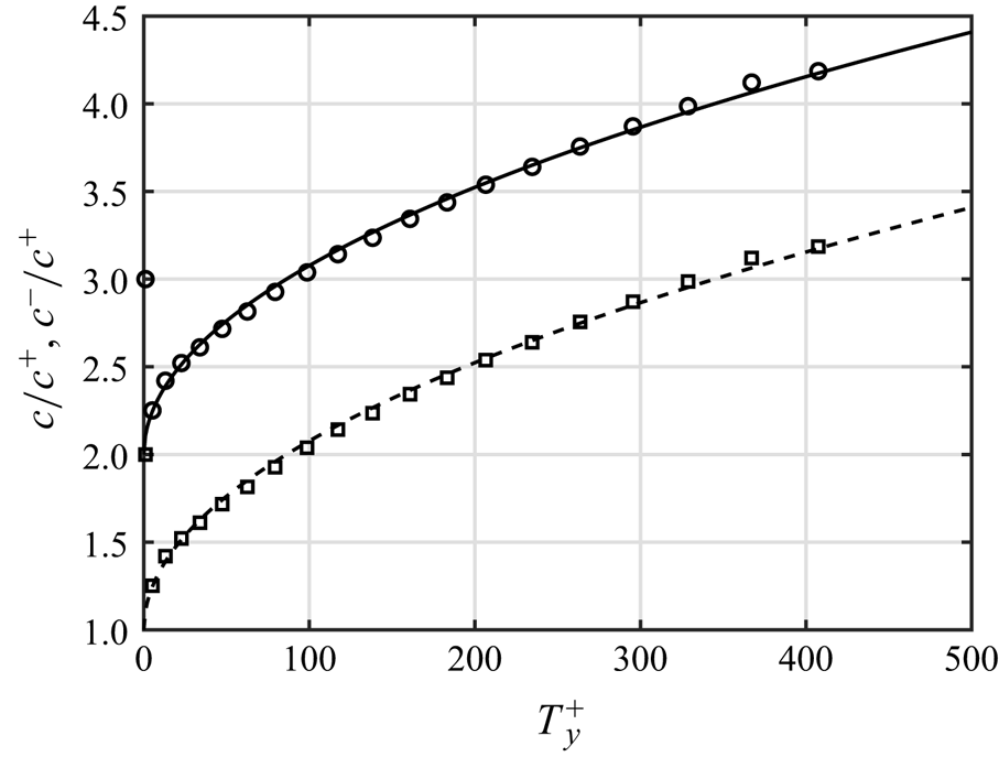
Figure 8. Concentration ratios c/c + (circles) and c −/c + (squares) as functions of  $T_y^ + $ measured in numerical simulations of saltation in a viscous shearing flow with dw = 1, St = 100, r = 150 000, Sh = 0.05 (so that the Stokes drag is dominant and CD = 18/St = 0.18) and M = 0.0131. The dashed and solid lines are the predictions of (B5) and (B6), respectively.
Equation (B1) can be rewritten as
 \begin{align}\langle \varphi \rangle & =
\dfrac{\rm \pi}{{6c}}\int_{all\;{\xi ^ + }} {{\varphi ^ + }{f^
+ }\,{\textrm{d}^2}{\boldsymbol{\xi} ^ + }} +
\dfrac{\rm \pi}{{6c}}\int_{all\;{\xi ^ - }} {{\varphi ^ - }{f^
- }\,{\textrm{d}^2}{\boldsymbol{\xi} ^ - }}\nonumber\\ &=
\dfrac{\rm \pi}{{6c}}\int_{all\;{\xi ^ + }} {{\varphi ^ + }{f^
+ }\,{\textrm{d}^2}{\boldsymbol{\xi} ^ + }} +
\dfrac{\rm \pi}{{6c}}\int_{all\;{\xi ^ + }} {{\varphi ^ - }{f^
- }|{J^ - }|\,{\textrm{d}^2}{\boldsymbol{\xi} ^ + }} \nonumber\\ & =
\dfrac{\rm \pi}{{6c}}\int_{all\;{\xi ^ + }}
{\textrm{[}{\varphi ^ + }{f^ + } + {\varphi ^ - }{f^ -
}\textrm{|}{J^ - }|]\,{\textrm{d}^2}{\boldsymbol{\xi} ^ + }} ,
\end{align}
\begin{align}\langle \varphi \rangle & =
\dfrac{\rm \pi}{{6c}}\int_{all\;{\xi ^ + }} {{\varphi ^ + }{f^
+ }\,{\textrm{d}^2}{\boldsymbol{\xi} ^ + }} +
\dfrac{\rm \pi}{{6c}}\int_{all\;{\xi ^ - }} {{\varphi ^ - }{f^
- }\,{\textrm{d}^2}{\boldsymbol{\xi} ^ - }}\nonumber\\ &=
\dfrac{\rm \pi}{{6c}}\int_{all\;{\xi ^ + }} {{\varphi ^ + }{f^
+ }\,{\textrm{d}^2}{\boldsymbol{\xi} ^ + }} +
\dfrac{\rm \pi}{{6c}}\int_{all\;{\xi ^ + }} {{\varphi ^ - }{f^
- }|{J^ - }|\,{\textrm{d}^2}{\boldsymbol{\xi} ^ + }} \nonumber\\ & =
\dfrac{\rm \pi}{{6c}}\int_{all\;{\xi ^ + }}
{\textrm{[}{\varphi ^ + }{f^ + } + {\varphi ^ - }{f^ -
}\textrm{|}{J^ - }|]\,{\textrm{d}^2}{\boldsymbol{\xi} ^ + }} ,
\end{align}
where J − is the Jacobian of the transformation from  ${\boldsymbol{\xi} ^ + }$ into
  ${\boldsymbol{\xi} ^ - }$. When we calculate the average vertical flux of the generic quantity
 \begin{align}\langle \varphi {\xi _y}\rangle = \frac{\rm \pi}{{6c}}\int_{all\;{\xi ^ + }} {[{\varphi ^ + }\xi _y^ + {f^ + } + {\varphi ^ - }\boldsymbol{\xi} _y^ - {f^ - }|{J^ - }|]\,{\textrm{d}^2}{\boldsymbol{\xi} ^ + }} = \frac{\rm \pi}{{6c}}\int_{all\;{\xi ^ + }} {[{\varphi ^ + } - {\varphi ^ - }]\xi _y^ + {f^ + }\,{\textrm{d}^2}{\boldsymbol{\xi} ^ + }} ,\end{align}
where we made use of the fact that, at steady state,  $\langle {\xi _y}\rangle = 0$ and, therefore, from (B3), if the trajectories are independent of each other (that is for small particle hold-ups),
  $\xi _y^ + {f^ + } = - \xi _y^- {f^ - }|{J^ - }|$ (Pasini & Jenkins Reference Pasini and Jenkins2005).
The particle normal stress in the y-direction, in the absence of particle interaction, is simply given by the average vertical flux of y-momentum,  ${\sigma _y} \equiv c\langle {\xi _y}{\xi _y}\rangle = c{T_y}$, where
  ${T_y} = \langle \xi _y^2\rangle$ is the mean square of the vertical velocity fluctuation for all the particles. However, using (B8)
 \begin{equation}{\sigma _y} = \frac{\rm \pi}{6}\int_0^{ + \infty } {\int_{ - \infty }^{ + \infty } (\xi _y^ + - \xi _y^ - )\xi _y^ + {f^ + }\,\textrm{d}\xi _x^ + \,\textrm{d}\xi _y^ + } .\end{equation}
Then, upon taking the limit for large  ${C_D}\xi _y^ +$ of
  $\xi _y^ -$ (A8) and, inserting equation (B2) into (B9), and integrating, we obtain
 \begin{align} {\sigma _y} & =
\dfrac{{{c^ + }}}{{{\rm \pi}\sqrt {T_x^ + T_y^ + } }}\int_0^{ +
\infty } {\left( {\xi_y^ + + \dfrac{1}{{{C_D}}}} \right)\xi
_y^ + \exp \left( { - \dfrac{{\xi_y^{ + 2}}}{{2T_y^ + }}}
\right)} \int_{ - \infty }^{ + \infty } {\exp \left[ { -
\dfrac{{{{(\xi_x^ + - u)}^2}}}{{2T_x^ + }}}
\right]\,\textrm{d}\xi _x^ + \,\textrm{d}\xi _y^ + }
\nonumber\\ & = \dfrac{{{c^ + }}}{{{\rm \pi}\sqrt {T_x^ + T_y^
+ } }}\sqrt {2{\rm \pi} T_x^ + } \int_0^{ + \infty } {\left( {\xi_y^
+ + \dfrac{1}{{{C_D}}}} \right)\xi _y^ + \exp \left( { -
\dfrac{{\xi_y^{ + 2}}}{{2T_y^ + }}} \right)\textrm{d}\xi
_y^ + }\nonumber\\ &= {c^ + }T_y^ + + {c^ +
}\dfrac{1}{{{C_D}}}\sqrt {\dfrac{{2T_y^ + }}{\rm \pi}} .
\end{align}
\begin{align} {\sigma _y} & =
\dfrac{{{c^ + }}}{{{\rm \pi}\sqrt {T_x^ + T_y^ + } }}\int_0^{ +
\infty } {\left( {\xi_y^ + + \dfrac{1}{{{C_D}}}} \right)\xi
_y^ + \exp \left( { - \dfrac{{\xi_y^{ + 2}}}{{2T_y^ + }}}
\right)} \int_{ - \infty }^{ + \infty } {\exp \left[ { -
\dfrac{{{{(\xi_x^ + - u)}^2}}}{{2T_x^ + }}}
\right]\,\textrm{d}\xi _x^ + \,\textrm{d}\xi _y^ + }
\nonumber\\ & = \dfrac{{{c^ + }}}{{{\rm \pi}\sqrt {T_x^ + T_y^
+ } }}\sqrt {2{\rm \pi} T_x^ + } \int_0^{ + \infty } {\left( {\xi_y^
+ + \dfrac{1}{{{C_D}}}} \right)\xi _y^ + \exp \left( { -
\dfrac{{\xi_y^{ + 2}}}{{2T_y^ + }}} \right)\textrm{d}\xi
_y^ + }\nonumber\\ &= {c^ + }T_y^ + + {c^ +
}\dfrac{1}{{{C_D}}}\sqrt {\dfrac{{2T_y^ + }}{\rm \pi}} .
\end{align}
The limit for large  ${C_D}\xi _y^ +$ permits a simple expression for σy (and for the other constitutive relations) to be obtained. This approximation is valid whenever the Maxwellian vertical velocity distribution of the ascending particles is wide, that is for large
  $T_y^ + $, so that the contribution of the large
  $\xi _y^ +$ is significant. Conversely, it becomes less accurate near the top of the saltating layer, where we expect small values of
  $T_y^ + $ and a subsequent narrower distribution of
  $\xi _y^ +$ around zero. If we use the more accurate equation (A7) in (B9), we would obtain the following constitutive relation for the particle normal stress
 \begin{align}
\sigma _y^\ast & = \dfrac{{{c^ + }}}{{{\rm \pi}\sqrt {T_x^ + T_y^ + } }}\int_0^{ + \infty } \left( {\xi_y^ + + \dfrac{1}{{{C_D}}} -
\dfrac{1}{{{C_D}}}\exp ( - {C_D}\xi_y^ + )} \right)\nonumber\\
&\quad\times \xi _y^ + \exp \left( { - \dfrac{{\xi_y^{ + 2}}}{{2T_y^ + }}} \right) \int_{ - \infty }^{ + \infty } {\exp \left[ { - \dfrac{{{{(\xi_x^ + - u)}^2}}}{{2T_x^ + }}} \right]\textrm{d}\xi _x^ + \,\textrm{d}\xi _y^ + } \nonumber\\
& = \dfrac{{{c^ + }}}{{{\rm \pi}\sqrt {T_x^ + T_y^ + } }}\sqrt {2{\rm \pi} T_x^ + } \int_0^{ + \infty } {\left( {\xi_y^ + + \dfrac{1}{{{C_D}}} -
\dfrac{1}{{{C_D}}}\exp ( - {C_D}\xi_y^ + )} \right)\xi _y^ + \exp \left( { - \dfrac{{\xi_y^{ + 2}}}{{2T_y^ + }}} \right)\textrm{d}\xi _y^ + } \nonumber\\
& = {c^ + }T_y^ + + {c^ + }T_y^ + \exp \left( {\dfrac{{C_D^2T_y^ + }}{2}} \right)erfc\left( {\sqrt {\dfrac{{C_D^2T_y^ + }}{2}} } \right). \end{align}
\begin{align}
\sigma _y^\ast & = \dfrac{{{c^ + }}}{{{\rm \pi}\sqrt {T_x^ + T_y^ + } }}\int_0^{ + \infty } \left( {\xi_y^ + + \dfrac{1}{{{C_D}}} -
\dfrac{1}{{{C_D}}}\exp ( - {C_D}\xi_y^ + )} \right)\nonumber\\
&\quad\times \xi _y^ + \exp \left( { - \dfrac{{\xi_y^{ + 2}}}{{2T_y^ + }}} \right) \int_{ - \infty }^{ + \infty } {\exp \left[ { - \dfrac{{{{(\xi_x^ + - u)}^2}}}{{2T_x^ + }}} \right]\textrm{d}\xi _x^ + \,\textrm{d}\xi _y^ + } \nonumber\\
& = \dfrac{{{c^ + }}}{{{\rm \pi}\sqrt {T_x^ + T_y^ + } }}\sqrt {2{\rm \pi} T_x^ + } \int_0^{ + \infty } {\left( {\xi_y^ + + \dfrac{1}{{{C_D}}} -
\dfrac{1}{{{C_D}}}\exp ( - {C_D}\xi_y^ + )} \right)\xi _y^ + \exp \left( { - \dfrac{{\xi_y^{ + 2}}}{{2T_y^ + }}} \right)\textrm{d}\xi _y^ + } \nonumber\\
& = {c^ + }T_y^ + + {c^ + }T_y^ + \exp \left( {\dfrac{{C_D^2T_y^ + }}{2}} \right)erfc\left( {\sqrt {\dfrac{{C_D^2T_y^ + }}{2}} } \right). \end{align}
The difference between the approximate (B10) and the more accurate (B11) is shown in figure 9(a) when the drag coefficient is equal to 0.18. We see that the mismatch becomes relevant only at small  $T_y^ + $, as expected. The agreement with the measurements in the numerical simulations of saltation of particles in a viscous shearing flow experiencing Stokes drag is remarkable. Figure 9(b) shows the approximation error,
  $|{\sigma _y} - \sigma _y^\ast |/\sigma _y^\ast $, as a function of
  ${C_D}\sqrt {T_y^ + }$, that is the ratio of the root-mean-square vertical velocity of ascending particles at a certain position y,
  $\sqrt {T_y^ + }$, over the settling velocity,
  $1/{C_D}$.

Figure 9. (a) Ratio of particle normal stress over particle concentration of ascending particles as a function of  $T_y^ + $ measured in numerical simulations of saltation in a viscous shearing flow with dw = 1, St = 100, r = 150 000, Sh = 0.05 (so that the Stokes drag is dominant and CD = 18/St = 0.18) and M = 0.0131. The solid and dashed lines are the predictions of (B10) and (B11), respectively. (b) Approximation error on the normal stress as a function of
  ${C_D}\sqrt {T_y^ + }$ (solid line) and
  ${C_D}\sqrt {{T_y}}$ (dashed line).
From  ${\sigma _y} = c{T_y}$, (B10) and (B6), we obtain
 \begin{equation}{T_y} = \frac{{4\sqrt{{\rm \pi} } {C_D}T_y^ + + 4\sqrt {2T_y^ + } }}{{8\sqrt{{\rm \pi} } {C_D} + 3C_D^2\sqrt {2T_y^ + } }};\end{equation}
while, with (A10),
 \begin{equation}T_y^ - = \frac{\rm \pi}{{6{c^ - }}}\int_{all\;{\xi ^ - }} {{{(\xi _y^ - )}^2}{f^ - }\,{\textrm{d}^2}{\boldsymbol{\xi} ^ - }} = \frac{1}{{C_D^2}}.\end{equation}
We show the agreement between (B12) and (B13) and the measurements in the numerical simulations of saltation of particles in a viscous shearing flow experiencing Stokes drag in figure 10. Equation (B12) can be employed to plot the approximation error on the normal stress as a function of  ${C_D}\sqrt {{T_y}}$, that is the ratio of the magnitude of the vertical velocity fluctuations at a certain position y,
  $\sqrt {{T_y}}$, over the settling velocity,
  $1/{C_D}$ (figure 9b). This plot can be used ‘a posteriori’ to assess the validity of the large take-off velocity assumption, after the determination of the drag coefficient and the profile of Ty. Figure 9(b) indeed shows that the approximation error is less than 10 % for
  ${C_D}\sqrt {{T_y}} > 1$.

Figure 10. Values of Ty (circles) and  $T_y^ - $ (squares) as functions of
  $T_y^ + $ measured in numerical simulations of saltation in a viscous shearing flow dw = 1, St = 100, r = 150 000, Sh = 0.05 (so that the Stokes drag is dominant and CD = 18/St = 0.18) and M = 0.0131. The solid and dashed lines are the predictions of (B12) and (B13), respectively.
The yyy-element of the vertical flux of the particle second moment is  ${Q_{yyy}} \equiv c\langle {\xi _y}{\xi _y}{\xi _y}\rangle$, so that, with (B8),
 \begin{equation}{Q_{yyy}} = \frac{\rm \pi}{6}\int_0^{ + \infty } {\int_{ - \infty }^{ + \infty } {(\xi _y^{ + 2} - \xi _y^{ - 2})\xi _y^ + {f^ + }\,\textrm{d}\xi _x^ + \,\textrm{d}\xi _y^ + } } .\end{equation}
Then, In the limit of large  ${C_D}\xi _y^ +$, upon using (A8) and (B2) in (B14), and integrating
 \begin{align}\begin{aligned} {Q_{yyy}} & = \dfrac{{{c^ + }}}{{{\rm \pi}\sqrt {T_x^ + T_y^ + } }}\int_0^{ + \infty } {\int_{ - \infty }^{ + \infty } {\left( {\xi_y^{ + 2} - \dfrac{1}{{C_D^2}}} \right)\xi _y^ + \exp \left[ { - \dfrac{{{{(\xi_x^ + - u)}^2}}}{{2T_x^ + }}} \right]\exp \left( { - \dfrac{{\xi_y^{ + 2}}}{{2T_y^ + }}} \right)\textrm{d}\xi _x^ + \,\textrm{d}\xi _y^ + } } \cr & = \dfrac{{{c^ + }}}{{{\rm \pi}\sqrt {T_x^ + T_y^ + } }}\sqrt {2{\rm \pi} T_x^ + } \int_0^{ + \infty } {\xi _y^{ + 3}\left( {1 - \dfrac{1}{{C_D^2\xi_y^{ + 2}}}} \right)\exp \left( { - \dfrac{{\xi_y^{ + 2}}}{{2T_y^ + }}} \right)\textrm{d}\xi _y^ + } \simeq 2{c^ + }T_y^ + \sqrt {\dfrac{{2T_y^ + }}{\rm \pi}} . \end{aligned}\end{align}
So,
 \begin{equation}{Q_{yyy}} = \sqrt {\frac{8}{\rm \pi}} {c^ + }T_y^{ + 3/2}.\end{equation}
Figure 11 indicates that the prediction of (B16) is in excellent agreement with the measurements in numerical simulations of saltation of particles in a viscous shearing flow experiencing Stokes drag.

Figure 11. Ratio of energy flux Qyyy over particle concentration of ascending particles as a function of  $T_y^ + $ measured in numerical simulations of saltation in a viscous shearing flow with dw = 1, St = 100, r = 150 000, Sh = 0.05 (so that the Stokes drag is dominant and CD = 18/St = 0.18) and M = 0.0131. The solid line is the prediction of (B16).
The yy-element of the dissipation tensor due to fluid drag in the balance of particle second moment is  ${D_{yy}} \equiv 2c{C_D}\langle {\xi _y}{\xi _y}\rangle$ (Saha & Alam Reference Saha and Alam2017), so that, with the definition of σy and (B10),
 \begin{equation}{D_{yy}} = 2{C_D}{\sigma _y} = 2{C_D}{c^ + }T_y^ + + 2{c^ + }\sqrt {\frac{{2T_y^ + }}{\rm \pi}} .\end{equation}
 Equation (2.9) indicates that Dyy should be equal to the negative of the derivative of Qyyy. Figure 12 shows that the values of  $- (1/{c^ + })\,\textrm{d}{Q_{yyy}}/\textrm{d}y$ measured in numerical simulations of saltation of particles in a viscous shearing flow experiencing Stokes drag as a function of
  $T_y^ + $ do indeed match the predictions of
  ${D_{yy}}/{c^ + }$ from (B17).

Figure 12. Negative of the derivative of Qyyy over particle concentration of ascending particles as a function of  $T_y^ + $ measured in numerical simulations of saltation in a viscous shearing flow with dw = 1, St = 100, r = 150 000, Sh = 0.05 (so that the Stokes drag is dominant and CD = 18/St = 0.18) and M = 0.0131. The solid line is the predictions of
  ${D_{yy}}/{c^ + }$ from (B17).
Finally, the particle shear stress is equal to the negative of the average vertical flux of x-momentum,  $s \equiv{-} c\langle {\xi _x}{\xi _y}\rangle$, so that, from (B8),
 \begin{equation}s = - \frac{\rm \pi}{6}\int_0^{ + \infty } {\int_{ - \infty }^{ + \infty } {(\xi _x^ + - \xi _x^ - )\xi _y^ + {f^ + }\,\textrm{d}\xi _x^ + \,\textrm{d}\xi _y^ + } } .\end{equation}
To proceed, because of the influence of the fluid velocity on the particle horizontal velocity, we must distinguish between saltation in viscous and turbulent shearing flows.
B.1. Saltation in viscous shearing flows
Using (A12) and (B2) into (B18), in the limit of large  ${C_D}\xi _y^ +$, and integrating, we obtain the following expression for the particle shear stress:
 \begin{align}\begin{aligned} s & = - \dfrac{{{c^ + }}}{{{\rm \pi}\sqrt {T_x^ + T_y^ + } }}\int_0^{ + \infty } {\xi _y^ + \exp \left( { - \dfrac{{\xi_y^{ + 2}}}{{2T_y^ + }}} \right)} \cr & \quad \times \int_{ - \infty }^{ + \infty } {\left[ {(\xi_x^ + - u) + u - U - \dfrac{1}{{C_D^2}}\dfrac{{\textrm{d}U}}{{\textrm{d}y}}} \right]\exp \left[ { - \dfrac{{{{(\xi_x^ + - u)}^2}}}{{2T_x^ + }}} \right]\textrm{d}\xi _x^ + \,\textrm{d}\xi _y^ + } \cr & = \dfrac{{{c^ + }}}{{{\rm \pi}\sqrt {T_x^ + T_y^ + } }}\sqrt {{\rm \pi} 2T_x^ + } \left( {U - u + \dfrac{1}{{C_D^2}}\dfrac{{\textrm{d}U}}{{\textrm{d}y}}} \right)\int\limits_0^{ + \infty } {\xi _y^ + \exp \left( { - \dfrac{{\xi_y^{ + 2}}}{{2T_y^ + }}} \right)\textrm{d}\xi _y^ + } \cr & = {c^ + }\sqrt {\dfrac{{2T_y^ + }}{\rm \pi}} \left( {U - u + \dfrac{1}{{C_D^2}}\dfrac{{\textrm{d}U}}{{\textrm{d}y}}} \right). \end{aligned}\end{align}
Equation (B19) indicates that there is no influence of  $T_x^ + $ on the shear stress, because the assumed Gaussian distribution of
  $\xi _x^ +$ causes the term involving
  $(\xi _x^ + - u)$ in the integrand of (B15) to disappear.
However, Valance & Berzi (Reference Valance and Berzi2022) showed that the probability distribution function of the downward velocity of the particles impacting the bed (dominated by the horizontal component) is actually non-symmetric. Given the perfect agreement with respect to the other constitutive relations obtained in this appendix, which do not involve the horizontal velocity of the ascending particles, we are inclined to ascribe to the non-symmetric distribution of  $\xi _x^ + $ the fact that the shear stress measured in simulations of saltation particles in a viscous shearing flow experiencing Stokes drag (figure 13a) is not linear in the velocity difference, U − u, as implied by (B19).

Figure 13. Ratio of (a) particle shear stress s and the product of particle concentration of ascending particles and the square root of  $T_y^ + $ and (b) particle shear stress and the particle normal stress as functions of the velocity difference, U – u, measured in numerical simulations of saltation in a viscous shearing flow with dw = 1, St = 100, r = 150 000, Sh = 0.05 (so that the Stokes drag is dominant and CD = 18/St = 0.18) and M = 0.0004. The solid lines are the predictions of (B19) and (B20), respectively.
At small  $T_y^ + $, (B10) in (B19) actually indicates that
  $s \propto {C_D}{\sigma _y}(U - u + C_D^{ - 2}\textrm{d}U/\textrm{d}y)$. We found that
 \begin{equation}s = \frac{3}{5}{C_D}{\sigma _y}\left( {U - u + \frac{2}{3}\frac{1}{{C_D^2}}\frac{{\textrm{d}U}}{{\textrm{d}y}}} \right),\end{equation}
permits the reproduction of the behaviour of the particle shear stress for saltation in viscous shearing flows with Stokes drag better than (B19) in almost the entire flow domain (figure 13b). Although not shown here for brevity, we have assessed that (B20) with the drag coefficient evaluated from the velocity difference at the bed (2.3a) works well also in the case of saltation in viscous flows with nonlinear drag.
B.2. Saltation in turbulent shearing flows
In the limit of large  ${C_D}\xi _y^ +$, using (A19) and (B2) into (B18), and integrating, we obtain the following expression, in the case of saltation in turbulent shearing flows:
 \begin{align}\begin{aligned} s & = {c^ + }\sqrt {\dfrac{{2T_y^ + }}{\rm \pi}} \left\{ {U - u - \dfrac{{\sqrt {rS} }}{\kappa }\exp \left[ {C_D^2\dfrac{{\sqrt {rS} }}{\kappa }{{\left( {\dfrac{{\textrm{d}U}}{{\textrm{d}y}}} \right)}^{ - 1}}} \right]Ei\left[ { - C_D^2\dfrac{{\sqrt {rS} }}{\kappa }{{\left( {\dfrac{{\textrm{d}U}}{{\textrm{d}y}}} \right)}^{ - 1}}} \right]} \right\}\cr & \simeq \dfrac{3}{5}{C_D}{\sigma _y}\left\{ {U - u - \dfrac{{\sqrt {rS} }}{\kappa }\exp \left[ {C_D^2\dfrac{{\sqrt {rS} }}{\kappa }{{\left( {\dfrac{{\textrm{d}U}}{{\textrm{d}y}}} \right)}^{ - 1}}} \right]Ei\left[ { - C_D^2\dfrac{{\sqrt {rS} }}{\kappa }{{\left( {\dfrac{{\textrm{d}U}}{{\textrm{d}y}}} \right)}^{ - 1}}} \right]} \right\}, \end{aligned}\end{align}
where we have kept the same dependency on the drag coefficient and the normal stress as in the case of saltation in viscous shearing flows (B20). In the limit of rarefied saltation,  $S \to Sh$, and with (2.37), (B21) becomes
 \begin{equation}\frac{5}{3}\frac{s}{{{C_D}{\sigma _y}}} - U + u = - \frac{2}{3}\frac{{\sqrt {rSh} }}{\kappa }\exp [C_D^2(y + {y_0})]Ei[ - C_D^2(y + {y_0})].\end{equation}
The left-hand side of (B22) can be obtained from measurements of s, σy, U and u in the numerical simulations and plotted against the vertical position y, to test the validity of the analytical expression on the right-hand side of (B22). If the drag coefficient is evaluated using the concentration-weighted velocity difference (2.3b) the agreement is notable (figure 14).
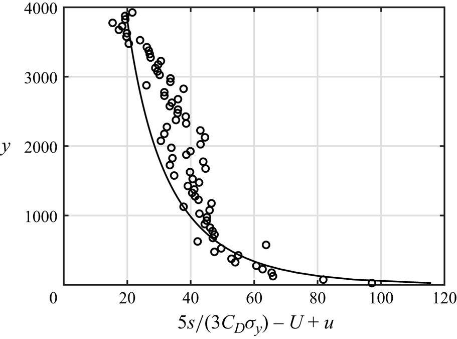
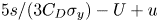
Appendix C. Boundary conditions for shallow impacts at a rigid, bumpy bed
For the case of a single angle of impact θ much less than  ${\rm \pi}$/2 of particles with a large coefficient of friction, so that rolling rather than sliding takes place, the negative of the average ratio of the vertical particle velocity after and before the impact is (Lämmel et al. Reference Lämmel, Dzikowski, Kroy, Oger and Valance2017)
 \begin{equation}\left\langle { - \frac{{\xi_{y,0}^ + }}{{\xi_{y,0}^ - }}} \right\rangle = - {e_t} + \frac{2}{3}({e_n} + {e_t})\sqrt {\frac{2}{\theta }\frac{{2{d_w}}}{{1 + {d_w}}}} ,\end{equation}
where en and et are the coefficients of normal and tangential restitution, respectively, and, here and in what follows, we use the subscript 0 to indicate quantities evaluated at the bed.
For saltation over a rigid, bumpy bed in viscous shearing flows, in the limit of large take-off velocity, (A8), (A12) and (2.24) give
 \begin{equation}\theta = \tan ( - \xi _{y,0}^ -{/}\xi _{x,0}^ - ) \simeq \frac{{{C_D}}}{{St(Sh - {s_0})}}.\end{equation}
In the case of saltation in turbulent shearing flows, instead, in the limit of large take-off velocity, (A8), (A19) and (2.37) give
 \begin{equation}\theta = \tan ( - \xi _{y,0}^ -{/}\xi _{x,0}^ - ) \simeq{-} {\left[ {{C_D}\frac{{\sqrt {r(Sh - {s_0})} }}{\kappa }\exp (C_D^2{y_0})Ei( - C_D^2{y_0})} \right]^{ - 1}}.\end{equation}
By inserting (A8) into (C1), we obtain
 \begin{equation}\langle \xi _{y,0}^ + \rangle = - \frac{{{e_t}}}{{{C_D}}} + \frac{{2\sqrt 2 }}{3}({e_n} + {e_t})\frac{1}{{{C_D}{\theta ^{1/2}}}}\sqrt {\frac{{2{d_w}}}{{1 + {d_w}}}} .\end{equation}
Then, we can assume that 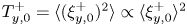 $T_{y,0}^ + = \langle {(\xi _{y,0}^ + )^2}\rangle \propto {\langle \xi _{y,0}^ + \rangle ^2}$, so that at leading order,
 \begin{equation}T_{y,0}^ + = {\alpha _T}\frac{1}{{C_D^2\theta }}\frac{{2{d_w}}}{{1 + {d_w}}},\end{equation}
with the coefficient of proportionality  ${\alpha _T}$ weakly dependent on the coefficients of normal and tangential restitution. Measurements in DC numerical simulations, with θ evaluated as the average angle of impact, shown in figure 15(a), confirm the validity of (C5), but indicate that the coefficient
  ${\alpha _T}$ also depends on the flow regime of the fluid. The reason is that the angle of impact is not actually unique: there is a distribution of impact angles of which either (C2) or (C3) provides the most likely value. Measurements in DC simulations (figure 16) reveal that the probability distributions of impact angles for saltation in viscous and turbulent shearing flows are indeed qualitatively different, with a tail respectively to the right or to the left of the peak.

Figure 15. Dependence of (a) the mean square of the vertical velocity of ascending particles at the bed and (b) the mean horizontal slip velocity on the mean impact angle measured in DC simulations of saltation in viscous (blue circles) and turbulent (orange diamonds) shearing flows. The lines are the predictions of (C5) and (C9), respectively, with:  ${\alpha _T} = 0.50$ and
  ${\alpha _u} = 0.60$ (blue solid lines);
  ${\alpha _T} = 0.18$ and
  ${\alpha _u} = 0.85$ (orange dashed lines). The drag coefficient is evaluated using (2.3a) for saltation in viscous flows, and (2.3b) for saltation in turbulent flows.

Figure 16. Examples of measured probability distribution function of impact angles in DC simulations of saltation in: (a) viscous and (b) turbulent shearing flows.
Lämmel et al. (Reference Lämmel, Dzikowski, Kroy, Oger and Valance2017) also obtained
 \begin{equation}\left\langle {\frac{{{{(\xi_{y,0}^ + )}^2} + {{(\xi_{x,0}^ + )}^2}}}{{{{(\xi_{y,0}^ - )}^2} + {{(\xi_{x,0}^ - )}^2}}}} \right\rangle = {\left[ {{e_t} - \frac{{(e_t^2 - e_n^2)}}{{2{e_t}}}\theta \frac{{2{d_w}}}{{1 + {d_w}}}} \right]^2},\end{equation}
so that, with (A8) and (A12), and  $\langle {(\xi _{x,0}^ + )^2}\rangle \propto {\langle \xi _{x,0}^ + \rangle ^2} = {\langle u_0^ + \rangle ^2}$,
 \begin{equation}u_0^ +\propto \sqrt {\frac{1}{{C_D^2}}\left( {1 + \frac{1}{{{\theta^2}}}} \right){{\left[ {{e_t} - \frac{{(e_t^2 - e_n^2)}}{{2{e_t}}}\theta \frac{{2{d_w}}}{{1 + {d_w}}}} \right]}^2} - T_{y,0}^ + } .\end{equation}
Then, we can determine the total particle slip velocity at the bed as
 \begin{equation}{u_0} = \frac{{c_0^ + u_0^ + + c_0^ - u_0^ - }}{{{c_0}}}.\end{equation}
With (B5) and (B6), and  $u_0^ -$ given by (A12), we obtain, at leading order,
 \begin{equation}{u_0} = {\alpha _u}\frac{1}{{{C_D}\theta }},\end{equation}
where, once again, the coefficient of proportionality  ${\alpha _u}$ is a weak function of the coefficients of restitution and the flow regime of the fluid (figure 15b). Using (C5) into (C9) gives
 \begin{equation}{u_0} = \frac{{{\alpha _u}}}{{{\alpha _T}}}\frac{{1 + {d_w}}}{{2{d_w}}}{C_D}T_{y,0}^ + .\end{equation}
It is worth mentioning that the values of  ${\alpha _u}$ that we employ do not exactly fit the dependence of the slip velocity on the impact angle (figure 15b), but do permit a satisfactory reproduction of the particle shear stress at the bed ((2.28) and (2.41)).
Appendix D. Discrete-continuum numerical simulations
The DC simulation is based on the combination of a DEM for the particle dynamics coupled to a continuum description of hydrodynamics, as developed in Durán et al. (Reference Durán, Andreotti and Claudin2012), Ralaiarisoa et al. (Reference Ralaiarisoa, Besnard, Furieri, Dupont, Ould El Moctar, Naaim-Bouvet and Valance2020) and Valance & Berzi (Reference Valance and Berzi2022).
The particle motion is described by a Lagrangian approach according to which the particle labelled p obeys the following dimensionless equations:
 \begin{gather}\frac{{\textrm{d}{\boldsymbol{\xi} ^p}}}{{\textrm{d}t}} = - {\boldsymbol{e}_y} + \sum\limits_q {\boldsymbol{f}_c^{p,q}} + \boldsymbol{f}_{drag}^p,\end{gather}
 \begin{gather}I\frac{{\textrm{d}{\boldsymbol{\omega }^p}}}{{\textrm{d}t}} = \frac{1}{2}\sum\limits_q {{\boldsymbol{n}^{p,q}}} \times \boldsymbol{f}_c^{p,q},\end{gather}
where  ${\boldsymbol{\xi }^p}$ and
  ${\boldsymbol{\omega }^p}$ are the translational and angular velocity vectors of particle p, respectively;
  ${\boldsymbol{e}_x}$ and
  ${\boldsymbol{e}_y}$ are the horizontal and vertical unit vectors, respectively;
  $\boldsymbol{f}_{drag}^p = {C_D}[(U - \xi _x^p){\boldsymbol{e}_x} - \xi _y^p{\boldsymbol{e}_y}]$ is the dimensionless drag force exerted by the fluid on the p-particle and
  $\boldsymbol{f}_c^{p,q}$ is the dimensionless contact force between particles p and q; I = 1/10 is the moment of inertia of a sphere; and
  ${\boldsymbol{n}^{p,q}}$ is the unit vector along the contact direction.
The normal component fc,n of the contact force is modelled by a linear spring dashpot, so that  ${f_{c,n}} = ({k_n}\delta + {\gamma _n}{v_n})$, where kn is the spring stiffness, δ the overlap between the compliant spheres, γn the viscous damping coefficient and vn the normal component of the relative translational particle velocities. The negative of the ratio between the normal relative velocity before and after the collision is the coefficient of normal restitution en. If the values of en and kn are prescribed, γn is deduced from the following relation:
  ${\gamma _n} = ({\rm \pi}/6)\sqrt {12{k_n}/(1 + {{\rm \pi}^2}/\ln {{({e_n})}^2})}$. The tangential component fc,t of the contact force is described via a Coulomb friction model regularized through a viscous damping:
  ${f_{c,t}} = - \min (\mu {f_{c,n}},{\gamma _t}{v_t})sign({v_t})$, where
  ${\rm \mu}$ is the Coulomb friction coefficient, vt the relative slip velocity at contact and γt the tangential viscous damping coefficient. The values chosen for the parameters are:
  ${k_n} = {\rm \pi}/6 \cdot {10^7}$,
  ${\gamma _n} = {\gamma _t},\;{e_n} = 0.88$ and
  ${\rm \mu}$ = 0.5.
The fluid motion is solved by an Eulerian description based on (2.24) or (2.37) for viscous and turbulent flows, respectively. The vertical component of the fluid velocity is assumed to be zero, so that only the horizontal momentum balance is required and reads
 \begin{equation}\frac{{\textrm{d}S}}{{\textrm{d}y}} = {F_x},\end{equation}
where  ${F_x} = c\langle \sum\nolimits_{p \in [y;y + \textrm{d}y]} {{C_D}(U - {\xi _x})} \rangle /\langle \sum\nolimits_{p \in [y;y + \textrm{d}y]} 1 \rangle$, with the angular brackets denoting ensemble averaging, represents the x-component of the average volume force exerted on the fluid by the particles whose centres are located in the horizontal slice between y and y + dy. The integration of (D3) gives
 \begin{equation}S = Sh - \int_0^\infty {{F_x}\,\textrm{d}y} ,\end{equation}
where the infinite upper bound of the integral means that all moving grains located above y must be accounted for. Once the vertical profile S(y) of the fluid shear stress is determined, the horizontal fluid velocity profile can then be obtained from the integration equation (2.24) or (2.37) for viscous and turbulent shearing flows, respectively, with the no-slip boundary condition U = 0 at y = 0.
The simulated system is quasi-two-dimensional with a streamwise length equal to 5120 particle diameters and a transverse length equal to one diameter. We use spherical particles with a polydispersity of ±10 % and adjust their number in the system to obtain the desired value of the particle hold-up M. Periodic boundary conditions are employed in the streamwise direction. The domain is not upper bounded, while the lower boundary is composed of a layer of immobile particles of diameter dw in close contact (rigid, bumpy bed; see figure 1). As mentioned earlier in the paper, we suppress the possibility of particle–particle collisions above the bed.
Operatively, at every time step, we integrate equations (D1) and (D2) for every particle in the system and determine its new velocity and position. We then use this information to update the profiles of fluid shear stress and horizontal velocity via (2.4), and (2.24) for viscous flows or (2.37) for turbulent flows and proceed with the next time step until we reach a steady state, that is, when the horizontal mass flux averaged over a window of 100 unit time steps is stationary. Initially, the fluid profile is taken to be linear or logarithmic for viscous and turbulent shearing flows, respectively, and corresponds to the unperturbed profile in the absence of particles. The particles are initially displayed on a horizontal row located at ten diameters from the rigid, bumpy bed, with a constant inter-particle distance equal to two diameters and zero initial velocity. Importantly, the final state is independent of the initial conditions as long as the number of particles in the flow does not surpass its transport capacity.
As mentioned, we have suppressed the possibility of mid-trajectory particle–particle interactions in the numerical simulations. However, we have also carried out simulations that incorporate mid-trajectory collisions. As shown in figure 17, such collisions begin to influence the particle flux only for large particle hold-ups, with a concentration that results in a mean free path that does not satisfy the condition of (2.23).

Figure 17. Particle flux against particle hold-up measured in DC numerical simulations with (orange diamonds) and without (blue diamonds) mid-trajectory collisions, in the case of saltation in turbulent shearing flows with dw = 1.5, St = 1681, r = 2208 and Sh = 0.04.


