2. Existing methods

2.1. Linear equality constraints

Constraints where the decision variables ${\boldsymbol x}$ appear only linearly can be handled efficiently by suitably redefining variables. A problem with linear constraints can be written as

(2.1)\begin{equation} \left.\begin{array}{cl@{}} \displaystyle \min_{{\boldsymbol x} \in R^n} & f({\boldsymbol x}) \\ \textrm{s.t.} & A {\boldsymbol x} - {\boldsymbol b} = 0 \\ \end{array}\right\}, \end{equation}

where $A \in R^{m \times n}$ and ${\boldsymbol b} \in R^m$, $m \le n$ are the coefficients that define the linear constraint. We can then decompose ${\boldsymbol x} = {\boldsymbol x}_p + Z {\boldsymbol y}$ where ${\boldsymbol x}_p \in R^n$ is any particular solution to the underdetermined system $A {\boldsymbol x} = {\boldsymbol b}$ (typically taken to be the least-norm solution), $Z \in R^{n \times (n-m)}$ is a (typically orthogonal) representation for the null space of $A$, such that $AZ=0$, and ${\boldsymbol y} \in R^{n-m}$ is an arbitrary vector. This allows us to write the problem as

(2.2)\begin{equation} \min_{{\boldsymbol y} \in R^{n-m}} \quad f({\boldsymbol x}_p + Z{\boldsymbol y}), \end{equation}

which is now an unconstrained problem, where any value for ${\boldsymbol y}$ is feasible, and the full solution ${\boldsymbol x}^*$ can be recovered as ${\boldsymbol x}_p + Z {\boldsymbol y}^*$.

While simple to deal with, linear equality constraints are very limited in their applicability. Most constraints that are of interest in stellarator optimization are nonlinear, making linear equality constraints only useful for enforcing simple boundary conditions on the plasma boundary and profiles.

2.2. Sum of squares

Perhaps the simplest way to (approximately) solve (1.3) is with a quadratic penalty method, where the objective and constraints are combined into a single function, which is then minimized without constraints:

(2.3)\begin{equation} \min_{\boldsymbol x} \quad f({\boldsymbol x}) + w_1 \| {\boldsymbol g}({\boldsymbol x}) \|^2 + w_2 \| I_{({\boldsymbol l},{\boldsymbol u})}({\boldsymbol x}) \|^2.\end{equation}

Here $w_1$ and $w_2$ are weights and $I_{(l,u)}({\boldsymbol x})$ is a ‘deadzone’ function:

(2.4)\begin{equation} I_{({\boldsymbol l},{\boldsymbol u})}({\boldsymbol x}) = \left\{ \begin{array}{@{}cc@{}} 0 & \text{if } {\boldsymbol l} \le {\boldsymbol x} \le {\boldsymbol u} \\ \max ({\boldsymbol x}-{\boldsymbol u}, {\boldsymbol l}-{\boldsymbol x}) & \text{otherwise} \end{array}\right\}. \end{equation}

This formulation is used by a number of codes for optimizing stellarator equilibria, such as SIMSOPT, STELLOPT, ROSE and DESC. Similar techniques have also been used for coil design in FOCUS (Kruger et al. Reference Kruger, Zhu, Bader, Anderson and Singh2021). While simple to implement, this formulation has a number of drawbacks.

1. (i) The weights $w$ must be determined by the user, often through extensive trial and error. This can be automated by iteratively increasing the weights until the constraint violation is reduced to an acceptable level, as in Bindel, Landreman & Padidar (Reference Bindel, Landreman and Padidar2023), though this leads to the next problem.

2. (ii) Formally, the constraints are only satisfied as $w \rightarrow \infty$ and reducing constraint violation to an acceptable level can often require very large values of the weights, leading to a badly scaled problem that can slow convergence.

3. (iii) The $\max$ term in the deadzone function introduces a discontinuity in the second derivative of the objective, which can hinder progress of some optimization methods that assume the objective and constraints to be at least C2. This can be partially alleviated by using a quartic or exponential penalty instead of quadratic, as in Kruger et al. (Reference Kruger, Zhu, Bader, Anderson and Singh2021), though this makes the problem more nonlinear and can reduce the efficiency of many optimizers that assume a locally linear or quadratic model function.

2.3. Projection methods

The constraint of MHD equilibrium is most commonly dealt with by using a fixed boundary equilibrium solver at each step in the optimization. Given the plasma boundary and profiles at the latest optimization step, the equilibrium solver is run to determine the full solution throughout the plasma volume, and this is then used to evaluate the objective function. This is akin to a projection method, where after each step of the optimizer, the solution is projected back onto the feasible region $\{{\boldsymbol x} \mid {\boldsymbol g}({\boldsymbol x})=0\}$. This also suffers from a number of drawbacks.

1. (i) The equilibrium must be resolved at each step of the optimizer, possibly multiple times if finite differences are used to evaluate derivatives. This can be made somewhat more efficient if a warm start is used based on the previous accepted step (Conlin et al. Reference Conlin, Dudt, Panici and Kolemen2023; Dudt et al. Reference Dudt, Conlin, Panici and Kolemen2023), though this is still often the most expensive part of the optimization loop.

2. (ii) Projection type methods are limited in applicability to constraints for which a projection operator can be defined. The MHD equilibrium solvers can serve this function for equilibrium constraints, but a projection operator for a general nonlinear constraint is not known.

3. (iii) Enforcing that the constraints are satisfied at each step of the optimization may be too strict and cause the optimizer to stop at a poor local minimum.

This last point is illustrated in figure 1. Points where the constraint curve $g({\boldsymbol x})=0$ is tangent to the contours of $f$ are local minima of the constrained problem, where following the constraint curve will lead to higher objective function values, but moving in a direction to decrease the objective function will violate the constraints. If we enforce that the constraint is satisfied at each step, we will follow the path in red and stop at the local minimum $x_1$. However, if we are allowed to temporarily violate the constraints, we can make rapid progress towards the better local minimum $x_2$.

Figure 1. Sketch of optimization landscape (contours of $f$ in blue) with constraints (curve of $g(x)=0$ in black). Starting from $x_0$ and enforcing the constraints exactly at each step will follow the red path and end at $x_1$. If we allow ourselves to temporarily violate the constraints, we can follow the green path and arrive at the better solution $x_2$.

Some may worry that not enforcing MHD equilibrium at each step may lead the optimizer in directions that are not dynamically accessible during an actual plasma discharge, where the plasma is assumed to be in equilibrium; however, it is important to note that the path taken through phase space during optimization in general has no connection to the path taken during an actual discharge, and just because the optimizer finds a path that violates equilibrium does not mean there is not a nearby path that satisfies it. Dynamical accessibility is an important aspect of stellarator optimization, but the expense of time-dependent simulations preclude their use inside an optimization loop, so are generally limited to post-optimization validation and analysis.

3. Methods for constrained optimization

We consider a general constrained optimization problem of the form

(3.1)\begin{equation} \left.\begin{array}{cl@{}} \displaystyle \min_{\boldsymbol x} & f({\boldsymbol x}) \\ \textrm{s.t.} & {\boldsymbol g}_E({\boldsymbol x}) = 0 \\ & {\boldsymbol g}_I({\boldsymbol x}) \ge 0 \\ \end{array}\right\}, \end{equation}

where, as before, ${\boldsymbol g}_E$ and ${\boldsymbol g}_I$ denote the equality and inequality constraints, respectively. Most analysis and algorithms start from the Lagrangian for this problem, which is

(3.2)\begin{equation} \mathcal{L}({\boldsymbol x}, {\boldsymbol y}_E, {\boldsymbol y}_I) = f({\boldsymbol x}) - {\boldsymbol y}_E^T {\boldsymbol g}_E({\boldsymbol x}) - {\boldsymbol y}_I^T {\boldsymbol g}_I({\boldsymbol x}), \end{equation}

where ${\boldsymbol y}_E$ and ${\boldsymbol y}_I$ are the Lagrange multipliers associated with the equality and inequality constraints, respectively. The conditions for a given set $({\boldsymbol x}^*, {\boldsymbol y}_E^*, {\boldsymbol y}_I^*)$ to be a solution to (3.1) are the so called Karush–Kuhn–Tucker (KKT) conditions (Nocedal & Wright Reference Nocedal and Wright2006):

(3.3a)\begin{gather} \nabla_{\boldsymbol x} \mathcal{L}({\boldsymbol x}^*, {\boldsymbol y}_E^*, {\boldsymbol y}_I^*) = \boldsymbol{\nabla} f - {\boldsymbol y}_E^T \boldsymbol{\nabla} {\boldsymbol g}_E - {\boldsymbol y}_I^T \boldsymbol{\nabla} {\boldsymbol g}_I = 0, \end{gather}

(3.3b)\begin{gather}{\boldsymbol g}_E({\boldsymbol x}^*) = 0, \end{gather}

(3.3c)\begin{gather}{\boldsymbol g}_I({\boldsymbol x}^*) \geq 0, \end{gather}

(3.3d)\begin{gather}{\boldsymbol y}_I^* \geq 0 , \end{gather}

(3.3e)\begin{gather}{\boldsymbol y}_E^* \boldsymbol{\cdot} {\boldsymbol g}_E({\boldsymbol x}^*) = 0, \end{gather}

(3.3f)\begin{gather}{\boldsymbol y}_I^* \boldsymbol{\cdot} {\boldsymbol g}_I({\boldsymbol x}^*) =0. \end{gather}

The first condition is reminiscent of the first-order optimality condition for an unconstrained problem, $\boldsymbol {\nabla } f({\boldsymbol x}^*) = 0$, with the objective function $f$ replaced by the Lagrangian $\mathcal {L}$; however, it is important to note that we do not seek a minimum of the Lagrangian. It can be shown that solutions to (3.3) always lie at a saddle point where the Lagrangian is minimized with respect to the primal variables ${\boldsymbol x}$ and maximized with respect to the dual variables ${\boldsymbol y}$.

It is useful to take a moment to consider the meaning and utility of the Lagrange multipliers ${\boldsymbol y}$. A first insight into the meaning of Lagrange multipliers can be found from the last of the KKT conditions in (3.3f), i.e.

(3.4)\begin{equation} {\boldsymbol y}_I^* \boldsymbol{\cdot} {\boldsymbol g}_I({\boldsymbol x}^*) = 0, \end{equation}

meaning that either the constraint is zero or its associated multiplier is zero for each constraint. For a problem in the form of (3.1), an inequality constraint not equal to zero is said to be ‘non-binding’ or ‘not active’, meaning that the constraint has no effect on the solution, and the minimum would not change if the constraint were removed. This is contrasted with a ‘binding’ or ‘active’ constraint that is preventing the solution from improving the objective $f$. This suggests that the Lagrange multipliers contain information about how much the constraints are affecting the solution. This can be made more explicit by considering the following problem:

(3.5)\begin{equation} \left.\begin{array}{cl@{}} \displaystyle \min_{\boldsymbol x} & f(x) \\ \textrm{s.t.} & g(x) = 0 \\ \end{array}\right\}. \end{equation}

The Lagrangian for this problem is

(3.6)\begin{equation} \mathcal{L}(x,y) = f(x) - y g(x). \end{equation}

We can now consider what happens if we perturb the constraint $g = 0$ to $g + \delta g = 0$.

From (3.3a) we see that at an optimum $x^*$ the change in the Lagrangian must be zero to first order, which gives

(3.7)\begin{equation} \delta f = y \delta g. \end{equation}

Here we see that the Lagrange multipliers tell us how much our objective can improve by relaxing our constraints, or the so called ‘marginal cost’ of enforcing the constraint $g = 0$. Additionally, the sign of the multipliers tells us which direction we should relax the constraints to improve the objective.

We can use a similar approach to consider trade offs between conflicting constraints, where if we have constraints $g_1$ and $g_2$ that cannot both be satisfied, the ratio of their multipliers $y_1/y_2$ tells us how much we can expect to improve $g_1$ by relaxing $g_2$ and vice versa.

A number of methods have been developed for solving constrained optimization problems, which we briefly summarize in the following subsections. More information can be found in standard texts on numerical optimization (Conn, Gould & Philippe Reference Conn, Gould and Philippe2000; Nocedal & Wright Reference Nocedal and Wright2006)

3.1. Interior point methods

A popular class of methods for dealing with inequality constraints are the so-called ‘interior point’ methods, or sometimes referred to as ‘log barrier’ methods. These methods solve problems of the form

(3.8)\begin{equation} \left.\begin{array}{cl@{}} \displaystyle \min_{\boldsymbol x} & f({\boldsymbol x}) \\ \textrm{s.t.} & {\boldsymbol g}({\boldsymbol x}) = 0 \\ & 0 \le {\boldsymbol x} \\ \end{array}\right\}, \end{equation}

(any problem of the form of (1.3) can be transformed into this form by appropriate change of variables). The bound on the variables is replaced by a logarithmic penalty term:

(3.9)\begin{equation} \left.\begin{array}{cl@{}} \displaystyle \min_{\boldsymbol x} & \displaystyle f({\boldsymbol x}) - \mu \sum_i \log{x_i} \\ \textrm{s.t.} & {\boldsymbol g}({\boldsymbol x}) = 0 \\ \end{array}\right\}. \end{equation}

This problem is then solved repeatedly with an equality constrained optimization method such as sequential quadratic programming (SQP, see the following section) for a decreasing sequence of barrier parameters $\mu$. For finite values of $\mu$, the log term pushes the solution into the interior of the feasible set (hence the name), and the solution is allowed to approach the boundary as the barrier gets sharper as $\mu$ approaches zero.

The interior point method is the basis of a number of popular commercial and open-source optimization codes (Wächter & Biegler Reference Wächter and Biegler2006; Biegler & Zavala Reference Biegler and Zavala2009), but we have found that in practice they do not perform well on the types of problems commonly encountered in stellarator optimization, for reasons that will be discussed further in § 4

3.2. Sequential quadratic programming methods

Another popular class of methods are based on sequentially minimizing an approximate model of the objective and constraints. Typically, the objective is modelled as quadratic and the constraints are modelled as linear, leading to a standard quadratic program. If the current estimate of the solution is ${\boldsymbol x}_k$, we seek the next iterate ${\boldsymbol x}_{k+1} = {\boldsymbol x}_k + {\boldsymbol p}$ by solving the following subproblem:

(3.10)\begin{equation} \left.\begin{array}{c@{}} \begin{aligned} \min_{\boldsymbol p} \quad & {\boldsymbol p}^T H {\boldsymbol p} + {\boldsymbol g}^T {\boldsymbol p} \\ \textrm{s.t.} \quad & A_E {\boldsymbol p} ={-}{\boldsymbol g}_E({\boldsymbol x}_k) \end{aligned}\\ {\boldsymbol l} - {\boldsymbol g}_I({\boldsymbol x}_k) \le A_I {\boldsymbol p} \le {\boldsymbol u} - {\boldsymbol g}_I({\boldsymbol x}_k) \end{array}\right\}. \end{equation}

Here ${\boldsymbol g}$ and $H$ are the gradient and Hessian of $f$ and $A_E$, and $A_I$ are the Jacobian matrices of the equality and inequality constraints ${\boldsymbol g}_E$ and ${\boldsymbol g}_I$.

One common issue with SQP methods is the possible inconsistency of the linearized constraints, such that the subproblem (3.10) has no solution. This problem can be made worse by the inclusion of a trust region constraint, as is often used to ensure global convergence. To overcome this, the full step ${\boldsymbol p}$ is typically broken into two sub-steps, one of which attempts to achieve feasibility with respect to the linearized constraints as much as possible, while the other attempts to reduce the objective function. A merit function is then used to balance between improving the objective and decreasing the constraint violation (Conn et al. Reference Conn, Gould and Philippe2000).

Similar to interior point methods, SQP methods form the core of a number of commercial and open-source optimization codes (Gill, Murray & Saunders Reference Gill, Murray and Saunders2005; Johnson & Schueller Reference Johnson and Schueller2021). However, we similarly see that the performance of existing implementations is limited on the types of problems encountered in practice.

3.4. Augmented Lagrangian methods

For the quadratic penalty method considered in (2.3), one can show that the constraint violation is inversely proportional to the penalty parameter

(3.11)\begin{equation} g_i({\boldsymbol x}_k) \approx{-}y_i^* /\mu_k, \end{equation}

where $y_i^*$ is the true Lagrange multiplier (from the solution to (3.3)) associated with the constraint $g_i$ and $\mu _k$ is the penalty parameter. We see that if we want to satisfy the constraints exactly, we must have $\mu \rightarrow \infty$, which as discussed can be numerically intractable. However, if we consider the ‘augmented’ Lagrangian

(3.12)\begin{equation} \mathcal{L}_A({\boldsymbol x}, {\boldsymbol y}, \mu) = f({\boldsymbol x}) - {\boldsymbol y}^T {\boldsymbol g}({\boldsymbol x}) + \frac{\mu}{2} \| {\boldsymbol g}({\boldsymbol x})\|^2, \end{equation}

where ${\boldsymbol y}$ are estimates of the true Lagrange multipliers, one can show that now (Nocedal & Wright Reference Nocedal and Wright2006)

(3.13)\begin{equation} g_i({\boldsymbol x}_k) \approx{-}(y_i^* - y_i^k) /\mu_k. \end{equation}

So that if our estimate of the true Lagrange multipliers is accurate, we can significantly reduce the constraint violation without requiring the penalty parameter to grow without bound. This also gives us a rule to update our estimate of the multipliers:

(3.14)\begin{equation} y_i^{k+1} = y_i^k - \mu_k g_i({\boldsymbol x}_k). \end{equation}

Minimizing the augmented Lagrangian with fixed ${\boldsymbol y}$ and $\mu$ is an unconstrained or bound constrained problem, for which standard gradient or Newton-based methods can be used. From this solution we obtain an approximation to the true solution of the constrained problem. We can then update the multipliers and penalty term and re-optimize, eventually converging to the true solution. This is the basic method used in several widely used codes (Conn, Gould & Toint Reference Conn, Gould and Toint2013; Fowkes et al. Reference Fowkes2023) and can also be used as a generic technique to handle constraints for algorithms that otherwise would only be able to solve unconstrained problems (Johnson & Schueller Reference Johnson and Schueller2021).

One can also construct an augmented Lagrangian for a least squares problem. Because $L({\boldsymbol x}, {\boldsymbol y}, \mu )$ is only ever minimized with respect to ${\boldsymbol x}$, one can add any quantity independent of ${\boldsymbol x}$ without affecting the result. In particular, if we add $\| {\boldsymbol y}\|^2/2\mu$, we get

(3.15)\begin{equation} \mathcal{L}_A({\boldsymbol x}, {\boldsymbol y}, \mu) = \tfrac{1}{2} \| {\boldsymbol f}({\boldsymbol x})\|^2 - {\boldsymbol y}^T {\boldsymbol g}({\boldsymbol x}) + \mu/2 \| {\boldsymbol g}({\boldsymbol x})\|^2 + \| {\boldsymbol y}\|^2/2\mu. \end{equation}

We can then complete the square to obtain

(3.16)\begin{equation} \mathcal{L}_A({\boldsymbol x}, {\boldsymbol y}, \mu) = \tfrac{1}{2} \| {\boldsymbol f}({\boldsymbol x})\|^2 + \tfrac{1}{2} \| -{\boldsymbol y}/\sqrt{\mu} + \sqrt{\mu}{\boldsymbol g}({\boldsymbol x})\|^2.\end{equation}

This allows us to use standard unconstrained or bound constrained least squares routines to solve the augmented Lagrangian subproblem, which has a number of benefits.

1. (i) Super-linear convergence can be obtained using only first derivatives of ${\boldsymbol f}$ and ${\boldsymbol g}$ (provided the residual is sufficiently small at the solution, which in practice is very often the case) as opposed to standard Newton methods that require second derivatives of the objective and constraints.

2. (ii) The quadratic subproblem that arises in least squares is always convex, for which the exact solution can be found efficiently.

These benefits can also be obtained using other quasi-Newton methods such as BFGS, which also require only first derivatives and have convex subproblems, but in practice we have found that in the common case where the problem has a natural least squares structure, using a least squares method significantly outperforms BFGS in both time and number of iterations required to reach a solution.

4. Constrained optimization in DESC

As previously mentioned there are a wide variety of commercial and open-source codes for constrained optimization, many of which have been interfaced to the DESC stellarator optimization code (Dudt & Kolemen Reference Dudt and Kolemen2020; Conlin et al. Reference Conlin, Dudt, Panici and Kolemen2023; Dudt et al. Reference Dudt, Conlin, Panici and Kolemen2023, Reference Dudt, Conlin, Panici, Kolemen, Unalmis and Kim2024; Panici et al. Reference Panici, Conlin, Dudt, Unalmis and Kolemen2023). In practice, we have found that most of the existing methods perform somewhat poorly on the types of problems encountered in stellarator optimization. We hypothesize this is for a number of reasons.

1. (i) Many commercial solvers assume a particular structure for the problem, such as quadratic, conic and semi-definite programming solvers. Others rely on convexity, partial separability or other conditions that generally do not hold in stellarator optimization.

2. (ii) Many codes are designed and optimized for solving very-high-dimensional problems ($O(10^6)$ variables or more) but with a high degree of sparsity, and make extensive use of sparse and iterative linear algebra methods. In stellarator optimization problems we generally do not have significant sparsity due to the wide use of spectral methods, making these methods inefficient.

3. (iii) The types of problems in stellarator optimization are often poorly scaled, due to a wide range of scales in physical units, and due to spectral discretizations. This can lead to failure of iterative linear algebra subproblems without a proper preconditioner (which may not be easy to determine) and can also slow progress of the overall optimization because the optimization landscape is strongly anisotropic (meaning the objective is much more sensitive to changes in certain directions in parameter space than others, such as a long narrow valley).

4. (iv) No existing implementations that we are aware of take advantage of graphics processing unit (GPU) acceleration for the underlying linear algebra. This is partially by design, as GPUs are often of little benefit for the types of large sparse problems existing codes are designed for. However, as previously mentioned, the problems in stellarator optimization tend to be moderately sized and dense, for which GPU linear algebra can provide a significant benefit.

Because of this, we have implemented a new optimizer based on the least squares augmented Lagrangian formalism from § 3.4, and a sketch of the algorithm is found in algorithm 1. Future work could include re-implementations of SQP or interior point methods to better handle dense and poorly scaled linear systems as these methods can be very powerful, though existing implementations do not seem to perform well.

Before applying the augmented Lagrangian method, we first transform any inequality constraints into equality constraints plus bounds using slack variables as in (1.3). The augmented Lagrangian is then used to handle the equality constraints, while the bound constraints are handled by using a Coleman–Li type trust region method (Coleman & Li Reference Coleman and Li1996) where the trust region is adjusted at each iteration to account for the bounds, ensuring that iterates remain strictly feasible with respect to the bound constraints.

Algorithm 1 Augmented Lagrangian algorithm (adapted from Conn et al. Reference Conn, Gould and Philippe2000; Nocedal & Wright Reference Nocedal and Wright2006)

The precise rules for updating the tolerances and penalty parameters can be varied, see (Conn et al. Reference Conn, Gould and Philippe2000) for a more complex version, though we have found that in practice the results and performance do not significantly depend on the choice of hyperparameters. These rules are effectively automatically finding the correct weights to manage the trade-off between improving the objective value and constraint feasibility that would normally require extensive user trial and error.

5. Examples

Many optimized stellarators have very strongly shaped boundaries, and a ‘bean’ shaped cross-section is quite common, appearing in designs such as NCSX (shown in figure 2), W7-X, ARIES-CS and many recent designs such as the ‘precise’ quasi-symmetric equilibria of Landreman and Paul (Landreman & Paul Reference Landreman and Paul2022). These strongly indented shapes can be difficult to create with external coils or magnets, often requiring coils that are very close on the inboard concave side (Landreman & Boozer Reference Landreman and Boozer2016; Kappel, Landreman & Malhotra Reference Kappel, Landreman and Malhotra2024).

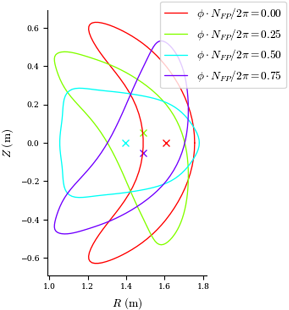
Figure 2. Plasma boundary of NCSX at several cross-sections, with the ‘bean’ section at $\phi =0$.

We can attempt to alleviate this problem with constrained optimization by properly constraining the curvature of the surface. We consider a surface parameterized by the poloidal angle $\theta$ and toroidal angle $\zeta$, with parameterization ${\boldsymbol r}(\theta, \zeta )$. The covariant basis vectors are given by ${\boldsymbol r}_\alpha (\theta, \zeta ) = \partial _\alpha {\boldsymbol r}(\theta, \zeta )$ for $\alpha \in (\theta, \zeta )$. From these we can construct the ‘first fundamental form’ as (Do Carmo Reference Do Carmo2016)

(5.1)\begin{equation} \mathcal{F} = \begin{pmatrix} E & F \\ F & G \\ \end{pmatrix}, \end{equation}

where the coefficients are dot products of the first derivative of the position vector:

(5.2)\begin{gather} E = {\boldsymbol r}_\theta \boldsymbol{\cdot} {\boldsymbol r}_\theta, \end{gather}

(5.3)\begin{gather}F = {\boldsymbol r}_\theta \boldsymbol{\cdot} {\boldsymbol r}_\zeta , \end{gather}

(5.4)\begin{gather}G = {\boldsymbol r}_\zeta \boldsymbol{\cdot} {\boldsymbol r}_\zeta . \end{gather}

Similarly, we can define the ‘second fundamental form’ as

(5.5)\begin{equation} \mathcal{S} = \begin{pmatrix} L & M \\ M & N \\ \end{pmatrix}, \end{equation}

where the coefficients are given by the projection of the second derivatives of the position vector onto the surface normal:

(5.6)\begin{gather} L = {\boldsymbol r}_{\theta \theta} \boldsymbol{\cdot} {\boldsymbol n}, \end{gather}

(5.7)\begin{gather}M = {\boldsymbol r}_{\theta \zeta} \boldsymbol{\cdot} {\boldsymbol n}, \end{gather}

(5.8)\begin{gather}N = {\boldsymbol r}_{\zeta \zeta} \boldsymbol{\cdot} {\boldsymbol n}. \end{gather}

We can then compute the principal curvatures $\kappa _1$ and $\kappa _2$ of the surface as the solutions to the generalized eigenvalue problem

(5.9)\begin{equation} \mathcal{S}{\boldsymbol u} = \kappa \mathcal{F} {\boldsymbol u}, \end{equation}

where the eigenvectors ${\boldsymbol u}$ are called the principal directions. The principal curvatures are the maximum and minimum of the inverse radii of curvature of all the curves that are tangent to the surface at a given point, with the sign convention that positive curvature means the surface curves towards the normal vector.

On the inboard side of a toroidal surface, we expect at least one of the principal curvatures to be positive because the surface curves towards the normal in the toroidal direction, while at least one should be negative on the outboard side. Indenting of the poloidal cross-section characteristic of the bean shape would manifest as both principal curvatures being positive on the inboard side and both negative on the outboard side.

To prevent strong indentation, we use the mean curvature, defined as $H = 1/2(\kappa _1 + \kappa _2)$, and enforce that the mean curvature is everywhere negative. On the outboard side, where both curvatures are already negative this should have minimal effect, while on the inboard it forces any indent to have a larger radius of curvature than the local major radius.

In addition to this constraint on the curvature of the plasma surface, we also include constraints to enforce MHD equilibrium, fix the major radius $R_0$, aspect ratio $R_0/a$, total enclosed volume $V$ (which we fix equal to the volume of the initial guess, a circular torus) and include inequality constraints on the rotational transform profile $\iota$. We also fix the profiles of pressure $p$ and current $j$ and the total enclosed flux $\varPsi$ to give an average field strength of 1 T. In summary, our constraints are

(5.10)\begin{equation} \left.\begin{array}{c@{}} R_0 = 1\ \mathrm{m} \\ R_0/a = 6 \\ V = V_{init} \sim 0.55\ \mathrm{m}^3 \\ 0.43 < \iota(\rho) < 0.5 \\ H(\theta, \zeta) < 0\ \mathrm{m}^{{-}1}\\ p(\rho) = 0\ \mathrm{Pa} \\ j(\rho) = 0\ \mathrm{A} \\ \varPsi = 0.087\ \mathrm{Tm}^2 \\ {\boldsymbol J} \times {\boldsymbol B} - \boldsymbol{\nabla} p = 0 \\ \end{array}\right\}. \end{equation}

As our objective, we use the ‘two-term’ metric $f_C$ for quasi-symmetry (Isaev, Mikhailov & Shafranov Reference Isaev, Mikhailov and Shafranov1994; Rodriguez, Paul & Bhattacharjee Reference Rodriguez, Paul and Bhattacharjee2022; Dudt et al. Reference Dudt, Conlin, Panici and Kolemen2023), targeting quasi-axisymmetry at 10 surfaces evenly spaced throughout the volume. The quasi-symmetry metric $f_C$ is given by

(5.11)\begin{equation} f_C = (M \iota - N) ({\boldsymbol B} \times \boldsymbol{\nabla} \psi) \boldsymbol{\cdot} \boldsymbol{\nabla} B - (M G + N I) {\boldsymbol B} \boldsymbol{\cdot} \boldsymbol{\nabla} B. \end{equation}

Here, ${\boldsymbol B}$ is the magnetic field with magnitude $B$, $M$ and $N$ give the type of quasi-symmetry (for quasi-axisymmetric, $M=1$, $N=0$), and $G$ and $I$ are the poloidal and toroidal covariant components of the field in Boozer coordinates.

The plasma boundary after optimization is shown in figure 3, and we can see that we have successfully avoided any concave regions that may be difficult to produce with external coils. In figure 6 we also see that the level of quasi-symmetry in this new configuration compares quite well with similar optimized designs such as NCSX. However, upon further analysis we find that this new configuration has a negative magnetic well, indicating it is MHD unstable.

Figure 3. Plasma boundary of new optimized configuration with constraint on surface curvature.

We can attempt to rectify this by adding a constraint on the magnetic well shown in (5.12). Here $V(\rho )$ is the volume enclosed by the flux surface labelled by $\rho$ and $\langle \cdots \rangle$ is a flux surface average. For vacuum equilibria, this is physically equivalent to the more common metric $V''(\psi ) < 0$ but generalizes to finite beta as well (Landreman & Jorge Reference Landreman and Jorge2020). The constraint is enforced at 20 surfaces evenly spaced in $\rho$. The definition for magnetic well used is

(5.12)\begin{equation} W(\rho) = \frac{V}{\langle B^2 \rangle \partial_\rho V} \partial_\rho \langle 2\mu_0 p + B^2 \rangle > 0. \end{equation}

Adding this constraint and re-running the optimization, we find that the optimizer does not converge, indicating that the constraints cannot all be satisfied at the same time. This is perhaps expected, as empirical evidence suggests that bean-like cross-sections can be favourable for MHD stability (Nührenberg & Zille Reference Nührenberg and Zille1986; Nührenberg Reference Nührenberg2010), though may not be strictly required from a near axis formalism (Rodríguez Reference Rodríguez2023).

However, in this case we can use the estimated Lagrange multipliers to get an idea of which constraints are the most limiting. Because the curvature constraint is enforced pointwise in real space, the Lagrange multipliers also have a local characteristic, and we can plot them over the surface to see where the optimizer would indent the surface, as shown in figure 4. As expected, the curvature constraint is most prominent on the inboard side, and the negative sign of the multipliers indicates that increasing the curvature in those regions will be favourable for stability.

Figure 4. Lagrange multipliers for the curvature constraint plotted on the surface. The dark areas indicate places where the constraint is binding, and the optimizer wants to indent the boundary in those locations to improve the magnetic well.

Using this information, we re-run the optimization with the magnetic well constraint, but reduce the upper bound on mean curvature from 0 m$^{-1}$ to 0.5 m$^{-1}$. With this relaxed constraint we are able to achieve a stable magnetic well, while maintaining most of the benefits of the curvature constraint, as shown in figure 5. This is not without some cost, as we see in figure 6 that the level of quasi-symmetry for the stable configuration is degraded somewhat compared with the unstable one, though still at reasonable levels compared with other optimized configurations such as NCSX.

Figure 5. Plasma boundary of new optimized configuration with relaxed curvature constraint and stable magnetic well.

Figure 6. Quasi-symmetry error measured by the maximum amplitude of the symmetry breaking Boozer harmonics for the newly optimized configuration with and without a magnetic well constraint, compared with NCSX.