


1. Introduction
Turbulent transport is known to determine the energy confinement time of fusion devices. Quantifying, predicting and controlling this turbulent transport is a prerequisite for designing optimized fusion power plants and is therefore considered a key open problem in fusion research. While high-fidelity numerical simulations based on first principles are crucial for understanding the complex mechanisms behind turbulent transport, they are often computationally too expensive for routine use in tasks like optimization or uncertainty quantification that involve large ensembles of simulations. Constructing computationally cheap yet reliable surrogate models is therefore highly desirable in practice.
In Farcaş, Merlo & Jenko (Reference Farcaş, Merlo and Jenko2022), we proposed a sensitivity-driven dimension-adaptive sparse grid framework for uncertainty quantification (UQ) and sensitivity analysis (SA) at scale, which was applied to the problem of turbulent transport in the pedestal region of a tokamak driven by electron temperature gradient (ETG) modes. The sensitivity-driven approach intrinsically provides an interpolation-based surrogate model, which turned out to provide accurate predictions for the scenario studied in Farcaş et al. (Reference Farcaş, Merlo and Jenko2022) for testing parameters within the interpolation bounds. However, since polynomial extrapolation is, in general, ill posed and unstable (Trefethen Reference Trefethen2012), we will not use this model for predictions outside the interpolation bounds used for its construction. In addition, this interpolation model does not incorporate a quantification of prediction uncertainty, which is crucial for assessing the trustworthiness of surrogate transport models for any given input parameters. The present paper builds on Farcaş et al. (Reference Farcaş, Merlo and Jenko2022) and leverages the aforementioned sensitivity-driven approach to derive a generic and parsimonious surrogate transport model for ETG-driven turbulent fluxes that (i) depends on physically interpretable parameters, (ii) generalizes beyond training and, importantly, (iii) incorporates a quantification of prediction uncertainty.
Electron temperature gradient turbulence has been the subject of theoretical and numerical investigations for more than two decades, from the seminal works by Jenko et al. (Reference Jenko, Dorland, Kotschenreuther and Rogers2000), Dorland et al. (Reference Dorland, Jenko, Kotschenreuther and Rogers2000) and Jenko & Dorland (Reference Jenko and Dorland2002) focused on core plasmas to more recent studies (Idomura Reference Idomura2006; Told et al. Reference Told, Jenko, Xanthopoulos, Horton and Wolfrum2008; Jenko et al. Reference Jenko, Told, Xanthopoulos, Merz and Horton2009; Hatch et al. Reference Hatch, Told, Jenko, Doerk, Dunne, Wolfrum, Viezzer and Pueschel2015, Reference Hatch, Kotschenreuther, Mahajan, Valanju and Liu2017; Parisi et al. Reference Parisi2020, Reference Parisi2022; Hassan et al. Reference Hassan, Hatch, Halfmoon, Curie, Kotchenreuther, Mahajan, Merlo, Groebner, Nelson and Diallo2021; Belli, Candy & Sfiligoi Reference Belli, Candy and Sfiligoi2022, Reference Belli, Candy and Sfiligoi2024; Chapman-Oplopoiou et al. Reference Chapman-Oplopoiou, Hatch, Field, Frassinetti, Hillesheim, Horvath, Maggi, Parisi, Roach, Saarelma and Walker2022; Stimmel et al. Reference Stimmel, Gil, Görler, Cavedon, David, Dunne, Dux, Fischer, Jenko and Kallenbach2022; Leppin et al. Reference Leppin, Görler, Cavedon, Dunne, Wolfrum and Jenko2023; Li et al. Reference Li, Hatch, Chapman-Oplopoiou, Saarelma, Roach, Kotschenreuther, Mahajan and Merlo2023) indicating its role in regulating transport in the pedestal. Given its importance, several recent papers such as Chapman-Oplopoiou et al. (Reference Chapman-Oplopoiou, Hatch, Field, Frassinetti, Hillesheim, Horvath, Maggi, Parisi, Roach, Saarelma and Walker2022), Guttenfelder et al. (Reference Guttenfelder, Groebner, Canik, Grierson, Belli and Candy2021) and Hatch et al. (Reference Hatch, Michoski, Kuang, Chapman-Oplopoiou, Curie, Halfmoon, Hassan, Kotschenreuther, Mahajan, Merlo, Pueschel, Walker and Stephens2022, Reference Hatch, Kotschenreuther, Li, Chapman-Oplopoiou, Parisi, Mahajan and Groebner2024) have formulated surrogate models as well as simple algebraic expressions for ETG fluxes in the pedestal.
Here, we propose a scaling law for the ETG-driven electron heat flux as a function of the safety factor $q$ , the electron beta $\beta _e$
 and the normalized electron Debye length $\lambda _D$
 , in addition to well-established parameters such as electron temperature and density gradients. The exponents appearing in our scaling law are obtained by performing a simple regression fit using the existing high-fidelity, nonlinear simulation results from Farcaş et al. (Reference Farcaş, Merlo and Jenko2022). To the best of our knowledge, the dependence on $q$
 and $\beta _e$
 is new and describes the effect of the magnetic geometry on ETG modes. Furthermore, we incorporate a quantification of uncertainty in the predictions issued by the proposed surrogate model, a critical requirement in data-driven modelling, essential for evaluating the predictive performance for arbitrary input parameters. To this end, we compute prediction intervals via bootstrapping (we refer the reader to Efron & Tibshirani (Reference Efron and Tibshirani1986) for a review of bootstrapping methods), which offers a distribution-free and reliable method to account for data variability and model uncertainty. We test the prediction capabilities of the proposed surrogate model across a wide range of parameter values. The model is verified against $32$
 within-distribution testing parameters and validated against $61$
 out-of-distribution and $40$
 out-of-bounds testing parameters. We also compare it with similar scaling laws available in the literature, obtaining similar or more accurate predictions.
The remainder of this paper is organized as follows. Section 2 summarizes the baseline simulation parameters used to derive the proposed surrogate model. Section 3 details the steps used to derive our surrogate model, including how to incorporate a quantification of uncertainty in its predictions by computing prediction intervals via bootstrapping. Section 4 presents our results. We assess the prediction capabilities of the proposed model and compute prediction intervals via bootstrapping over a wide range of parameter values, from within-distribution testing data to out-of-bounds and out-of-distribution testing parameters. Section 5 investigates the origin of the parametric dependencies appearing in the proposed model, in particular $q$ and $\beta _e$
 . Finally, some overall conclusions are presented in § 6. The code and data to reproduce our results are publicly available at https://github.com/ionutfarcas/surrogate_model_etg_pedestal.
2. Baseline simulation parameters
The present paper builds on the UQ and SA study performed in Farcaş et al. (Reference Farcaş, Merlo and Jenko2022) and derives a generic and parsimonious surrogate transport model for ETG turbulence. In the following, we present the aspects relevant for this work and refer the reader to Farcaş et al. (Reference Farcaş, Merlo and Jenko2022) for further details.
The scenario under consideration models DIII-D conditions similar to Hassan et al. (Reference Hassan, Hatch, Halfmoon, Curie, Kotchenreuther, Mahajan, Merlo, Groebner, Nelson and Diallo2021) and Walker & Hatch (Reference Walker and Hatch2023) and is representative of typical pedestal conditions, where the large gradients can drive a substantial electron heat flux via ETG turbulence; we refer the reader to Hassan et al. (Reference Hassan, Hatch, Halfmoon, Curie, Kotchenreuther, Mahajan, Merlo, Groebner, Nelson and Diallo2021) for a detailed description of the experimental conditions. We consider that the plasma behaviour is fully specified by the following eight local parameters: $\{n_e, T_e, \omega _{n_e}, \omega _{T_e}, q, \hat {s}, \tau, Z_\mathrm {eff} \}$ . Here, $n_e$
 is the electron density and $T_e$
 is the electron temperature, $\omega _{n_e}=a/L_{n_e} = {1}/{n_e}\, {\textrm{d} n_e}/{\textrm{d} \rho_{\textrm{tor}} }$
 and $\omega _{T_e}=a/L_{T_e} = {1}/{T_e}\, {\textrm{d} T_e}/{\textrm{d} \rho_{\textrm{tor}} }$
 are the respective normalized (with respect to the minor radius $a$
 ) gradients, where ρtor denotes the square root of the normalized toroidal magnetic flux, $q$
 is the safety factor, $\hat {s}=r/q\, {\rm d} q/ {\rm d} r$
 is the magnetic shear ($r$
 denotes the minor radius defined below), $\tau =Z_{\rm eff}T_e/T_i$
 and $Z_\mathrm {eff}$
 is the effective ion charge retained in the collisions operator (here, a linearized Landau–Boltzmann operator). The eight parameters are modelled as independent uniform random variables with symmetric bounds around their nominal values; for more details, see Appendix A. Moreover, the ions are assumed to be adiabatic, and electromagnetic effects, computed consistently with the values of the electron temperature and density, are retained.
The magnetic geometry is specified according to a generalized Miller parametrization (Candy Reference Candy2009). We employed $64$ Fourier harmonics to achieve a sufficiently accurate representation of the flux surface at $\rho _{\rm tor}=0.95$
 , near the pedestal top. Using a generalized Miller parametrization instead of a magnetohydrodynamics (MHD) equilibrium allows us to vary independently (and self-consistently) $q$
 and $\hat {s}$
 . Note that the parametrization of the magnetic geometry is typically affected by uncertainties as well and should therefore be incorporated into the underlying set of uncertain inputs. This, however, would increase the number of uncertain inputs drastically, making the UQ and SA study significantly more challenging; we leave such an extended analysis for future work.
The simulations in Farcaş et al. (Reference Farcaş, Merlo and Jenko2022) were carried out using the plasma micro-turbulence simulation code Gene (Jenko et al. Reference Jenko, Dorland, Kotschenreuther and Rogers2000) in the flux-tube limit using a box with $n_{k_x}\times n_{k_y}\times n_{z}\times n_{v_\|}\times n_{\mu }=256\times 24\times 168\times 32\times 8$ degrees of freedom in the five-dimensional position–velocity space. This grid was shown to be sufficiently fine by performing convergence tests conducted for several input configurations, including the four pairs comprising the gradients extrema, corresponding to the highest and lowest electron heat flow values within the considered parameter range. We note that several works in the literature (Guttenfelder et al. Reference Guttenfelder, Groebner, Canik, Grierson, Belli and Candy2021; Chapman-Oplopoiou et al. Reference Chapman-Oplopoiou, Hatch, Field, Frassinetti, Hillesheim, Horvath, Maggi, Parisi, Roach, Saarelma and Walker2022; Walker & Hatch Reference Walker and Hatch2023) observed that the computed values of ETG fluxes depend sensitively on the resolution $n_{z}$
 in the parallel direction. A resolution comprising $n_z = 168$
 points was sufficient in our case because we leveraged the input parameter edge_opt in Gene, which allows use of a lower resolution by redistributing the grid points in the parallel direction. Subsequent simulations in this paper utilize this grid resolution.
3. Parsimonious surrogate model with prediction uncertainty quantification
The sensitivity-driven approach in Farcaş et al. (Reference Farcaş, Merlo and Jenko2022) enabled an efficient UQ and SA in the ETG scenario under consideration at a cost of only $57$ nonlinear Gene simulations. This low number of simulations was due to the fact that this approach is adaptive, with a refinement indicator based on sensitivity information about the uncertain inputs. In this way, the adaptive procedure preferentially refines the directions corresponding to important input parameters and interactions thereof. Our goal here is to derive an interpretable and predictive surrogate model for ETG turbulent transport with quantified prediction uncertainty. This will be achieved by leveraging information provided by the sensitivity-driven approach, the readily available $57$
 simulation results and bootstrapping for computing prediction intervals.
A byproduct of the sensitivity-driven approach is that it also intrinsically provides an interpolation-based polynomial surrogate of the output of interest in terms of the uncertain inputs (which can be trivially mapped to a spectral projection basis, a Legendre basis in our case). The sparse interpolation surrogate in Farcaş et al. (Reference Farcaş, Merlo and Jenko2022) approximated the power crossing the flux surface in MW due to ETG turbulence in terms of $\{n_e, T_e, \omega _{n_e}, \omega _{T_e}, q, \hat {s}, \tau, Z_\mathrm {eff} \}$ . As it turns out, this surrogate is accurate for within-distribution testing points, that is, eight-dimensional input parameters falling within the considered uncertainty bounds. For example, the work in Farcaş et al. (Reference Farcaş, Merlo and Jenko2022) showed that the mean-squared approximation error at $N = 32$
 pseudo-random testing parameters was in $\mathcal {O}(10^{-4})$
 . The goal of the present paper is to obtain a general surrogate model that is predictive for parameter values beyond the considered uncertainty bounds and, importantly, also incorporates a measure of prediction uncertainty. Since it is well established that polynomial extrapolation is generally ill posed and unstable (Trefethen Reference Trefethen2012), we will not exploit the sparse grid surrogate but target a more compact scaling law that relates the turbulent flux to key plasma parameters. The results provided by the sensitivity-driven approach will guide us in choosing which plasma parameters should define the target scaling law.
Prior to describing how the proposed surrogate model is obtained, we address two important details. The initial point of clarification pertains to units and normalizations. A surrogate model in SI units would be preferable because these units are the most general. However, we cannot construct such a model here without redoing all gyrokinetic simulations from Farcaş et al. (Reference Farcaş, Merlo and Jenko2022) since the set of uncertain inputs does not include a macroscopic length $L_{\rm ref}$ nor a magnetic field strength $B_{\rm ref}$
 . Even if these two parameters would turn out to be unimportant, such an assessment cannot be made a priori without redoing the UQ and SA study. We instead opt for a model for the electron heat flux in gyroBohm (GB) units, $Q_{\rm GB}=n_eT_e^{5/2}m_i^{1/2}/(eB_{\rm ref}L_{\rm ref})^2$
 , which provide a natural normalization for our set-up. This implies that we must map the original $57$
 simulation results in SI units to their associated heat fluxes in GB units, $Q_e/Q_{\mathrm {GB}}$
 . Since the flux-surface area is constant, no particular issue arises from removing it from the existing $57$
 simulation results. However, the GB units depend on two out of the eight uncertain inputs, namely $n_e$
 and $T_e$
 . Because of this, there is no guarantee that the adaptive procedure in the sensitivity-driven approach would produce the same $57$
 simulation results in GB units as in the original SI units. Nevertheless, the existing simulation results can be reused irrespective of the units and, as we will show in our results, using GB units does not, in fact, impact the accuracy of the obtained surrogate model.
The second point of clarification concerns the definition of the normalizing quantities. It is crucial to precisely define reference quantities like $L_{\rm ref}$ and $B_{\rm ref}$
 to prevent inaccurate model predictions that may not align with experimental measurements, for example. The same applies to input parameters such as density and temperature gradients. A quantity that impacts the values of these parameters is the selection of the radial coordinate. In the following, we assume that the GB units are defined in terms of the magnetic field on the axis, $B_0$
 , and the effective minor radius, $a=\sqrt {\varPhi _{\rm LCFS}/B_0}$
 , where the toroidal flux value at the last closed flux surface (LCFS), $\varPhi _{\rm LCFS}$
 , represents the length parameter. This implies that the radial coordinate in the definition of the gradients is $\rho _{\rm tor}=\sqrt {\varPhi /\varPhi _{\rm LCFS}}$
 , where $\varPhi$
 denotes the toroidal flux. It is nevertheless important to keep in mind that these choices directly impact the surrogate model that we will derive next. This implies, for example, that we cannot rule out the possibility that using different definitions, such as alternative radial coordinates, may result in a simpler surrogate (Hatch et al. Reference Hatch, Kotschenreuther, Li, Chapman-Oplopoiou, Parisi, Mahajan and Groebner2024).
Given the choice of normalizing quantities and radial coordinate specified above, we must decide next which input parameters should specify our surrogate model. We seek a set of parameters that are both important, in the sense that variations in these parameters lead to non-negligible variations in the electron heat flux, as well as physically interpretable. To this end, we leverage the information provided by the sensitivity-driven approach. More specifically, we use the fact that this approach provides an accurate sparse grid interpolation surrogate, which, in turn, can be employed to assess the dependence of the heat flux in terms of subsets of uncertain inputs. Using its representation in the Legendre basis, this surrogate, in GB units, amounts to a multi-variate polynomial of third degree comprising $47$ terms; its expression is provided in (B1) in Appendix B. Figure 1 plots the one-dimensional dependencies of $Q_e/Q_{\mathrm {GB}}$
 in terms of all eight uncertain inputs, obtained by fixing the seven other parameters to their respective nominal values. We also perform regression fits that give the rates at which the heat flux varies with each parameter. We remark that these dependencies do not account for parameter interactions (such interactions would appear in higher-dimensional dependencies). Moreover, some rates may change if the remaining seven parameters (e.g. the two gradients) were fixed to other values, such as their extrema.

Figure 1. Dependence of the electron heat flux on each of the eight considered parameters obtained using the sparse grid surrogate model. The remaining seven parameters are fixed to their respective nominal values. We also estimate via regression the rates at which the flux varies with the eight inputs.
Nonetheless, the obtained results indicate that the two gradients lead to the most significant dependencies, which is in line with what was expected. In contrast, the dependencies in terms of $\hat {s}$ and $Z_{\rm eff}$
 are clearly negligible, implying that $\hat {s}$
 and $Z_{\rm eff}$
 can be ignored in our surrogate model. We observe small but non-negligible dependencies due to $\{\tau, q, n_e, T_e\}$
 . Thus, these results suggest a dependence on $\{\omega _{T_e}, \omega _{n_e}, q, \tau, n_e, T_e\}$
 . Naively using these input parameters is not desirable since $n_e$
 and $T_e$
 are not easily interpretable. Instead, by examining the gyrokinetic equations, we identify interpretable parameters depending on $n_e$
 or $T_e$
 that may enter our model. These are the collisionality (measured by an appropriate collision frequency $\nu _c$
 ), Debye screening (described by the normalized electron Debye length $\lambda _D$
 ; in the following we will use $\lambda _{D}=\lambda _{De}/\rho _e$
 normalized with the electron Larmor radius ρe, the natural microscopic length scale for our problem) and plasma beta $\beta _e=403\times 10^{-5} n_e T_e/B_0$
 (here, the electron density $n_e$
 is measured in $10^{19}/m^3$
 , $T_e$
 in keV and $B_0$
 in $T$
 ), which affects the magnetic geometry and causes magnetic fluctuations. However, since we cannot perform a simple change of variables from $\{n_e, T_e\}$
 to $\{\lambda _{D}, \nu _c, \beta _e\}$
 , we instead perform additional simulations to identify which subset of $\{\lambda _{D}, \nu _c, \beta _e\}$
 should enter our surrogate model. We note that considering $\{\lambda _{D}, \nu _c, \beta _e\}$
 instead of $\{n_e, T_e\}$
 allows us to more clearly pinpoint possible physical effects, and leads to a more interpretable and intuitive surrogate model.
We perform additional scans in which collisions, Debye shielding or electromagnetic effects are individually switched off. For a comprehensive perspective, we perform these scans for both left and right uniform bounds of $\{\omega _{T_e}, \omega _{n_e}, q, \tau, n_e, T_e\}$ used in the sensitivity-driven approach (corresponding to their respective smallest and largest values; see table 1 in Appendix A). Figure 2 plots the results. We observe a clear dependence on $\beta _e$
 and a weaker but not negligible one on $\lambda _{D}$
 . Collisions, in contrast, do not lead to any significant variations in the heat fluxes, which implies that $\nu _c$
 is unimportant. Based on these results, our surrogate model should depend on $\{\omega _{T_e}, \omega _{n_e}, q, \tau, \beta _e, \lambda _{D}\}$
 . Lastly, since it is well established that ETG transport is a threshold process with respect to $\eta _e = \omega _{T_e}/\omega _{n_e}$
 , with finite fluxes only when $\eta _e\gtrsim 1$
 as shown in Jenko, Dorland & Hammett (Reference Jenko, Dorland and Hammett2001) and Jenko et al. (Reference Jenko, Dorland, Kotschenreuther and Rogers2000), we use $\eta _e$
 instead of $\omega _{n_e}$
 . We therefore conclude that the input parameters that define our surrogate model are $\{\omega _{T_e}, \eta _e, q, \tau, \beta _e, \lambda _{D}\}$
 .
.

Figure 2. Dependence of the electron heat flux on various physical effects. Each panel compares the nominal heat flux with the one obtained when, individually, Debye shielding ($\lambda _{D}$ ), collisions ($\nu _c$
 ) or electromagnetic effects ($\beta _e$
 ) are excluded. In each case, all other plasma parameters except the one indicated in the title are kept to their respective nominal values.
We seek a surrogate model as a scaling law of the form

where $\{c_0, p_1, p_2, p_3, p_4, p_5, p_6\} \in \mathbb {R}^7$ . To determine these coefficients, we perform a data fit using the existing $57$
 nonlinear Gene simulations from our UQ and SA study from Farcaş et al. (Reference Farcaş, Merlo and Jenko2022), where we map the original inputs $\{\omega _{T_e}, \omega _{n_e}, q, \tau, n_e, T_e\}$
 to $\{\omega _{T_e}, \eta _e, q, \tau, \beta _e, \lambda _{D}\}$
 and the corresponding outputs in SI units to heat fluxes in GB units. We note that fitting the power law (3.1) directly is not straightforward as the target function is nonlinear. Even more, a poor choice of the loss function or minimization approach can lead to a biased model that overfits and hence generalizes poorly. We take advantage of the fact that we want to fit a scaling law with strictly positive parameters and perform a standard regression fit in logarithmic coordinates. We obtain

To assess the validity of the predefined threshold $\eta _{e, 0} = 1$ in the proposed model, we perform an additional experiment in which $\eta _{e, 0}$
 is a free parameter. That is, we consider the surrogate model

where $\{c_0^{\prime }, p_1^{\prime }, \eta _{e, 0}, p_2^{\prime }, p_3^{\prime }, p_4^{\prime }, p_5^{\prime }, p_6^{\prime }\} \in \mathbb {R}^8$ . We determine these coefficients analogously to (3.1) and obtain

Model (3.4) is similar to the model in (3.2) and in fact both models yield almost identical predictions for all datasets considered in § 4. This fit therefore reveals that the threshold $\eta _{e, 0} = 1$ is valid in our context. We note, however, that we cannot disregard the fact that $\eta _{e, 0}$
 may have a different value. Assessing this would require performing simulations with $\eta _{e}$
 values close to the threshold, which, in our context, would again necessitate redoing the sparse grid study since the minimum $\eta _{e}$
 value for the $57$
 sparse grid points was $\eta _{e, \mathrm {min}} = 1.4$
 . We leave such an analysis for future research.
In practice, the deterministic predictions from the model in (3.2) are not enough. Generally, in order to enhance the reliability of surrogate models, particularly those derived from data fitting, it is important for their predictions to include an element of prediction uncertainty. To tackle this issue, we calculate prediction intervals using bootstrapping. Bootstrapping offers a reliable method for establishing prediction intervals without relying on restrictive assumptions regarding the distribution of data and errors. To compute prediction intervals, we resample the $57$ input–output pairs $M \in \mathbb {N}$
 times with replacement and fit a model for each of the $M$
 resampled pairs via regression, as described above. We then compute the target predictions for each fitted model, which results in an ensemble of $M$
 predictions. Lastly, this ensemble is used to calculate prediction intervals.
4. Predictions using the novel surrogate model
We now assess the prediction capabilities of the novel surrogate model given in (3.2) and compute prediction intervals using bootstrapping. For a comprehensive perspective, we perform three sets of experiments comprising $133$ testing points in total across a wide range of values, including two sets that go beyond the training data.
We will compare our model with the most accurate surrogate proposed in Hatch et al. (Reference Hatch, Michoski, Kuang, Chapman-Oplopoiou, Curie, Halfmoon, Hassan, Kotschenreuther, Mahajan, Merlo, Pueschel, Walker and Stephens2022), obtained via symbolic regression using a database of $N = 61$ ETG simulations comprising discharges from the JET, DIII-D, ASDEX Upgrade and C-MOD tokamaks

To the best of our knowledge, this represents the most comprehensive such database currently available in the literature. The more recent work in Hatch et al. (Reference Hatch, Kotschenreuther, Li, Chapman-Oplopoiou, Parisi, Mahajan and Groebner2024) refined the formulas from Hatch et al. (Reference Hatch, Michoski, Kuang, Chapman-Oplopoiou, Curie, Halfmoon, Hassan, Kotschenreuther, Mahajan, Merlo, Pueschel, Walker and Stephens2022) and proposed new, richer models that provide more accurate predictions for the database. We therefore additionally consider the model given in (1) in Hatch et al. (Reference Hatch, Kotschenreuther, Li, Chapman-Oplopoiou, Parisi, Mahajan and Groebner2024)

where the quantities marked with a prime symbol are defined differently than in the present paper. More specifically, $\omega _{T_e}^{\prime }$ denotes the temperature gradient taken with respect to the normalized poloidal flux, $\psi$
 , and $\lambda _D^{\prime }$
 denotes the Debye length normalized to $\rho _s = \sqrt {T_e/m_i} m_i /{e B}$
 . In addition, the evaluation of the heat flux uses the effective flux-surface area $A = 2{\rm \pi} R 2 {\rm \pi}a$
 , where $R$
 denotes the major radius and $a$
 the minor radius (for our case, $R=1.68$
 m and $a=0.77$
 m) instead of the true flux surface area $V^\prime$
 . As noted in § 3, the conversion factors between radial coordinates has some dependence on $q$
 and $\beta _e$
 . We therefore cannot exclude the possibility that a model formulated for the radial coordinate $r$
 (as in this paper) has different $q$
 and $\beta _e$
 dependence than a model formulated for the radial coordinate $\psi$
 as in (4.2).
To use the model in (4.2) in our context, we must (i) convert our temperature gradient and Debye length to be compatible with the units used in (4.2) and (ii) convert the ensuing heat flux predictions to be compatible with our definition by accounting for the different flux-surface area. The conversion of the Debye length is straightforward, namely $\lambda ^{\prime }_D = \lambda _D \sqrt {m_e/m_i}$ . The conversion for the temperature gradient and heat flux is explained in detail in Appendix D. As noted there, a full conversion of the temperature gradient is not possible because it requires knowledge of a global MHD equilibrium. Nonetheless, we employ the model in (4.2) in our experiments both for a more comprehensive perspective and also because this model is richer than the model in (4.1). For more details about model (4.2), we refer the reader to Hatch et al. (Reference Hatch, Kotschenreuther, Li, Chapman-Oplopoiou, Parisi, Mahajan and Groebner2024). We furthermore note that other works such as Chapman-Oplopoiou et al. (Reference Chapman-Oplopoiou, Hatch, Field, Frassinetti, Hillesheim, Horvath, Maggi, Parisi, Roach, Saarelma and Walker2022) and Guttenfelder et al. (Reference Guttenfelder, Groebner, Canik, Grierson, Belli and Candy2021) provide algebraic trends of ETG fluxes, which, however, do not represent general surrogate ETG models as their expressions depend on undetermined constants. The work in Hatch et al. (Reference Hatch, Kotschenreuther, Li, Chapman-Oplopoiou, Parisi, Mahajan and Groebner2024) showed that the models proposed therein, including (4.2), yield more accurate predictions than the aforementioned algebraic expressions with constants fitted using the database in Hatch et al. (Reference Hatch, Michoski, Kuang, Chapman-Oplopoiou, Curie, Halfmoon, Hassan, Kotschenreuther, Mahajan, Merlo, Pueschel, Walker and Stephens2022).
In all our experiments, we use $M = 1000$ bootstrapping samples and compute $95\,\%$
 prediction intervals. Furthermore, to assess the prediction accuracy of the deterministic predictions issued by our model (i.e. without taking into account the prediction intervals) in a manner consistent with common practice in the literature, we will utilize the following error metric that compares a set of $N$
 reference electron heat fluxes (hereby denoted by $Q_{e, \mathrm {ref}}/Q_{\mathrm {GB}}$
 ) and corresponding (deterministic) approximations obtained via a surrogate model (denoted by $Q_{e, \mathrm {approx}}/Q_{\mathrm {GB}}$
 ), $\{Q_{e, \mathrm {ref}; i}/Q_{\mathrm {GB}}, Q_{e, \mathrm {approx}; i}/Q_{\mathrm {GB}}\}_{i=1}^N$
 :
:

This error metric was also adopted in Hatch et al. (Reference Hatch, Michoski, Kuang, Chapman-Oplopoiou, Curie, Halfmoon, Hassan, Kotschenreuther, Mahajan, Merlo, Pueschel, Walker and Stephens2022, Reference Hatch, Kotschenreuther, Li, Chapman-Oplopoiou, Parisi, Mahajan and Groebner2024) and it equally penalizes extreme cases, that is, $Q_{e, \mathrm {approx}} \ll Q_{e, \mathrm {ref}}$ and $Q_{e, \mathrm {approx}} \gg Q_{e, \mathrm {ref}}$
 .
.
4.1. Within-distribution testing parameters
We initially investigate whether the proposed regression-based scaling law (3.2) exhibits any significant decrease in accuracy compared with the sensitivity-driven sparse grid surrogate model obtained from Farcaş et al. (Reference Farcaş, Merlo and Jenko2022), which was shown to be accurate for within-distribution testing data. For this purpose, we utilize the $N = 32$ testing samples from Farcaş et al. (Reference Farcaş, Merlo and Jenko2022). We map the original input parameters $\{\omega _{T_e}, \omega _{n_e}, q, \tau, n_e, T_e\}$
 to $\{\omega _{T_e}, \eta _e, q, \tau, \beta _e, \lambda _{D}\}$
 and the corresponding outputs to heat fluxes in GB units. In addition, we also assess the predictions provided by models (4.1) and (4.2).
Figure 3 shows the results. To simplify visualization, we reordered the results in ascending order relative to the reference results. Panel (a) shows the predictions obtained using our surrogate model and the sparse grid model based on the work in Farcaş et al. (Reference Farcaş, Merlo and Jenko2022). Both surrogate models provide accurate predictions that are close to each other. In addition, the $95\,\%$ prediction intervals, shown for each heat flux predicted by our model, are small. The corresponding deterministic errors are $\varepsilon = 0.0145$
 for the sparse grid model and $\varepsilon = 0.0292$
 for the proposed surrogate model. We can therefore conclude that the proposed regression-based scaling law (3.2) provides accurate predictions with small prediction intervals that do not deteriorate the accuracy of the more complex sparse grid surrogate for within-distribution testing data. Panel (b) shows the predictions obtained with models (4.1) and (4.2). The model in (4.1) slightly underpredicts the reference fluxes, but nevertheless yields an error $\varepsilon = 0.2248$
 . The richer model (4.2) improves these predictions, decreasing the error to $\varepsilon = 0.1561$
 .
.

Figure 3. (a) Comparison between the proposed surrogate model (with $95\,\%$ prediction intervals) and the more complex sparse grid surrogate model depending on all eight uncertain inputs from Farcaş et al. (Reference Farcaş, Merlo and Jenko2022) in GB units using $N = 32$
 within-distribution testing data points. (b) The corresponding predictions using models (4.1) and (4.2). To simplify visualization, we reordered the fluxes in ascending order relative to the reference values.
4.2. Testing the model using data beyond training
Next, we evaluate the predictive performance of the proposed model on data that fall outside the input distribution. We examine two datasets with parameters that exceed the training boundaries. The first dataset consists of $61$ out-of-distribution testing points from the database in Hatch et al. (Reference Hatch, Michoski, Kuang, Chapman-Oplopoiou, Curie, Halfmoon, Hassan, Kotschenreuther, Mahajan, Merlo, Pueschel, Walker and Stephens2022), while the second dataset includes $40$
 out-of-bounds testing points. These experiments serve as validation tests for our model.
4.2.1. Out-of-distribution testing parameters
We test the proposed model using the database of $N = 61$ ETG simulations from Hatch et al. (Reference Hatch, Michoski, Kuang, Chapman-Oplopoiou, Curie, Halfmoon, Hassan, Kotschenreuther, Mahajan, Merlo, Pueschel, Walker and Stephens2022). Given that the $61$
 entries pertain to four distinct machines and different configurations, and none of the input pairs $\{\omega _{T_e}, \omega _{n_e}, \tau, \beta _e$
 , $\lambda _{D}\}$
 from the database fall within the uniform bounds of our inputs, it is reasonable to consider these $61$
 data points as out-of-distribution.
Figure 4 plots the results. This experiment highlights the benefits of including prediction intervals: these intervals not only indicate the level of uncertainty in our predictions but also enhance our understanding of the predictive capabilities of our model. Specifically, $17$ reference fluxes are within the $95\,\%$
 prediction intervals of our model forecasts, and most of the other reference fluxes are close to our prediction intervals, with the exception of a handful of outliers. There are five outliers for which the respective relative error exceeds $100\,\%$
 (corresponding to indices $16, 17, 19, 20$
 and $46$
 in the database in Hatch et al. Reference Hatch, Michoski, Kuang, Chapman-Oplopoiou, Curie, Halfmoon, Hassan, Kotschenreuther, Mahajan, Merlo, Pueschel, Walker and Stephens2022). Correspondingly, the model in (4.1) yields $10$
 such outliers. The value of the deterministic error (4.3) for our model is $\varepsilon = 0.2604$
 , which is slightly smaller than the error of the surrogate model given by (4.1), $\varepsilon = 0.2860$
 , which was trained using the entire database. We note, however, that model (4.2) (the corresponding results are not plotted in figure 4 because the necessary conversion factors are not available in the database in Hatch et al. Reference Hatch, Michoski, Kuang, Chapman-Oplopoiou, Curie, Halfmoon, Hassan, Kotschenreuther, Mahajan, Merlo, Pueschel, Walker and Stephens2022) provides more accurate predictions (in the units used in Hatch et al. Reference Hatch, Kotschenreuther, Li, Chapman-Oplopoiou, Parisi, Mahajan and Groebner2024), reducing the error by nearly $50\,\%$
 to $\varepsilon = 0.15$
 .
.

Figure 4. Comparison between the proposed surrogate model (with $95\,\%$ prediction intervals) and the surrogate model (4.1) at the $N = 61$
 data points from the database in Hatch et al. (Reference Hatch, Michoski, Kuang, Chapman-Oplopoiou, Curie, Halfmoon, Hassan, Kotschenreuther, Mahajan, Merlo, Pueschel, Walker and Stephens2022). These points represent out-of-distribution testing data for our model. The refined surrogate model (4.2) provides more accurate predictions with error $\varepsilon = 0.15$
 . To simplify visualization, we reordered the fluxes in ascending order relative to the reference values.
4.2.2. Out-of-bounds testing parameters
Lastly, for a more comprehensive assessment of our proposed surrogate model, we test its prediction accuracy using out-of-bounds testing data. For this experiment, we generate $N = 40$ uniform testing samples that fall outside of the training bounds given in table 1 in Appendix A. The values of the $N = 40$
 input parameters as well as the corresponding heat fluxes in GB units are listed in table 2 in Appendix C.
Figure 5 plots the results. Our surrogate model closely matches the reference results. In fact, $35$ out of the $40$
 reference flux values are within or very close to our prediction intervals. The corresponding deterministic error amounts to $\varepsilon = 0.2074$
 . In contrast, the surrogate given in (4.1) produces fairly inaccurate predictions that overestimate the reference heat fluxes, resulting in a large error $\varepsilon = 0.5451$
 . We attribute these results to the fact that the model (4.1) is not rich enough for these testing points as it depends on only two parameters, $\omega _{T_e}$
 and $\eta _e$
 . In contrast, the refined surrogate model (4.2) produces more accurate predictions that decrease the error down to $\varepsilon =0.3280$
 .
.

Figure 5. Comparison between the predictions obtained using the proposed surrogate model (plus their corresponding $95\,\%$ prediction intervals) and surrogates (4.1) and (4.2) at $N = 40$
 out-of-bounds testing points. To simplify visualization, we reordered the fluxes in ascending order relative to the reference values.
5. On the scaling parameter dependencies
We examine in more detail the dependence of the new scaling law on the parameters $\{\tau, \lambda _{D}, \beta _e, q\}$ . With this aim, we conduct supplemental simulations in which each of the four parameters is varied individually, with all others held constant at their nominal values.
Figure 6 shows the dependence of the electron heat flux on $\tau$ . We explore a substantially broader spectrum of values for this parameter than those used for the construction of the surrogate model, while ensuring these values are realistic and accounting for a possible large impurity content. Our results indicate a reduction in the heat flux, which is consistent with previous findings. For instance, the study by Jenko et al. (Reference Jenko, Dorland and Hammett2001) found that the linear dynamics of ETG modes shares similarities with ion temperature gradient modes, albeit with the electrons and ions being interchanged. Consequently, an increase in the electron-to-ion temperature ratio, $\tau$
 , is likely to exert a stabilizing influence on ETG-driven fluxes. We compare the reference Gene data with the predictions obtained using our surrogate model in (3.2) (plus their corresponding $95\,\%$
 prediction intervals) by fixing all parameters except for $\tau$
 to their respective nominal values in our surrogate. Our predictions in figure 6 not only reflect this relationship but do so with high accuracy. In fact, all reference Gene values fall within the $95\,\%$
 prediction intervals.

Figure 6. Dependence of the electron heat flux on $\tau$ values that exceed the training bounds. We compare the reference Gene data with the predictions obtained using our surrogate model (plus their corresponding $95\,\%$
 prediction intervals).
We proceed with examining the impact of varying the normalized electron Debye length $\lambda _{D}$ . The corresponding results are plotted in figure 7. Panel (a) compares the reference Gene data with the predictions obtained via our surrogate model (plus their corresponding $95\,\%$
 prediction intervals) for $\lambda _{D} > 0$
 by setting all parameters except for $\lambda _{D}$
 to their respective nominal values. As $\lambda _{D}$
 exceeds unity, we observe a decrease in the electron heat flux, corroborating our expectations. For instance, this is consistent with the observed stabilization of the high-$k_y$
 modes with increasing Debye length, as illustrated in panel (b) of figure 7. The nominal value $\lambda _{D} = 0.93$
 lies within the range where Debye shielding starts to exert a significant influence on transport. We remark that the deviation between Gene and the surrogate predictions for large values of $\lambda _{D}$
 was expected since the surrogate model was constructed without exploring this region. This, however, does not limit the scope of our model since typical plasma parameters of current and future pedestals do not fall within this region.

Figure 7. (a) Dependence of the electron heat flux on $\lambda _{D} \geq 0$ values that exceed the training bounds. The reference Gene data are compared with the predictions obtained via our surrogate (plus their $95\,\%$
 prediction intervals) for $\lambda _{D} > 0$
 . (b) Flux spectra for different values of $\lambda _{D}$
 .
.
Investigating the effects of the remaining two parameters, $\beta _e$ and $q$
 , presents a more considerable challenge due to their multifaceted role in the gyrokinetic equations. Specifically, $\beta _e$
 influences not only the field equations but also the particle dynamics through the pressure gradient $\boldsymbol {\nabla } p$
 , which contributes to the drift velocity. Additionally, within the context of magnetic geometry, $\beta _e$
 plays a critical in determining the Shafranov shift, again via the pressure gradient. When working with normalized parameters, we obtain

where the sum runs over all plasma species. Consequently, we conduct parameter scans in which we vary $\beta _e$ and simultaneously compute all the affected terms. We then compare the results with those from scenarios in which we maintain a constant pressure gradient to isolate and evaluate the impact of the magnetic geometry on its own, as well as in conjunction with the curvature drift effects. The results of this comprehensive analysis are presented in figure 8. This reveals that the behaviour of the turbulent fluxes differs depending on the role played by $\beta _e$
 . With a consistently varying $\beta _e$
 (the black line in figure 8), there is a noticeable stabilizing impact on the fluxes. However, when the pressure gradient is held constant (orange line), the influence of $\beta _e$
 appears to be minimal. Additionally, we note an escalation in transport (purple line) when drift velocities are proportionally increased with $\beta _e$
 , indicating that ETG modes are not significantly impacted by dynamical changes stemming from electromagnetic fluctuations. The $\beta _e$
 scaling in our surrogate model, as described by (3.2), should therefore primarily be interpreted as reflective of a pressure gradient scaling. This scaling corresponds to the effect of the Shafranov shift, for which $\beta _e$
 serves as an effective substitute at fixed logarithmic gradients. This interpretation is further corroborated by our finding that the electron heat flux is predominantly electrostatic. The electromagnetic contribution to the heat flux remains consistently minor and exhibits no discernible variation with changes in $\beta _e$
 across the various scenarios we investigated.

Figure 8. Dependence of the electron heat flux on $\beta _e$ . The black line plots the simulation results where all terms in the gyrokinetic equations are modified consistently. The orange line shows the results in which the pressure gradient $\boldsymbol {\nabla } p$
 is held constant when evaluating particle drifts and the magnetic equilibrium. The purple line plots the simulation results where $\boldsymbol {\nabla } p$
 is only kept constant when determining the magnetic equilibrium.
In our final analysis, we examine the impact of varying the safety factor $q$ beyond the range considered for training. It is important to note that, while $q$
 does not directly appear in the gyrokinetic equations, it is integral to the characterization of the magnetic geometry and therefore indirectly affects all related metric elements. The most significant influence arises from varying the magnetic curvature, as shown in figure 9. Upon increasing the value of $q$
 , we observe a reduction of the turbulent fluxes, which eventually plateaus for $q \geq 6$
 . To better understand this pattern, we compare these results with instances where we purposefully set both the radial ($K_x$
 ) and binormal ($K_y$
 ) curvatures to zero. This particular case (orange line in figure 9) reveals a flux dependence similar to that in simulations preserving the complete geometry, although the levels of transport are marginally lower. Such a correlation upholds our hypothesis that the ETG modes in question tend to exhibit slab-like characteristics. The influence of curvature on our system's behaviour is evident in the results where only $K_y$
 is considered (purple line in figure 9). Here, the fluxes decrease more rapidly with $q$
 , indicating that a higher safety factor causes a stabilizing modification of $K_y$
 . This is confirmed in figure 10: for our specific case, the binormal curvature turns positive at all parallel positions once $q > 4$
 , balancing the destabilizing influence typically associated with $K_x$
 . Throughout all examined scenarios, including those where curvatures were artificially nullified, turbulence remains predominantly clustered around the outboard mid-plane. This consistency points to the prevalent role of finite Larmor radius effects in determining the parallel structure of the ETG modes, irrespective of curvature considerations.

Figure 9. Dependence of electron heat flux on $q$ . The black line plots the results achieved when all geometric elements are calculated consistently. The orange line plots the results obtained when both $K_x$
 and $K_y$
 are artificially set to zero, and the purple line plots the results when only $K_x$
 is set to zero.

Figure 10. Binormal $K_y$ (a) and radial $K_x$
 (b) components of the magnetic curvature as a function of the parallel coordinate $z$
 for different values of the safety factor $q$
 . The inset in the left plot provides a detailed view of the range $-0.3 < z/{\rm \pi} < 0.3$
 , demonstrating that, at sufficiently large values of $q$
 , the curvature becomes strictly positive.
6. Conclusions
In the present work, we employed our recently developed sensitivity-driven dimension-adaptive sparse grid approximation method in the context of ETG turbulence in a tokamak pedestal, characterized by eight uncertain input parameters. This technique enabled us to determine an advanced surrogate model, which takes the form of the following scaling law:

where $Q_{\rm GB}=n_eT_e^{5/2} m_i^{1/2}/(eB_0a)^2$ . To our knowledge, the identified dependencies on the safety factor $q$
 and plasma beta $\beta _e$
 are novel contributions, elucidating the influence of magnetic geometry on ETG modes. We further enhanced the robustness of our surrogate model by integrating a quantification of uncertainty in its predictions, which is of paramount importance in surrogate modelling. This was achieved through the computation of prediction intervals using the bootstrapping technique. Such measures are essential for evaluating the out-of-sample predictive accuracy of these models, extending their reliability beyond the scope of the training data. We underpinned our approach with extensive numerical evidence, utilizing a total of $133$
 test points – including data points beyond the training set – to demonstrate that our surrogate model delivers predictions with an acceptable level of precision. The inclusion of prediction intervals not only adds rigour to our model's predictive capabilities but also affords a more profound understanding of its performance. Within the wider framework of turbulent transport simulations in fusion devices, our work implies that sensitivity-driven sparse grid approximations can be effectively harnessed to construct surrogate transport models directly from nonlinear, high-fidelity simulations, presenting a significant advancement in the field.
One application of the proposed surrogate model is profile reconstruction, which can be done similarly to Hatch et al. (Reference Hatch, Kotschenreuther, Li, Chapman-Oplopoiou, Parisi, Mahajan and Groebner2024). Starting from an imposed boundary condition at the edge and an initial guess, the surrogate model can be used to provide an approximation of the heat flux that can be then fed to a transport solver evolving the electron profile iteratively until convergence. Such an application is beyond our scope and is therefore left for future work. In addition, further refinement of the surrogate model considering, for example, the value of the critical gradients as well as the impact of toroidal ETG is also left for our future research.
Acknowledgements
Simulations were performed on the Leonardo supercomputer at CINECA, Italy.
Editor Alex Schekochihin thanks the referees for their advice in evaluating this article.
Declaration of interests
The authors report no conflict of interest.
Funding
This work was supported in part by the Exascale Computing Project (No. 17-SC-20-SC), a collaborative effort of the U.S. Department of Energy Office of Science and the National Nuclear Security Administration.
Data availability statement
The data that support the findings of this study are openly available in the repository at https://github.com/ionutfarcas/surrogate_model_etg_pedestal.
Authors contributions
I.-G.F. and G.M. derived the theory, performed the simulations and analysed the data. All authors contributed equally to reaching conclusions and in writing the paper.
Appendix A. Set-up for the eight input plasma parameters
The set-up for the eight parameters describing the base ETG scenario is listed in table 1. This includes their respective nominal values (second column) and the corresponding left and right uniform bounds considered in the UQ and SA analysis in Farcaş et al. (Reference Farcaş, Merlo and Jenko2022). We note that, in Farcaş et al. (Reference Farcaş, Merlo and Jenko2022), the temperature and density gradients were normalized with respect to the major radius, $R$ , and the output of interest was the electron heat flow computed in SI units (MW).
Table 1. Summary of the eight uniform uncertain parameters considered in Farcaş et al. (Reference Farcaş, Merlo and Jenko2022). The second column shows their nominal (mean) value. The corresponding left and right uniform bounds are listed, respectively, in the third and fourth columns. The density and temperature gradients are normalized with respect to the minor radius, $a$ .
.

Appendix B. Eight-dimensional sparse grid surrogate model
The sparse grid polynomial surrogate in GB units with $Q_{\rm GB}=n_eT_e^{5/2}m_i^{1/2}/(eB_0a)^2$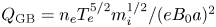 , depending on all eight uncertain inputs listed in table 1, obtained from our UQ and SA study in Farcaş et al. (Reference Farcaş, Merlo and Jenko2022), expressed using a Legendre basis, reads

It amounts to a multi-variate polynomial of third degree, comprising $47$ terms.
Appendix C. Out-of-bounds testing data
Table 2 shows the values of the Gene parameters $\{\omega _{T_e}, \eta _e, q, \tau, \beta _e, \lambda _{D}, \hat {s}, Z_{\mathrm {eff}}\}$ (columns two to nine) as well as the corresponding electron heat fluxes in GB units (last column) for the $40$
 out-of-bounds testing parameters used in § 4.2.2.
Table 2. Summary of the main parameters (columns two to nine, in the same units as in the main text) and of the corresponding GB-normalized electron heat flux (last column) for the 40 out-of-bounds testing parameters used to validate our proposed surrogate model.

Appendix D. Unit conversion
For simplicity, in the following we use superscript Fa22 to refer to quantities used in our original UQ study in Farcaş et al. (Reference Farcaş, Merlo and Jenko2022) and Fa24 to refer to quantities used in the present paper. Analogously, superscripts Ha22 and Ha24 are employed to refer to quantities specific to Hatch et al. (Reference Hatch, Michoski, Kuang, Chapman-Oplopoiou, Curie, Halfmoon, Hassan, Kotschenreuther, Mahajan, Merlo, Pueschel, Walker and Stephens2022) and Hatch et al. (Reference Hatch, Kotschenreuther, Li, Chapman-Oplopoiou, Parisi, Mahajan and Groebner2024), respectively.
In Farcaş et al. (Reference Farcaş, Merlo and Jenko2022), our simulations adopted the generalized Miller geometry using $R = 1.68\ \mathrm {m}$ , with the temperature gradient defined as

The conversion factor between $\omega _{T_e}^{\mathrm {Fa22}}$ in (D1) and $\omega _{T_e}^{\mathrm {Fa24}}$
 used in this paper is $4.6576$
 , therefore $\omega _{T_e}^{\mathrm {Fa24}} = \omega _{T_e}^{\mathrm {Fa22}}/4.5676$
 .
.
To use the model in (4.2) in the present work, we must (i) convert the temperature gradient and Debye length in our units to be compatible with the units used in (4.2) and (ii) convert the ensuing flux predictions to account for the area definition. The Debye length conversion is straightforward and was explained in the main text. To convert $\omega _{T_e}^{\mathrm {Fa24}}$ to $\omega _{T_e}^{\mathrm {Ha24}}$
 , we can use the chain rule to obtain

Using the definition of the Miller geometry, we can evaluate $\mathrm {d} r/ \mathrm {d} \psi$ in (D2) for any set of input parameters. The same is not true for $\psi _N/R$
 , which requires the knowledge of a global equilibrium. The value of this factor for our nominal parameters is 1/0.31, however, since the results of (4.2) linearly scale with it, it is clear that a model comparison is inevitably skewed by the specific choice of this factor. Since the model in (4.2) is richer than (4.1), we nevertheless employ it in § 4 for a more comprehensive overview using a constant value 1/0.20, which is close to the one for our nominal inputs.
The predictions $Q^{\mathrm {Ha24}}_{e}/Q^{\mathrm {Ha24}}_{\mathrm {GB}}$ provided by (4.2) can be converted to $Q^{\mathrm {Fa24}}_{e}/Q^{\mathrm {Fa24}}_{\mathrm {GB}}$
 as
as

where $A^{\mathrm {Ha24}} = 51.07\ \mathrm {m}^2$ and ${V^{\prime }}^{\mathrm {Ha22}} = 37.28\ \mathrm {m}^2$
 . Moreover, $Q^{\mathrm {Ha24}}_{\mathrm {GB}} = Q^{\mathrm {Fa24}}_{\mathrm {GB}} = Q^{\mathrm {Ha22}}_{\mathrm {GB}}$
 .
.


 Open access