


1. Introduction
As hardware computing power continues to advance, deep learning technologies have gradually transitioned from theory to practical applications. In this context, Visual Simultaneous Localization and Mapping (VSLAM) technology has once again garnered unprecedented attention and research efforts. VSLAM, as a crucial localization technique, is actively applied across various devices and domains, including robotics, autonomous driving, assistive technology for the visually impaired, and augmented reality. However, the presence of dynamic information in these application scenarios cannot be ignored, posing a significant challenge. Despite the overall maturity of VSLAM frameworks and the emergence of several high-precision and robust visual localization systems in the past two decades [Reference Davison, Reid, Molton and Stasse1–Reference Qin, Li and Shen3], it appears that these outstanding systems have not fully addressed the challenges and impacts of dynamic environments on visual localization.
Dynamic SLAM technology holds crucial significance in fields such as robotics and autonomous vehicles. It helps these systems achieve precise localization and collision avoidance in dynamic environments, thus enabling safer navigation. In the domains of intelligent surveillance, virtual reality, and augmented reality, dynamic SLAM can be used to track human movements, object mobility, and user positions in virtual environments, providing a more natural human–computer interaction experience. In industrial automation and logistics, dynamic SLAM is employed for real-time tracking of moving materials or robots, ensuring the safety and efficiency of production processes. However, effectively handling or harnessing dynamic information to improve the accuracy, robustness, and real-time capabilities of visual localization is the primary challenge in implementing these applications. This is essential for achieving greater autonomy and intelligence.
In such environments, the use of localization systems such as refs. [Reference Davison, Reid, Molton and Stasse1–Reference Qin, Li and Shen3] may be compromised by the presence of irregularly moving dynamic objects. This is because conventional VSLAM or Visual Odometry systems are typically based on maximum a posteriori estimation, which answers the question, “Under what conditions am I most likely to have observed these landmarks?” In the dynamic environment, actual observations may introduce landmarks associated with the unpredictable motion of these objects, making it challenging for the system to differentiate between its own motion and that of objects in the environment. This, in turn, affects the accuracy of localization results and can even lead to significant deviations in the construction of the environmental map.
In this paper, to address the issue of poor localization performance in dynamic environments, we delve into the unsolved problems and their essence. We propose a dynamic region segmentation method based on point cloud relativity. The main idea can be divided into two parts: firstly, utilizing the K-Means algorithm to cluster depth images, dividing them into multiple sub-point clouds, and then calculating the sub-pose between each sub-point cloud and a reference frame. Simultaneously, we introduce the concept of sub-point cloud dynamic–static relativity. By combining the dynamic–static relativity of sub-point clouds and sub-pose information, we can effectively identify which sub-point clouds belong to the dynamic point cloud. This process does not rely on epipolar geometry constraints and does not require prior knowledge of the approximate camera pose. Secondly, considering that motion is a continuous state, when new keyframes are inserted, we further refine the dynamic areas in the keyframes using weighted historical observation data. This refinement process not only enhances the system’s accuracy and robustness but also ensures the quality of the map. The SLAM method we propose is called CPR-SLAM.
This paper makes the following main contributions:
-
1. Segmentation method based on point cloud relativity: The paper introduces a method based on point cloud relativity for the segmentation of dynamic and static regions. This method has the distinctive feature of independent segmentation, as it does not require consideration of camera motion and eliminates the reliance on perspective transformations, which is a common dependency in most existing algorithms.
-
2. Refinement of dynamic areas in keyframes: Through the use of weighted historical observation data, the paper refines dynamic areas in keyframes about to be inserted, significantly enhancing the system’s robustness and localization accuracy.
-
3. Integration with ORBSLAM2 Artal System: The segmentation method is integrated into the ORBSLAM2 system, and evaluations and comparisons are performed using the TUM RGB-D benchmark dataset. Experimental results demonstrate that this approach substantially improves the robustness and localization accuracy of the ORBSLAM2 system.
The structure of the rest of the paper is as follows: Section 2 discusses related work, Section 3 provides details of the proposed method, Section 4 elaborates on the experimental results, and Section 5 presents conclusions and outlines future research directions.
2. Related work
In VSLAM within dynamic environments, two types of motion are observed in image sequences captured due to irregular camera movements: one is motion caused by the camera’s own motion, and the other is motion induced by independently moving objects. Typically, these motions can be distinguished using geometric-based methods and deep learning-based methods.
Geometric-based approaches in dynamic SLAM typically employ multiview geometry theory such as homography matrices and fundamental matrices to roughly estimate the camera’s own pose and correct image distortions resulting from camera motion. These methods attempt to differentiate between dynamic and static portions by analyzing the positional information of feature points or correspondences in the image sequence. Motion caused by the camera’s own movement is usually compensated for through pose estimation, while the remaining motion is considered to be caused by independently moving objects. These methods have a certain level of maturity in traditional VSLAM but still face challenges when dealing with rapid motion or a high number of dynamic objects.
Deep learning methods are increasingly being applied in dynamic SLAM. Deep learning can be used to recognize prior dynamic objects, as it can learn from extensive data and identify targets. Using deep learning network such as Convolutional Neural Networks (CNNs), known dynamic objects can be precluded, with most of the scene considered as static. This aids in compensating for image distortions caused by camera motion more accurately using geometric methods. The advantage of deep learning methods lies in their adaptability to large-scale data, particularly when handling complex dynamic scenes. However, the limitation of this approach is that it does not determine whether known objects are in motion; it treats them all as dynamic objects. Note that the key to dynamic SLAM is the identification of dynamic regions, not target recognition.
In summary, existing dynamic SLAM methods mostly rely on fake-static feature points, which are feature points that are difficult to determine as truly stationary, to compensate for image distortions caused by the camera’s own motion. However, some algorithms treat camera motion compensation and dynamic region identification as two separate tasks. This approach does not depend on all the operations before camera compensation, making it more widely applicable in various scenarios. Therefore, existing methods can be categorized into two main classes: those based on camera motion compensation estimation and those based on non-camera motion compensation estimation.
2.1. Based on camera motion compensation estimation
In Zhang et al. [Reference Zhang, Zhang, Jin and Yi4], they used homography matrices to compensate for the image motion caused by the camera’s own movement between two frames. They employed a differential approach to obtain the outlines of moving objects in the images and used the grayscale intensities of these outlines as weights in a particle filter to track these moving objects. In Chen and his team’s work [Reference Cheng, Wang and Meng5], they utilized the homography matrix to create the illusion that the camera remained approximately stationary between two adjacent frames. They then applied sparse optical flow within a Bayesian framework to compute the probability values for each grid cell in the images, ultimately using these probability values to segment dynamic regions. While these methods achieved good pose estimation results in dynamic environments, their underlying assumption was that static regions occupied the majority of the image. To mitigate the impact of the static region assumption on real-world environments in SLAM, many researchers have explored more robust outlier elimination algorithms [Reference Bahraini, Bozorg and Rad6–Reference Wang, Yao, Ma and Jing8]. Sun et al. [Reference Sun, Liu and Meng9], in their work, replaced the traditional Random Sample Consensus (RANSAC) algorithm, a probabilistic iterative approach, with the Least Median of Squares (LMED) algorithm [Reference Rousseeuw10]. The LMED algorithm can achieve results comparable to RANSAC but is more robust, making it suitable for a broader range of real-world scenarios.
Over the past few decades, with the rapid advancement of deep learning technology, some methods that combine the advantages of deep learning have achieved satisfactory localization accuracy. For example, in Chao et al. [Reference Yu, Liu, Liu, Xie, Yang, Wei and Fei11], SegNet [Reference Badrinarayanan, Kendall and Cipolla12], a lightweight semantic segmentation network, was used to identify potential dynamic objects and remove feature points within their regions. This was combined with RANSAC to calculate the fundamental matrix, and epipolar geometry constraints were used to remove unstable feature points that were not recognized. In ref. [Reference Ji, Wang and Xie13], the authors used a similar approach to DS-SLAM but focused on real-time performance by only recognizing dynamic regions in keyframes. To prevent false negatives due to untrained objects in the images and camera rotations, the authors clustered the depth information and calculated the mean reprojection error for each cluster to identify dynamic regions. In ref. [Reference Liu and Miura14], the authors utilized the OpenPose network [Reference Cao, Simon, Wei and Sheikh15] for pedestrian detection and used epipolar geometry constraints to determine dynamic regions. This method relied on human pose estimation for detecting potential dynamic objects and performed well indoors, where dynamic objects are typically humans. In ref. [Reference Li, Wang, Xu and Chen16], the authors employed the Mask R-CNN network [Reference He, Gkioxari, Dollár and Girshick17] for detection and, within a Bayesian framework, combined epipolar geometry’s epipolar line distance to assign dynamic probability values to each feature point, achieving precise localization.
2.2. Based on non-camera motion compensation estimation
Since most current methods require consideration of camera compensation, any missed or failed detections prior to camera compensation can significantly reduce the system’s localization accuracy and robustness. Many researchers have also started to focus on methods based on non-camera motion compensation estimation. For example, in Dai et al. [Reference Dai, Zhang, Li, Fang and Scherer18], they used a three-dimensional Delaunay triangulation method to establish correlations between points and embedded this method into the front end of ORBSLAM2 for dynamic object removal. This improvement enhanced localization accuracy compared to the original system. Similar to ref. [Reference Dai, Zhang, Li, Fang and Scherer18], Wang et al. [Reference Wang, Yao, Ma and Jing8] took a similar approach but, to enhance differentiation, used Delaunay triangulation only for keyframes to construct connections between points. They determined whether a point was dynamic by observing changes in distance between points in three-dimensional space. For ordinary frames, object tracking was implemented using template matching. While judging dynamic points based on relative positional information in three-dimensional space is an ingenious method in ideal conditions, it needs to account for issues such as depth errors caused by hardware limitations in RGB-D cameras. In Li et al. [Reference Li and Lee19], they introduced an intensity-assisted iterative closest point (ICP) approach. This method utilized edge point clouds in combination with intensity values to assist in the nearest neighbor iteration process. It was employed to determine point cloud distance weights between ordinary frames and keyframes, serving as an indicator for detecting dynamic targets. In ref. [Reference Kenye and Kala20], the authors used DNN-base object detection to obtain dynamic objects and then used foreground–background segmentation to preserve the background within the bounding boxes. Besides, multi-sensor fusion is also one of the solutions to the problem. He et al. [Reference He, Zhai, Feng, Zhang and Fu21] integrated two sensors, an Inertial Measurement Unit (IMU) and a stereo camera, using the IMU velocity as the camera’s own motion velocity. Simultaneously, they estimated the velocity of image feature points. They designed two filtering algorithms capable of effectively detecting dynamic feature points when moving objects dominate the scene in real environments captured within the images.
The above-mentioned methods are built upon traditional VSLAM systems and successfully break the strong assumption of a “static environment” in traditional VSLAM. However, they still have some limitations. Methods based on deep learning have limited categories for object recognition, high hardware requirements, and poor real-time performance and require predefined prior knowledge of target objects. Moreover, whether based on deep learning or geometric methods, most algorithms require accurate camera compensation before recognizing motion regions to achieve good localization accuracy. Some methods also struggle with non-rigidly moving objects. Under these layers of assumptions, the system’s applicability and robustness are significantly restricted, and its accuracy is reduced.
3. Proposed method
3.1. Problem statement
In this subsection, we provide a brief introduction to the difference between traditional VSLAM and VSLAM in dynamic environments. The VSLAM problem aims to estimate the camera’s own poses and landmarks by minimizing reprojection errors:
 \begin{equation} T*,x* = \mathop{\arg \min }\limits _{T,x}{\mkern 1mu} \sum \limits _{i = 1}^m{\sum \limits _{j = 1}^n{{w_{ij}}({{\left \|{{z_{ij}} +{V_{ij}} - h({T_{i,i - 1}},{x_j})} \right \|}^2})} } \end{equation}
In q. (1),
 $T^*$
and
$T^*$
and
 $x^*$
, respectively, represent the optimal pose and the landmark point.
$x^*$
, respectively, represent the optimal pose and the landmark point.
 $w({*})$
represents a robust kernel function.
$w({*})$
represents a robust kernel function.
 $h({*})$
denotes the process of projecting landmark points
$h({*})$
denotes the process of projecting landmark points
 $x_{j}$
from the previous frame
$x_{j}$
from the previous frame
 $i-1$
to the current frame
$i-1$
to the current frame
 $i$
through pose transformation
$i$
through pose transformation
 $T_{i,i-1}$
into the image coordinate system.
$T_{i,i-1}$
into the image coordinate system.
 $z_{ij}$
is the observation of the
$z_{ij}$
is the observation of the
 $j$
landmark point in the
$j$
landmark point in the
 $i$
frame, which represents the pixel values of the feature point indicated by
$i$
frame, which represents the pixel values of the feature point indicated by
 $x^{p}$
and
$x^{p}$
and
 $x^{q}$
in Fig. 1.
$x^{q}$
in Fig. 1.
 $V_{ij}$
denotes the velocity of motion from landmark point
$V_{ij}$
denotes the velocity of motion from landmark point
 $X^{q}$
to
$X^{q}$
to
 $X^{q'}$
, introduced by the irregular movement of the object, but it is not considered in traditional VSLAM. If
$X^{q'}$
, introduced by the irregular movement of the object, but it is not considered in traditional VSLAM. If
 $V_{ij}$
is not estimated or removed, the tartget function Eq. (1) will result in associating the feature point that should correspond to
$V_{ij}$
is not estimated or removed, the tartget function Eq. (1) will result in associating the feature point that should correspond to
 $x^{p}$
with
$x^{p}$
with
 $x^{q'}$
. Incorrect data association will lead to optimizing Eq. (1) in the wrong direction. Therefore, we need to eliminate the impact of
$x^{q'}$
. Incorrect data association will lead to optimizing Eq. (1) in the wrong direction. Therefore, we need to eliminate the impact of
 $V_{ij}$
on Eq. (1) before the pose estimation or integrate
$V_{ij}$
on Eq. (1) before the pose estimation or integrate
 $V_{ij}$
into Eq. (1) in a way that contributes positively.
$V_{ij}$
into Eq. (1) in a way that contributes positively.
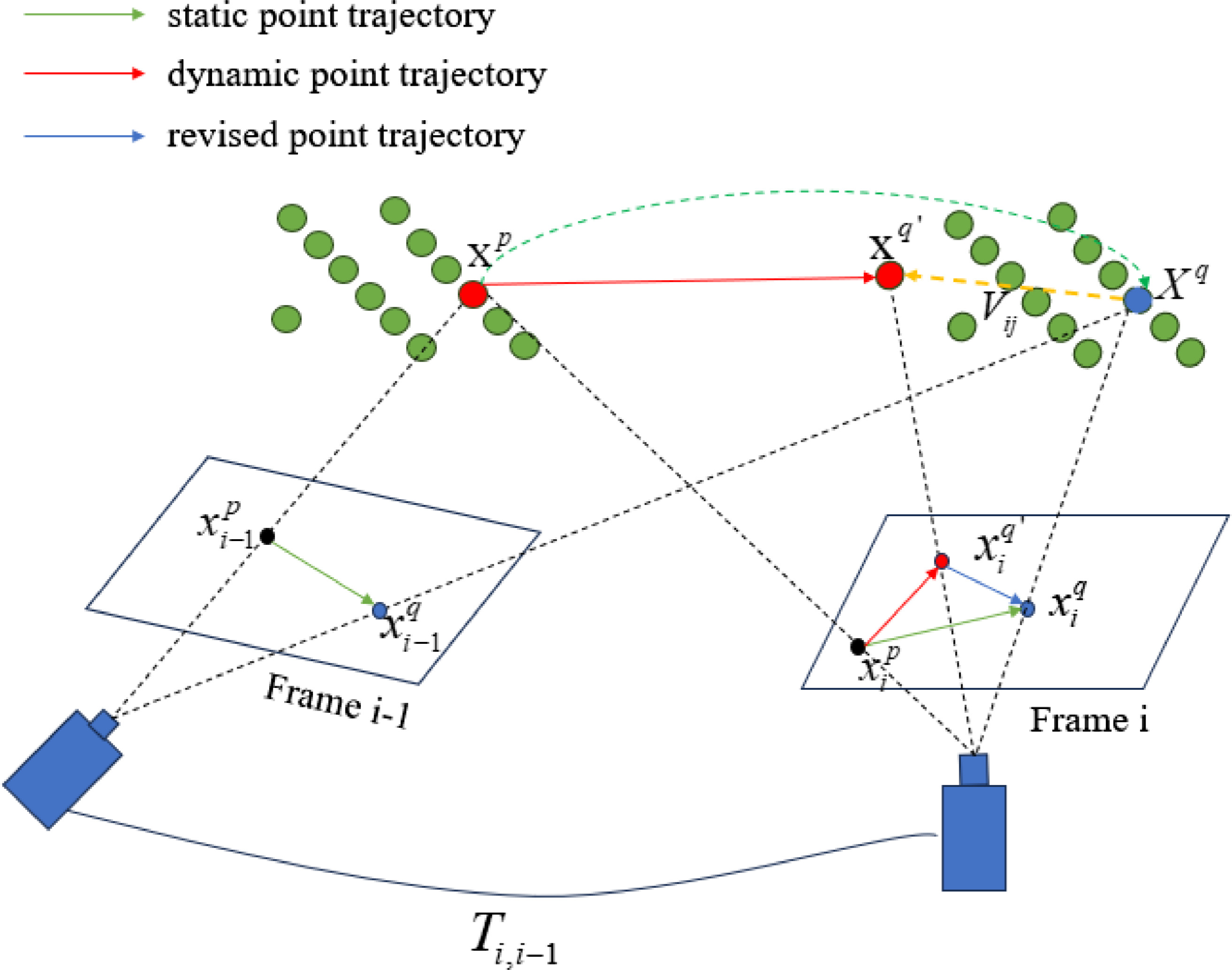
Figure 1. How dynamic feature points interfere with the analysis graph in traditional SLAM. Inside the quadrilateral are the two-dimensional points on the image, while outside are the three-dimensional points.
3.2. Method overview
Figure 2 illustrates an overview of our system. Our method serves as a front-end preprocessing step for the ORBSLAM2 system Artal, filtering out dynamic regions to reduce incorrect data associations. The system’s input requires RGB and depth images of the current frame for point cloud generation. Once processed, the current frame is temporarily stored in the system as a reference frame and will not be processed again.

Figure 2. The overview of CPR-SLAM. The gray box is the original ORBSLAM2 framework. Before the pose estimation, we add a dynamic region recognition module to remove dynamic feature points, as indicated by the blue box. For keyframes, we refine them using historical observation data, as shown in the yellow box.
The dynamic recognition module employs clustering algorithms to cluster the entire point cloud into multiple sub-point clouds. Then, it calculates the relative degree between these sub-point clouds in conjunction with the reference frame’s point cloud. Finally, it generates dynamic regions based on this relative degree. Feature points within these regions will not be used for camera pose estimation.
Additionally,in ORBSLAM2 Artal, keyframes represent the most representative frames in a sequence, helping to reduce redundancy in adjacent frames. They are crucial as they store map information, and subsequent optimizations are based on keyframes rather than ordinary frames. Thus, we have implemented a keyframe refinement module based on the tracking characteristics of ORBSLAM2. This module further refines the dynamic regions of keyframes using weight-based historical observation data. This approach mitigates the issue of reduced map point generation in keyframes due to false positives, ensuring the system’s robustness and accuracy.
3.3. Sub-point cloud construction
In dynamic environment, point cloud is mixed with noise generated by moving objects, so traditional ICP cannot be carried out directly. In order to enable the point cloud to recover part of the ability to calculate the pose transformation, we need to minimize the point cloud
 $P$
into a sub-point cloud
$P$
into a sub-point cloud
 $\{B_{1},B_{2},\ldots,B_{K}\}\in{P}$
.
$\{B_{1},B_{2},\ldots,B_{K}\}\in{P}$
.
Inspired by ref. [Reference Qian, Xiang, Wu and Sun22], to acquire geometric information from the environment and ensure real-time performance of the system, we adopted the data acquisition form of lidar to generate point clouds
 $P_{d}$
for the current frame. We sampled with intervals of
$P_{d}$
for the current frame. We sampled with intervals of
 $u=4$
rows and
$u=4$
rows and
 $v=4$
columns in pixels to accelerate the construction of KD tree, striking a balance between obtaining rich geometric information and maintaining real-time performance.
$v=4$
columns in pixels to accelerate the construction of KD tree, striking a balance between obtaining rich geometric information and maintaining real-time performance.
To avoid the defect that the point cloud only has geometric information, the point cloud intensity value is assigned during the voxel filtering of the point cloud. It not only improves ICP performance (Section 3.5), but also the accuracy of calculating the dynamic and static correlation of the sub-point cloud is ensured (Section 3.5). When assigning intensity values to the point cloud, we also perform further downsampling and remove a certain degree of noise points and outliers. We calculate the average grayscale value of all points within a cube of side length
 $l=0.05$
meter as the intensity value of the point cloud. Additionally, we use the centroid calculated from the points inside the cube to represent the geometric position of that region
$l=0.05$
meter as the intensity value of the point cloud. Additionally, we use the centroid calculated from the points inside the cube to represent the geometric position of that region
 $G_{i}$
, as in
$G_{i}$
, as in
 \begin{equation} \overline{I}_{G_{i}} = \sum _{x,y\in{G_{i}}}I(x,y) \end{equation}
 $\overline{I}_{G_{i}}$
is the intensity values of the i-th cube
$\overline{I}_{G_{i}}$
is the intensity values of the i-th cube
 $G_{i}$
, and
$G_{i}$
, and
 $I(x,y)$
denotes the gray value of pixel point coordinate (x, y).
$I(x,y)$
denotes the gray value of pixel point coordinate (x, y).
What is more, due to hardware limitations of RGB-D cameras, depth value errors follow a quadratic growth with distance [Reference Khoshelham and Elberink23]. Objects farther from the camera occupy a smaller portion of the field of view, resulting in fewer unstable feature points dominated by them, which has a smaller impact on camera motion estimation. To ensure the accuracy of dynamic object recognition, it is necessary to obtain precise point cloud position information. We need to eliminate unstable depth regions. Based on the noise model of depth cameras [Reference Nguyen, Izadi and Lovell24] and empirical values obtained through experiments, when the depth value exceeds 6 m, we set the depth value of the corresponding point in the depth image to 0.
Due to the original depth from RGB-D cameras, multiple layers or holes can appear in the point cloud structure. We use Moving Least Squares smoothing [Reference Lancaster and Salkauskas25] on the point cloud. Fig. 3 shows a side view of a point cloud of a planar wall. Due to camera hardware limitations and external factors, depth values become inaccurate, resulting in an irregular surface with irregularities in the point cloud. However, through point cloud smoothing, we can observe that the point cloud is closer to the true position information of the point cloud in the real environment. Additionally, point cloud smoothing significantly improves the accuracy of point cloud registration.
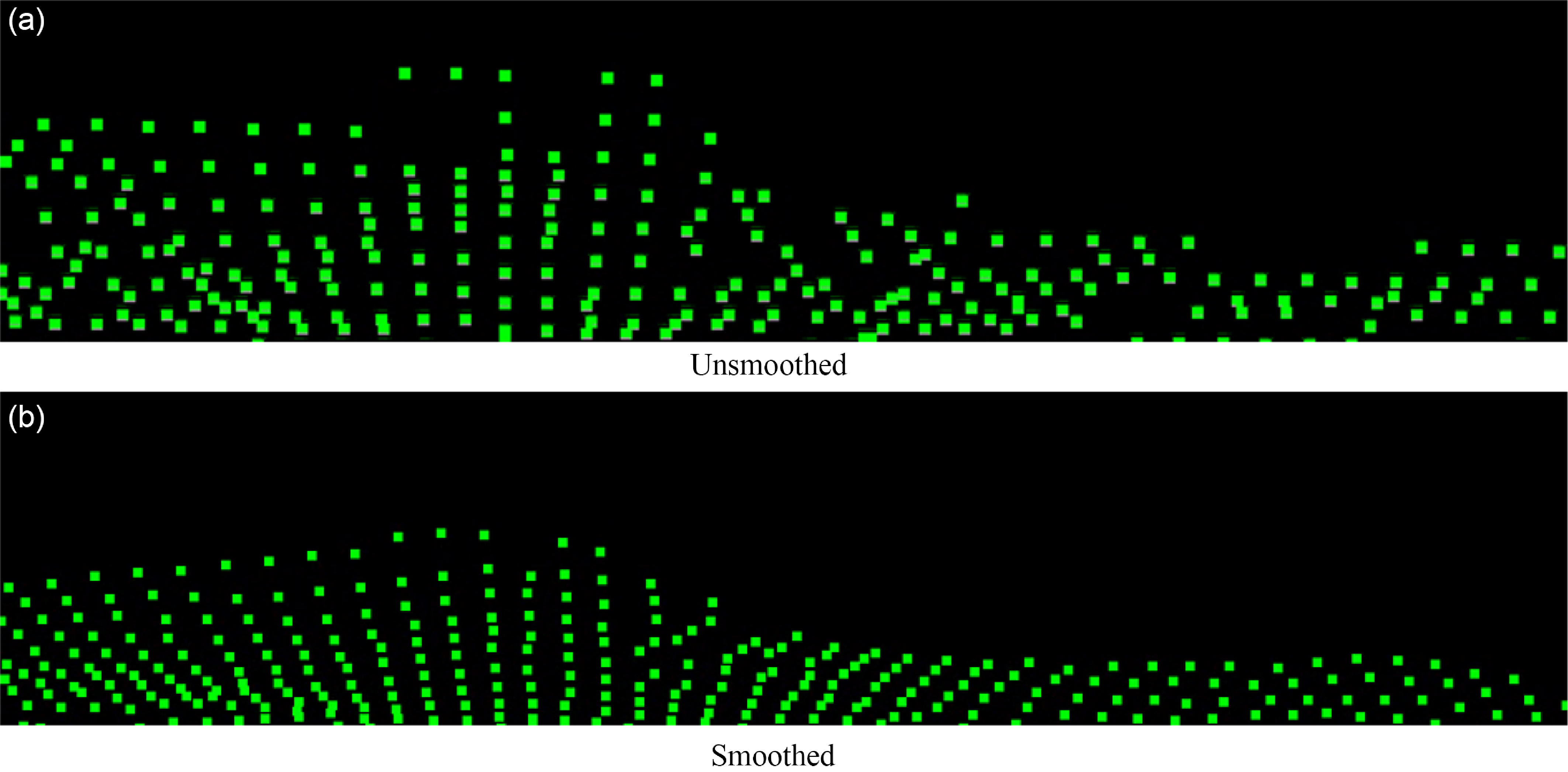
Figure 3. The three-dimensional visualization results of the smoothed point cloud and the unsmoothed point cloud are shown.
After this process, we obtain high-quality point cloud data, and then we use the K-Means clustering algorithm to cluster the point cloud into the empirical value
 $K=10$
sub-point clouds
$K=10$
sub-point clouds
 ${B}=\{B_{1},B_{2},\ldots,B_{K}\}$
.
${B}=\{B_{1},B_{2},\ldots,B_{K}\}$
.
3.4. Reference frame
In our experiment, we found that when the camera and the object move in approximately the same direction or speed, the algorithm is degraded. To minimize this affect, we take the previous
 $\sigma$
frames of the current frame as the reference frame. We cannot set
$\sigma$
frames of the current frame as the reference frame. We cannot set
 $\sigma$
to be too large; otherwise, the accuracy of static and dynamic correlation estimation will decline due to the large environmental difference. In our experiment, frame updates are faster than keyframes. Thus,
$\sigma$
to be too large; otherwise, the accuracy of static and dynamic correlation estimation will decline due to the large environmental difference. In our experiment, frame updates are faster than keyframes. Thus,
 $\sigma =5$
for the keyframes, while
$\sigma =5$
for the keyframes, while
 $\sigma =2$
for the frames.
$\sigma =2$
for the frames.
3.5. Estimation of sub-point cloud pose
In a dynamic environment, there are two types of sub-point clouds: dynamic sub-point clouds and static sub-point clouds, both of which change with the camera’s motion. In this scenario, all static sub-point clouds will undergo the same rigid transformation as the reference point cloud and exhibit motion opposite to the camera’s movement direction. Conversely, each dynamic sub-point cloud will have its unique motion and will not follow the same rigid transformation pattern.
In this subsection, we describe how to calculate the transformation matrix by registering each sub-point cloud
 $\{\lt P^j_{src}(i),I^j_{src}(i)\gt \}_{j\in (B),i\in{B_{j}}}$
of the source point cloud with the target point cloud
$\{\lt P^j_{src}(i),I^j_{src}(i)\gt \}_{j\in (B),i\in{B_{j}}}$
of the source point cloud with the target point cloud
 $P_{tgt}$
of the reference frame, the transformation called the sub-pose.
$P_{tgt}$
of the reference frame, the transformation called the sub-pose.
 $P^j_{src}(i)$
represents the i-th point in the j-th sub-point cloud in the sub-point cloud
$P^j_{src}(i)$
represents the i-th point in the j-th sub-point cloud in the sub-point cloud
 $B$
.
$B$
.
 $I^j_{src}(i)$
represents intensity value of the i-th point in the j-th sub-point cloud in the sub-point cloud
$I^j_{src}(i)$
represents intensity value of the i-th point in the j-th sub-point cloud in the sub-point cloud
 $B$
. In the process of processing, the sub-point cloud is a small part of the source point cloud. It will fall into the local optimal solution, resulting in the wrong identification of dynamic region, if traditional ICP is used. Inspired by the work in Li et al. [Reference Li and Lee26], we adopted a registration estimation method that combines grayscale information with ICP and traditional ICP. Grayscale ICP utilizes the point cloud’s grayscale values as intensity information for point correspondence, effectively avoiding the problem of getting stuck in local minima during local area matching. To reduce computational complexity, we use grayscale ICP for registration in the initial iterations. Once grayscale ICP iterations are completed, we then employ traditional ICP for further refinement to obtain more precise point cloud registration results. This strategy aims to ensure registration accuracy while effectively controlling computational costs. Grayscale ICP is an iterative approach that estimates the optimal pose matrix by minimizing the weighted Euclidean distance between the target point cloud and the source point cloud. The specific process is as follows.
$B$
. In the process of processing, the sub-point cloud is a small part of the source point cloud. It will fall into the local optimal solution, resulting in the wrong identification of dynamic region, if traditional ICP is used. Inspired by the work in Li et al. [Reference Li and Lee26], we adopted a registration estimation method that combines grayscale information with ICP and traditional ICP. Grayscale ICP utilizes the point cloud’s grayscale values as intensity information for point correspondence, effectively avoiding the problem of getting stuck in local minima during local area matching. To reduce computational complexity, we use grayscale ICP for registration in the initial iterations. Once grayscale ICP iterations are completed, we then employ traditional ICP for further refinement to obtain more precise point cloud registration results. This strategy aims to ensure registration accuracy while effectively controlling computational costs. Grayscale ICP is an iterative approach that estimates the optimal pose matrix by minimizing the weighted Euclidean distance between the target point cloud and the source point cloud. The specific process is as follows.
3.5.1. The initial pose
According to ORBSLAM2’s constant velocity model,
 \begin{equation} \widehat{T} = (T_{pre}T_{last})^{-1}T_{ref} \end{equation}
 $T_{pre}$
represents the increment of pose transformation between the last two adjacent frames in the world coordinate system,
$T_{pre}$
represents the increment of pose transformation between the last two adjacent frames in the world coordinate system,
 $T_{last}$
the camera pose of the last frame, and
$T_{last}$
the camera pose of the last frame, and
 $T_{ref}$
the pose of the reference frame. The initial pose can effectively prevent falling into the local optimal solution and accelerate the iteration speed.
$T_{ref}$
the pose of the reference frame. The initial pose can effectively prevent falling into the local optimal solution and accelerate the iteration speed.
3.5.2. Search the corresponding points
Search the corresponding points between the sub-point cloud
 $P^j_{src}(i)$
and the target point cloud according to the initial pose. The nearest neighbor search seeks
$P^j_{src}(i)$
and the target point cloud according to the initial pose. The nearest neighbor search seeks
 $\alpha =10$
nearest point as candidate point
$\alpha =10$
nearest point as candidate point
 $\{c_{i}\}^\alpha _{i=0}$
, calculates their matching degree and finally selects the highest degree
$\{c_{i}\}^\alpha _{i=0}$
, calculates their matching degree and finally selects the highest degree
 $S(i,k)$
as corresponding point
$S(i,k)$
as corresponding point
 $\widetilde{P_{tgt}}(c_{*})$
.
$\widetilde{P_{tgt}}(c_{*})$
.
 \begin{equation} S(i,k) ={\underset{k\in{c_{1},c_{2},\ldots,c_{\alpha }}}{\arg \max }w(r^G(k))w(r^I(k))} \end{equation}
 \begin{equation} r^G(k) = \|\Delta TP^j_{src}(i)-P_{tgt}(k)\| \end{equation}
 \begin{equation} r^I(k) = \|I^j_{src}(i)-I_{tgt}(k)\| \end{equation}
 $\Delta T$
is the incremental matrix for each iteration.
$\Delta T$
is the incremental matrix for each iteration.
 $r^G(*)$
is geometric residuals.
$r^G(*)$
is geometric residuals.
 $r^I(*)$
is intensity residuals.
$r^I(*)$
is intensity residuals.
 $w(*)$
is weight conversion function.
$w(*)$
is weight conversion function.
Following the weighting conversion function based on t-distribution of a student [Reference Kerl, Sturm and Cremers27], and we also assume that the two residuals obey t-distribution. Therefore, The weight conversion function can be expressed as
 \begin{equation} w = \frac{v-1}{v+\frac{r^{(*)}-\mu ^{(*)}}{\sigma ^{(*)}}} \end{equation}
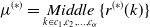 \begin{equation} \mu ^{(*)} ={\underset{k\in{c_{1},c_{2},\ldots,c_{\alpha }}}{Middle}\{r^{(*)}(k)\}} \end{equation}
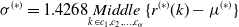 \begin{equation} \sigma ^{(*)} = 1.4268{\underset{k\in{c_{1},c_{2},\ldots,c_{\alpha }}}{Middle}\{r^{(*)}(k)-\mu ^{(*)}\}} \end{equation}
 $v$
is the degree of freedom of the t-distribution, and we set it to 5.
$v$
is the degree of freedom of the t-distribution, and we set it to 5.
 $\mu ^{(*)}$
represents the median of geometric or intensity residuals; also
$\mu ^{(*)}$
represents the median of geometric or intensity residuals; also
 $\sigma ^{(*)}$
is variance.
$\sigma ^{(*)}$
is variance.
3.5.3. Calculate the gain
 $\Delta T$

Calculate the gain
 $\Delta T$
to minimize the sum of the global Euclidean distances, as in
$\Delta T$
to minimize the sum of the global Euclidean distances, as in
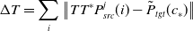 \begin{equation} \Delta T = \sum \limits _i{\left \|{T{T^*}P_{src}^j(i) -{{\tilde P}_{tgt}}({c_*})} \right \|} \end{equation}
3.5.4. Update
Add the computed increments to the optimal pose transformation matrix. Update
 $T^*$
as
$T^*$
as
 \begin{equation} {T^*} \leftarrow \Delta T{T^*} \end{equation}
All sub-point clouds can be registered according to the above method to obtain
 $\{{T_{{B_i}}}\} _{i = 0}^K$
. This method can reduce the possibility of falling into local solution effectively and can improve the accuracy of each point correctly matching corresponding points.
$\{{T_{{B_i}}}\} _{i = 0}^K$
. This method can reduce the possibility of falling into local solution effectively and can improve the accuracy of each point correctly matching corresponding points.
3.6. Correlation degree estimation
We will get the transformation matrix
 $\{{T_{{B_i}}}\} _{i = 0}^K$
to transform the source point cloud and estimate the degree of correlation between each block sub-point cloud. Find the nearest point
$\{{T_{{B_i}}}\} _{i = 0}^K$
to transform the source point cloud and estimate the degree of correlation between each block sub-point cloud. Find the nearest point
 ${P_{tgt}}(j)$
of the i-th point
${P_{tgt}}(j)$
of the i-th point
 $\hat P_{src}^j(i)$
and calculate its euclidean distance. In order to prevent a point from being matched to multiple points, show as Fig. 4, an additional intensity value is used as a penalty to find the corresponding point. Cumulative scores of all points are averaged as the score of the correlation degree:
$\hat P_{src}^j(i)$
and calculate its euclidean distance. In order to prevent a point from being matched to multiple points, show as Fig. 4, an additional intensity value is used as a penalty to find the corresponding point. Cumulative scores of all points are averaged as the score of the correlation degree:
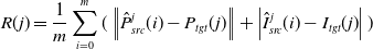 \begin{equation} R(j) = \frac{1}{m}\sum \limits _{i = 0}^m{(\left \|{\hat P_{src}^j(i) -{P_{tgt}}(j)} \right \|} + \left |{\hat I_{src}^j(i) -{I_{tgt}}(j)} \right |) \end{equation}
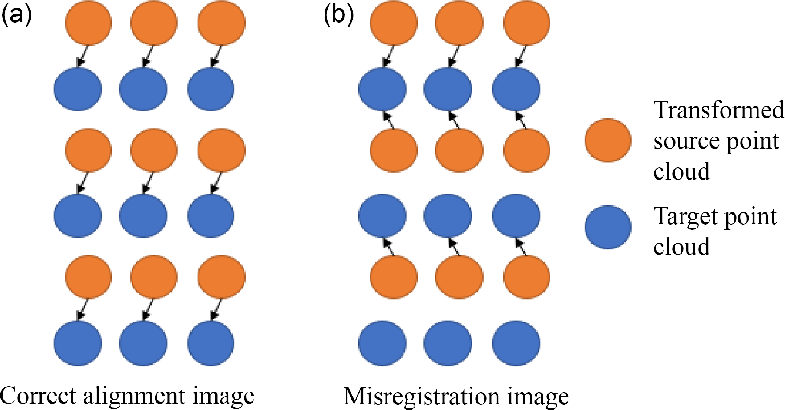
Figure 4. In figure (a), a correct point cloud matching schematic is shown, where each point has a unique corresponding point. In figure (b), there is a case where one point corresponds to multiple points, which often occurs in edge point clouds.
 $m$
is the total number of the sub-point cloud.
$m$
is the total number of the sub-point cloud.
 $\hat P_{src}^j(i)$
is the i-th point in a transformed point cloud. It is obtained by the source point cloud through the pose transformation matrix
$\hat P_{src}^j(i)$
is the i-th point in a transformed point cloud. It is obtained by the source point cloud through the pose transformation matrix
 $T_{{B_j}}$
of the j-th sub-point cloud, as follows:
$T_{{B_j}}$
of the j-th sub-point cloud, as follows:
 \begin{equation} \hat P_{src}^j \leftarrow{P_{src}}{T_{Bj}} \end{equation}
3.7. Reject dynamic region
If there are sub-point clouds with the same motion (e.g., static sub-point clouds with only camera motion), it can be estimated from the transformation matrix that the source and target point clouds are approximately coincident. Therefore, based on the poses of the sub-point clouds in space, dynamic and static sub-point clouds can be effectively distinguished. To sum up, we divide all sub-point clouds into two groups: the dynamic correlation group and the static correlation group.
Since the score
 $\{ R(j)\} _{j \in K}$
varies, we find it difficult to use a fixed threshold to determine the state of the sub-point cloud. To some extent, this is similar to a binary classification problem in machine learning. Using the mean absolute error [Reference Error28] as a dynamic threshold to distinguish between dynamic and static sub-point clouds yielded remarkable results. The threshold value is as follows:
$\{ R(j)\} _{j \in K}$
varies, we find it difficult to use a fixed threshold to determine the state of the sub-point cloud. To some extent, this is similar to a binary classification problem in machine learning. Using the mean absolute error [Reference Error28] as a dynamic threshold to distinguish between dynamic and static sub-point clouds yielded remarkable results. The threshold value is as follows:
 \begin{equation} \varepsilon = \mu + 1.4826Mid\{ R(j) - \partial \} _{j = 0}^K \end{equation}
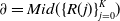 \begin{equation} \partial = Mid(\{ R(j)\} _{j = 0}^K) \end{equation}
 \begin{equation} \mu = \frac{1}{K}\sum \limits _{i = 1}^k{R(i)} \end{equation}
 $K$
is the number of cluster. The threshold can effectively distinguish which point clouds belong to static point clouds:
$K$
is the number of cluster. The threshold can effectively distinguish which point clouds belong to static point clouds:
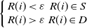 \begin{equation} \left \{{\begin{array}{*{20}{c}}{R(i) \lt \varepsilon }&{R(i) \in S}\\{R(i) \gt \varepsilon }&{R(i) \in D} \end{array}} \right . \end{equation}
 $S$
represents static sub-point group, while
$S$
represents static sub-point group, while
 $D$
belongs to dynamic sub-point group. All point clouds belonging to
$D$
belongs to dynamic sub-point group. All point clouds belonging to
 $D$
group will be projected onto the camera plane to generate mask. Since point clouds only occupy one-pixel space on the camera plane, we need to draw a circle centered on the projection point and fill it. In the end, we obtain dynamic masks through morphologic geometry. The feature points in the mask will not be included in the pose estimation of the camera.
$D$
group will be projected onto the camera plane to generate mask. Since point clouds only occupy one-pixel space on the camera plane, we need to draw a circle centered on the projection point and fill it. In the end, we obtain dynamic masks through morphologic geometry. The feature points in the mask will not be included in the pose estimation of the camera.
3.8. Keyframe refinement
Due to the influence of degraded environment, the sub-point cloud is false negative (static recognition becomes dynamic). Besides, from the experiments, we found that this method can partially mitigate the drawbacks of a fixed number of clusters. We combine the characteristics of ORBSLAM2 that the map points generated by the keyframes will determine the tracking performance of the subsequent ordinary frames. We will use multiple observations from regular frames; it is the dynamic region mask generated by the dynamic recognition module from regular frames, to refine the dynamic regions generated by keyframes. In fact, when there is new keyframe insertion, we take the previous
 $N$
frame masks as historical observation data rather than all of them. Estimate the weight of pixel points as follows:
$N$
frame masks as historical observation data rather than all of them. Estimate the weight of pixel points as follows:
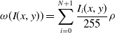 \begin{equation} \omega (I(x,y)) = \sum \limits _{i = 0}^{N + 1}{\frac{{I_i}(x,y)}{255}\rho } \end{equation}
 ${I_i}(x,y)$
is the pixel with coordinates (x,y) of the i-th data observation.
${I_i}(x,y)$
is the pixel with coordinates (x,y) of the i-th data observation.
 $\rho$
is the weight of pixel. Since keyframes are refined, their credibility is higher than that of frames, so the
$\rho$
is the weight of pixel. Since keyframes are refined, their credibility is higher than that of frames, so the
 $\rho$
for keyframes is 3. In contrast, for ordinary frames,
$\rho$
for keyframes is 3. In contrast, for ordinary frames,
 $\rho =2$
. In our experiment, N is set to 6. The plus one denotes the current keyframe; we want to ensure that all dynamic objects can be recognized. We do not consider the keyframes generated between the first N frames, because the environmental change between the keyframe and the reference frame is relatively large, which is easy to misdetect. When the pixel weight is
$\rho =2$
. In our experiment, N is set to 6. The plus one denotes the current keyframe; we want to ensure that all dynamic objects can be recognized. We do not consider the keyframes generated between the first N frames, because the environmental change between the keyframe and the reference frame is relatively large, which is easy to misdetect. When the pixel weight is
 $\tau$
times greater than the weight of total observation, we regard it as a dynamic pixel:
$\tau$
times greater than the weight of total observation, we regard it as a dynamic pixel:
 \begin{equation} \left \{{\begin{array}{*{20}{c}}{\omega (I(x,y)) \lt \tau (N+1)\rho }&{I(x,y) = 0}\\{\omega (I(x,y)) \gt \tau (N+1)\rho }&{I(x,y) = 1} \end{array}} \right . \end{equation}
It is worth noting that
 $\tau =0.6$
exhibited the best performance in our experiments. This value indicates the proportion of historical observation dataset where motion was detected in certain areas. In the experiment, it was found that the feature points are easy to generate on the edge of the object, and those are unstable. Hence, the mask generated by the refined keyframe will be properly expanded so that the edge points will not participate in the pose estimation process of the camera. It is summarized in Algorithm 1.
$\tau =0.6$
exhibited the best performance in our experiments. This value indicates the proportion of historical observation dataset where motion was detected in certain areas. In the experiment, it was found that the feature points are easy to generate on the edge of the object, and those are unstable. Hence, the mask generated by the refined keyframe will be properly expanded so that the edge points will not participate in the pose estimation process of the camera. It is summarized in Algorithm 1.
Algorithm 1 Keyframe refinement algorithm

4. Experiment
4.1. Overview
Validate the validity of our approach on the TUM dataset, which is widely used to evaluate VSLAM. We integrated the dynamic area identification approach into ORBSLAM2 and used ORBSLAM2 as a baseline to demonstrate our improvements. Initially, we assessed the outcomes of various modules presented in this paper. Subsequently, we compared our results with exceptional dynamic VSLAM approaches, encompassing geometric and deep learning methods. Finally, we demonstrated the effectiveness and performance of our method using an RGB-D camera in real-world scenarios.
4.2. Dataset
In the TUM dataset, we selected four highly dynamic sequences fr3/walking (termed as fr3/w) and two low dynamic sequences fr3/sitting (termed as fr3/s), denoted with a “*”. Each sequence contains RGB images and corresponding depth images with size 640×480. Ground truth poses are provided by a high-precision pose capture system. Within the TUM dataset, fr3/w involves two individuals moving around a table along with other object movements. fr3/s depicts two individuals sitting on chairs with slight limb movements. The camera operates in four distinct motion states indicated by suffixes: static (indicating slight camera motion that approximates stillness), translation along three axes (xyz), rotation along principal axes (rpy), and movement along a hemisphere with a 1 m diameter (half). These sequences pose significant challenges, often experiencing environmental degradation, such as instances where the camera moves in the same direction as people. In some sequences, over half of the camera’s field of view is occupied by moving objects. Parameters required for the experiments are specified in Section 3.
4.3. Evaluation metrics
The evaluation metrics commonly used for assessing camera pose estimation errors are the Root Mean Square Error (RMSE) and Standard Deviation (SD) of the Absolute Trajectory Error (ATE), which indicate the global trajectory consistency. Additionally, Relative Pose Error (RPE) consists of relative rotation (m/s) and relative translation (
 $^{\circ }$
/s), indicating the drift per second in odometry. To mitigate algorithmic variability and obtain quantitative results with practical reference value, multiple sets of experiments were conducted on all experimental data, and the median value was used as the final result. Except for the method proposed in this paper, other evaluation data are from the corresponding papers, “–” meaning that the original data is not public.
$^{\circ }$
/s), indicating the drift per second in odometry. To mitigate algorithmic variability and obtain quantitative results with practical reference value, multiple sets of experiments were conducted on all experimental data, and the median value was used as the final result. Except for the method proposed in this paper, other evaluation data are from the corresponding papers, “–” meaning that the original data is not public.
4.4. Experimental equipment
As shown in Fig. 5, all experiments are conducted on an Nvidia Jetson AGX Orin embedded platform with a 12-core v8.2 64-bit CPU and 32 GB of memory, running Ubuntu 20.04 and Robot Operating System (ROS). It is important to note that GPU acceleration was not used for data processing in the experiments. In real-world scenarios, a Realsense D455i camera was used as the RGB-D sensor to capture image and depth information. In addition, OptriTrack, show in Fig. 6, is a motion capture system consisting of nine cameras. The average error of OptriTrack calibration is 0.646 mm. We used mark points to create a camera rigid body and then obtained the actual camera trajectory. The power bank is used to supply power to the Jetson AGX Orin. In the experiment, a laptop is used as a monitor.

Figure. 5. A wheeled robot.
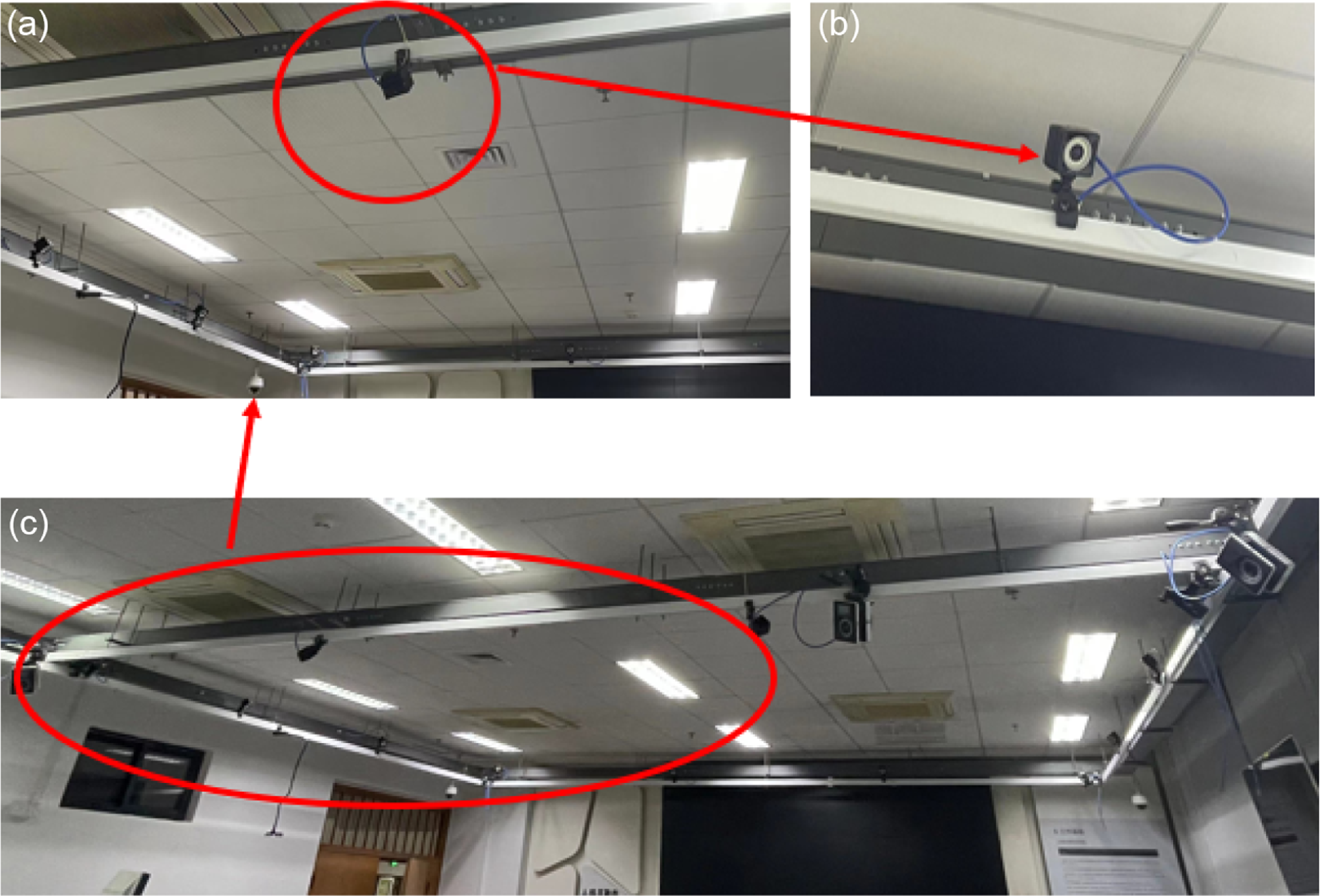
Figure. 6. The OptriTrack equipment.
4.1.1. Performance of dynamic area identification
Dynamic region recognition plays a crucial role in the accuracy of front-end data association of VSLAM. The qualitative results are shown in Fig. 7. Each sequence provides two illustrative images for visual analysis. As shown in Fig. 7, the proposed method has high accuracy in dynamic region detection. In Fig. 7 (a), it can be accurately identified even if only a small head is moving. In addition, the deep learning-based method is very sensitive to camera rotation, which often leads to missing detection. Figure 7 (c, h, i) fully shows that our detection method has certain anti-interference ability to camera rotation. Figure 7 (j) shows a person dressed in black is pulling a chair, and the chair is transformed from static to dynamic, which cannot be recognized by the untrained network. Surprisingly, the method proposed in this paper can quickly recognize the chair as a dynamic area, avoiding missing detection of dynamic objects.

Figure 7. Qualitative results of dynamic target detection. For each sequence, two results are provided as visualization. The same column is the recognition result of the same sequence. The first row and the third row are the tracking feature point results. The second row and the fourth row are the dynamic region mask.
4.1.2. Performance of keyframe refinement
We will verify whether keyframe refinement can improve the local accuracy of the system. As Table I shows, the overall effect of Fr3/s/xyz and Fr3/s/half for low dynamic sequences is not significantly improved, but for both high dynamic sequences, it is. One reason is that the clustering algorithm will cluster them together when moving objects and some static objects are close to each other. The other one is environment overfits, it is a common problem with most geometric-based methods. The historical observation data can remedy the appearance. It makes the keyframe generate more stable static landmarks, which is well shown in Fig. 8.
Table I. Comparison of RMSE of the Absolute Trajectory Error (ATE). The (O) is the original keyframe processing, and the (R) is refined keyframe. The best results are highlighted in bold (m).

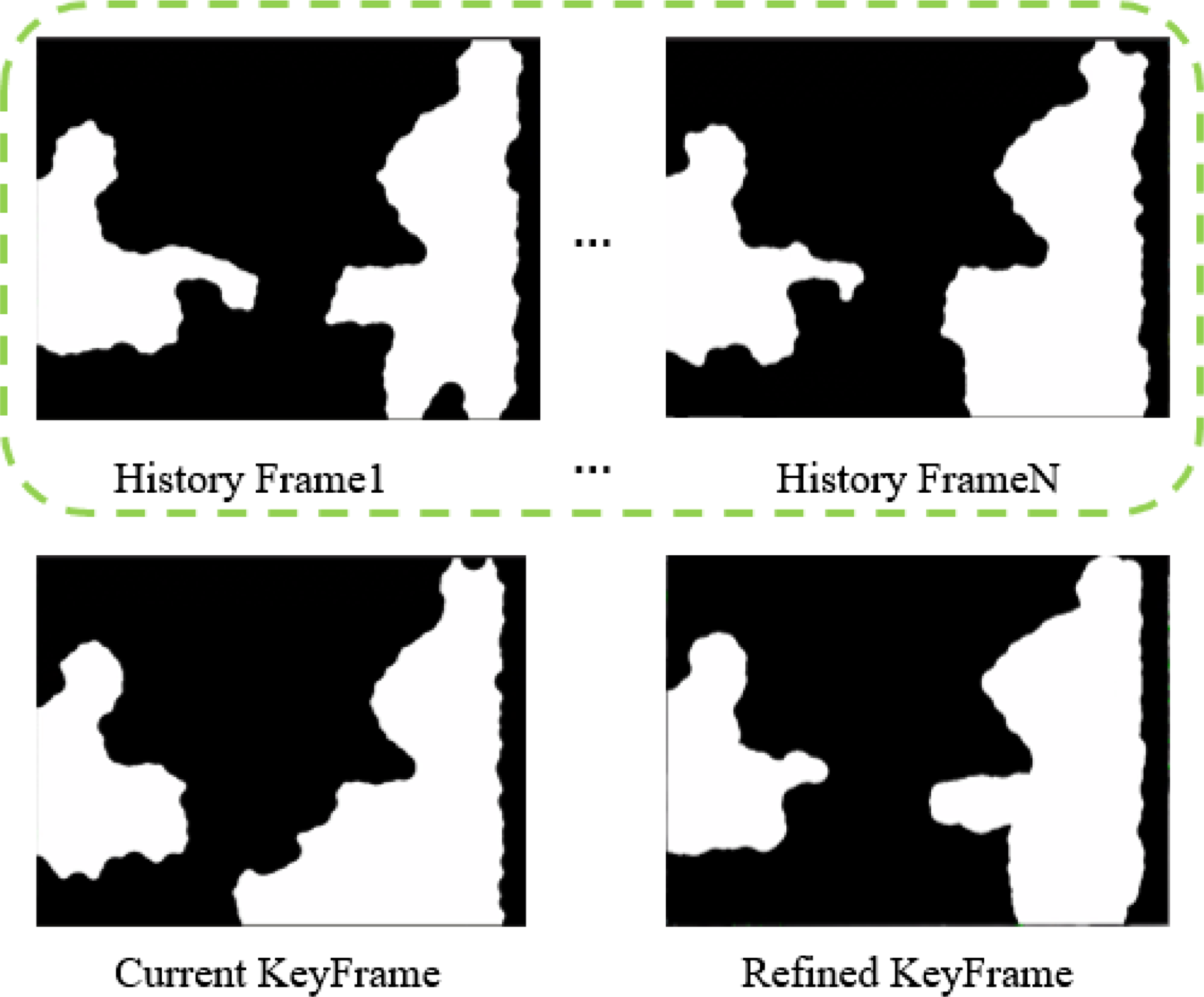
Figure 8. The green box is the historical observation result of multiple frames.
4.1.3. Performance of visual localization
In order to reflect that our method improves the local performance of ORBSLAM2 in dynamic environment, we present the RMSE and SD of ATE in Table II, which are more able to illustrate the robustness and stability of the system.
Table II. Comparison of RMSE of the Absolute Trajectory Error (ATE). The best results are highlighted in bold (m).

In Table II, CPR-SLAM can improve the performance of most highly dynamic sequences by an order of magnitude, up to 98.36% for RMSE and 98.43% for SD. The results show that the method significantly improves the local accuracy and system robustness of ORBSLAM2 in dynamic. Unfortunately, CPR-SLAM has shown a slight decrease in performance in the low dynamic sequence Fr3/s/xyz, with a 22.91% increase in RMSE compared to ORBSLAM2. This decrease was attributed to occasional false negatives in the method, resulting in a reduction in the number of feature points and an uneven distribution. In practice, ORBSLAM2 is still unable to effectively eliminate dynamic points in most cases; therefore, we can obtain more accurate camera’s pose estimation after identifying dynamic areas. In order to provide a more intuitive sense of the algorithm’s performance, we utilize the ground truth provided by TUM and a trajectory plotting program to generate trajectory plots, as shown in Fig. 9. The algorithm presented in this paper not only avoids significant frame loss but also closely follows the real trajectory.
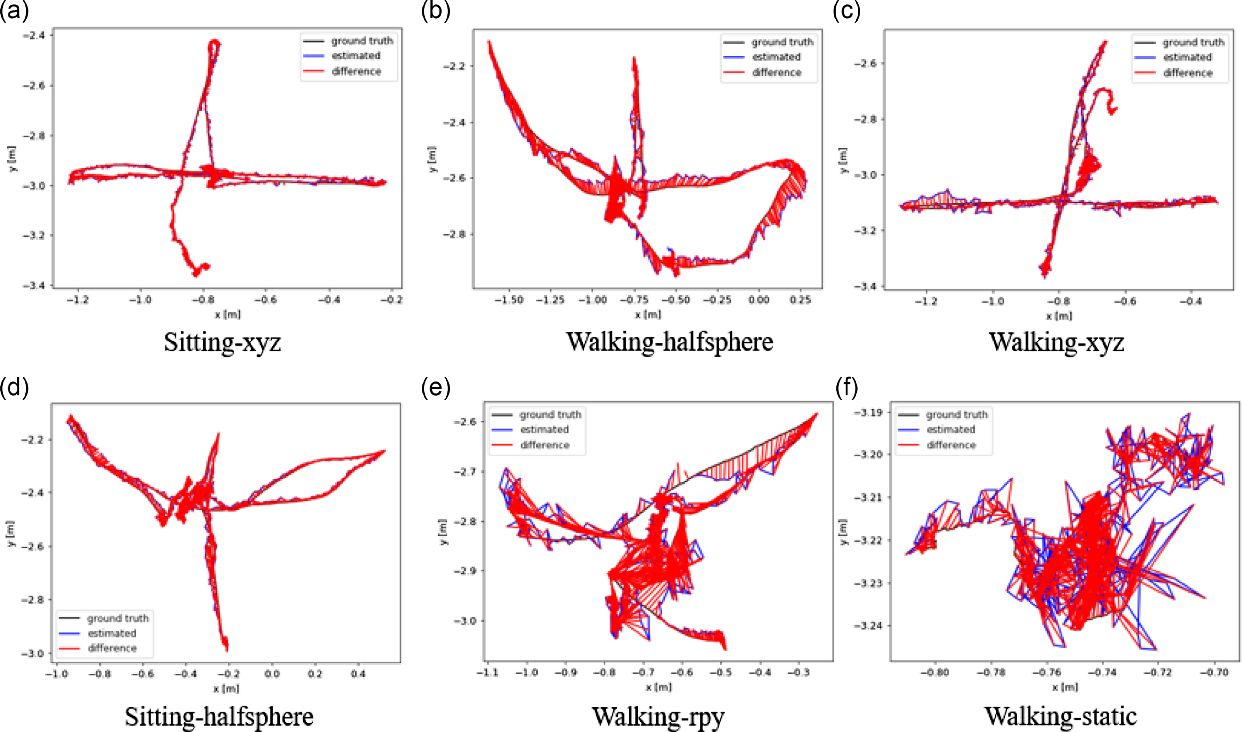
Figure 9. Comparison with the actual trajectory. The red line indicates the difference between the estimated trajectory and the ground truth. A shorter red line indicates higher localization accuracy.
4.1.4. Comparison with state of the arts
We compare our results with state-of-the-art dynamic VSLAM, based on the geometric approach: PC [Reference Dai, Zhang, Li, Fang and Scherer18], SPW [Reference Li and Lee19], and StaticFusion [Reference Scona, Jaimez, Petillot, Fallon and Cremers29]. Based on deep learning, methods like KMOP-VSLAM [Reference Liu and Miura14], Detect-SLAM [Reference Zhong, Wang, Zhang and Wang30], and EM-fusion [Reference Strecke and Stuckler31] are popular in the industry. These excellent methods adopt different dynamic detection algorithms, making them of certain comparative value. The results of ATE are presented in Table III, while the results of RPE are summarized in Tables IV and V.
Table III. Comparison of RMSE of the Absolute Trajectory Error (ATE). The best results are highlighted in bold. * indicates learning-based methods. We use the results published in their original papers when applicable (m).
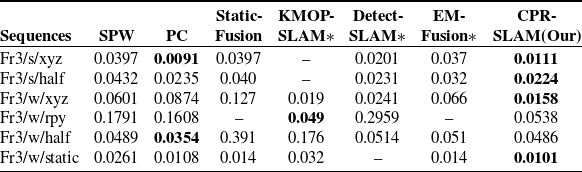
Table IV. Comparison of RMSE of the Relative Pose Error (RPE) in translational drift. The best results are highlighted in bold (m/s).
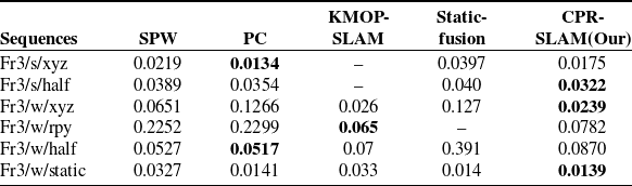
Table V. Comparison of RMSE of the Relative Pose Error (RPE) in rotational drift. The best results are highlighted in bold (
 $^{\circ }$
/s).
$^{\circ }$
/s).

Table III shows that the algorithm proposed in this paper achieves leading results in multiple test sequences. Although it lags behind in Fr3/w/rpy and Fr3/w/half under high dynamics, the overall localization accuracy results are still quite competitive. From Tables IVand V, it can be observed that the algorithm proposed in this paper demonstrates satisfactory results, indicating that the algorithm presented in this paper exhibits high stability. In particular, the SPW method also uses point cloud to detect the moving region, and CPR-SLAM has better performance among the indexes in the Tables III–V. The comparison results are consistent with Fig. 10. It can be seen that our algorithm has fewer red lines.
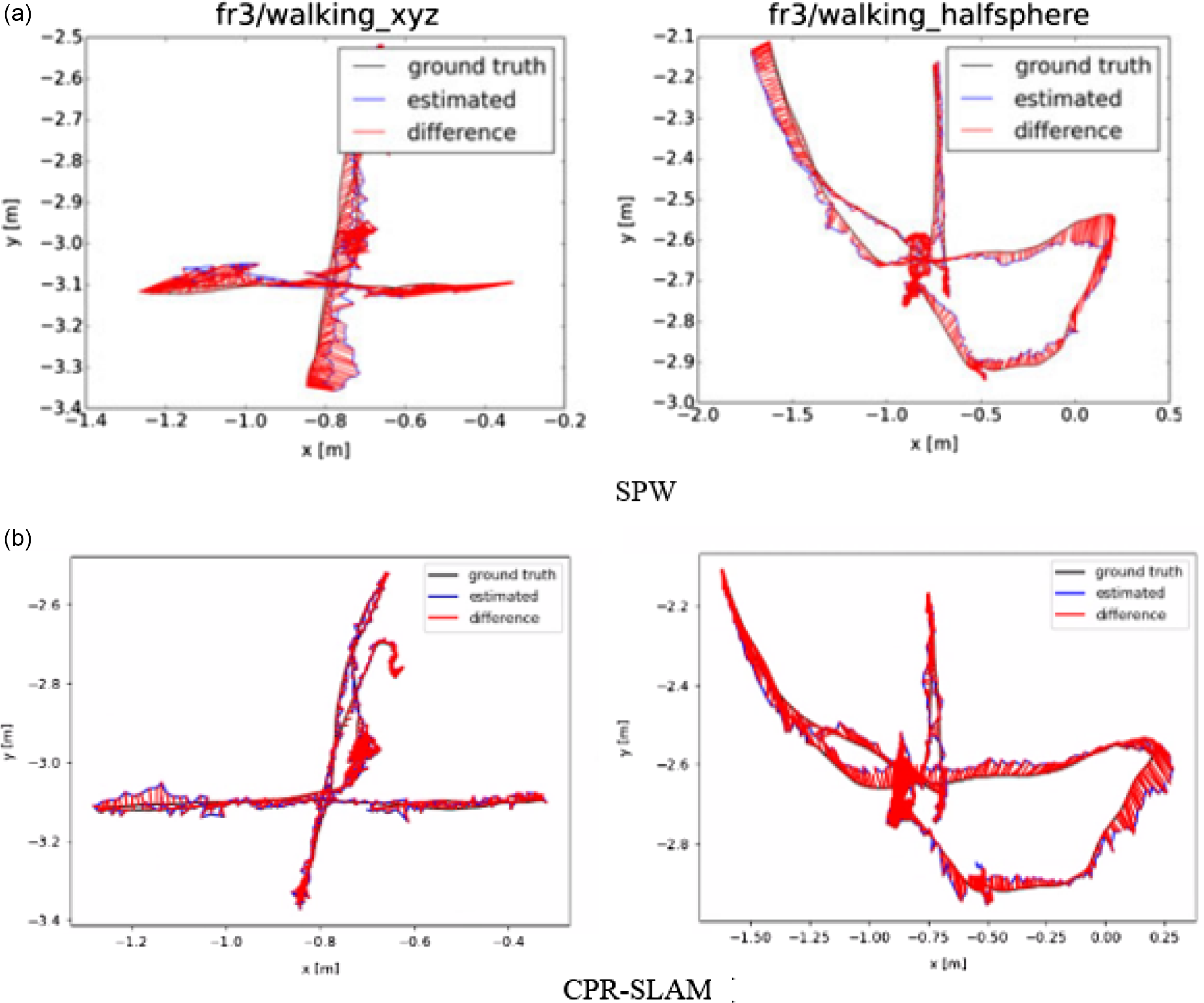
Figure 10. Comparison of the CPR-SLAM and SPW trajectory with the ground truth. The SPW result is from the original paper. The red line indicates the difference between the estimated trajectory and the ground truth. The shorter the red line, the more precise the estimated trajectory.
4.1.5. Performance of real environment
It is verified that the method proposed in this paper also has superior performance in the real environment. We will conduct the evaluation in two ways. Experiment A involves the camera being stationary, while Experiment B utilizes a OptriTrack pose capture device to obtain real-time robot poses.
4.5.1.1. Experiment A
In experiment A, the robot was kept stationary to observe the performance of the SLAM system, particularly whether it would erroneously identify itself as moving due to dynamic objects in the environment, leading to trajectory drift. What is more, we used the Realsense D455i depth camera as a sensor to design a scene in a real environment where a person dressed in black is walking casually indoors with a yellow doll. The recognition results of dynamic objects are shown in Fig. 11. In Fig. 11(b), a person is moving with a bear, and the upper limb is moving slowly. The dynamic module of the sub-point cloud can well identify the moving object without setting the prior information of the moving object in advance. The REMS of ATE of CPR-SLAM is 0.00299m. On the contrary, because ORBSLAM2 does not further process the dynamic object, the REMS of ATE is 0.05155m. In Fig. 11(a,c), it appears that the ground is also being recognized as a dynamic object. According to our analysis, this may be due to overfitting as a result of a fixed number of clusters. Anyway, the method proposed in this paper is an order of magnitude higher than the localization accuracy of ORBSLAM2.

Figure 11. Experiment A of RGB-D camera in real environment. Our method divides dynamic regions well. The first row is the tracking result of feature points, and the second row is the mask of dynamic regions.
4.5.1.2. Experiment B
In experiment B, we used the OptriTrack device to capture the real-time position of the robot, with the capture rate set at 30 Hz in this experiment. In the scene Fig. 12, a person is pushing a chair with a box while moving around, and the robot is performing irregular movements. The trajectory results for Experiment B are depicted below Fig. 13, where we will compare it with ORBSLAM2 and DynaSLAM [Reference Bescos, Fácil, Civera and Neira32]. As indicated in the legend, the black line represents the true trajectory captured by OptriTrack, the blue line represents the trajectory of ORBSLAM2, the green line represents the trajectory of our proposed method, and the red line represents the trajectory of DynaSLAM. It is evident that only the algorithm proposed in this paper maintains positioning accuracy within an acceptable range, while the other two exhibit varying degrees of drift. DynaSLAM, although also designed for dynamic environments, relies on deep learning and does not proactively label dynamic objects as such in the experiment. This inability to distinguish dynamic objects contributes to pose drift. Furthermore, this method is not real time, so in our experiment, the rosbag play rate was reduced to 0.3 times the original speed to allow DynaSLAM to process each frame as comprehensively as possible. On the contrary, CPR-SLAM demonstrates satisfactory performance in terms of both real-time processing and the recognition of both unknown and known dynamic objects.

Figure 12. Experiment B: a person is pushing a chair with a box while moving around.

Figure 13. Experiment B: the trajectory results.
5. Conclusion
In this paper,we proposed a dynamic VSLAM system CPR-SLAM based on ORBSLAM2. Our approach effectively segments dynamic areas by optimizing point cloud data to obtain sub-point clouds and introducing the concept of sub-poses. By combining the information from sub-point clouds and sub-poses, we successfully achieve the effective segmentation of dynamic areas. The proposed method yields satisfactory results on popular dynamic datasets. However, the processing of point cloud information in CPR-SLAM requires a substantial amount of computational resources and has redundant information, as shown in Table VI. Therefore, our future research will focus on reducing computational complexity by dimensionality reduction from three dimensions to two.
Table VI. The module runtime in the CPR-SLAM. Including sub-point cloud construction, correlation degree estimation, and keyframe refinement (ms).

Acknowledgments
This research was supported by the Baima Lake Laboratory Joint Funds of the Zhejiang Provincial Natural Science Foundation of China under Grant No. LBMHD24F030002 and the National Natural Science Foundation of China under Grant 62373329.
Author contributions
This study was jointly designed by the authors - Xinyi Yu and Wancai Zheng. Wancai Zheng conducted the data collection, development, and experiments, while Xinyi Yu and Linlin Ou participated in the evaluation. The article was written and organized by the author Wancai Zheng author under the guidance of Xinyi Yu and Linlin Ou.
Competing interests
The authors declare no competing interests.
Ethical standards
None.


