1. Diffuse interface models for two-phase flows
In recent years diffuse interface models for two- or multi-phase flows have generated an increasing interest because of theoretical developments as well as for their use in computations. In these models, macroscopically immiscible fluids are considered to be partly miscible and the Helmholtz free energy consists of a part which penalizes mixing, and gradient terms of the concentrations which enforce smooth transition regions between the fluids. This has the advantage that the interface does not need to be described explicitly in numerical simulations and one can describe flows beyond the occurrence of singularities in the interface due to the collision or pinch-off of droplets. A first diffuse interface model for two incompressible Newtonian fluids with same density  $\rho >0$ was given by Hohenberg & Halperin (Reference Hohenberg and Halperin1977). It is often called the ‘model H’ and leads to the following Navier–Stokes/Cahn–Hilliard system:
where we neglected exterior forces for simplicity. Here, $\boldsymbol {v}$ is a mean velocity of the fluid mixture, $\boldsymbol{\mathsf{D}}=\frac 12(\boldsymbol {\nabla } \boldsymbol {v}+\boldsymbol {\nabla } \boldsymbol {v}^{\rm T})$, $p$ is the pressure of the mixture and $c$ is difference of concentrations of the fluids. Moreover, $\nu =\nu (c)>0$ is the dynamic viscosity of the mixture, $\hat \sigma$ is a constant related to the surface energy density, $\varepsilon >0$ is a (small) parameter, which is related to the ‘thickness’ of the interfacial region (cf. figure 1), $\,f$ is a homogeneous free energy density, which has two strict minima at the values $\pm 1$ (or close to them), $\mu$ is the chemical potential of the mixture and $m>0$ is a mobility coefficient. A first derivation of this model in the framework of rational continuum mechanics was given by Gurtin, Polignone & Viñals (Reference Gurtin, Polignone and Viñals1996). Thermodynamically consistent extensions for fluids with different densities were given by Lowengrub & Truskinovsky (Reference Lowengrub and Truskinovsky1998), Abels, Garcke & Grün (Reference Abels, Garcke and Grün2012) and Aki et al. (Reference Aki, Dreyer, Giesselmann and Kraus2014). We note that these models differ in the choice of the mean velocity of the mixture, which is used for the conservation of linear momentum and the resulting constitutive assumptions. A unified approach to these kinds of diffuse interface models and comparison of these and other models were presented by ten Eikelder et al. (Reference ten Eikelder, van der Zee, Akkerman and Schillinger2023), where further references can be found. We remark that these models can be extended to diffuse interface models for more than two fluids. All these models lead to a system, where a Navier–Stokes-type equation for the chosen mean velocity of the mixture (similar to (1.1)–(1.2)) is coupled to a Cahn–Hilliard-type system (similar to (1.1)–(1.2)). The modelling is based on conservation laws for the conservation of mass of the individual components and the conservation of linear momentum for the mean velocity, while the momentum due relative motions of the fluids is neglected (cf. e.g. Gurtin et al. Reference Gurtin, Polignone and Viñals1996). Although terms and some basic ansatzes of mixture theories are used in the derivation, these models differ significantly from models derived by mixture theories, where a full set of conservation laws for each constituent is taken into account. Therefore these kinds of models are also called reduced mixture models (or class-I models in Bothe & Dreyer Reference Bothe and Dreyer2015). In (full) mixture models the conservation of linear momentum for each fluid of the mixture is considered. A derivation of diffuse interface models based on mixture theory for two- or multi-phase flow was missing for a long time. This gap was filled recently by ten Eikelder, van der Zee & Schillinger (Reference ten Eikelder, van der Zee and Schillinger2024). Some aspects of this will be summarized in the following.
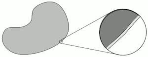
Figure 1. Schematic picture of a sharp interface resolved by a diffuse interface on small length scale $\varepsilon$ in a two-phase flow.
2. Link to mixture theory
ten Eikelder et al. (Reference ten Eikelder, van der Zee and Schillinger2024) give a rigorous derivation of a class of diffuse interface models for multi-phase flows of partly miscible incompressible fluids taking possible sources of mass for the individual fluids into account. In the following, we restrict ourselves for simplicity to the case of two fluids without mass sources. For a specific choice of a volume-measure-based Helmholtz free energy (denoted by ‘model I’) one obtains the following system of two coupled Navier–Stokes type equations:
Here, $\tilde {\rho }_\alpha = \rho _\alpha \phi _\alpha$ is the partial mass density of fluid $\alpha$, $\rho _\alpha >0$ is the specific density of fluid $\alpha$, $\phi _\alpha$ its volume fraction and $\mu _\alpha$ its chemical potential. Also, $\boldsymbol{\mathsf{D}}_\alpha$ is the symmetrized gradient of $\boldsymbol {v}_\alpha$, $\tilde {\nu }_\alpha$ and $\lambda _\alpha$ are the dynamic viscosity coefficient and second viscosity coefficient of fluid $\alpha$, $R_{12}=R_{21}>0$ is a coefficient for the rate of exchange of linear momentum between the fluids. One possible choice for the linear momentum exchange coefficient is given by the Stefan–Maxwell model
for some diffusion coefficient $D$. Here, $R>0$ is the gas constant (ten Eikelder et al. Reference ten Eikelder, van der Zee and Schillinger2024, Remark 3.10). Here, we neglected exterior forces for simplicity of the presentation. It is assumed that there is no excess volume due to mixing, i.e.
Finally, $p$ is a pressure allows to enforce the constraint (2.6). Dividing (2.3) by $\rho _\alpha$ and summation the equations for $\alpha =1,2$ yields
Here, $\phi _1\boldsymbol {v}_1 +\phi _2\boldsymbol {v}_2$ is the volume-averaged mean velocity used e.g. by Ding, Spelt & Shu (Reference Ding, Spelt and Shu2007) and Abels et al. (Reference Abels, Garcke and Grün2012). In the case of the same specific densities, $\rho _1=\rho _2$, the volume-averaged mean velocity coincides with the mass-averaged velocity used e.g. by Lowengrub & Truskinovsky (Reference Lowengrub and Truskinovsky1998) and the mean velocity $\boldsymbol {v}$ in the model H (1.1)–(1.4).
For the following, let $\boldsymbol {v}$ be the mass average (or barycentric) mean velocity defined by $\rho \boldsymbol {v}=\rho _1\boldsymbol {v}_1+\rho _2\boldsymbol {v}_2$. Because of (2.6), the conservation of masses (2.3) is equivalent to (2.7) and
where $\phi = \phi _1-\phi _2$ and $h= \phi _1\boldsymbol {v}_1-\phi _2\boldsymbol {v}_2-\phi \boldsymbol {v}$ is a diffusive flux for $\phi$, i.e. it is the flux of $\phi$ relative to the mean velocity $\boldsymbol {v}$ of the mixture. Here, the diffusive flux is related to a difference of velocities of the fluid, which are determined by solutions of two Navier–Stokes-type systems. In the case of the Navier–Stokes/Cahn–Hilliard system (1.1)–(1.4) one can divide (1.3) by the density $\rho$ and obtains for $\phi = {c}/\rho$
due to (1.2). Hence, the diffuse flux is given by $h=-({m}/\rho ) \boldsymbol {\nabla } \mu$, where $\mu$ is the chemical potential of the concentration difference. Similar relations also hold true for the diffuse interface models for different densities by Abels et al. (Reference Abels, Garcke and Grün2012), Lowengrub & Truskinovsky (Reference Lowengrub and Truskinovsky1998) and Aki et al. (Reference Aki, Dreyer, Giesselmann and Kraus2014) with the only difference that the pressure enters the definition of the chemical potential or flux in the latter two.
3. Remaining challenges
It remains an important task to understand to what extent solutions of the mixture model and the known diffuse interface model differ in practically relevant situations in numerical simulation. To this end suitable numerical methods have to be developed first. After that, a comparison of the efficiency of the numerical methods based on different models and a comparison with experiments are of great interest. Moreover, from the theoretical side it would be interesting to see how one could obtain a Navier–Stokes/Cahn–Hilliard model from the mixture theory model if one approximates (2.1)–(2.2) by a Navier–Stokes/Cahn–Hilliard model for the mean velocity $\boldsymbol {v}$ (ten Eikelder et al. Reference ten Eikelder, van der Zee and Schillinger2024, (5.66)) and a kind of Darcy law for $\phi _1\boldsymbol {v}_1-\phi _2\boldsymbol {v}_2-\phi \boldsymbol {v}$ for example based on a dimensional analysis. Finally, let us note that solutions of the Navier–Stokes/Cahn–Hilliard system (1.1)–(1.4) converge to a classical sharp interface model for the two-phase flow of incompressible fluids with a pure transport of the interface by the normal component of the fluid velocity only if $m\to 0$ as $\varepsilon \to 0$ (Abels et al. Reference Abels, Garcke and Grün2012, § 4), see also Abels, Fei & Moser (Reference Abels, Fei and Moser2024) for a recent mathematical result on that topic and further references. It might well be that, in situations where the mobility coefficient and the diffuse fluxes are small, the differences of the solutions of the different models (mixture model and the different Navier–Stokes/Cahn–Hilliard models) are negligible if applied with comparable parameters. Finally, the mathematical analysis of these new models concerning existence and properties of the solutions as well as the analysis of the sharp interface limit (formal and rigorous) are challenging open problems.


 $\varepsilon$ in a two-phase flow.
 You have
Access
You have
Access
 Open access
1. Diffuse interface models for two-phase flows
In recent years diffuse interface models for two- or multi-phase flows have generated an increasing interest because of theoretical developments as well as for their use in computations. In these models, macroscopically immiscible fluids are considered to be partly miscible and the Helmholtz free energy consists of a part which penalizes mixing, and gradient terms of the concentrations which enforce smooth transition regions between the fluids. This has the advantage that the interface does not need to be described explicitly in numerical simulations and one can describe flows beyond the occurrence of singularities in the interface due to the collision or pinch-off of droplets. A first diffuse interface model for two incompressible Newtonian fluids with same density $\rho >0$ was given by Hohenberg & Halperin (Reference Hohenberg and Halperin1977). It is often called the ‘model H’ and leads to the following Navier–Stokes/Cahn–Hilliard system:
where we neglected exterior forces for simplicity. Here, $\boldsymbol {v}$ is a mean velocity of the fluid mixture,
  $\boldsymbol{\mathsf{D}}=\frac 12(\boldsymbol {\nabla } \boldsymbol {v}+\boldsymbol {\nabla } \boldsymbol {v}^{\rm T})$,
  $p$ is the pressure of the mixture and
  $c$ is difference of concentrations of the fluids. Moreover,
  $\nu =\nu (c)>0$ is the dynamic viscosity of the mixture,
  $\hat \sigma$ is a constant related to the surface energy density,
  $\varepsilon >0$ is a (small) parameter, which is related to the ‘thickness’ of the interfacial region (cf. figure 1),
  $\,f$ is a homogeneous free energy density, which has two strict minima at the values
  $\pm 1$ (or close to them),
  $\mu$ is the chemical potential of the mixture and
  $m>0$ is a mobility coefficient. A first derivation of this model in the framework of rational continuum mechanics was given by Gurtin, Polignone & Viñals (Reference Gurtin, Polignone and Viñals1996). Thermodynamically consistent extensions for fluids with different densities were given by Lowengrub & Truskinovsky (Reference Lowengrub and Truskinovsky1998), Abels, Garcke & Grün (Reference Abels, Garcke and Grün2012) and Aki et al. (Reference Aki, Dreyer, Giesselmann and Kraus2014). We note that these models differ in the choice of the mean velocity of the mixture, which is used for the conservation of linear momentum and the resulting constitutive assumptions. A unified approach to these kinds of diffuse interface models and comparison of these and other models were presented by ten Eikelder et al. (Reference ten Eikelder, van der Zee, Akkerman and Schillinger2023), where further references can be found. We remark that these models can be extended to diffuse interface models for more than two fluids. All these models lead to a system, where a Navier–Stokes-type equation for the chosen mean velocity of the mixture (similar to (1.1)–(1.2)) is coupled to a Cahn–Hilliard-type system (similar to (1.1)–(1.2)). The modelling is based on conservation laws for the conservation of mass of the individual components and the conservation of linear momentum for the mean velocity, while the momentum due relative motions of the fluids is neglected (cf. e.g. Gurtin et al. Reference Gurtin, Polignone and Viñals1996). Although terms and some basic ansatzes of mixture theories are used in the derivation, these models differ significantly from models derived by mixture theories, where a full set of conservation laws for each constituent is taken into account. Therefore these kinds of models are also called reduced mixture models (or class-I models in Bothe & Dreyer Reference Bothe and Dreyer2015). In (full) mixture models the conservation of linear momentum for each fluid of the mixture is considered. A derivation of diffuse interface models based on mixture theory for two- or multi-phase flow was missing for a long time. This gap was filled recently by ten Eikelder, van der Zee & Schillinger (Reference ten Eikelder, van der Zee and Schillinger2024). Some aspects of this will be summarized in the following.
Figure 1. Schematic picture of a sharp interface resolved by a diffuse interface on small length scale $\varepsilon$ in a two-phase flow.
2. Link to mixture theory
ten Eikelder et al. (Reference ten Eikelder, van der Zee and Schillinger2024) give a rigorous derivation of a class of diffuse interface models for multi-phase flows of partly miscible incompressible fluids taking possible sources of mass for the individual fluids into account. In the following, we restrict ourselves for simplicity to the case of two fluids without mass sources. For a specific choice of a volume-measure-based Helmholtz free energy (denoted by ‘model I’) one obtains the following system of two coupled Navier–Stokes type equations:
Here, $\tilde {\rho }_\alpha = \rho _\alpha \phi _\alpha$ is the partial mass density of fluid
  $\alpha$,
  $\rho _\alpha >0$ is the specific density of fluid
  $\alpha$,
  $\phi _\alpha$ its volume fraction and
  $\mu _\alpha$ its chemical potential. Also,
  $\boldsymbol{\mathsf{D}}_\alpha$ is the symmetrized gradient of
  $\boldsymbol {v}_\alpha$,
  $\tilde {\nu }_\alpha$ and
  $\lambda _\alpha$ are the dynamic viscosity coefficient and second viscosity coefficient of fluid
  $\alpha$,
  $R_{12}=R_{21}>0$ is a coefficient for the rate of exchange of linear momentum between the fluids. One possible choice for the linear momentum exchange coefficient is given by the Stefan–Maxwell model
for some diffusion coefficient $D$. Here,
  $R>0$ is the gas constant (ten Eikelder et al. Reference ten Eikelder, van der Zee and Schillinger2024, Remark 3.10). Here, we neglected exterior forces for simplicity of the presentation. It is assumed that there is no excess volume due to mixing, i.e.
Finally, $p$ is a pressure allows to enforce the constraint (2.6). Dividing (2.3) by
  $\rho _\alpha$ and summation the equations for
  $\alpha =1,2$ yields
Here, $\phi _1\boldsymbol {v}_1 +\phi _2\boldsymbol {v}_2$ is the volume-averaged mean velocity used e.g. by Ding, Spelt & Shu (Reference Ding, Spelt and Shu2007) and Abels et al. (Reference Abels, Garcke and Grün2012). In the case of the same specific densities,
  $\rho _1=\rho _2$, the volume-averaged mean velocity coincides with the mass-averaged velocity used e.g. by Lowengrub & Truskinovsky (Reference Lowengrub and Truskinovsky1998) and the mean velocity
  $\boldsymbol {v}$ in the model H (1.1)–(1.4).
For the following, let $\boldsymbol {v}$ be the mass average (or barycentric) mean velocity defined by
  $\rho \boldsymbol {v}=\rho _1\boldsymbol {v}_1+\rho _2\boldsymbol {v}_2$. Because of (2.6), the conservation of masses (2.3) is equivalent to (2.7) and
where $\phi = \phi _1-\phi _2$ and
  $h= \phi _1\boldsymbol {v}_1-\phi _2\boldsymbol {v}_2-\phi \boldsymbol {v}$ is a diffusive flux for
  $\phi$, i.e. it is the flux of
  $\phi$ relative to the mean velocity
  $\boldsymbol {v}$ of the mixture. Here, the diffusive flux is related to a difference of velocities of the fluid, which are determined by solutions of two Navier–Stokes-type systems. In the case of the Navier–Stokes/Cahn–Hilliard system (1.1)–(1.4) one can divide (1.3) by the density
  $\rho$ and obtains for
  $\phi = {c}/\rho$
due to (1.2). Hence, the diffuse flux is given by $h=-({m}/\rho ) \boldsymbol {\nabla } \mu$, where
  $\mu$ is the chemical potential of the concentration difference. Similar relations also hold true for the diffuse interface models for different densities by Abels et al. (Reference Abels, Garcke and Grün2012), Lowengrub & Truskinovsky (Reference Lowengrub and Truskinovsky1998) and Aki et al. (Reference Aki, Dreyer, Giesselmann and Kraus2014) with the only difference that the pressure enters the definition of the chemical potential or flux in the latter two.
3. Remaining challenges
It remains an important task to understand to what extent solutions of the mixture model and the known diffuse interface model differ in practically relevant situations in numerical simulation. To this end suitable numerical methods have to be developed first. After that, a comparison of the efficiency of the numerical methods based on different models and a comparison with experiments are of great interest. Moreover, from the theoretical side it would be interesting to see how one could obtain a Navier–Stokes/Cahn–Hilliard model from the mixture theory model if one approximates (2.1)–(2.2) by a Navier–Stokes/Cahn–Hilliard model for the mean velocity $\boldsymbol {v}$ (ten Eikelder et al. Reference ten Eikelder, van der Zee and Schillinger2024, (5.66)) and a kind of Darcy law for
  $\phi _1\boldsymbol {v}_1-\phi _2\boldsymbol {v}_2-\phi \boldsymbol {v}$ for example based on a dimensional analysis. Finally, let us note that solutions of the Navier–Stokes/Cahn–Hilliard system (1.1)–(1.4) converge to a classical sharp interface model for the two-phase flow of incompressible fluids with a pure transport of the interface by the normal component of the fluid velocity only if
  $m\to 0$ as
  $\varepsilon \to 0$ (Abels et al. Reference Abels, Garcke and Grün2012, § 4), see also Abels, Fei & Moser (Reference Abels, Fei and Moser2024) for a recent mathematical result on that topic and further references. It might well be that, in situations where the mobility coefficient and the diffuse fluxes are small, the differences of the solutions of the different models (mixture model and the different Navier–Stokes/Cahn–Hilliard models) are negligible if applied with comparable parameters. Finally, the mathematical analysis of these new models concerning existence and properties of the solutions as well as the analysis of the sharp interface limit (formal and rigorous) are challenging open problems.
Declaration of interests
The author reports no conflict of interest.