INTRODUCTION
Influenza is an acute contagious disease caused by a virus [1]. There are three types of the virus, designated A, B, and C, but only types A and B cause more serious contagious infections. Influenza occurs most often in late autumn, winter and early spring, and it usually reaches peak prevalence in winter. It is a serious infection, afflicting millions of people throughout the world every year. Therefore, it is very important to have a good model describing influenza's behaviour and giving reliable predictions. Even though influenza cases are count data they exhibit time-series properties. In this paper we use a time-series approach to model data on the weekly incidence of human influenza A cases in England and Wales in 1992–2005 [2].
Many authors have used a time-series approach to model infectious diseases. Choi & Thacker [Reference Choi and Thacker3, Reference Choi and Thacker4] proposed the ARIMA model for forecasting the expected mortality and the percentage of pneumonia and influenza death. Quénel & Dab [Reference Quénel and Dab5] modelled the weekly influenza incidences in France by a SARIMA model. They developed epidemic criteria based on time-series analysis. A time-series analysis approach was also used by Crighton et al. [Reference Crighton6]. Their main concern was the gender- and age-specific influenza and pneumonia hospitalization seasonality. Mugglin et al. [Reference Mugglin, Cressie and Gemmell7] used a Bayesian hierarchical approach for modelling of influenza epidemic dynamics in both time and space, while Cliff & Hagget [Reference Cliff and Haggett8] give a review of applications of statistical models to outbreaks of (measles and) influenza.
We propose to model the weekly influenza incidences by a Gaussian random process with a seasonal variance. In a good time-series model, residuals obtained after removing deterministic components should be randomly distributed, exhibit a normal distribution, have non-significant autocorrelations and partial autocorrelations, and have a mean of zero and homogeneous variance over time. However, some financial and meteorological applications [Reference Benth and Šaltytė-Benth9, Reference Šaltytė Benth, Benth and Jalinskas10] clearly indicate that even though the final residuals of a time-series model fulfil those requirements, the analysis of squared residuals and their autocorrelation function often show the presence of seasonal effects. We can improve the model quality and prediction reliability by detecting and modelling such effects by relatively simple methods. Kakehashi et al. [Reference Kakehashi11] use a somewhat similar approach for modelling monthly influenza (and measles) time-series from Japan. They decompose the time-series into a seasonal component presented as seasonal indices, a (quadratic) trend and an AR(1) process. Their model fits the data well. They also present an attractive TS-decomposition diagram. This paper aims to show that relatively simple additional analyses of the residuals can improve the modelling.
The remainder of the paper is divided into five sections. First, we present a detailed description of the English and Welsh influenza incidence data. Next, we perform a simple statistical analysis to explore the data and generate some ideas for a possible model. Third, we present a time-series model and estimate the proposed model on the basis of in-sample data. Fourth, the out-of-sample data are used for the validation of the model. Here we also demonstrate how the proposed model can be used for the prediction of influenza incidence. In the last section we summarize the results.
Data were analysed by Excel (Microsoft, Redmond, WA, USA), SPSS (SPSS Inc., Chicago, IL, USA), and Matlab (MathWorks Inc., Natick, MA, USA).
DATA
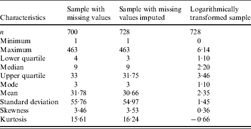
Our data source is the routine influenza laboratory reports from hospitals in England and Wales [2], representing influenza A cases registered in England and Wales in the period from the beginning of 1992 to the end of 2005 by week per 100 000. The total length of the series is 728 weekly observations. Observations are missing for 28 weeks (3·8%). The years 1992, 1998, and 2005 had 53 weeks, with the 53rd week having 1, 221 and 6 cases, respectively. To avoid problems with periodicity, we merged the observations from weeks 53 of 1992 and 2005 with the observation in week 52 in the corresponding year. We split the 221 observations from week 53 of 1998 into two parts: 110 to week 52 in 1998 and the rest (111) to week 1 of 1999. The 28 missing values were substituted with the mean of two nearby points. A number of descriptive statistic characteristics for the sample with missing values and the sample with imputed missing values are presented in Table 1 (columns 2 and 3), showing that the two datasets are nearly identical; their means and variances were not significantly different, neither were the 95% confidence intervals for skewness and kurtosis. We also tried a number of other substitution methods; however, variations in descriptive characteristics were only minor. Thus, we have 728 valid observations, which we plot in Figure 1 and their logarithm in Figure 2.
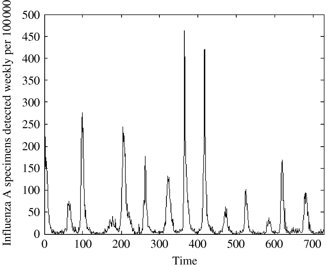
Fig. 1. Influenza A specimens detected in England and Wales from 1992–2005 by week per 100 000.
Table 1. Descriptive statistic characteristics for sample with missing values, sample with missing values imputed, and the logarithmically transformed data
We see from Figure 1, that influenza peaks differ in size but the peaks appear in a quite regular manner, corresponding to the influenza season, which usually lasts from week 40 to week 20. Note that the variation is season-dependent, higher in a cold season and lower in a warm one. Figure 3 shows that the distribution is strongly left-skewed. It indicates clear presence of extremes; there are years with very high peaks, e.g. in week 1 there were peaks in two years (463 cases/100 000 in 1999 and 419 cases/100 000 in 2000).
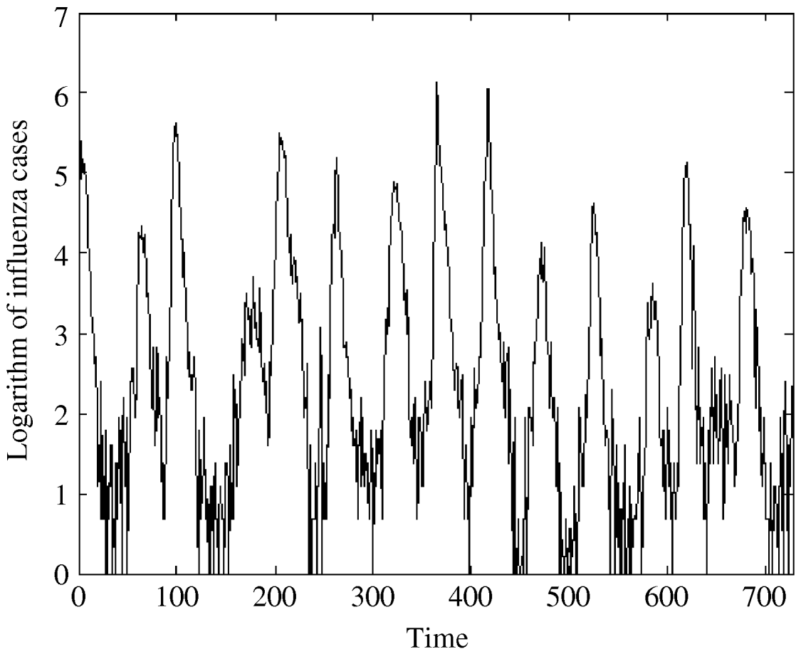
Fig. 2. The logarithm of influenza A specimens detected in England and Wales from 1992–2005 by week per 100 000.

Fig. 3. Frequency of influenza cases.
In the autocorrelation function (ACF) of influenza cases (Fig. 4a), we also observe strong seasonal effects and significant autocorrelations: the autocorrelation values are far beyond the 95% confidence intervals.
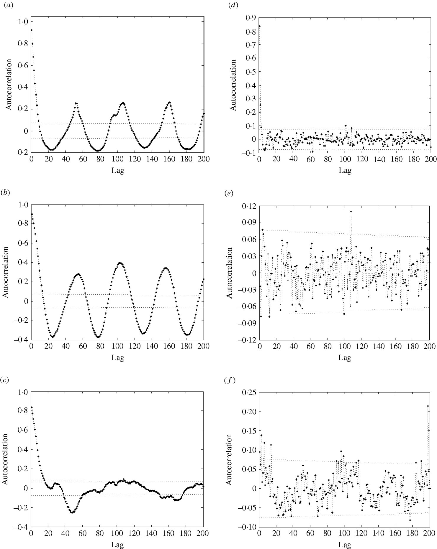
Fig. 4. Autocorrelation function (ACF) (with 95% confidence intervals) of (a) influenza cases; (b) logarithm of influenza cases; (c) residuals after trend and seasonal effects were eliminated; (d) partial ACF of residuals after trend and seasonal effects were eliminated; (e) ACF of residuals after removal of trend, seasonal effects, and AR(2) process; (f) ACF of squared residuals after removal of trend, seasonal effects, and AR(2) process.
The regression analysis of influenza observations and logarithmically transformed influenza observations on time resulted in higher R 2 value for logarithmically transformed data. The logarithmic transformation also symmetrized the distribution of the considered data; skewness, even though significant, is close to zero for transformed data. The kurtosis of the distribution does not differ significantly from zero. Therefore, we choose to use logarithmically transformed time-series. We still observe strong seasonal variations in the transformed series (Fig. 2). Moreover, the ACF (Fig. 4b) preserves the pattern observed for the original data. It should be noted that the logarithmical transformation was possible since the minimum count in the original series was 1.
Before defining the model for influenza observations, we shall briefly describe the modelling idea. As more people than before may be vaccinated against influenza one might expect a decrease in the frequency of influenza cases. Therefore, a first step in the data analysis would be to check for the presence of a trend. As can be seen in Figures 1 and 2 it is obvious that influenza has a clear seasonal pattern. We model such seasonal variations with a simple cosine function.
Usually the frequency of infections falls after certain peak is reached. Therefore, we include the autoregressive (AR) process in the model as well. The partial ACF (PACF) will be used to define the order of the AR process.
We eliminated those components from the data step by step. First, we detrended and deseasonalized the influenza observations. We then applied the AR process to the resulting data and checked whether the residuals were uncorrelated and normally distributed. As will be shown later, a more complicated model for residuals was needed.
We estimated the proposed model on the basis of the in-sample data, which consisted of observations from the period 1992–2004 (676 observations). For validation of the proposed model we used the data from 2005 (out-of-sample data).
MODEL
In this section we define our model for the influenza observations.
We denote by X(t) the number of influenza incidences observed at the time moment t∊[0, ∞). We decomposed – as this is a standard procedure – X(t) into a mean component μ(t), modelling the trend, and a residual component ε(t), modelling the fluctuations around the trend in time:
the mean μ(t) is given by
where S(t) is a deterministic seasonal function of time given by
with level a 0, linear trend slope a 1, amplitude a 2 and time shift a 3. The function S(t) describes the (linear) trend and the seasonality in data. One might also consider the higher order (e.g. quadratic) trend; however, the second-order function implies problems with extrapolation for out-of-sample data. The coefficient αk (k=1, …, p), is a parameter of the AR process of order p (AR(p)).
The residuals of a model that fits the data well should be a white noise. However, experience shows that this is often not the case, i.e. we may need to factorize the residual process into
where σ(t) is a non-random (possibly) seasonal function. Assume that {δ(t): t∊[0, ∞)} is a zero-mean stationary Gaussian random process, which is independent in time, or white noise. If the ACF of the squared residuals exhibits seasonal variation, one can model them in many different ways. One could use for instance the following (rather general) function
It might also be that the empirical variance or the average variance can simply be enough to obtain the white-noise residuals. In the next section we fit the suggested model to the in-sample influenza data and choose an appropriate model for the variance of residuals. This additional step in the analysis helps us to obtain the residuals, which are more or less white noise.
Model fitting
First, we checked for linear trend in the considered dataset, by simply regressing influenza cases on the time variable. Intercept (2·728) and slope (−0·001) values were both significant at the 1% level. This presence of linear trend basically means that the average number of influenza cases has decreased by 0·67 on a logarithmic scale, which corresponds to a decrease of about 1·96 cases/100 000 per week.
In the proposed model, the linear trend and seasonal component were estimated simultaneously. The parameters of function S(t) were fitted using the nlinfit procedure in Matlab. All estimates were significant at the 5% level and are reported in Table 2 (columns 1–4). The function S(t) fits the data reasonably well, with R 2=42%.
Table 2. Estimates of parameters of the seasonal function, the AR(2) process and the seasonal variance function

We then eliminated the trend and seasonal effects from the data and evaluated the properties of the resulting residuals. The residuals were normally distributed [P value=0·918 for the Kolmogorov–Smirnov (KS) test]; however, we still observed strong significant autocorrelations (Fig. 4c). Admittedly, the P value should be treated with care since the KS test is designed for use with independent observations.
The PACF plot in Figure 4d clearly indicated a need for – at least – an AR(2) process to explain the remaining variation in the residuals. The parameters of the AR(2) process (Table 2, columns 5 and 6) were both significant at the 1% level. Naturally, the constant of the AR(2) process was insignificant and therefore excluded from the model. We modelled the process both as AR(2) and AR(3). The AR(3) process gave a better fit, however, the differences in the values of coefficients were not great, and the mean square error (MSE) differed by only <1%. Therefore, we chose to model the data with an AR(2) process.
After the AR(2) process was fitted and eliminated, residuals were close to normal (P=0·046 for KS test) and not autocorrelated (see Fig. 4e) according to the Box–Ljung test. Now the value of R 2 has increased to 83%, indicating a good model fit.
As the ACF of the residuals is often insufficient to check if all seasonal effects are removed, we plotted the ACF of the squared residuals (Fig. 4f). As that plot shows, the residuals still exhibit seasonal variation, which should be modelled. The residuals contain a seasonal component σ(t)=σ(t+52), which we suggest to be modelled in the following way. We calculated the weekly empirical variance by averaging the values of the squared residuals of the particular week over all years. Then we modelled it by the function (1). First, we fitted a function with nine parameters; however, most of the parameters were not significantly different from zero. We concluded that the following function with only two parameters describes well the seasonal behaviour of the variance:
The fitted parameters of this function are presented in Table 2 (columns 7 and 8). For comparison, we also used both the empirical weekly and the average empirical variance in the model for the considered time-series. The three variance functions are plotted in Figure 5.
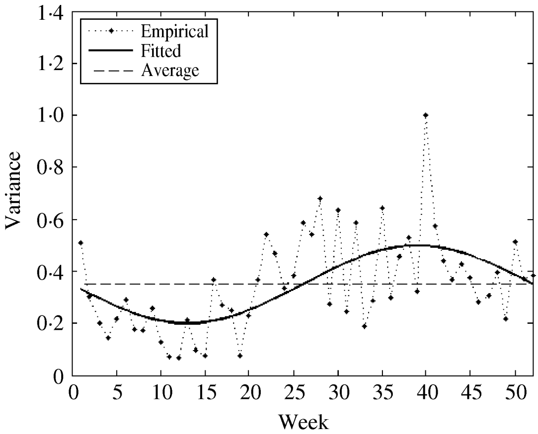
Fig. 5. The empirical, constant (average), and fitted variance functions.
We observed that variations in the cold season are considerably higher than those in the warm season. This could possibly be explained by the low number of influenza cases in the warm season.
We simulated 20 paths for each considered variance function. The averages of the obtained mean square simulation errors (MSSE) are presented in Table 3. As expected, the smallest MSSE was obtained for the fitted seasonal variance. In addition, we simulated the path under the assumption that the residuals obtained after eliminating trend, seasonal component and AR process, are white noise. The MSSE in this case was more than double that of the other MSSEs.
Table 3. The average of three mean square simulation errors (MSSEs) for considered variance functions

The ACFs of the final residuals for three considered variance functions are shown in Figure 6(a–c). All three plots show that the residuals are not autocorrelated – as is confirmed by the non-significant Box–Ljung statistics. Moreover, they are normally distributed with an average around zero and a standard deviation (s.d.) around 1 (see Table 4). The hypothesis about the homogeneity of weekly variances was not rejected for the seasonal and empirical variance functions while for the constant variance function the homogeneity assumption was strongly violated (Levene's test statistic was significant at the 1% level). The ACFs for squared residuals (Fig. 6d–f) clearly reflects the fact that seasonal variance is still present in the case of the constant variance model. This illustrates the importance of seasonal variance function in the model.

Fig. 6. Autocorrelation function (with 95% confidence intervals) of (a) final residuals for fitted seasonal variance; (b) final residuals for empirical variance; (c) final residuals for average variance; (d) squared final residuals for fitted seasonal variance; (e) squared final residuals for empirical variance; (f) squared final residuals for average variance.
Table 4. Descriptive statistics and P values for the Kolmogorov–Smirnov test for residuals

The residuals from the model with seasonal variance function have all the properties of a good model. The next step is the validation of the suggested model on the basis of the out-of-sample observations.
Model validation and prediction
We used 52 out-of-sample observations from 2005 for model validation. To validate the model, we generated the one-week-ahead predictions for out-of-sample observations. The prediction errors (the differences between the observations and the predictions) turned out to be normally distributed (P value=0·708 for KS test) with a mean value of −0·123 and a standard deviation of 0·666, and not autocorrelated. Figure 7 shows the observed and predicted values for the out-of-sample period with bands of 2 s.d. from the prediction (Fig. 7, solid line). The standard deviation is calculated from the fitted variance function for each time-point. Only 8·0% of observations were beyond these bands. For comparison, we drew the corresponding bands for the empirical and average variances. In the case of the empirical variance, 12% of all observations were beyond the 2 s.d. interval. The corresponding number for the case of average variance was 8%. The proposed model had no observations beyond the 3 s.d. interval, while 4% and 2% of observations were outside the interval of 3 s.d. for the cases of empirical and constant variances, respectively. Bearing in mind the residuals analysis, we conclude that the considered model performs well and therefore can generate reliable predictions.

Fig. 7. Out-of-sample data and prediction with two standard deviation intervals. —, Fitted variance function; – – –, empirical variance; · · · · · , average variance.
We based the model validation on the prediction. The one-week-ahead prediction was obtained from the following equation:
The three-weeks-ahead prediction, then, would be as follows:
and so on.
DISCUSSION
In the paper we present a rather simple model, which fits well the weekly influenza incidence data from England and Wales. A quite standard way to analyse seasonally varying time-series is decomposing them into a seasonal component, a trend and an AR process. The residuals obtained after eliminating these components often do not reveal time dependency and come from normal or close to normal distribution. We suggest that conclusions should not be drawn only on the basis of residuals and that one should consider one more step – the analysis of squared residuals.
We show that squared residuals can reveal the presence of the remaining seasonal variation, which is not exhibited by the analysis of residuals. The modelling of such seasonal variations undoubtedly improves model fit. In our paper we model the seasonal variance with a simple trigonometric function. Although our method for estimating the variance function may look somewhat ad hoc, it clearly demonstrates the seasonality of data. Once the shape of σ2(t) becomes known, one can implement the maximum likelihood estimation procedure. In the case of time-dependent residuals the weighted regression [Reference Carroll and Ruppert12] or even iteratively weighted regression [Reference Hayman13] can be performed.
The proposed model can relatively easily be generalized to the spatial case by choosing the best-fitting spatial correlation function and incorporating it into the model. However, we had only aggregated data available.
There is an increasing concern about a human pandemic strain of influenza A. Our model is not intended to model the pandemic data. It is difficult to assess such a model without the data. However, the model with a stochastic regime-switching component, where specification of parameters is set by the opinion of experts, could be a reasonable choice.
ACKNOWLEDGEMENTS
We are grateful to the Health Protection Agency, UK, for providing us with data. We thank Fred Espen Benth for inspiring discussions.
DECLARATION OF INTEREST
None.


