


1. Introduction
Mobile robots are being increasingly deployed across a wide range of applications [Reference Alatise and Hancke1, Reference Delmerico, Mintchev, Giusti, Gromov, Melo, Horvat, Cadena, Hutter, Ijspeert, Floreano, Gambardella, Siegwart and Scaramuzza2], such as search and rescue operations, hospital services, and office deliveries. In these scenarios, the robots are required to autonomously navigate and explore unknown environments in order to gather information and efficiently accomplish their tasks. For instance, search and rescue robots must rapidly and autonomously search through disaster-stricken areas, while hospital service and office delivery robots need to efficiently explore and map large and complex environments without the need for additional human intervention. Therefore, the autonomously exploration and navigation through unknown environments represent critical capabilities for mobile robots.

Figure 1. Overview of our method. The example environment which the robot is required to explore is shown as a 2D map. Explored areas are depicted in blue, while unexplored regions are represented by white spaces. Our method comprises two stages: the exploration stage and the relocation stage. During the exploration stage, an Rapidly-exploring Random Tree is expanded within the local planning horizon, where each node serves as a viewpoint. Frontiers are identified from these viewpoints. The identified local frontiers are considered as possible exploration goals. They are clustered, with each cluster corresponding to a local navigation goal candidate. By using local tour planning, the optimal local navigation goal is selected for execution, considering the remaining goals as possible global exploration goals. Once no clusters in the local planning horizon remain, the robot switches to the relocation stage. In this stage, all updated global exploration goals are clustered and employed for global tour planning. The robot is then guided toward the selected global navigation goal. These two stages are executed back and forth until no global exploration goals remain.
Conventional exploration methods typically involve detecting frontiers [Reference Sun, Wu, Xu and Kong3, Reference Yamauchi4], sampling viewpoints, and navigating the robot toward the viewpoint with the highest information gain. These methods often rely on either frontiers or randomly sampled viewpoints. Frontiers are special locations that separate explored areas from unexplored ones and were first introduced for autonomous exploration by Yamauchi et al. [Reference Yamauchi4]. However, the challenge remains in how to detect frontiers and select optimal frontiers for exploration to maximize navigation efficiency and area coverage. On the other hand, most viewpoint-based approaches tend to be greedy, with viewpoints densely sampled around the robot and maintained throughout the exploration process. Without proper tour planning, the robot may spend considerable time navigating back to viewpoints that are close to already explored regions. Therefore, both frontier-based and viewpoint-based exploration methods frequently encounter challenges such as relying exclusively on information gain [Reference Liu, Wang, Chi, Chen and Sun5] for the selection of navigation goals and not optimizing the exploration path effectively. This leads to reduced efficiency in exploration, particularly in highly convoluted environments. Recent reinforcement learning-based methods [Reference Hu, Niu, Carrasco, Lennox and Arvin6–Reference Xu, Yu, Tang, Qiu, Wang, Shen, Wang and Yang8] focus on learning exploration policies and do not consider full area coverage. The performance cannot be guaranteed when transferring learned policy to new environments.
In this paper, we propose a dual-stage exploration method that combines spatial clustering and tour planning to address these challenges. Instead of individually assessing the information gained for each potential exploration goal, spatially clustering all possible densely distributed exploration goals allows the robot to rapidly determine sparse navigation goals. Tour planning based on Traveling Salesman Problem (TSP) framework is executed on these sparse navigation goals, optimizing the robot’s path by considering place-to-place costs and reducing computation load by limiting the number of tour locations. Spatial clustering and tour planning are performed on both local and global scales.
Fig. 1 offers an overview of our method. During the exploration stage, frontiers are identified from an Rapidly-exploring Random Tree (RRT) without any bias, all within the local planning horizon. These frontiers are always densely distributed and considered as possible local exploration goals. They are subsequently clustered and transformed into individual local navigation goal candidates. Planning tours based on the local navigation goal candidates and the robot’s home position allows for the rapid expansion of the exploration boundary. When no local exploration goal clusters remain, the robot transitions to the relocation stage. Our method again clusters all possible global exploration goals that have not been visited before and perform global tour planning. This empowers the robot to optimally navigate to different recognized but unexplored sub-areas. These two stages are repeated until no global exploration goals remain. In addition, a retrying mechanism is introduced to employ before the robot switches to the relocation stage from the exploration stage, in order to enhance the exploration robustness.
1.1. Contributions
Our contributions can be summarized as follows:
-
We propose to combine spatial clustering and TSP-based tour planning technologies in both exploration and relocation stages.
-
A retrying mechanism is suggested to enhance the robustness of exploration.
-
Our code is open-source, allowing others to reproduce our results and conduct comparative analyses with various exploration techniques.
2. Related work
Autonomous exploration of unknown environments has been extensively investigated in mobile robots, ranging from unmanned ground vehicle [Reference Umari and Mukhopadhyay9–Reference Zhu, Cao, Xia, Scherer, Zhang and Wang11] to unmanned aerial vehicle [Reference Dai, Papatheodorou, Funk, Tzoumanikas and Leutenegger12, Reference Zhou, Zhang, Chen and Shen13], and others. The exploration task can be executed either by a single-robot or in a multi-robot configuration [Reference Bi, Zhang, Wen, Pan, Zhang, Wang and Yuan14–Reference Soni, Dasannacharya, Gautam, Shekhawat and Mohan16]. Typically, these methods can be categorized into two groups: traditional approaches and machine learning-based techniques. Traditional methods mainly rely on frontiers and viewpoints, employing a greedy strategy for exploring unknown environments. Most traditional techniques ensure completeness by guaranteeing full space coverage [Reference Umari and Mukhopadhyay9]. In contrast, machine learning-based methods [Reference Hu, Niu, Carrasco, Lennox and Arvin6, Reference Xu, Yu, Tang, Qiu, Wang, Shen, Wang and Yang8] may not offer completeness, and the performance cannot always be guaranteed when transferring learned policy to new environments.
The central challenge in frontier-based exploration lies in frontier detection and selection. Typically, frontiers are identified as centroids of frontier edges, which are the lines separating known from the unknown space [Reference Yamauchi4]. One approach to detecting frontiers [Reference Umari and Mukhopadhyay9] involves expanding an RRT [Reference LaValle17] until its nodes extend into the unknown region of the map. Nodes within the unknown region are then considered as frontiers. To speed up the search for frontiers, multiple independently growing trees are utilized. In ref. [Reference Sun, Wu, Xu and Kong3], an adaptive frontier detection method is proposed to enhance the successful sampling rate of RRT and solve the oversampling issue of RRT in sliding windows. Once frontiers are detected, a simple policy for selecting navigation goals is to choose the nearest frontier as the exploration target. Another policy involves selecting frontiers by minimizing map entropy concerning occupancy probabilities [Reference Wang, Chi, Sun and Meng10, Reference Dai, Papatheodorou, Funk, Tzoumanikas and Leutenegger12]. Instead of choosing a single frontier, some works [Reference Meng, Qin, Chen, Chen, Sun, Lin and Ang18] exploit all frontiers and employ tour planning to determine the sequence for visiting all frontiers. However, as the number of frontiers increases, the computation load of tour planner escalates.
Viewpoint-based exploration methods focus on the generation of viewpoints and the calculation of their exploration gain. The “Next-Best-View” Planner (NBVP) [Reference Bircher, Kamel, Alexis, Oleynikova and Siegwart19] is a well-known method that treats nodes in the RRT as viewpoints, assessing their exploration gain based on the number of unknown voxels observed from each viewpoint. The robot then plans its path toward the viewpoint with the highest gain. Another approach is the Graph-Based Exploration Planner (GBP) [Reference Dang, Tranzatto, Khattak, Mascarich, Alexis and Hutter20], which constructs a global rapidly exploring random graph to guide the robot toward unexplored spaces. The Dual-Stage Viewpoint Planner (DSVP) method [Reference Zhu, Cao, Xia, Scherer, Zhang and Wang11] draws ideas from both frontier-based and viewpoint-based methods. DSVP employs local frontiers to guide the expansion of a RRT, where each node serves as a candidate viewpoint. It also utilizes global frontiers to relocate the robot to different sub-areas. The approach comprises two stages: an exploration stage for expanding the exploration boundary and a relocation stage for revisiting unexplored sub-areas. During the exploration stage, each RRT node serves as a viewpoint, and the RRT branch with the highest gain is employed for exploration. When no local frontiers remain, the robot switches to the relocation state and is directed to different areas based on global frontiers. DSVP has shown great performance across various unknown environments. In ref. [Reference Zhou, Zhang, Chen and Shen13], viewpoints capable of covering local frontier clusters are generated, and a tour planner is employed to determine the optimal sequence for visiting these viewpoints. The tour planner operates on a small scale, ensuring computational efficiency. In ref. [Reference Huang, Zhou, Fan, Zhu, Jie, Li and Cheng21], a rapid autonomous exploration method (FAEL) is introduced, taking into account factors such as information gain, movement distance, and coverage efficiency simultaneously. However, it falls short of ensuring complete space coverage. Furthermore, it does not address the requirement of returning to a home position, which is crucial in many scenarios, especially those with only one exit.
Inspired by the DSVP method, our work follows the dual-stage framework. We propose to combine spatial clustering and TSP-based tour planning technologies for efficient exploration in both stages. Through extensive experiments in a variety of highly convoluted environments, we demonstrate that our method outperforms the compared approaches in terms of effectiveness and efficiency.
3. Problem description
Let
 $\mathcal{S} \subset \mathbb{R}^3$
be the full space being explored, which comprises of the known occupied space
$\mathcal{S} \subset \mathbb{R}^3$
be the full space being explored, which comprises of the known occupied space
 $\mathcal{S}_{occ}$
, the known-free space
$\mathcal{S}_{occ}$
, the known-free space
 $\mathcal{S}_{free}$
, and the currently unknown space
$\mathcal{S}_{free}$
, and the currently unknown space
 $\mathcal{S}_{unk}$
. The primary objective of the exploration task is to navigate autonomously within
$\mathcal{S}_{unk}$
. The primary objective of the exploration task is to navigate autonomously within
 $\mathcal{S}$
and discover as much of the known space
$\mathcal{S}$
and discover as much of the known space
 $\mathcal{S}_{occ} \cup \mathcal{S}_{free}$
as possible within a given time limit
$\mathcal{S}_{occ} \cup \mathcal{S}_{free}$
as possible within a given time limit
 $T_{lim}$
. The evaluation criteria for assessing the exploration performance include metrics such as area coverage (i.e., explored area volume, travel distance, and overall time) and exploration efficiency (i.e., explored area volume per second). In addition, the evaluation assumes precise robot localization and mapping, when measuring the exploration performance.
$T_{lim}$
. The evaluation criteria for assessing the exploration performance include metrics such as area coverage (i.e., explored area volume, travel distance, and overall time) and exploration efficiency (i.e., explored area volume per second). In addition, the evaluation assumes precise robot localization and mapping, when measuring the exploration performance.
4. Our approach
As shown in Fig. 2, the proposed framework consists of several blocks of data structures and functions that can be classified into two stages: exploration and relocation. In the exploration stage, a local RRT is expanded within the free space of the environment, concurrently maintaining a local viewpoint graph. The identification of local frontiers is accomplished either by examining the graph vertices or the RRT nodes (Section 4.1.1). Additionally, these frontier are considered as possible exploration goals and further processed into individual clusters, yielding local navigation goal candidates (Section 4.1.2), which, in turn, serve as input for local tour planning (Section 4.1.3). The planned tour destination is taken as the navigation goal, with the local viewpoint graph facilitating the determination of the shortest path from the current robot position to the destination. When no clusters are within the current local planning horizon, the robot transitions to the relocation stage. In this stage, global exploration goals are clustered (Section 4.2.1) and the global viewpoint graph is updated (Section 4.2.2). Each global exploration goal cluster is also represented by a navigation goal. All global navigation goal candidates are further fed into tour optimization to ascertain the next navigation goal (Section 4.2.3) for relocation. The robot transitions between the two stages until no navigation goals remain. Furthermore, to enhance the method’s robustness, a retrying mechanism is introduced, enabling the regeneration of the RRT for a repeated attempt at the exploration stage before transitioning to the relocation stage.
4.1. Exploration stage
4.1.1. Detecting local exploration goals
In traditional frontier-based exploration [Reference Yamauchi4], frontiers
 $\mathcal{F}$
are defined as known-free voxels adjacent to unknown voxels. Here, a known-free voxel
$\mathcal{F}$
are defined as known-free voxels adjacent to unknown voxels. Here, a known-free voxel
 $v$
is inspected by examining its neighborhood voxels
$v$
is inspected by examining its neighborhood voxels
 $\{u\}$
within a cuboidal region
$\{u\}$
within a cuboidal region
 $\mathcal{B}_v \subset \mathbb{R}^3$
centered at
$\mathcal{B}_v \subset \mathbb{R}^3$
centered at
 $v$
. If there exist unknown neighbor voxels with the number exceeding a given threshold
$v$
. If there exist unknown neighbor voxels with the number exceeding a given threshold
 $\lambda _{num}$
, the voxel is classified as a frontier:
$\lambda _{num}$
, the voxel is classified as a frontier:
 \begin{equation} v \in \mathcal{F} \iff n(u) \gt \lambda _{num}, \forall u \in \mathcal{B}_v \wedge v \in \mathcal{S}_{free} \wedge u \in \mathcal{S}_{unk} \end{equation}
Local frontiers
 $\mathcal{F_L}$
are those found within a local planning horizon denoted as
$\mathcal{F_L}$
are those found within a local planning horizon denoted as
 $\mathcal{H} \subset \mathbb{R}^3$
, centered at the robot position at the start of each exploration planning iteration. A voxel
$\mathcal{H} \subset \mathbb{R}^3$
, centered at the robot position at the start of each exploration planning iteration. A voxel
 $v$
is considered a local frontier if it meets:
$v$
is considered a local frontier if it meets:
 \begin{equation} v \in \mathcal{F}_L \iff v \in \mathcal{F} \wedge v \in \mathcal{H} \end{equation}
All detected local frontiers are considered as possible local exploration goals.
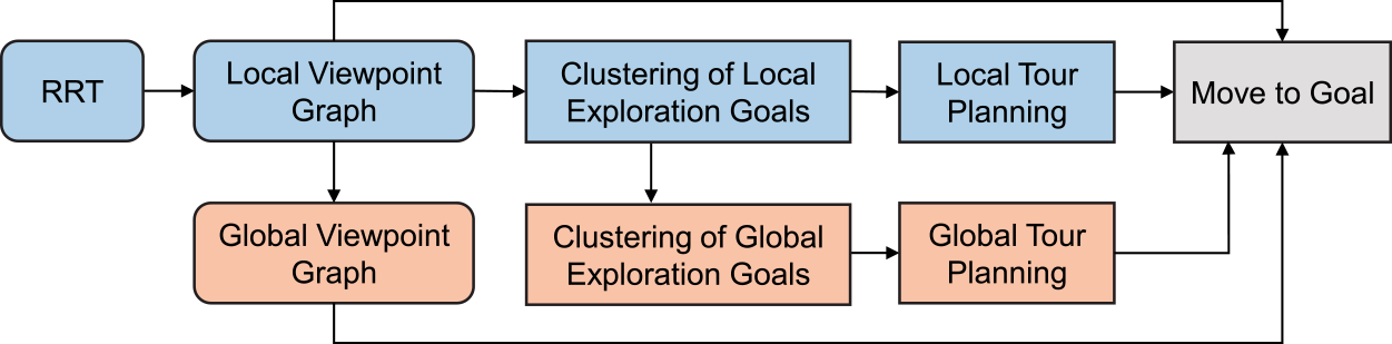
Figure 2. The framework of our exploration method. The blue blocks represent components employed during the exploration stage, whereas the orange blocks denote those utilized in the relocation stage.
Fig. 1 also illustrates the process of detecting local exploration goals. Initially, an RRT is dynamically expanded from the robot position to generate viewpoints within
 $\mathcal{H}$
. Each node on the tree corresponds to a viewpoint, and a local viewpoint graph
$\mathcal{H}$
. Each node on the tree corresponds to a viewpoint, and a local viewpoint graph
 $\mathcal{G}_L$
is constructed using these viewpoints as vertices. The local viewpoint graph helps plan a local navigation path from the current position to a local destination. Subsequently, frontiers are chosen from these viewpoints, defined as
$\mathcal{G}_L$
is constructed using these viewpoints as vertices. The local viewpoint graph helps plan a local navigation path from the current position to a local destination. Subsequently, frontiers are chosen from these viewpoints, defined as
 $\{\mathcal{F}_i\}, i= 1,\cdots,M$
, where
$\{\mathcal{F}_i\}, i= 1,\cdots,M$
, where
 $M$
is the number of frontiers. Specifically, any vertex
$M$
is the number of frontiers. Specifically, any vertex
 $v$
on the graph that meets Equation (2) is regarded as a local frontier. Each local frontier
$v$
on the graph that meets Equation (2) is regarded as a local frontier. Each local frontier
 $\mathcal{F}_i$
is associated with a gain value:
$\mathcal{F}_i$
is associated with a gain value:
 \begin{equation} V(\mathcal{F}_i) = n(u), \forall u \in \mathcal{B}_{\mathcal{F}_i} \wedge u \in \mathcal{S}_{unk} \end{equation}
which is used to select the most promising frontiers for building the global viewpoint graph.
4.1.2. Clustering local exploration goals
The identified local exploration goals
 $\mathcal{F}_L$
are divided into
$\mathcal{F}_L$
are divided into
 $K$
clusters based on their spatial proximity:
$K$
clusters based on their spatial proximity:
 \begin{equation} \mathcal{F}_L = \mathcal{F}_L^1 \cup \cdots \cup \mathcal{F}_L^K, \mathcal{F}_L^i \cap \mathcal{F}_L^j = \emptyset, 1\leq i,j \leq K, i\neq j \end{equation}
Local exploration goals are assigned to the same cluster if their Euclidean distance is less than a tolerance parameter
 $\epsilon$
, specifying the minimum distance between any two clusters:
$\epsilon$
, specifying the minimum distance between any two clusters:
 \begin{equation} \mathcal{F}_L^i \cap \mathcal{F}_L^j = \emptyset \iff d(u,v)\gt \epsilon, \forall u \in \mathcal{F}_L^i, \forall v \in \mathcal{F}_L^j \end{equation}
where
 $d(\cdot,\cdot )$
denotes the Euclidean distance between two spatial points. Note that there is another inherent constraint for spatial clustering. The possible exploration goals are sampled from a local RRT, and the robot can travel freely between any two points without encountering obstacles. This means that, in our context, two clusters positioned on opposite sides of a thin wall can be merged into a single cluster, as long as they originate from the same RRT sampling.
$d(\cdot,\cdot )$
denotes the Euclidean distance between two spatial points. Note that there is another inherent constraint for spatial clustering. The possible exploration goals are sampled from a local RRT, and the robot can travel freely between any two points without encountering obstacles. This means that, in our context, two clusters positioned on opposite sides of a thin wall can be merged into a single cluster, as long as they originate from the same RRT sampling.
For each cluster
 $\mathcal{F}_L^k$
, its centroid is calculated by averaging the 3D positions of all points within the cluster:
$\mathcal{F}_L^k$
, its centroid is calculated by averaging the 3D positions of all points within the cluster:
 \begin{equation} c_{L}^k = \frac{1}{{\left |{\mathcal{F}_L^k} \right |}}\sum \limits _i{{\mathcal{F}_i}}, \mathcal{F}_i \in \mathcal{F}_L^k \end{equation}
where
 $\left |{\mathcal{F}_L^k} \right |$
is the number of local exploration goals in cluster
$\left |{\mathcal{F}_L^k} \right |$
is the number of local exploration goals in cluster
 $\mathcal{F}_L^k$
.
$\mathcal{F}_L^k$
.
As shown in Fig. 3, a navigation goal candidate
 $g_{L}^k$
is selected for each local cluster
$g_{L}^k$
is selected for each local cluster
 $\mathcal{F}_L^k$
. This goal is the furthest point along the direction from the robot position
$\mathcal{F}_L^k$
. This goal is the furthest point along the direction from the robot position
 $P_{rob}$
to
$P_{rob}$
to
 $c_{L}^k$
. In addition, a slight tolerance of direction angle between
$c_{L}^k$
. In addition, a slight tolerance of direction angle between
 $\frac{\vec{g_L^k - c_L^k}}{{\left \|{g_L^k - c_L^k} \right \|}}$
and
$\frac{\vec{g_L^k - c_L^k}}{{\left \|{g_L^k - c_L^k} \right \|}}$
and
 $\frac{\vec{c_L^k -{P_{rob}}}}{{\left \|{c_L^k -{P_{rob}}} \right \|}}$
is allowed. This is done to ensure that the local navigation goal is distant from the current robot position, promoting the coverage of more unknown areas for the next iteration of planning. In the end,
$\frac{\vec{c_L^k -{P_{rob}}}}{{\left \|{c_L^k -{P_{rob}}} \right \|}}$
is allowed. This is done to ensure that the local navigation goal is distant from the current robot position, promoting the coverage of more unknown areas for the next iteration of planning. In the end,
 $K$
local exploration goal clusters will result in
$K$
local exploration goal clusters will result in
 $K$
local navigation goal candidates
$K$
local navigation goal candidates
 $\{g_{L}^k\}, 1\leq k \leq K$
.
$\{g_{L}^k\}, 1\leq k \leq K$
.
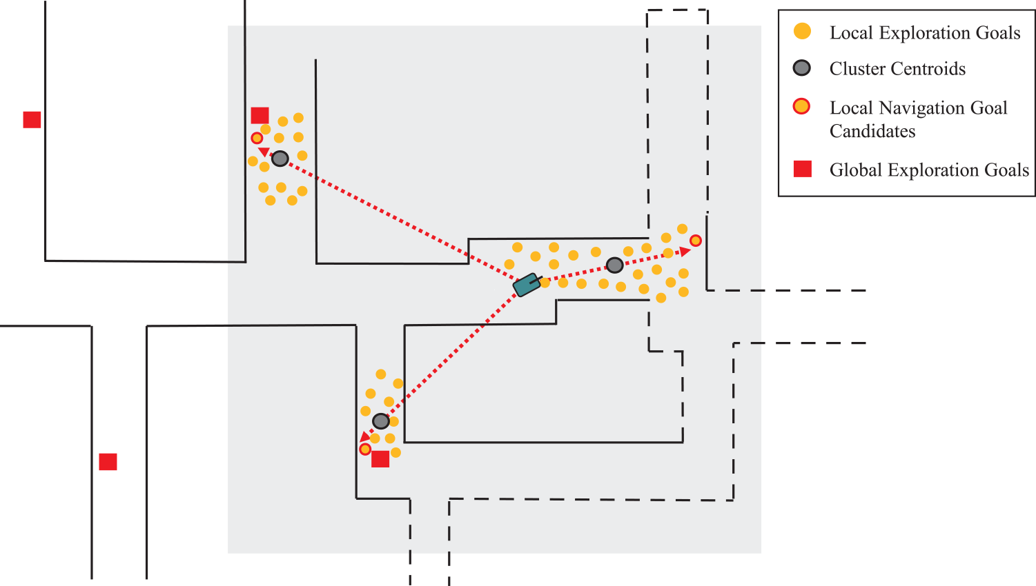
Figure 3. The process of generating local navigation goal candidates. For each exploration goal cluster, the centroid is calculated. The vector from the robot position to the centroid is determined. The furthest point in the vector direction with a slight angle tolerance is selected as the navigation goal candidate.
4.1.3. Local tour planning
The next question is how to determine the best local navigation goal from the candidate set. Inspired by [Reference Zhou, Zhang, Chen and Shen13], we propose solving it as a variant of the TSP. The local navigation goal candidates
 $\{g_{L}^k\}, 1\leq k \leq K$
and the global home position
$\{g_{L}^k\}, 1\leq k \leq K$
and the global home position
 $g_{home}$
serve as places to be visited by a salesman, starting from the current place
$g_{home}$
serve as places to be visited by a salesman, starting from the current place
 $P_{rob}$
. The goal is to compute an optimal open-loop tour that passes through all the local candidate goals and ends at the global home position. Unlike the standard TSP, where the final place to visit is the starting place, here the final place is a specified place (i.e.,
$P_{rob}$
. The goal is to compute an optimal open-loop tour that passes through all the local candidate goals and ends at the global home position. Unlike the standard TSP, where the final place to visit is the starting place, here the final place is a specified place (i.e.,
 $g_{home}$
). We model this as an asymmetric TSP (ATSP) by designing the cost matrix
$g_{home}$
). We model this as an asymmetric TSP (ATSP) by designing the cost matrix
 $C^{ATSP}$
accordingly.
$C^{ATSP}$
accordingly.
 $C^{ATSP}$
is a
$C^{ATSP}$
is a
 $(K+1) \times (K+1)$
square matrix, where the entry
$(K+1) \times (K+1)$
square matrix, where the entry
 $C^{ATSP}_{r,c}$
at row
$C^{ATSP}_{r,c}$
at row
 $r$
and column
$r$
and column
 $c$
denotes the traveling cost from place
$c$
denotes the traveling cost from place
 $r$
to place
$r$
to place
 $c$
. The cost to travel from the current robot position
$c$
. The cost to travel from the current robot position
 $P_{rob}$
to the
$P_{rob}$
to the
 $k$
-th local goal
$k$
-th local goal
 $g_{\mathcal{L}}^k$
is:
$g_{\mathcal{L}}^k$
is:
 \begin{equation} C^{ATSP}_{0,k} = L(P_{rob}, g_{L}^k) + H(P_{rob}, g_{L}^k), k\in \{1,\cdots,K\}, \end{equation}
where
 $L(\cdot,\cdot )$
calculates the shortest path length between two positions according to the local viewpoint graph, and
$L(\cdot,\cdot )$
calculates the shortest path length between two positions according to the local viewpoint graph, and
 $H(\cdot,\cdot )$
calculates the cost of changing the robot heading to the next position. The cost between any two local goals is:
$H(\cdot,\cdot )$
calculates the cost of changing the robot heading to the next position. The cost between any two local goals is:
 \begin{equation} C^{ATSP}_{r,c} = C^{ATSP}_{c,r} = L(g_{L}^r, g_{L}^c), r,c\in \{1,\cdots,K\}. \end{equation}
Considering the first column of
 $C^{ATSP}$
, the item
$C^{ATSP}$
, the item
 $C^{ATSP}_{k,0}$
normally denotes the cost traveling from
$C^{ATSP}_{k,0}$
normally denotes the cost traveling from
 $g_{L}^k$
to
$g_{L}^k$
to
 $P_{rob}$
. We substitute it with the cost traveling from
$P_{rob}$
. We substitute it with the cost traveling from
 $g_{L}^k$
to
$g_{L}^k$
to
 $g_{home}$
:
$g_{home}$
:
 \begin{equation} C^{ATSP}_{k, 0} = L(g_{L}^k, g_{home}), k\in \{1,\cdots,K\}, \end{equation}
where the shortest path length is calculated according to the global viewpoint graph. The advantage of including
 $g_{home}$
in local tour planning will be investigated in Section 5.3. Based on the cost matrix, the ATSP can be solved using existing algorithms. Once the optimal open-loop tour is obtained, the robot proceeds to the first destination on the tour. After reaching the desired goal, the local planning horizon
$g_{home}$
in local tour planning will be investigated in Section 5.3. Based on the cost matrix, the ATSP can be solved using existing algorithms. Once the optimal open-loop tour is obtained, the robot proceeds to the first destination on the tour. After reaching the desired goal, the local planning horizon
 $\mathcal{H}$
is adjusted accordingly, and the exploration stage is repeated until no clusters remain within
$\mathcal{H}$
is adjusted accordingly, and the exploration stage is repeated until no clusters remain within
 $\mathcal{H}$
.
$\mathcal{H}$
.
It’s important to note that the TSP is kept small scale and easy to solve by controlling the number of places in the tour, determined by the size of the local planning horizon and the clustering process. Additionally, the global home position imposes a rigid constraint on the TSP, ensuring the robot returns home regardless of the order in which local goals are visited. However, the global home position is not selected as the next navigation goal during the exploration stage.
4.2. Relocation stage
When there are no remaining exploration goal clusters within
 $\mathcal{H}$
, the robot enters the relocation stage. However, it’s important to note that the algorithm’s parameters may not always suit all types of terrains and environmental structures. Randomly sampling spatial points can sometimes result in an RRT with limited variation or even degeneration. In such cases, the robot may fail to explore certain areas effectively. To enhance the success rate of exploration, we introduce a retrying mechanism before transitioning from exploration to relocation. Specifically, when there are no exploration goal clusters within
$\mathcal{H}$
, the robot enters the relocation stage. However, it’s important to note that the algorithm’s parameters may not always suit all types of terrains and environmental structures. Randomly sampling spatial points can sometimes result in an RRT with limited variation or even degeneration. In such cases, the robot may fail to explore certain areas effectively. To enhance the success rate of exploration, we introduce a retrying mechanism before transitioning from exploration to relocation. Specifically, when there are no exploration goal clusters within
 $\mathcal{H}$
, the RRT is regenerated for further exploration. If the robot still cannot find any exploration goal clusters, it proceeds to the relocation stage. This stage involves clustering global exploration goals, updating the global viewpoint graph, and planning a global tour.
$\mathcal{H}$
, the RRT is regenerated for further exploration. If the robot still cannot find any exploration goal clusters, it proceeds to the relocation stage. This stage involves clustering global exploration goals, updating the global viewpoint graph, and planning a global tour.
4.2.1. Clustering global exploration goals
In each iteration of local tour planning, any remaining local navigation goal candidates that have not been visited before are added to the list of global exploration goals. However, because the information on navigation goals can change during the exploration process, each global exploration goal is double-checked at the beginning of the relocation stage to confirm whether it still represents an unexplored space. This verification can be quickly performed using Equation (1), where the searched space
 $\mathcal{B}_v$
is doubled in
$\mathcal{B}_v$
is doubled in
 $x$
and
$x$
and
 $y$
directions. Any global exploration goals that no longer satisfy Equation (1) are removed from the list. The updated global exploration goals are then denoted as
$y$
directions. Any global exploration goals that no longer satisfy Equation (1) are removed from the list. The updated global exploration goals are then denoted as
 $\{g_G^n\}, 1\leq n \leq N$
.
$\{g_G^n\}, 1\leq n \leq N$
.
In large-scale and convoluted environments, the number of global exploration goals, denoted as
 $N$
, can become excessively large. This will pose a significant challenge for the tour planning process. To address this issue, we propose the utilization of clustering technology to reduce the number of travel destinations when
$N$
, can become excessively large. This will pose a significant challenge for the tour planning process. To address this issue, we propose the utilization of clustering technology to reduce the number of travel destinations when
 $N$
exceeds a predefined threshold, denoted as
$N$
exceeds a predefined threshold, denoted as
 $\rho _{num}$
. Specifically, each global exploration goal is assigned a cost value representing the shortest path length from the global home position to itself. Any two global exploration goals with a cost difference less than
$\rho _{num}$
. Specifically, each global exploration goal is assigned a cost value representing the shortest path length from the global home position to itself. Any two global exploration goals with a cost difference less than
 $\epsilon _{goal}$
are grouped into the same cluster. Within each cluster, we select the exploration goal that is furthest from the home position as a global navigation goal candidate. This approach significantly reduces the number of global navigation goal candidates.
$\epsilon _{goal}$
are grouped into the same cluster. Within each cluster, we select the exploration goal that is furthest from the home position as a global navigation goal candidate. This approach significantly reduces the number of global navigation goal candidates.
4.2.2. Updating global viewpoint graph
The global viewpoint graph plays an important role in computing the travel cost between any two global navigation goal candidates, as well as planning the shortest navigation path from the current robot position to a desired destination within a large-scale space. Following the approach in ref. [Reference Zhu, Cao, Xia, Scherer, Zhang and Wang11], in each iteration of the exploration stage, the local graph vertices on the shortest path from the robot to vertices with positive gain values are added to the global viewpoint graph. The edges are updated accordingly. The global viewpoint graph provides a sparse representation of the environment while still providing short paths between viewpoints.
4.2.3. Global tour planning
During the relocation stage, the primary objective is to find an optimal global tour that guides the robot to visit all global navigation goals and return to the global home position. This is also achieved by implementing an ATSP. The cost matrix, which has a size of
 $(N+1) \times (N+1)$
, is built using Equations (7) – (9) without considering the heading cost. Here, the local candidate goal
$(N+1) \times (N+1)$
, is built using Equations (7) – (9) without considering the heading cost. Here, the local candidate goal
 $\{g_L^k\}, 1\leq k \leq K$
is replaced by
$\{g_L^k\}, 1\leq k \leq K$
is replaced by
 $\{g_G^n\}, 1\leq n \leq N$
.
$\{g_G^n\}, 1\leq n \leq N$
.
Since the number of global navigation goal candidates is suppressed by the clustering step, the global tour planning process can be completed with a satisfactory computational load. The number of iterations required for global tour planning or relocation is also decreased, resulting in significant savings in navigation time. We will investigate the effectiveness of this approach in an ablation study, as discussed in Section 5.3.
4.3. Algorithm implementation
Algorithm 1 provides an overview of the entire exploration process. Throughout this process, a Lidar Odometry and Mapping (LOAM) system plays an important role in estimating the robot’s states and generating the resultant map. Additionally, a terrain traversability analysis module comes into play, generating a terrain map that provides the robot with obstacle information. Based on the terrain map and globally aligned laser scans, two maps,
 $M_{occ}$
and
$M_{occ}$
and
 $M_{octo}$
, are updated at both semantic and metric levels, respectively. Within a defined local planning horizon, an RRT is dynamically expanded based on the information from these semantic and metric maps. The subsequent steps (Lines 7
$M_{octo}$
, are updated at both semantic and metric levels, respectively. Within a defined local planning horizon, an RRT is dynamically expanded based on the information from these semantic and metric maps. The subsequent steps (Lines 7
 $\sim$
17) in the algorithm involve frontier detection, local exploration goal clustering, and local tour planning, as described in Section 4.1. If no local exploration goal clusters are found during the exploration stage, the algorithm allows for one more attempt before transitioning to the relocation stage.
$\sim$
17) in the algorithm involve frontier detection, local exploration goal clustering, and local tour planning, as described in Section 4.1. If no local exploration goal clusters are found during the exploration stage, the algorithm allows for one more attempt before transitioning to the relocation stage.
The following steps implement the relocation stage as described in Section 4.2. Line 23 shows the process of updating global exploration goals, which involves double-checking already existing goals and incorporating newly detected local navigation goals. All global exploration goals are then clustered and employed for tour planning (Lines 25
 $\sim$
30). The strategic application of clustering technology to reduce traveling destinations for tour planning significantly limits computation overhead, especially in large-scale and convoluted environments. Upon successfully navigating the robot to its planned target, it transitions back to the exploration stage. These two stages alternate until no global exploration goals remain. Eventually, the robot returns to its home position, signifying the completion of the exploration task.
$\sim$
30). The strategic application of clustering technology to reduce traveling destinations for tour planning significantly limits computation overhead, especially in large-scale and convoluted environments. Upon successfully navigating the robot to its planned target, it transitions back to the exploration stage. These two stages alternate until no global exploration goals remain. Eventually, the robot returns to its home position, signifying the completion of the exploration task.
Algorithm 1. Exploration in Unknown Environments

5. Experiments
We begin by evaluating the performance of our proposed method in various simulated environments and comparing it with the DSVP method [Reference Zhu, Cao, Xia, Scherer, Zhang and Wang11], which is a challenging autonomous exploration method. Given that DSVP has already been compared with the state-of-the-art methods such as NBVP [Reference Bircher, Kamel, Alexis, Oleynikova and Siegwart19] and GBP [Reference Dang, Tranzatto, Khattak, Mascarich, Alexis and Hutter20], demonstrating its superior performance, we do not replicate those results in this paper. Additionally, we compare our method with the FAEL method [Reference Huang, Zhou, Fan, Zhu, Jie, Li and Cheng21], which also employs tour planning for exploration. Furthermore, we conduct ablation studies to investigate the necessity of specific key operations within our method. Finally, we validate our proposed method through testing on our mobile robot in real-world environments.
5.1. Setup
For the evaluation, we employ a benchmark exploration dataset [Reference Cao, Zhu, Yang, Xia, Choset, Oh and Zhang22] containing five exploration scenarios: indoor, campus, garage, tunnel, and forest. These environments vary in characteristics, with indoor, tunnel, and forest environments featuring narrow passages predominantly, while campus and garage environments offer more spacious areas. These environments are all large-scale and highly convoluted. They are loaded in Gazebo simulator and are unknown to all the methods. All the methods are implemented in the Robot Operating System (ROS) framework. The benchmark exploration platform [Reference Cao, Zhu, Yang, Xia, Choset, Oh and Zhang22] includes a ROS package called “vehicle simulator” to simulate robot kinematics and provide accurate location information. The maximum linear and angular velocities of the simulated robot are set to
 $2 m/s$
and
$2 m/s$
and
 $90 deg/s$
, respectively. Other essential ROS packages for exploration, including collision avoidance, terrain traversability analysis, and path following, are also utilized. DSVP and our planner are launched as independent ROS nodes.
$90 deg/s$
, respectively. Other essential ROS packages for exploration, including collision avoidance, terrain traversability analysis, and path following, are also utilized. DSVP and our planner are launched as independent ROS nodes.
In the implementation, we define
 $\mathcal{B}_v$
as a space of
$\mathcal{B}_v$
as a space of
 $10 \times 10 \times 0.8$
 $m^3$
in Equation (1) and
$m^3$
in Equation (1) and
 $\mathcal{H}$
as a space of
$\mathcal{H}$
as a space of
 $30 \times 30 \times 10$
 $m^3$
in Equation (2).
$m^3$
in Equation (2).
 $\lambda _{num}$
in Equation (1) is set to 10 for narrow environments and 40 for spacious environments. For clustering local exploration goals, we choose
$\lambda _{num}$
in Equation (1) is set to 10 for narrow environments and 40 for spacious environments. For clustering local exploration goals, we choose
 $\epsilon =2 m$
in Equation (5) for narrow environments and
$\epsilon =2 m$
in Equation (5) for narrow environments and
 $\epsilon =3 m$
for spacious environments. Clusters with fewer than
$\epsilon =3 m$
for spacious environments. Clusters with fewer than
 $3$
points are removed. When solving the ATSP for local and global tour planning, a Lin-Kernighan traveling salesman heuristic solver [Reference Helsgaun23] is employed. In Equation (7), the heading cost is defined as
$3$
points are removed. When solving the ATSP for local and global tour planning, a Lin-Kernighan traveling salesman heuristic solver [Reference Helsgaun23] is employed. In Equation (7), the heading cost is defined as
 $\frac{\alpha }{\pi } \cdot 20$
, where
$\frac{\alpha }{\pi } \cdot 20$
, where
 $\alpha$
represents the radians by which the robot should change its heading. If the number of global exploration goals for global tour planning exceeds
$\alpha$
represents the radians by which the robot should change its heading. If the number of global exploration goals for global tour planning exceeds
 $\rho _{num}=40$
, the goals are spatially clustered with a tolerance of
$\rho _{num}=40$
, the goals are spatially clustered with a tolerance of
 $\epsilon _{goal}= 10m$
. Both the DSVP method and our method share default parameters for operations such as RRT generation, graph updates, 3D occupancy mapping, and other relevant activities.
$\epsilon _{goal}= 10m$
. Both the DSVP method and our method share default parameters for operations such as RRT generation, graph updates, 3D occupancy mapping, and other relevant activities.
Each method is run 10 times, with a run ending under the following conditions [Reference Zhu, Cao, Xia, Scherer, Zhang and Wang11]: the exploration algorithm reports completion, the robot moves less than
 $10 m$
within
$10 m$
within
 $300 s$
, or a time limit is reached. We compute the average performance across these 10 runs to compare the methods. All simulations and evaluations are conducted on a Desktop PC equipped with an Intel Core i9-10900KF CPU and 32 GB of memory running Ubuntu 20.04.
$300 s$
, or a time limit is reached. We compute the average performance across these 10 runs to compare the methods. All simulations and evaluations are conducted on a Desktop PC equipped with an Intel Core i9-10900KF CPU and 32 GB of memory running Ubuntu 20.04.
5.2. Results
5.2.1. Area coverage and exploration efficiency
Table I provides an overview of the volumes explored by the compared methods, with the maximum volume across all runs for each environment serving as the ground truth area volume. A run is considered unsuccessful if the explored volume is less than
 $98\%$
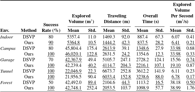
of the ground truth. Table II compares the exploration performances of DSVP and our method. The performance metrics are calculated based on the successful runs.
$98\%$
of the ground truth. Table II compares the exploration performances of DSVP and our method. The performance metrics are calculated based on the successful runs.
Table I. Environment volume estimated by the runs.
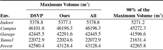
Table II. Comparison of exploration performance.
In the indoor environment, characterized by long and narrow corridors connected with lobby areas, both methods may fail to go through spaces with guard rails, as shown in Fig. 4, due to the randomness of RRT expansion. However, our method demonstrates a slightly higher success rate of 90% compared to DSVP’s 80%. This is attributed to our method’s bias-free RRT expansion, which favors finding sparse local candidate goals that can be reached by the robot. DSVP, on the other hand, biases RRT expansion toward frontiers in large-scale spaces.
Fig. 5 shows the exploration trajectories that are the best of the 10 runs. The best trajectory is from the successful runs and with the highest exploration efficiency. On average, DSVP completes the exploration after traveling 1469.3 m over 887.4 s, while our method takes 837.5 s and travels 1444.2 m. With tour planning, our method facilitates more efficient travel to candidate goals. Despite the need to solve the ATSP, the heuristic solver efficiently handles the limited number of candidate goals in our method. In terms of exploration efficiency, our method covers 6.41
 $m^3/s$
, while DSVP covers 6.07
$m^3/s$
, while DSVP covers 6.07
 $m^3/s$
. Notably, the standard variances of all metrics for our method are lower than those for DSVP, indicating that our method is more efficient and stable.
$m^3/s$
. Notably, the standard variances of all metrics for our method are lower than those for DSVP, indicating that our method is more efficient and stable.
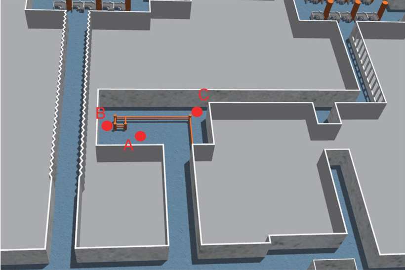
Figure 4. The space with guard rails which occasionally hinders the robot’s passage. During exploration failures, the robot may successfully reach point a but faces difficulties progressing to point C. This is because the laser scans can penetrate the guard rails, resulting in fewer frontiers being detected at point B. If the RRT cannot find a feasible path for extending from point B to point C, the robot will be unable to reach its destination at point C via point B.
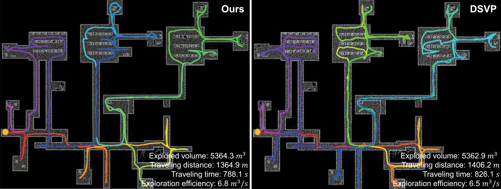
Figure 5. The resulting maps and trajectories of the compared methods for the indoor environment.
In the campus environment with undulating terrains, DSVP achieves a success rate of 80%, while our method achieves 100% by incorporating the retrying mechanism for RRT expansion. However, regenerating the RRT and re-finding local exploration goals add extra time to our method’s process. On average, both methods spend comparable time and travel similar distances to complete the explorations, achieving an exploration efficiency of 33.98
 $m^3/s$
. As shown in Fig. 6, the best trajectory in DSVP outperforms ours. In this environment, where lanes form a star network, tour planning does not significantly impact exploration in our method. Again, our method exhibits lower standard variances across all metrics, indicating greater stability.
$m^3/s$
. As shown in Fig. 6, the best trajectory in DSVP outperforms ours. In this environment, where lanes form a star network, tour planning does not significantly impact exploration in our method. Again, our method exhibits lower standard variances across all metrics, indicating greater stability.

Figure 6. The resulting maps and trajectories of the compared methods for the campus environment.
In the garage environment, featuring multiple floors and sloped terrains, DSVP faces challenges and achieves a success rate of only 70%. In contrast, our method successfully completes the exploration in all runs. On average, our method travels 991 m less distance, takes 512 s less time, and achieves a 3.5
 $m^3/s$
higher exploration efficiency compared to DSVP. Moreover, our method exhibits lower standard variances for explored volume, traveling distance, and overall time, indicating superior efficiency and stability. Qualitative comparisons of the best trajectories, as shown in Fig. 7, support these findings.
$m^3/s$
higher exploration efficiency compared to DSVP. Moreover, our method exhibits lower standard variances for explored volume, traveling distance, and overall time, indicating superior efficiency and stability. Qualitative comparisons of the best trajectories, as shown in Fig. 7, support these findings.
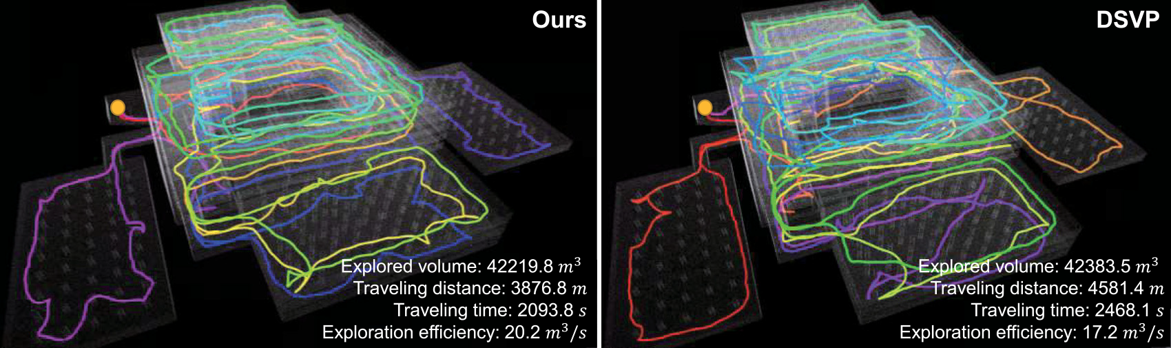
Figure 7. The resulting maps and trajectories of the compared methods for the garage environment.
In the tunnel environment, characterized by a complex network of tunnels, both methods complete the exploration task for all runs. However, our method outperforms DSVP in terms of traveling distance (640 m less), time (374 s less), and exploration efficiency (0.67
 $m^3/s$
higher). Additionally, our method has lower standard variances for most metrics compared to DSVP. Figure 8 shows a qualitative comparison of the best trajectories, demonstrating that our method explores a comparable volume of space with less time and distance.
$m^3/s$
higher). Additionally, our method has lower standard variances for most metrics compared to DSVP. Figure 8 shows a qualitative comparison of the best trajectories, demonstrating that our method explores a comparable volume of space with less time and distance.

Figure 8. The resulting maps and trajectories of the compared methods for the tunnel environment.
In the forest environment with cluttered trees, DSVP tends to explore the space coarsely, resulting in the oversight of many small spaces and a 50% success rate. Our method is able to complete all exploration runs but exhibits slightly higher standard variance. In terms of other metrics, both methods demonstrate comparable performance overall. However, our method achieves a slightly higher exploration efficiency than DSVP, with an additional 0.8
 $m^3/s$
. Qualitative comparisons of the best trajectories for each method, as shown in Fig. 9, further highlight our method’s superior exploration efficiency.
$m^3/s$
. Qualitative comparisons of the best trajectories for each method, as shown in Fig. 9, further highlight our method’s superior exploration efficiency.

Figure 9. The resulting maps and trajectories of the compared methods for the forest environment.
5.2.2. Computational efficiency
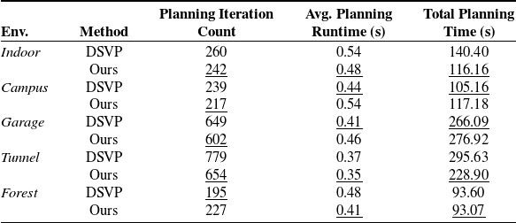
To investigate the computational efficiencies of the methods, the planning iteration count and average planning runtime for each exploration run are recorded. The average values across all runs are presented in Table III. Our method generally requires fewer planning iterations compared to DSVP in most environments. In the indoor, tunnel, and forest environments, our method also exhibits shorter runtimes than DSVP. However, it’s worth noting that in the campus and garage environments, which feature numerous wide spaces, our method generates a larger number of candidate goals, leading to additional time for planning and target selection. Nevertheless, the average planning runtime across all environments remains at approximately 0.45 s, highlighting the efficiency and suitability of our exploration algorithm for real-world mobile robot deployment.
Table III. Comparison of computation efficiencies.
5.2.3. Comparison with other methods
We also execute the open-source FAEL code [Reference Huang, Zhou, Fan, Zhu, Jie, Li and Cheng21] in the same five simulated environments for multiple runs. As shown in Fig. 10, the FAEL method does not prioritize complete area coverage and returning home. It exhibits limitations in fully exploring highly convoluted environments. Sometimes, there may be frequent switches in navigation target selection, particularly within highly convoluted spaces. FAEL appears to be better suited for large unconvoluted spaces, where it balances factors like information gain, movement distance, and coverage efficiency effectively. Since FAEL fails in exploration of the garage environment, characterized by multiple floor and sloped terrains, its compatibility with multi-floor environments remains uncertain.
5.3. Ablation studies
5.3.1. Local tour planning without considering global home position
As indicated in Equation (9), the cost of traveling from any local candidate goal to the current robot position is defined as the distance from the candidate goal to the global home position. We investigate the scenario where the global home position is not taken into account, specifically by setting
 $C^{ATSP}_{k, 0}$
to 0. The revised version of our method is referred to as “Ours_R1.” We perform 10 exploration runs in the indoor environment. The average performance results are presented in Table IV. It shows that, when the global home position is not considered, the method yields comparable exploration coverage and traveling distance but requires more exploration time. Consequently, the exploration efficiency is lower compared to the method that takes the home position into account.
$C^{ATSP}_{k, 0}$
to 0. The revised version of our method is referred to as “Ours_R1.” We perform 10 exploration runs in the indoor environment. The average performance results are presented in Table IV. It shows that, when the global home position is not considered, the method yields comparable exploration coverage and traveling distance but requires more exploration time. Consequently, the exploration efficiency is lower compared to the method that takes the home position into account.
Table IV. Comparison of exploration performance whether considering global home position or not in local tour planning.
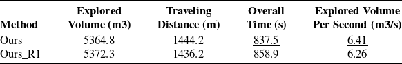

Figure 10. Exploration result of the indoor environment. The white lines denote the trajectories of the robot. It shows that the FAEL method exhibits limitations in fully exploring the highly convoluted environment.
5.3.2. Global tour planning without clustering global exploration goals
In the global tour planning process, the traveling destinations are selected from the global exploration goals for the ATSP. In the experiment, if the number of global exploration goals exceeds 40, they are clustered, resulting in a significant decrease in the number of traveling destinations. Figure 11 (a) shows the change in the number of selected traveling destinations throughout each iteration of global tour planning, when executing exploration in the garage environment. Solving the ATSP with 40 nodes takes about 11 milliseconds. Figure 11 (b) shows the results when clustering is not utilized, during another exploration in the same environment. The maximum number of traveling destinations reaches 114, requiring 48 milliseconds to solve the ATSP. As the number of global exploration goals increases, more iterations of tour planning or relocation are required. Consequently, this leads to an extended overall exploration time.

Figure 11. The number of traveling destinations in global tour planning. When utilizing clustering (a), The number of traveling destinations is significantly reduced, requiring a maximum of 11 milliseconds to solve the ATSP. Without clustering (b), The number of traveling destinations increases significantly, resulting in longer processing times to solve the ATSP and more iterations of tour planning.
5.3.3. Switching to the relocation stage without using retrying mechanism
The effectiveness of employing the retrying mechanism is examined before the robot switches to the relocation stage when no local exploration goals are found. Since the campus and garage environments are characterized by many uneven terrains, they have a more significant influence on the RRT expansion during the exploration stage. We conduct 10 exploration runs in both environments without using the retrying mechanism. The success rates of exploration in the campus and garage environments are 90% and 0%, respectively. The experimental result shows that the RRT has a high possibility of failing to reach unexplored areas when the robot is climbing the ramp between floors. Without attempting to generate the RRT once more, the robot stops exploration and is relocated to a previously recognized space that has not been explored. As shown in Table II, the success rate of exploration reaches 100% in both environments when the retrying mechanism is employed, validating its effectiveness.
5.4. Test in real-world environments
We deploy our exploration package and the benchmark navigation stack [Reference Cao, Zhu, Yang, Xia, Choset, Oh and Zhang22] on our mobile robot platform, which is a four-wheel differential driving mobile robot as shown in Fig. 12. For autonomous exploration, our robot is equipped with a Velodyne VLP-16 lidar and a 6-axis IMU. To handle robot localization and mapping, we utilize a modified version of the LIO-SAM package [Reference Shan, Englot, Meyers, Wang, Ratti and Daniela24], which implements a real-time lidar-inertial odometry. The robot’s maximum linear and angular velocities are set to 0.5 m/s and 15 deg/s, respectively. All packages run on an onboard computer with a 4.8 GHz i7 CPU and 32 GB RAM.

Figure 12. Our mobile robot. For autonomous exploration, it is equipped with a velodyne VLP-16 lidar and a 6-axis IMU. All packages run on an onboard computer with a 4.8 GHz i7 CPU and 32 GB RAM.
The first experiment is conducted on a single floor of a building on our university campus, as shown in Fig. 13. The environment consists of several narrow corridors, intersections, doors, and dead ends. Figure 13 also displays the resulting map and final trajectory obtained by our method. To prevent the robot from entering the bathroom, we placed some static obstacles within the environment. Overall, our method spends 760.2 s traveling a distance of 230.5 m and covering an area of 1928.3 cubic meters. Given the low-speed setting of our mobile platform and the relatively enclosed corridor environment, the exploration efficiency is measured at 2.54
 $m^3/s$
.
$m^3/s$
.

Figure 13. The resulting map and trajectory of our method for a real corridor environment.
In another exploration experiment, we navigate the robot through an underground parking lot of a teaching building on our university campus, as illustrated in Fig. 14. This environment comprises multiple parking spaces with many cars parked, along with building columns and other obstacles. The entry and exit of the parking lot were blocked with static obstacles. The robot begins the exploration near the entry point. After traveling a distance of 567.8 m over a duration of 1243.3 s, the robot successfully completes the exploration. The explored space volume measures 15,077.8 cubic meters, resulting in an exploration efficiency of 12.13
 $m^3/s$
.
$m^3/s$
.

Figure 14. The resulting map and trajectory of our method for a real underground parking lot environment.
These real-world experiments demonstrate the effectiveness of our algorithm when applied to actual mobile robots, highlighting its capacity to efficiently navigate and explore unfamiliar environments.
6. Conclusions
In conclusion, we have presented a dual-stage exploration method that prioritizes simplicity and effectiveness. The spatial clustering and TSP-based tour planning technologies are employed in both stages. In the exploration stage, possible local exploration goals are densely detected from RRT nodes and then spatially clustered. The sparse local navigation goal candidates are extracted from the clusters rather than calculating gains of all possible RRT branches. The local tour planner is further employed to select optimal navigation goals for efficient exploration. In the relocation stage, the number of global exploration goals is also controlled by clustering and the global tour planning effectively guides the robot to revisit unexplored spaces. Our proposed retrying mechanism significantly enhances the success rate of exploration. To evaluate our approach, we conduct tests in five benchmark simulation environments and two real-world environments. Both the simulation and real-world tests demonstrate the effectiveness and efficiency of our method.
However, both DSVP and our methods have certain limitations. Firstly, the system heavily relies on mapping performance and the accuracy of robot localization. It may not perform as expected in open spaces, such as the outdoor areas on campus. Relying solely on laser scans may prove insufficient for detecting obstacles like road curbs or green belts that could pose a danger to the robot. To enhance terrain traversability analysis, integrating additional sensors, such as cameras, would be highly beneficial. Secondly, during the exploration stage, the local graph is utilized to plan the path from the current position to the target goal. Due to the sparse sampling of nodes in the local graph, the planned path may not always be optimal. Furthermore, the planned path is not smoothed in accordance with the robot’s kinematics model. This can result in the robot making frequent heading adjustments, leading to increased power consumption, longer travel times, and posing additional challenges to the simultaneous localization and mapping process. Future work will be dedicated to addressing these identified shortcomings.
Author contributions
Jiatong Bao and Sultan Mamun designed and implemented the exploration method, verified its effectiveness, and wrote the paper. Jiawei Bao set up the simulated and real experimental environments. Wenbing Zhang and Yuequan Yang did the experimental analysis. Aiguo Song guided the progress and reviewed the paper.
Financial support
This research work is supported by the National Natural Science Foundation of China (Grant No. 61806175, 62073322).
Competing interests
The authors declare no competing interests exist.
Ethical standards
Not applicable under the heading.


