


1. Introduction
Motile microorganisms often have to swim through confined geometries in their natural habitats, ranging from navigation of spermatozoa in the female oviduct (Elgeti, Winkler & Gompper Reference Elgeti, Winkler and Gompper2015), movement of pathogens in lung mucus (Huffnagle, Dickson & Lukacs Reference Huffnagle, Dickson and Lukacs2017) and deposition of infectious bacteria in the gastrointestinal tract, to phytoplankton in marine ecosystems (Barry et al. Reference Barry, Rusconi, Guasto and Stocker2015). On the other hand, progress in microfluidic technology has led to the development of lab-on-a-chip devices to characterize in-flow microorganism dynamics to prevent urinary tract infection (Zhou et al. Reference Zhou, Wan, Huang, Li, Peng, Anandkumar, Brady, Sternberg and Daraio2024) or improve clinically assisted reproduction (Huang et al. Reference Huang, Chen, Li and Zhao2023). Furthermore, the artificial counterparts of microorganisms, termed micromotors and nanomotors, are being developed with an aim to achieve targeted drug delivery to infected sites by navigating through complex microcirculation networks (Baraban et al. Reference Baraban, Harazim, Sanchez and Schmidt2013; de Ávila et al. Reference de Ávila2017). Thus an understanding of their propulsive forces and interaction with restricted geometries is inevitable to ensure effective and precise manipulation within the confined pathways.
Interaction of microswimmers with physical boundaries significantly modifies their swimming attributes (Lauga et al. Reference Lauga, DiLuzio, Whitesides and Stone2006; Berke et al. Reference Berke, Turner, Berg and Lauga2008; Di Leonardo et al. Reference Di Leonardo, Dell'Arciprete, Angelani and Iebba2011; Molaei et al. Reference Molaei, Barry, Stocker and Sheng2014; Poddar, Bandopadhyay & Chakraborty Reference Poddar, Bandopadhyay and Chakraborty2021; Damor, Ghosh & Poddar Reference Damor, Ghosh and Poddar2023). The study of Berke et al. (Reference Berke, Turner, Berg and Lauga2008) found that the bacterium Escherichia coli has a tendency to accumulate near the closest surface mainly due to the hydrodynamic forces that cause a wall-parallel reorientation to the swimming bodies. Hydrodynamic interactions with the boundary also lead to circular trajectories of swimming cells near a solid boundary, thereby explaining the mechanism of surface attachment responsible for biofouling and infection (Lauga et al. Reference Lauga, DiLuzio, Whitesides and Stone2006). Similarly, the motility of sperm cells gets affected by the nearby boundary, as revealed in laboratory experiments (Cosson, Huitorel & Gagnon Reference Cosson, Huitorel and Gagnon2003). The surface entrapment of sperm cells poses a challenge to successful insemination in assisted reproductive technologies. Different micro- and nano-structured devices have been proposed (Guidobaldi et al. Reference Guidobaldi, Jeyaram, Condat, Oviedo, Berdakin, Moshchalkov, Giojalas, Silhanek and Marconi2015; Nath et al. Reference Nath, Caprini, Maggi, Zizzari, Arima, Viola, Di Leonardo and Puglisi2023) to prevent surface accumulation. Simultaneous theoretical models were developed to gain insight into the steady height and orientation of microswimmers near the wall during locomotion (Spagnolie & Lauga Reference Spagnolie and Lauga2012; Ishimoto & Gaffney Reference Ishimoto and Gaffney2013; Li & Ardekani Reference Li and Ardekani2014), thereby validating the experimentally observed surface accumulation. Apart from hydrodynamic interaction with the surface, the motility of microorganisms is dependent on several other effects, such as direct flagellar contact (Kantsler et al. Reference Kantsler, Dunkel, Polin and Goldstein2013), pairwise interaction (Drescher et al. Reference Drescher, Dunkel, Cisneros, Ganguly and Goldstein2011), thermal and intrinsic noise (Li & Tang Reference Li and Tang2009; Schaar, Zöttl & Stark Reference Schaar, Zöttl and Stark2015), complex rheology of the surrounding medium (Poddar, Bandopadhyay & Chakraborty Reference Poddar, Bandopadhyay and Chakraborty2019a), and short-range repulsive force (Walker et al. Reference Walker, Wheeler, Ishimoto and Gaffney2019).
The existing background flow modulates self-propulsion in quiescent environments, resulting in fascinating motion behaviours, e.g. navigating against the flow direction (Kaya & Koser Reference Kaya and Koser2012), cross-stream migration (Katuri et al. Reference Katuri, Uspal, Simmchen, Miguel-López and Sánchez2018), jumping or rolling (Sharan et al. Reference Sharan, Xiao, Mancuso, Uspal and Simmchen2022), and trapping in high-shear zones in a microchannel (Rusconi, Guasto & Stocker Reference Rusconi, Guasto and Stocker2014). The change in orientation in response to velocity gradients gives rise to upstream navigation, widely known as ‘rheotaxis’ in relation to a variety of microswimmers, ranging from spermatozoa (Bretherton & Rothschild Reference Bretherton and Rothschild1961; Kantsler et al. Reference Kantsler, Dunkel, Blayney and Goldstein2014) and bacteria (Hill et al. Reference Hill, Kalkanci, McMurry and Koser2007) to artificial microswimmers (Palacci et al. Reference Palacci, Sacanna, Abramian, Barral, Hanson, Grosberg, Pine and Chaikin2015; Baker et al. Reference Baker2019). Rheotaxis has different origins. For sperm in the neighbourhood of liquid–solid interfaces, it is governed by differential drag forces on the head and tail (Rothschild 1963). Combining microfluidic experiments and a mathematical model, Marcos et al. (Reference Marcos, Fu, Powers and Stocker2012) showed that rheotaxis can occur for Bacillus subtilis owing to a critical interaction between the shape asymmetry of the flagella and the velocity gradients in the unbounded domain. Uspal et al. (Reference Uspal, Popescu, Dietrich and Tasinkevych2015) showed the possibility of rheotaxis near a single wall even in the absence of fore–aft asymmetry of the swimmer, e.g. spherical squirmers or Janus particles. The mechanism of shear-induced rotation constrains the upstream motion in the plane of shear. In subsequent investigations, the variations of similar rheotaxis phenomena were analysed for two-dimensional squirmers (Ishimoto Reference Ishimoto2017) and cylindrical-shaped micromotors (Brosseau et al. Reference Brosseau, Usabiaga, Lushi, Wu, Ristroph, Zhang, Ward and Shelley2019), and in the presence of a repulsive wall interaction force (Walker et al. Reference Walker, Wheeler, Ishimoto and Gaffney2019). Similarly, modulations in the background flow can also take place due to an applied electric (Poddar et al. Reference Poddar, Mandal, Bandopadhyay and Chakraborty2018, Reference Poddar, Mandal, Bandopadhyay and Chakraborty2019b), thermal (Mantripragada & Poddar Reference Mantripragada and Poddar2022; Poddar Reference Poddar2023), chemical or magnetic (Tottori & Nelson Reference Tottori and Nelson2018) field.
The motion of microswimmers in confined vessels or channel-like environments brings a new dimension to the motion attributes compared to a single wall. The hydrodynamic interaction with the top and bottom walls leads to unique trajectories such as ‘swinging’ and ‘tumbling’ (Zöttl & Stark Reference Zöttl and Stark2012). During their motion in channels, the existing pressure-driven flows in these passages compete with self-propulsion behaviour (Hill et al. Reference Hill, Kalkanci, McMurry and Koser2007; Jana, Um & Jung Reference Jana, Um and Jung2012; Kaya & Koser Reference Kaya and Koser2012; Mathijssen, Pushkin & Yeomans Reference Mathijssen, Pushkin and Yeomans2015). In experiments, Paramecium describe helical trajectories in glass capillaries (Jana et al. Reference Jana, Um and Jung2012). Jana et al. (Reference Jana, Um and Jung2012) also found that the travelling speed of the organism decreases with tighter confinements due to increased viscous resistance. Similarly, Chlamydomonas sp. cells migrate about the channel axis (Barry et al. Reference Barry, Rusconi, Guasto and Stocker2015). Theoretical studies (Zöttl & Stark Reference Zöttl and Stark2012; Zhu, Lauga & Brandt Reference Zhu, Lauga and Brandt2013) provided further insights by categorizing the swimming states for puller- and pusher-type microswimmers. They reported that puller microswimmers show stable locomotion at the channel centreline, while pushers end up crashing against the walls due to unstable swimming behaviour. It was also reported that swimmers with sufficiently strong dipole strength tend to reach stable states near the walls. In addition, the fluid inertia (Choudhary et al. Reference Choudhary, Paul, Rühle and Stark2022) and complex fluid rheology of microbiological flows (Mathijssen et al. Reference Mathijssen, Doostmohammadi, Yeomans and Shendruk2016) strongly influence the swimming dynamics inside a channel. Recent experiments on microalgae Chlamydomonas (Omori et al. Reference Omori, Kikuchi, Schmitz, Pavlovic, Chuang and Ishikawa2022) demonstrated the existence of rheotaxis and migration to the channel centreline in the presence of cyclic variations of the body deformation and swimming velocity. Along similar lines, oscillatory rheotaxis of self-propelling droplets in microchannels has been reported (Dey et al. Reference Dey, Buness, Hokmabad, Jin and Maass2022).
Surface properties of the geometric confinements have far-reaching consequences on microswimming behaviour. The experiments of Di Leonardo et al. (Reference Di Leonardo, Dell'Arciprete, Angelani and Iebba2011) and Lemelle et al. (Reference Lemelle, Palierne, Chatre, Vaillant and Place2013) revealed that the circular swimming trajectories of E. coli bacteria change sense of rotation near a liquid–solid interface, categorized as an infinite or perfect slip interface. The numerical simulations of Pimponi et al. (Reference Pimponi, Chinappi, Gualtieri and Casciola2016) further predicted that no stable orbit exists for flagellated microswimmers near a similar interface. Surfaces with extreme wettability conditions have been created in various experimental scenarios, such as coating of hydrophobic molecules on surfaces handling a bacterial polymeric solution (Tretheway & Meinhart Reference Tretheway and Meinhart2004; Lauga, Brenner & Stone Reference Lauga, Brenner and Stone2005) or air bubble entrapment in micro- and nano-structured surfaces (Choi & Kim Reference Choi and Kim2006; Lima & Mano Reference Lima and Mano2015). The Navier slip model (Navier Reference Navier1823) had been widely used to model such partial-slip boundaries in different contexts of microfluidics (Chakraborty Reference Chakraborty2008; Vega-Sánchez & Neto Reference Vega-Sánchez and Neto2022). The superhydrophobic boundaries, having high slip lengths, reduce the interfacial friction and fundamentally alter the hydrodynamics. In natural microcirculatory networks, the Navier slip condition can mimic the role of the mucus layer that reduces the interfacial friction (Wang et al. Reference Wang, Ryu, He, Qin and Sung2020). The studies related to microswimmer dynamics near partial-slip boundaries have been limited to either pure self-propulsion (Lopez & Lauga Reference Lopez and Lauga2014; Hu et al. Reference Hu, Wysocki, Winkler and Gompper2015; Poddar, Bandopadhyay & Chakraborty Reference Poddar, Bandopadhyay and Chakraborty2020) or linear shear flow near a wall (Ghosh & Poddar Reference Ghosh and Poddar2023). The mesoscopic simulations of Hu et al. (Reference Hu, Wysocki, Winkler and Gompper2015) suggested the potential of slip-patterned surfaces to convert circular bacterial motion to snaking trajectories. Moreover, contrary to free-slip interfaces, the partial-slip boundaries can produce stable swimming states only when the slip length crosses a critical strength (Poddar et al. Reference Poddar, Bandopadhyay and Chakraborty2020). Under a linear shear flow, the surface hydrophobicity creates a host of new rheotactic states (Ghosh & Poddar Reference Ghosh and Poddar2023) adjacent to the wall, indicating an enhancement in surface entrapment with wall slippage.
It is clear from the above discussion that no attention has been directed in the literature to answer how slip-induced alterations in the flow field around a microswimmer would interact with a background Poiseuille flow due to an applied pressure gradient in a microchannel. Poiseuille flow comes with the additional effects of a quadratic shear flow, which leads to a flow curvature due to the linearly increasing flow gradient. Depending on the unique self-propulsion mechanisms of front or rear actuation (for puller and pusher, respectively), a microswimmer may respond deferentially to the flow gradient in the presence of channel hydrophobicity, or it may need to overcome the drag induced by the flow. Again, the implications of two hydrodynamically interacting planar walls in a slit channel might give rise to non-trivial effects of slip length against the escaping trajectories observed in our earlier works (Poddar et al. Reference Poddar, Bandopadhyay and Chakraborty2020; Ghosh & Poddar Reference Ghosh and Poddar2023).
To address the above unresolved issues in the literature, we present a theoretical model of microswimmer locomotion under the simultaneous influences of Poiseuille flow and hydrodynamic slippage at the confining substrates. We obtain an exact solution of the Stokes flow for a sphere–wall geometry, and apply the superposition method to estimate the effects of both the confining boundaries simultaneously. We employ the Navier slip model (Navier Reference Navier1823) to characterize the substrate wettability. In many earlier studies related to microswimmers in Poiseuille flow, researchers have focused on the force-dipole swimmer models (Mathijssen et al. Reference Mathijssen, Doostmohammadi, Yeomans and Shendruk2016; Choudhary et al. Reference Choudhary, Paul, Rühle and Stark2022; Choudhary & Stark Reference Choudhary and Stark2022), which illustrate the microswimmer as a point particle, thereby neglecting the effects of finite swimmer size (Spagnolie & Lauga Reference Spagnolie and Lauga2012). To resolve this, we provide a semi-analytical solution to the mentioned problem in a bispherical coordinate system, which is competent in capturing the hydrodynamics of a spherical squirmer confined between parallel walls. Furthermore, the force dipole and an image system consisting of point force singularities can predict only the far-field dynamics. In contrast, the present methodology efficiently explains the near-field swimming attributes. Notably, a superposition of the background flow and the flow around a point-like microswimmer can provide important insights into the dynamics when the walls are no-slip in nature (Zöttl & Stark Reference Zöttl and Stark2012). However, a mere inclusion of the Navier slip boundary condition in the background Poiseuille flow, without considering the hydrodynamic interaction with the channel walls, does not accurately represent the impact of slip length on the swimmer's dynamics. This is because the swimming velocity components that affect the dynamics remain unaltered with the slip effect in the absence of hydrodynamic interaction. The presently adopted spherical squirmer model accurately models the slip effects on the active swimming as well as the passive propulsion by incorporating the hydrodynamic interaction, thus rendering the outcome of the study far from intuitive. We further perform a detailed analysis of the dynamic system illustrating microswimmer motion, and categorize the different swimming behaviours.
Analysis of the dynamical system in the plane of background flow reveals the emergence of subcritical Hopf bifurcation with increasing slip lengths for puller microswimmers. On the contrary, the unstable oscillations for pusher microswimmers either transition to damped oscillations or reach a fixed-amplitude oscillatory state. The interaction between a puller and a slippery surface is known to engender new surface rheotaxis states in linear shear flow (Ghosh & Poddar Reference Ghosh and Poddar2023). However, this impact does not create a new stable state at the channel centreline in Poiseuille flow; instead, it causes instability. In this case, it is the pushers that experience the emergence of new stable oscillatory states at the channel centreline due to the slip effect. Also, increasing slip length causes an enhanced tendency to swim downstream in a Poiseuille flow for the same pressure gradient of the imposed flow.
2. Problem formulation
Figure 1 illustrates the physical system under consideration. It displays a spherical microswimmer of radius  $a$ in a slit channel. The large width of a slit channel in the
  $y$ direction lets us consider it as a confined passage between two parallel plates separated by a distance
  $\tilde {H}$ in the
  $z$ direction. Here, the symbol
  $\tilde{\ }$ is used to denote dimensional quantities. The microswimmer is simultaneously actuated by its intrinsic swimming action and a background plane Poiseuille flow, which develops due to an imposed pressure gradient in the channel. The confining boundaries obey the Navier slip boundary condition, quantified by the slip length
  $\tilde {l}_s$. Here, the slip length (
 $\tilde {l}_s$) defines the imaginary distance below (bottom wall) and above (top wall) the bounding walls where the projected flow velocity vanishes. The mathematical form of the Poiseuille flow in the presence of wall slip takes the form
 \begin{equation} \tilde{\boldsymbol{u}}^{(ex)} ={-}\frac{1}{2\mu}\,\frac{{\rm d}\tilde{p}}{{\rm d}\tilde{x}}\,( (\tilde{z}+\tilde{l}_s)\tilde{H} - \tilde{z}^2 ) \boldsymbol{e}_x, \end{equation}
where  $\mu$ is the fluid viscosity, and
  ${\rm d}\tilde {p}/{\rm d}\tilde {x}$ is the applied pressure gradient in the longitudinal direction. The quadratic component in the Poiseuille flow (2.1) gives it a unique feature of non-vanishing shear stress gradient in comparison to a pure linear shear flow. In three dimensions, the orientation of the microswimmer is represented by the director vector
  $\hat {\boldsymbol {p}}$, whose orientation can be described by the angles
  $\theta _p$ and
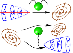
  $\phi _p$, as defined in figure 1. In puller microswimmers, e.g. bacterium Chlamydomonas, the forward movement is achieved by a pulling motion generated by the swimming apparatus located in the front part of the cell body, similar to a breaststroke action. For pusher microswimmers, e.g. sperm cells, the propulsion comes from a pushing motion generated by the posterior (rear) flagellar action. Without any background flow, the flow fields around the microswimmer are shown in the inset using red arrows, while the local forcing directions are marked with blue arrows.

Figure 1. Schematics of a spherical microswimmer confined between two parallel slippery walls separated by distance  $\tilde {H}$ in a background Poiseuille flow taking place in the
  $x$–
$x$– $z$ plane. The centre (
 $O$) of the sphere is located at height
  $\tilde {h}$ from the bottom wall, and the orientation vector is denoted
  $\hat {\boldsymbol {p}}$. The projection of
  $\hat {\boldsymbol {p}}$ on the plane of flow
  $(\hat {\boldsymbol {p}}_{xz})$ is inclined at an angle
  $\theta _p$ with respect to the
  $x$ axis. Similarly, the projection of
  $\hat {\boldsymbol {p}}$ on the
  $x$–
$x$– $y$ plane, i.e.
  $\hat {\boldsymbol {p}}_{xy}$, makes an angle
  $\phi _p$ with the
  $x$ axis. The inset portrays the swimming mechanisms of puller- and pusher-type microswimmers.
We adopt the squirmer model (Lighthill Reference Lighthill1952; Blake Reference Blake1971) to describe the self-propelling mechanism of a spherical microswimmer. In this model, stimulation generated by the appendages of natural microswimmers is captured by small axisymmetric surface distortions on the sphere surface. These distortions are modelled by applying a tangential surface velocity ( $\tilde {\boldsymbol {v}}^{(sp)}_s$) on the microswimmer surface:
 \begin{equation} \tilde{\boldsymbol{v}}^{(sp)}_s=\left(\frac{\hat{\boldsymbol{p}}\boldsymbol{\cdot} \boldsymbol{r}_{s}}{|\boldsymbol{r}_{s}|}\,\frac{\boldsymbol{r}_{s}}{|\boldsymbol{r}_{s}|}-\hat{\boldsymbol{p}}\right) \sum_{n=1}^{\infty} \frac{2}{n(n+1)}\,B_n P'_n\left(\frac{\hat{\boldsymbol{p}}\boldsymbol{\cdot} \boldsymbol{r}_{s} }{|\boldsymbol{r}_{s}|}\right), \end{equation}
where  $B_n$ is the amplitude of the
  $n$th squirming mode,
  $P'_n$ refers to the derivative of the Legendre polynomial with respect to
  $\hat {\boldsymbol {p}}\boldsymbol {\cdot } \boldsymbol {r}_{s}/|\boldsymbol {r}_{s}|$, and
  $\boldsymbol {r}_{s}$ denotes the position vector from the centre of the microswimmer to its surface. Following the previous literature (Uspal et al. Reference Uspal, Popescu, Dietrich and Tasinkevych2015; Shaik & Ardekani Reference Shaik and Ardekani2017), we truncate the infinite series in (2.2) up to the first two squirming modes to capture the essential physics of microswimming. The ratio between the second and first squirmer modes is defined as the squirmer parameter
  $\beta ={B_2}/{B_1}$, which categorizes the squirmers into pullers (
 $\beta >0$), pushers (
 $\beta <0$) and neutral microswimmers (
 $\beta = 0$).
In the following subsections, we develop a mathematical model to identify unique propulsive features due to the interaction between the microswimmer and the Poiseuille flow bounded by slippery confinements.
2.1. Governing equations and boundary conditions
For microorganisms having typical swimming velocity  $\tilde {U}_{ref}$ ranging from tens to hundreds of
  $\mathrm {\mu } \mathrm {m}\ \mathrm {s}^{-1}$, and characteristic length
  $a$ up to a few hundred
  $\mathrm {\mu } \mathrm {m}$, the Reynolds number, defined as
  $Re=\rho \tilde {U}_{ref} a/\mu$, remains mostly of the order of
  $10^{-1}$ or even less (Lauga & Powers Reference Lauga and Powers2009). Thus we can neglect the inertial effects of the flow. It can also be shown that a similar size of microorganisms leads to a very small Péclet number,
  $Pe = \tilde {U}_{ref} a/D$, where
  $D$ is the diffusion coefficient (Stark Reference Stark2016). Accordingly, we neglect the Brownian dynamics (Ishikawa, Simmonds & Pedley Reference Ishikawa, Simmonds and Pedley2006). In order to describe the locomotion of microswimmers in the creeping flow regime, we consider the Stokes equation (Lauga & Powers Reference Lauga and Powers2009). Further considerations of incompressible flow and a Newtonian fluid of viscosity
  $\mu$ reduce the governing equations to
 \begin{equation} \boldsymbol{\nabla} \boldsymbol{\cdot} \tilde{\boldsymbol{v}}=0 \quad \text{and} \quad {-\boldsymbol{\nabla}}\tilde{p}+ \mu\,\nabla ^2 \tilde{\boldsymbol{v}}=0. \end{equation}
Considering the linearity property of the Stokes flow and boundary conditions, we can address the physics of self-propulsion due to squirming action (sp) and external Poiseuille flow (ex) as two separate Stokes flow contributions. Subsequently, the two effects are combined using the relation
 \begin{equation} \gamma=\gamma^{(sp)}+\gamma^{(ex)}, \end{equation}
where  $\gamma$ represents velocity components attained by the microswimmer dictated by different flow triggering mechanisms, i.e.
  $\gamma \in \{\tilde {\boldsymbol {v}}, \tilde {\boldsymbol {V}}, \tilde {\boldsymbol {\varOmega }}\}$.
We non-dimensionalize time by  $a/\tilde {U}_{ref}$ and pressure by
  $\mu \tilde {U}_{ref}/a$. Here, we have considered the swimmer radius
  $a$ as the length scale, and the velocity scale is set as
  $\tilde {U}_{ref}=2B_1/3$ for non-dimensionalization. Finally, in a quiescent medium, the boundary condition on the microswimmer surface due to this squirming action becomes (Lee & Leal Reference Lee and Leal1980)
 \begin{equation} \boldsymbol{v}^{(sp)}=\boldsymbol{V}^{(sp)}+\boldsymbol{\varOmega}^{(sp)} \times \boldsymbol{r}_{s} + \boldsymbol{v}^{(sp)}_s, \end{equation}
where  $\boldsymbol {V}$ and
  $\boldsymbol {\varOmega }$ are the dimensionless translational and rotational velocities, respectively, and
  $\boldsymbol {v}^{(sp)}_s$ is the tangential squirming velocity.
The ambient flow can be considered to be a combination of linear ( $S$) and quadratic (
 $Q$) shear components, defined as
  $\boldsymbol {v}^{(ex)}_{S,\infty } = \mathcal {V}_f (z+l_s)\boldsymbol {e}_x$ and
  $\boldsymbol {v}^{(ex)}_{Q,\infty }= \mathcal {V}_q z^2 \boldsymbol {e}_x$, respectively. Here,
  $\mathcal {V}_f=\tilde {u}_c/\tilde {U}_{ref}$ and
  $\mathcal {V}_q=-\mathcal {V}_f/H$ are the dimensional coefficients for linear and quadratic components, respectively, and
  $\tilde {u}_c = -({\tilde {H}^2}/{8\mu }) ({{\rm d}\tilde {p}}/{{\rm d}\tilde {x}})$ denotes the centreline velocity in the plane Poiseuille flow in the absence of wall slip. This is the maximum velocity in the Poiseuille flow, and thus serves as a convenient scale for the external flow profile. Due to the presence of this external flow field, the sphere exhibits rigid body motion having its translational (
 $\boldsymbol {V}^{(ex)}$) and rotational (
 $\boldsymbol {\varOmega }^{(ex)}$) velocity components. The existence of the sphere within the flow domain engenders a perturbation velocity field (
 $\boldsymbol {v}^{(ex)}$). Finally, the no-slip condition on the particle surface yields the following boundary condition for the perturbation velocity field (
 $\boldsymbol {v}^{(ex)}$):
 \begin{equation} \boldsymbol{v}^{(ex)}=\boldsymbol{V}^{(ex)}+\boldsymbol{\varOmega}^{(ex)} \times \boldsymbol{r}_{s}- \boldsymbol{v}^{(ex)}_{\infty}. \end{equation}
 The Navier slip boundary condition (Navier Reference Navier1823) at the confinement boundaries relates the tangential components of the surface velocity at the confinement boundaries ( $\tilde {\boldsymbol {v}}_{\|}$) to the local shear rate by the relation
 \begin{equation} \text{at } z= 0, H, \quad \boldsymbol{v}_{\|}= l_s \boldsymbol{n}_w\boldsymbol{\cdot}(\boldsymbol{\nabla} \boldsymbol{v}+(\boldsymbol{\nabla} \boldsymbol{v})^{\rm T})(\mathcal{I}-\boldsymbol{n}_w\boldsymbol{n}_w ), \end{equation}
where  $\mathcal {I}$ is the identity tensor, and
  $\boldsymbol {n}_w$ represents the unit normal to the planar confinements towards the channel axis.
We consider the squirmer to be neutrally buoyant, and disregard any non-hydrodynamic forces that may arise due to surface interactions close to the walls. Hence we can compute the unknown microswimmer velocities  $\boldsymbol {V}$ and
  $\boldsymbol {\varOmega }$, generated due to the combined effect of squirming action and external Poiseuille flow, by employing the following force- and torque-free conditions:
 \begin{equation} \boldsymbol{F}= \iint_{S_p} \boldsymbol{{\sigma}}\boldsymbol{\cdot} \boldsymbol{n_p}\, {\rm d}S=0 \quad \text{and} \quad \boldsymbol{L}= \iint_{S_p} \boldsymbol{r}_{s} \times (\boldsymbol{{\sigma}}\boldsymbol{\cdot} \boldsymbol{n_p})\, {\rm d}S=0, \end{equation}
respectively. The microswimmer attains the thrust force and torque required for its propulsion from both the squirming action ( $\boldsymbol {F}_T^{(sp)}, \boldsymbol {L}_T^{(sp)}$) and the Poiseuille flow (
 $\boldsymbol {F}_T^{(ex)}, \boldsymbol {L}_T^{(ex)}$). These forces and torques are balanced by the hydrodynamic drag force (
 $\boldsymbol {F}_D$) and torque (
 $\boldsymbol {L}_D$) experienced by the microswimmer.
2.2. Solution methodology
We employ a combined analytical–numerical solution strategy for the Stokes flow (2.3) in a single-wall–squirmer configuration. The method is premised on the general solution of the Stokes equation using the eigenfunction expansion in the bispherical coordinate system  $( \xi, \eta, \phi )$ (Lee & Leal Reference Lee and Leal1980; Behera, Poddar & Chakraborty Reference Behera, Poddar and Chakraborty2023; Poddar Reference Poddar2023). Our previous works contain a detailed description of the solution methodology for a single-wall system in the cases where a squirmer is in a linear shear flow (Ghosh & Poddar Reference Ghosh and Poddar2023) and in a quiescent medium (Poddar et al. Reference Poddar, Bandopadhyay and Chakraborty2020). The part of the boundary condition on the particle surface (2.6) that exists for a fixed particle in the ambient flow, i.e.
  $\boldsymbol {v}^{(ex)}(\text {at } r=1)= - \boldsymbol {v}^{(ex)}_{\infty }$, is expressed in terms of the coefficients
  $X^m_n$,
  $Y^m_n$ and
  $Z^m_n$ (Lee & Leal Reference Lee and Leal1980) to obtain the solution of the corresponding Stokes problem in terms of bispherical eigenfunctions. These constants, derived here for the case of a parabolic shear flow, are given as
 \begin{equation} X_n^1=0, \quad Z_n^1=0\\ \end{equation}
and
 \begin{equation} Y_n^1={-}4 \sqrt{2}\sinh(\xi_0)\,(n+\tfrac{1}{2})\,{\rm e}^{-(n+{1}/{2})\xi} [\mathcal{V}_f+\mathcal{V}_q(\sinh(\xi_0)\,(n+\tfrac{1}{2})+\cosh(\xi_0))], \end{equation}
where  $\xi _0$ corresponds to the location of the sphere surface in bispherical coordinates. The corresponding thrust force and torque components on the particle are given by
 \begin{align} F^{(ex)}_{(T,x)}&={-}{\sqrt{2}\,{\rm \pi}} ((l_s+\cosh(\xi_0)\,\mathcal{V}_f+\mathcal{V}_q(\cosh(\xi_0))^2)\sinh(\xi_0)\nonumber\\ &\quad \times \sum_{n=0}^{\infty}[G_n^1-H_n^1+n(n+1)(A_n^1-B_n^1) ], \end{align}
 \begin{align} L^{(ex)}_{(T,y)} &={\sqrt{2}\,{\rm \pi}}(2\mathcal{V}_f + \mathcal{V}_q \cosh(\xi_0))\sinh^2(\xi_0) \nonumber\\ &\quad \times \sum_{n=0}^{\infty} [\coth(\xi_0)\,\{n(n+1)(A_n^1-B_n^1)+(G_n^1-H_n^1)\}\nonumber\\ &\quad -2n(n+1)C_n^1 -(2n+1)(G_n^1-H_n^1) ]. \end{align}
2.2.1. Simultaneous influence of the two boundaries
The bispherical method cannot be applied directly to calculate the hydrodynamic resistance offered by the two interacting parallel walls. To resolve this issue, we adopt the superposition method proposed in the literature (Ho & Leal Reference Ho and Leal1974; Pasol et al. Reference Pasol, Martin, Ekiel-Jeżewska, Wajnryb, Bławzdziewicz and Feuillebois2011; Ghalya et al. Reference Ghalya, Sellier, Ekiel-Jeżewska and Feuillebois2020). It was reported that the superposition of particle velocities obtained from the individual effects of the two walls could precisely capture the particle velocity in the presence of an external flow. The detailed numerical investigations (Jones Reference Jones2004; Pasol et al. Reference Pasol, Martin, Ekiel-Jeżewska, Wajnryb, Bławzdziewicz and Feuillebois2011) brought out that the superposition method is reasonably accurate in the range  $H>4$, i.e. when the channel width is broad relative to the particle radius. Along similar lines, in Appendix A, we compare our superposition method results against the detailed boundary-integral results of Staben, Zinchenko & Davis (Reference Staben, Zinchenko and Davis2003) for the movement of a passive spherical particle placed between two infinite parallel walls in a plane Poiseuille flow. Good agreement between present calculations and the earlier results can be observed in figure 18. On the other hand, a similar superposition approach for two walls has also been used for the force dipole model of microswimmers (Zöttl & Stark Reference Zöttl and Stark2012; Choudhary & Stark Reference Choudhary and Stark2022). In the present method, the effective translational and rotational velocities are calculated by superposing the individual wall effects and subtracting the velocities in the unbounded domain to compensate for the repeated account of the same effect. Thus the velocity components can be obtained as
 \begin{equation} \boldsymbol{V}=\boldsymbol{V}^{(1)}+\boldsymbol{V}^{(2)}-\boldsymbol{V}^{(0)} \quad \text{and}\quad \boldsymbol{\varOmega}=\boldsymbol{\varOmega}^{(1)} - \boldsymbol{\varOmega}^{(2)}-\boldsymbol{\varOmega}^{(0)}, \end{equation}
where  $\boldsymbol {V}^{(1)}$ (
 $\boldsymbol {\varOmega }^{(1)}$) and
  $\boldsymbol {V}^{(2)}$ (
 $\boldsymbol {\varOmega }^{(2)}$) are the translational (rotational) velocities of the microswimmer due to the sole presence of the bottom and top wall, respectively. In addition,
  $\boldsymbol {V}^{(0)}$ and
  $\boldsymbol {\varOmega }^{(0)}$ are the translation and rotation velocities of the microswimmer in Poiseuille flow in the absence of the bounding walls. Even though this approach remains intuitive for a passive particle, the asymmetry of a squirming sphere prohibits results from a single-wall scenario from being extrapolated to a corresponding two-wall situation owing to the different orientations of the director (
 $\hat {\boldsymbol {p}}$) relative to each wall, which is portrayed in figure 2. In figure 2(c), we show how the actual upper-wall–sphere configuration can be replaced by a conceptually equivalent lower-wall–sphere configuration. In the case of a passive particle, it would have been sufficient to consider the complementary distance
  $H-h$ from the top wall. However, in the case of microswimmer, one has to additionally account for the changed orientation of the director relative to the upper wall, i.e.
  $180^{\circ }+\theta _p$ instead of
  $\theta _p$ if the effect of the upper wall has to be calculated just by considering a single wall. Consequently, the velocity components
  $\boldsymbol {V}^{(2)}$ and
  $\boldsymbol {\varOmega }^{(2)}$ of the upper wall have been calculated for the equivalent lower wall instead of the upper wall, as shown in figure 2(c). This orientational asymmetry about the centreline creates asymmetry in the microswimmer velocity components about the centreline, as shown in figure 3.

Figure 2. Schematics of the microswimmer configuration: (a) in the actual two-wall scenario; (b) relative to the lower wall only; and (c) relative to an equivalent lower wall for the upper wall.

Figure 3. Variation of  $\varOmega _y$ of a puller microswimmer (
 $\beta =3$) for varying gaps from the lower wall (
 $h$) and different slip lengths (
 $l_s$) in the absence of any external flow. The angular orientation is fixed at
  $\theta _p=45^{\circ }$ when measured relative to the lower wall. The inset shows the case
  $\theta _p=225^{\circ }$.
The velocity components of the microswimmer due to the self-propulsion in an unbounded domain are given by
 \begin{equation} {V}_x^{(sp, 0)}= \cos(\theta_p), \quad \varOmega_y^{(sp,0)}= 0 \quad \text{and} \quad V_z^{(sp, 0)}={-}\sin(\theta_p). \end{equation}
The velocity components of a passive particle in a general ambient flow field  $\boldsymbol {v}^{(ex)}_\infty$ in an unbounded domain can be calculated by invoking the Faxén law (Kim & Karrila Reference Kim and Karrila2013):
 \begin{equation} \boldsymbol{V}^{(ex,0)}=\left(\boldsymbol{v}^{(ex)}_\infty+\frac{\nabla^2\boldsymbol{v}^{(ex)}_\infty}{6} \right)_{\text{at }z=h} \quad \text{and} \quad \boldsymbol{\varOmega}^{(ex,0)}= \frac{1}{2}\,(\boldsymbol{\nabla} \times \boldsymbol{v}^{(ex)}_\infty)_{at\ z=h}. \end{equation}
Using the present form of external flow (2.1), we get
 \begin{equation} \boldsymbol{V}^{(ex,0)}=( \mathcal{V}_f (l_s+h) + \mathcal{V}_q (h^2+\tfrac{1}{3}) ) \boldsymbol{e}_x \quad \text{and} \quad \boldsymbol{\varOmega}^{(ex,0)}= \tfrac{1}{2} (\mathcal{V}_f+2\mathcal{V}_qh) \boldsymbol{e}_y. \end{equation}
The term  $\mathcal {V}_q /3$ in the expression for
  $\boldsymbol {V}^{(ex,0)}$ signifies the effect of flow curvature on the particle motion in the unbounded domain.
The mathematical model presented above brings out the following key dimensionless parameters influencing the flow physics: the slip length  $l_s$, squirmer parameter
  $\beta$, channel height relative to the microswimmer radius
  $H$, and external flow strength relative to the intrinsic swimming speed
  $\mathcal {V}_f$.
2.3. Three-dimensional dynamics
The microswimmer axis may deviate from the  $x$–
$x$– $z$ plane due to perturbations in actual experiments. Thus we perform a three-dimensional (3-D) analysis of the microswimmer dynamics to check the validity of the attractor fixed points and attractive limit cycles discovered in the above subsections against perturbation of the microswimmer axis in the vorticity direction.
Without hydrodynamic interaction of the microswimmer with the bounding walls, the two-dimensional phase-space remains similar to the 3-D problem (Zöttl Reference Zöttl2014). However, the inclusion of hydrodynamic interaction in the model non-trivially alters the stability behaviour of near-wall fixed points. As reported in Uspal et al. (Reference Uspal, Popescu, Dietrich and Tasinkevych2015), for an external linear shear flow, some of the near-wall stable attractors may become unstable in three dimensions. To understand whether the slip length has any effect on our results, we calculate the out-of-plane dynamics as follows. Different components of the director vector can be expressed in a general 3-D space as
 \begin{equation} p_x = \cos{\theta_p}\cos{\phi_p}, \quad p_y = \cos{\theta_p}\sin{\phi_p} \quad \text{and} \quad p_z ={-} \sin{\theta_p}. \end{equation}
Thus the quasi-steady dynamics (3.1) can be obtained by solving the following coupled ordinary differential equations (ODEs):
 $$\begin{gather} \frac{{\rm d} x}{{\rm d}t}=\mathcal{V}_f V_x^{(ex)} + V_x^{(sp)} \cos(\phi_p), \quad \frac{{\rm d}\kern0.05em y}{{\rm d}t}= V_x^{(sp)} \sin(\phi_p), \quad \frac{{\rm d}z}{{\rm d}t}= V_z^{(sp)}, \end{gather}$$
 $$\begin{gather}\frac{{\rm d}p_x}{{\rm d}t} = \varOmega_y p_z-\varOmega_z p_y, \quad \frac{{\rm d}p_y}{{\rm d}t} ={-}\varOmega_x p_z+\varOmega_z p_x, \quad \frac{{\rm d}p_z}{{\rm d}t} = \varOmega_x p_y-\varOmega_y p_x, \end{gather}$$
where
 \begin{equation} \varOmega_x ={-} \varOmega_y^{(sp)} \sin(\phi_p), \quad \varOmega_y = \mathcal{V}_f \varOmega_y^{(ex)} + \varOmega_y^{(sp)} \cos(\phi_p) \quad \text{and} \quad \varOmega_z=0. \end{equation}
3. Results and discussion
This section demonstrates the locomotion behaviour of a microswimmer navigating through a confined Poiseuille flow in the presence of slippery walls. The estimation of the dimensionless parameters is based on various practical considerations, as mentioned below. In the microfluidic experiments of Junot et al. (Reference Junot, Figueroa-Morales, Darnige, Lindner, Soto, Auradou and Clément2019), the flow rate of the external pressure driven flow was varied in the range  $Q = 1\unicode{x2013}6$ nl s
 $^{-1}$, giving the maximum external flow velocity as
  $\tilde {u}_c = 28\unicode{x2013}168\ \mathrm {\mu } {\rm m} {\rm s}^{-1}$, whereas the intrinsic bacteria velocity was found to be
  $\tilde {U}_{ref} = 20\unicode{x2013}30\ \mathrm {\mu } {\rm m}\ {\rm s}^{-1}$. On the other hand, the experiments of Dey et al. (Reference Dey, Buness, Hokmabad, Jin and Maass2022) reported an intrinsic swimming speed
  $\tilde {U}_{ref} \approx 30\ \mathrm {\mu } {\rm m}\ {\rm s}^{-1}$ for self-propelling droplets. The external flow rate used by them was comparatively lower, i.e.
  $\tilde {Q} = 0.04\unicode{x2013}0.094 \ \mathrm {nl s}^{-1}$, resulting in a maximum external flow velocity
  $\tilde {u}_c = 11.55\unicode{x2013}27.15 \ \mathrm {\mu } {\rm m}\ {\rm s}^{-1}$. These available studies suggest the practical range of the dimensionless parameter
  $\mathcal {V}_f$ as 0.385–8.4. In view of these reported ranges of
  $\mathcal {V}_f$ and the values used in earlier theoretical studies (Zöttl & Stark Reference Zöttl and Stark2012; Choudhary & Stark Reference Choudhary and Stark2022), we have used
  $\mathcal {V}_f$ in the range 0–25. Unless mentioned otherwise, the results have been demonstrated for
  $H = 6$. We take into account two constraints imposed by the flow physics and the mathematical model for determining the distance
  $H$ between the parallel plates. First, a very narrow channel violating the limit
  $H > 4$ may not provide accurate numerical results due to the breakdown of the superposition method (§ 2.2.1). Second, for a broad channel height, it is sufficient to consider the linear part of the external flow only near a wall (Katuri et al. Reference Katuri, Uspal, Simmchen, Miguel-López and Sánchez2018), thus obscuring the new physics of flow curvature associated with the parabolic shear flow. Further, motivated by the experimental evidence of varied slip lengths for diverse nano-engineered surface properties, such as hydrophobicity (Choi & Kim Reference Choi and Kim2006) and ‘intrinsic slippage’ (Gentili et al. Reference Gentili, Bolognesi, Giacomello, Chinappi and Casciola2014), the results are demonstrated for a wide range of dimensionless slip lengths, i.e.
  $l_s = 0$–10.
The quasi-steady dynamics of the microswimmer can be described by solving the coupled ODEs
 \begin{equation} \frac{{\rm d}\boldsymbol{r}(t)}{{\rm d}t}=\boldsymbol{V} (\boldsymbol{r}(t),\hat{\boldsymbol{p}}(t))\quad \text{and} \quad \frac{{\rm d}\hat{\boldsymbol{p}(t)}}{{\rm d}t}=\boldsymbol{\varOmega}(\boldsymbol{r}(t),\hat{\boldsymbol{p}}(t)) \times \hat{\boldsymbol{p}}(t), \end{equation}
where the initial conditions required to solve these ODEs in the plane of external flow are specified as  $\boldsymbol {r}(t=0) = (0, 0, h_0)$ and
  $\hat {\boldsymbol {p}}(t=0) = (\cos (\theta _{0}), 0, -\sin (\theta _{0}))$, where
  $h_0$ and
  $\theta _{0}$ denote the initial height of the microswimmer centre from the bottom wall and its orientation angle, respectively. We have calculated the microswimmer trajectories by integrating (3.1a,b) using the fourth-order Runge–Kutta scheme (Chapra Reference Chapra2010). Here, we consider only the impacts of deterministic hydrodynamic forces, and ignore the stochastic forces (Shum, Gaffney & Smith Reference Shum, Gaffney and Smith2010; Spagnolie & Lauga Reference Spagnolie and Lauga2012). In addition, to avoid the effect of non-hydrodynamic forces due to surface interactions, we limit the lateral range of the computational domain to
  $1.01 \le h \le H-1.01$. The microswimmer dynamics in the plane of external flow (i.e.
  $x$–
$x$– $z$ plane) can be captured by solving the plane autonomous system
 \begin{equation} \frac{{\rm d}z}{{\rm d}t}= V_z(z,t) \quad \text{and} \quad \frac{{\rm d}\theta_p}{{\rm d}t}= \varOmega_y(z,t). \end{equation}
We make use of the dynamic system theory to understand the microswimmer dynamics. Due to the non-existence of explicit analytical expressions for the eigenvalues of the linearized system at fixed points, we employ a graphical approach to identify the stability criterion and observe instances of bifurcation. To this end, we generate phase portraits for the planar dynamics for a broad range parameters  $l_s$ and
  $\mathcal {V}_f$ chosen at fine intervals. Given the invariance of the dynamic system along
  $x$, we distinguish the motion behaviours in the upstream or downstream directions by computing the long-term trajectories for the critical cases observed in the phase portraits. It is noteworthy that in the absence of slip, combining the background flow and the flow around a point-like microswimmer provides crucial information on the dynamics even without hydrodynamic interaction (Zöttl & Stark Reference Zöttl and Stark2012). However, mere inclusion of the Navier slip boundary condition (2.7) in the background Poiseuille flow, without incorporating the hydrodynamic interaction with the channel walls, cannot track the effect of slip length on the swimmer dynamics. This is because the microswimmer velocity components
  $V_z$ and
  $\varOmega _y$ remain unchanged with
  $l_s$ when no hydrodynamic interaction is considered in the model. The hydrodynamic interaction is influenced by the slip effect, as described in figure 3. The figure shows that adjacent to the confining substrates, the rotational velocity of the microswimmer
  $\varOmega _y$ significantly increases or even changes its sign in comparison to the no-slip scenario. Moreover, the inset with
  $\theta _p=225^{\circ }$ in figure 3 displays a mirror symmetry of
  $\varOmega _y$ variation relative to the
  $\theta _p=45^{\circ }$ case, confirming an expected symmetry for self-propulsion between parallel walls in the absence of any external flow.
3.1. Transition of swimming states for pullers
We analyse the diverse swimming features of the pullers by categorizing the results into two broad ranges of  $\mathcal {V}_f$, i.e. weak background flow (
 $0 \le \mathcal {V}_f \le 1$) and strong background flow (
 $1 < \mathcal {V}_f \le 25$).
3.1.1. Weak background flow regime
The phase portraits for in-plane dynamics and corresponding sample trajectories in this regime are presented in figure 4. To shed light on the diverse physical processes represented by the phase portraits, we illustrate the effects of self-propulsion (‘sp’) and external flow (‘ex’) on various velocity components in figure 5. Moreover, we present regime maps highlighting different swimming states in figure 6 to summarize the impacts of various combinations of the governing factors on microswimming. Finally, the out-of-plane stability of the microswimmer and its long-time dynamics in three dimensions are described in figures 7 and 8.

Figure 4. Phase portraits for in-plane dynamics and corresponding trajectories for a puller microswimmer. Different slip lengths in (a–c) are  $l_s= 0$,
  $1.35$ and
  $5$, respectively, while other parameters are chosen as
  ${\beta =3}$ and
  $\mathcal {V}_f=0.6$. Squirmer parameter
  $\beta =7$ is used in (d)
  $\mathcal {V}_f=0.1$,
  $l_s=0.05$, (e)
  $\mathcal {V}_f=0.4$,
  $l_s=0.05$, and ( f)
  $\mathcal {V}_f=0.4$,
  $l_s=1.35$. The stable and unstable spiral states are indicated with filled and unfilled black stars, respectively, whereas the green crosses indicate the saddle points. The red lines in the phase portraits denote the corresponding selected trajectories in (g,h), with the red dots indicating the initial locations. (g) Different contrasting stable and unstable trajectories corresponding to the phase portraits in (a–c). (h) The contrasting feature of the coexistence of a near-wall stable and a centreline stable state corresponding to the phase portrait in (e). Trajectories at different combinations of
  $l_s$ and
  $\mathcal {V}_f$ are presented for (g)
  $\beta =3$ and (h)
  $\beta =7$.

Figure 5. (a) Contributions of external flow strength and self-propulsion in  $V_x$ for different slip lengths. (b–d) Variations of
  $\varOmega _y$ for
  $l_s= 0$,
  $1.35$ and
  $5$, respectively. Other parameters are
  $\mathcal {V}_f=0.6$ and
  $\beta =3$.

Figure 6. Regime maps for pullers with (a)  $\beta =3$ and (b)
  $\beta =7$, for
  $\mathcal {V}_f < 1$. The different zones in the regime maps are designated as: (I) blue triangular markers for stable oscillation states about the channel centreline; (II) green triangular markers for unstable oscillation states about the channel centreline only; (III) black square markers for coexistence of near-wall (downstream) and centreline (upstream) steady states; (IV) red circular markers for coexistence of near-wall (upstream) and centreline (upstream) steady states; (V) yellow square markers for near-wall steady states (both upstream and downstream) only. In addition, the black cross markers denote the collision of the microswimmer with the walls. The downstream (upstream) oscillations are encoded in the triangular markers by pointing them towards the right (left).

Figure 7. Comparison of trajectories of pullers for a small perturbation of the initial condition from the plane of external flow ( $\phi _0=1^{\circ }$) and those released in the plane of flow (
 $\phi _0=0^{\circ }$). (a) Downstream centreline oscillations of a puller (
 $\beta =3$) at
  $l_s=1.35$ and
  $\mathcal {V}_f=0.6$. (b–d) Highlighting the stability of (b) centreline and (c,d) near-wall trajectories of a puller (
 $\beta =7$) with
  $l_s=0.05$ and
  $\mathcal {V}_f=0.4$. The centreline trajectories are captured at
  $h_0=3$ and
  $\theta _p=165^{\circ }$ in (a) and (b). Near-wall states are plotted for (c)
  $h_0=2$ and (d)
  $h_0=1.3$.

Figure 8. Out-of-plane dynamics of pullers in the weak background flow regime. (a–c) Regime maps for a puller ( $\beta =3$) summarizing the 3-D dynamics at different slip lengths
  $l_s= 0$, 1.35 and 5, and (d–h) corresponding trajectories. (i) Regime map to summarize the near-wall states for
  $\beta =7$ and
  $h_0=1.3$, and (j,k) corresponding sample trajectories. Zones I (green), II (blue), III (red) and IV (yellow) represent centreline stable upstream, centreline stable downstream, collision, and stable near-wall state, respectively.
Phase portraits with a low strength of the squirmer parameter, i.e.  $\beta =3$, are shown in figures 4(a–c). There exists an attractive spiral at the core of the phase space when a puller is confined between no-slip walls in a plane Poiseuille flow (figure 4a). This indicates damped amplitude oscillations of the microswimmer about the channel centreline. Similar motion features have been termed ‘swinging’ in the literature (Zöttl & Stark Reference Zöttl and Stark2012). The corresponding trajectory in figure 4(g) demonstrates that these stable oscillations occur upstream to the flow direction (blue trajectory). At a sufficiently enhanced slip length (
 $l_s=1.35$), the attractive spiral shows a slower decay (figure 4b). In addition, the axial motion switches to the downstream direction, as shown by the green curve in figure 4(g). This outcome carries substantial consequences in pressure-driven flow through a microchannel. They indicate the feasibility of reversing the motion direction of a microswimmer using the same pressure gradient in a slippery channel. This observation can be justified by the effects of hydrodynamic slip on the Poiseuille flow. Slip reduces the viscous friction offered to the flow by the walls. It can be shown that the effective flow rate is consequently increased by the factor
  $Q_{slip}/Q_{no\text {-}slip} = 1+ 6 \, l_s/H$. As a result, the microswimmer experiences a greater force pushing it forwards in the direction of the flow, resulting in a greater tendency to swim in that direction. The effect of slip is not limited to the change in effective bulk flow rate. It has more significant consequences on the flow distribution, resulting in altered hydrodynamic interaction with the boundaries. This is reflected in the disruption of the stability condition at a high slip length, as observed in figure 4(c) for
  $l_s=5$. The black curve in figure 4(g) shows that an unstable oscillation state is created in the downstream direction. Due to increasing amplitudes of oscillations, the swimmer finally crashes against one of the walls. It is to be noted that we have not included any repulsive interaction at the channel walls in order to focus exclusively on the hydrodynamic interaction behaviour (Zöttl & Stark Reference Zöttl and Stark2012; Uspal et al. Reference Uspal, Popescu, Dietrich and Tasinkevych2015). In figure 4(g), we have shown a case where an unstable upstream swimming state has been created at a lower strength of external flow (
 $\mathcal {V}_f=0.2$) and high slip length (
 $l_s=5$). Such differential motion behaviour indicates the competitive effects of slip length and flow strength on microswimmer locomotion.
The capacity of slip length to alter the swimming state along the centreline underlines the fact that slip effects on the dynamics are not restricted to the near-wall zones only, although the slip-induced perturbation for a fixed orientation of the swimmer vanishes at the centreline (figure 3). This apparent anomaly can be explained by the change in the near-wall velocities that alter the instantaneous configuration  $(h,\theta _p)$ in such a manner that the swimmer still carries the signature of slip length when it moves far from the walls in subsequent time steps. Pullers experience repulsion from the confining walls during their oscillating motion due to wall-induced vorticity (Zöttl & Stark Reference Zöttl and Stark2012). Hence the damped oscillations about the centreline are prominently observed for pullers in a plane Poiseuille flow with no-slip walls. However, slip length (
 $l_s$) reduces this repulsion by enhancing the magnitude of the rotational velocity (
 $\varOmega _y$) near the confining walls (figure 3). Figures 5(b–d) illustrate the enhancement in the amplitude of
  $\varOmega _y$ with time as the slip length is enhanced. In this scenario, the torque produced due to
  $l_s$ alters the dynamics by suppressing the wall-induced vorticity. Simultaneously, the magnitude of the normal velocity (
 $V_z$) also gets enhanced abruptly, resulting in a collision state. Figure 5(a) shows that the slip length contribution to the translational velocity (
 $V_x$) is dominated by the external flow component. The flow-directed motion in the downstream direction gradually surpasses the upstream movement tendency due to intrinsic swimming.
Figure 6(a) provides a summary of different swimming zones that are attained by the microswimmer under varying levels of wall slippage ( $l_s$) and flow strength (
 $\mathcal {V}_f$). The diverse dynamic traits can be categorized into five parametric zones: (I) blue triangular markers for stable oscillation states about the channel centreline; (II) green triangular markers for unstable oscillation states about the channel centreline; (III) black square markers for coexistence of near-wall (downstream) and centreline (upstream) steady states; (IV) red circular markers for coexistence of near-wall (upstream) and centreline (upstream) steady states; (V) yellow square markers for only near-wall steady states (both upstream and downstream). In addition, the black cross markers denote the collision of the microswimmer with the walls. The downstream (upstream) oscillations are encoded in the triangular markers by pointing them towards the right (left).
The phase portraits in figures 4(d–f) describe the dynamics for a high value of the squirmer parameter, i.e.  $\beta =7$. We observe near-wall stable states for
  $\beta =7$. The regime map in figure 6(b) illustrates that a puller with a higher squirmer parameter (
 $\beta =7$) exhibits near-wall steady motion (zone V), even in the presence of no-slip walls. A high value of the squirmer parameter signifies strengthened vorticity generation by the squirming action, thus providing the additional torque required to sustain stable oscillations in the wall proximity (see figure 4d). However, in the presence of a strong external flow, the mechanism of an enhanced flow vorticity due to the background flow sets in. For a stronger background flow (
 $\mathcal {V}_f>0.2$), these competitive mechanisms of vorticity generation destroy the saddle point at the centre of the phase space, and convert it to a stable spiral and two pairs of near-wall stable spirals – saddle point doublets.
The near-wall stable fixed points located in the zone  $90^\circ < \theta _p<180^\circ$ were termed as ‘rheotactic attractors’ in the case of a pure linear shear flow adjacent to a single wall by Uspal et al. (Reference Uspal, Popescu, Dietrich and Tasinkevych2015) and Ghosh & Poddar (Reference Ghosh and Poddar2023). These attractors signify an upstream swimming state at a fixed height and orientation (blue trajectory in figure 4h), indicating the tendency for boundary accumulation of microswimmers. Contrary to the findings in those studies, we observed near-wall rheotaxis at a much higher strength of the external flow, i.e.
  $\mathcal {V}_f\ge 0.225$. The additional hydrodynamic interaction with the upper wall in the presence of dual confinement, and the flow curvature associated with the quadratic shear component of the external flow, are responsible for this quantitative shift in behaviours. We further find that the near-wall attractors cease to exist for
  $\mathcal {V}_f > 0.55$ in the case of no-slip confinements (shown in figure 6b). The qualitative impact of the slippery wall on the stable states can be determined by studying the phase portraits in figures 4(e,f). For
  $\mathcal {V}_f$, an intermediate range of slip length
  $0.2 \le l_s \le 2$ causes destruction of the near-wall stable states, but sustains the centreline stable swimming. This opens up the scope of suppressing wall accumulation and achieving directed transport of microswimmers along the centreline of a microchannel. The competitive mechanisms are further influenced by the slip effects on both the intrinsic swimming and external flow. As a result, the near-wall stable states are converted to crashing states at elevated slip lengths.
We further identify the parametric regimes of coexisting stable states near the wall and at the channel centreline in zones III and IV in figures 6(a,b). Notably, the higher squirmer parameter case has prominence in these coexisting states.
In figure 7, we examine the out-of-plane stability of pullers corresponding to the phase portraits shown in figure 4(b) (for  $\beta =3$) and figure 4(e) (for
  $\beta =7$). Figure 7(a) reveals that the centreline stable state in the downstream direction for
  $\beta =3$ at
  $l_s=1.35$ remains stable for a small out-of-plane perturbation (
 $\phi _0=1^{\circ }$). On the other hand, a puller with a stronger squirmer parameter,
  $\beta =7$, displays a similar out-of-plane stability in the upstream direction (figure 7b). The attractor near the bottom wall (for
  $90^{\circ } \le \theta _p \le 180^{\circ }$) in figure 4(e) leaves the
  $x$–
$x$– $z$ plane for a small perturbation of
  $\phi _0=1^{\circ }$ but maintains its stable upstream swimming state, as shown in figure 7(c). In stark contrast, the in-plane near-wall attractor for
  $0^{\circ } \le \theta _p \le 90^{\circ }$ (figure 4e) loses its stability and the puller reorients from the downstream to upstream direction for a small out-of-plane perturbation (
 $\phi _0$), as shown in figure 7(d). A similar phenomenon was reported previously for a squirmer in a linear shear flow over a no-slip planar wall (Uspal et al. Reference Uspal, Popescu, Dietrich and Tasinkevych2015).
Taking cues from the instances of changed stability characteristics for small out-of-plane perturbations, we further provide an extensive 3-D analysis of the microswimmer dynamics based on long-time trajectory simulations for different governing parameters. The puller is considered to be released from an initial height  $h_0=3$ for different initial orientations
  $(\theta _0, \phi _0)$, and the motion characteristics are summarized in regime maps. The regime maps are plotted for ranges
  $7.5^{\circ } \le \theta _0 \le 172.5^{\circ }$ and
  $0^{\circ } \le \phi _0 \le 360^{\circ }$ with increments
  $\Delta \theta _0=7.5^{\circ }$ and
  $\Delta \phi _0=15^{\circ }$, whereas other parameters are similar to those in figures 4(a–c). The symmetry of the present problem about the channel axis allows us to limit the analysis for an in-plane angle to
  $\theta _0= 180^{\circ }$ in the regime maps. At
  $\theta _0= 0^{\circ }$ and
  $180^{\circ }$, the puller does not deviate from the channel axis during its motion due to the absence of any flow asymmetry.
Figure 8(a) describes that a puller ( $\beta =3$) exhibits stable oscillations towards downstream for
  $\theta _0 < 45^{\circ }$ at
  $\phi _0=0^{\circ }$. Further enhancement in
  $\theta _0$ leads to a collision, followed by upstream stable states for
  $\theta _0> 127.5^{\circ }$. Keeping
  $\theta _0$ constant, if we increase
  $\phi _0$, then the microswimmer can switch from a stable upstream to downstream direction, or the other way around. The stable upstream trajectory of a puller at
  $\theta _0=165^{\circ }$ and
  $\phi _0= 0^{\circ }$ near a no-slip wall (blue curve in figure 4g) remains upstream at
  $\phi _0= 15^{\circ }$ (figure 8d), but orients to downstream at an enhanced
  $\phi _0=165^{\circ }$ (blue curve in figure 8g). The downstream trajectory in figure 8(g) also remains stable about the centreline but displays some near-wall oscillations before the swimmer eventually reaches the channel axis. In the weak flow regime (
 $\mathcal {V}_f<1$), the self-propulsion component remains competitive with the external flow. Hence the alternation in the direction of the navigation is due to the alternation of the self-propulsion component in (2.16a). At
  $\phi _0=90^{\circ }$, the cosine component of
  $\boldsymbol {V}_x^{(sp)}$ changes its sign, thereby making the resultant
  $\boldsymbol {V}_x$ positive. As a consequence, the microswimmer reorients towards downstream.
In agreement with the previous discussion corresponding to figure 4(g), the regime maps for 3-D analysis highlight the destruction of the upstream stable states (zone I in figure 8a) and their conversion to either downstream stable states or collision (figure 8b) at an enhanced slip length ( $l_s=1.35$). Nevertheless, a very high slip length (
 $l_s=5$) results in a collision state regardless of the initial orientations (
 $\theta _0$ and
  $\phi _0$), as shown in figures 8(c,f). The out-of-plane angle (
 $\phi _0$) also influences the
  $\boldsymbol {\varOmega }_y^{(sp)}$ component, and the resultant
  $\boldsymbol {\varOmega }_y$ (2.16h) remains insufficient to rotate the puller towards channel axis. Consequently, a puller with a stable downstream trajectory shows a greater tendency to collide against the walls (figure 8b).
In order to capture the 3-D dynamics of the near-wall states observed at a higher squirmer parameter ( $\beta =7$), we plot another regime map in figure 8(i) for the parameters
  $l_s=0.05$,
  $\mathcal {V}_f=0.4$, and an initial launching height
  $h_0=1.3$. The regime map describes the existence of the downstream and upstream states near the bottom confinement for the ranges
  $15^{\circ } \le \theta _0 \le 35^{\circ }$ and
  $145^{\circ } \le \theta _0 \le 160^{\circ }$, respectively, at
  $\phi _0=0^{\circ }$. Beyond
  $\theta _0=160^{\circ }$, the puller exhibits large-amplitude oscillations about the channel axis and attains stability about the centreline. An increment of
  $\phi _0$ changes the near-wall collisions to stable upstream motion, followed by centreline stable trajectories. Conversely, the stable centreline states beyond
  $\theta _0=160^{\circ }$ switch to near-wall stable states, followed by collision upon enhancement of
  $\phi _0$. Comparing trajectories in figures 8( j,k) indicates a transition from a centreline stable state at
  $\phi _0=15^{\circ }$ to a near-wall stable state at
  $\phi _0=120^{\circ }$.
3.1.2. Strong background flow regime
For a strengthened background flow, the flow curvature effect becomes dominant, and the competition between the self-propulsion and Poiseuille flow takes a new turn, resulting in additional exciting features of the microswimmer dynamics. At flow strengths beyond a critical value  $\mathcal {V}_f \ge 1.1$ (not shown), the stable and unstable oscillations about the channel axis coexist in accordance with the initial orientation of the squirmer, whereas the near-wall stable states vanish.
The enhanced strength of the Poiseuille flow ( $\mathcal {V}_f \ge 5$) overpowers the axial velocity component due to squirming action, and the puller propels downstream irrespective of
  $l_s$. To represent the impact of slippery confinements, we provide a summary of swimming states in figure 9(a) for
  $\beta =3$, and figure 9(b) for
  $\beta =7$. These figures highlight a transition of dynamics due to enhanced slip length from simultaneous stable and unstable states (blue zone) to unstable states (red zone) only. The phase portrait in figure 9(c) provides insights into these swimming states. It shows that there exists a stable focus at the origin. The region of attraction is surrounded by an unstable limit cycle (green closed curve). The two trajectories shown in figure 9(e) illustrate the simultaneous existence of stable (
 $\theta _0=145^{\circ }$) and unstable (
 $\theta _0=120^{\circ }$) centreline oscillations at a very low value of slip length (
 $l_s=0.01$).

Figure 9. Regime maps for (a)  $\beta =3$ and (b)
  $\beta =7$ in the strong background flow regime. Phase portraits (c)
  $l_s=0.01$ and (d)
  $l_s=3.6$ are for
  $\mathcal {V}_f=7$. Trajectories are plotted for (e)
  $l_s=0.01$,
  $\mathcal {V}_f=7)$, and ( f)
  $l_s=3.6$,
  $\mathcal {V}_f=7$. All the phase portraits and trajectories are plotted for
  $\beta =3$. Filled and unfilled stars show the fixed points corresponding to the stable and unstable spirals, respectively. The solid green curve in (c) shows the location of an unstable limit cycle, while the red dots indicate the launching state
  $(h_0, \theta _0)$.
For a high slip length  $l_s=3.6$, figure 9(d) shows the disappearance of the stable states. Figure 9( f) portrays an example of increasing-amplitude oscillations for a corresponding case. The regime maps (figures 9a,b) reveal that the disappearance of the stable states is observed at a critical value of slip length
  $l_s > 1.6$ for
  $\beta =3$, and
  $l_s > 2.6$ for
  $\beta =7$, when
  $\mathcal {V}_f=5$. At the critical value of the parameter
  $l_s$, the unstable limit cycle shrinks down to the equilibrium point, and a sudden change from stable to unstable focus occurs. Thus we observe a subcritical Hopf bifurcation (Kuznetsov Reference Kuznetsov1998). The varying boundaries between the blue and red zones in figures 9(a,b) demonstrate that the critical value of
  $l_s$ for bifurcation reduces with either an enhancement in
  $\mathcal {V}_f$ or a weakened
  $\beta$. This observation emphasizes the significant interplay between the self-propulsion and external flow patterns facilitated by the substrate's wettability.
A puller experiences higher torque near the confinements due to a wall-induced flow vortex. Consequently, the director gains an enhanced rotational tendency away from the wall, and the puller crosses the channel centreline. However, the slip-mediated torque reduces the dominant external component of  $\varOmega _y$, i.e.
  $\varOmega _y^{(ex)}$, near the walls, as illustrated in figure 10. This observation is opposite to what happens in a weak flow regime where the overall
  $\varOmega _y$ is increased by slip (figure 3). Gradually, the external component of
  $\varOmega _y$ is reduced to such an extent that the wall-induced dampening effect vanishes, only to result in unstable oscillations.

Figure 10. Rotational velocity contribution by the external flow  $\varOmega _y^{(ex)}/(4\mathcal {V}_f)$ for various slip lengths (
 $l_s$) and heights above the lower wall (
 $z$).
$z$).
We summarize the out-of-plane swimming dynamics of pullers in the regime map of figure 11(a). Similar to the observations related to the in-plane dynamics, the strength of the flow overcomes the self-propulsion component and drives the puller downstream irrespective of the other parameters,  $\beta$ and
  $l_s$. Hence zone I is absent in this regime map. Figure 11(b) shows that at a smaller slip length (
 $l_s=0.01$) and
  $\theta _0=165^{\circ }$, a puller exhibits damped oscillations when initially launched at
  $\phi _0=90^{\circ }$. However, it shows collision for an initial launching angle
  $\phi _0=165^{\circ }$, as shown in figure 11(d). On the other hand, for a smaller
  $\theta _0 = 45^{\circ }$, a comparison of figures 11(c,e) reveals a transition from unstable to stable oscillations, caused solely due to an increase in
  $\phi _0$ from
  $90^{\circ }$ to
  $172.5^{\circ }$.

Figure 11. Out-of-plane dynamics of a puller ( $\beta =3$) in the strong background flow regime (
 $\mathcal {V}_f=7$). (a) Regime map for
  $l_s=0.01$, summarizing the out-of-plane dynamics for fixed initial height
  $h_0=3$. (b–e) Sample trajectory characteristics for different initial orientations
  $\theta _0$ and
  $\phi _0$.
3.1.3. Alterations in focusing time
The wall slip drastically modulates the strength of attracting spirals, indicating the influence on the time taken by the microswimmer to reach a steady state at the channel centreline. Following the work of Choudhary & Stark (Reference Choudhary and Stark2022), we quantify a focusing time parameter  $t_f$ as the time taken by the microswimmer to be trapped within
  $\pm 5\,\%$ of the channel half-height
  $H/2$. In agreement with §§ 3.1.1 and 3.1.2, the results reveal that the wall-induced dampening of the oscillations is opposed by increasing
  $l_s$, resulting in delayed focusing. Additionally, the puller exhibits both upstream and downstream focusing at
  $\mathcal {V}_f=0.6$ (yellow markers) until the slip reaches its critical value for bifurcation. However, the puller focuses only in the downstream direction for a sufficiently strong external flow (
 $\mathcal {V}_f=5$) (red markers in the inset of figure 12). Surprisingly, the swimmer takes a longer time to focus downstream with
  $\mathcal {V}_f=5$ when compared to the
  $\mathcal {V}_f= 0.6$ case while keeping the slip length (
 $l_s$) constant. This phenomenon occurs because when the external flow (
 $\mathcal {V}_f$) is relatively weak, the intrinsic swimming can significantly contribute to the forward axial velocity
  $V_x$. However, in the presence of a strong external flow, the self-propulsion has a much smaller effect on the overall
  $V_x$, and the axial motion is dictated mainly by the slip-affected background flow.

Figure 12. Variation of focusing time ( $t_f$) of a puller (
 $\beta =3$) with
  $l_s$ at a fixed external flow strength
  $\mathcal {V}_f=0.6$ and initial conditions
  $h_0=3$ and
  $\theta _0=160^{\circ }$; the results for
  $\mathcal {V}_f=5$ are shown in the inset. The visual representations of upstream and downstream focusing are also shown.
3.2. Transition of swimming states for pushers
In this subsection, we illustrate the interplay between slip length and relative flow strength on the locomotion strategy of a pusher. Figure 13(a) summarizes the trajectory attributes of a pusher ( $\beta =-3$) for
  $0 \le \mathcal {V}_f \le 3.5$ and
  $0 \le l_s \le 10$. In a quiescent medium, the pusher collides (black cross markers) with the wall until a sufficiently large slip length stabilizes them near the wall (black square markers). In addition, the oscillations about the channel centreline are absent when there is no external flow. However, a minor enhancement in
  $\mathcal {V}_f$ alters these collision states to upstream unstable oscillations about the channel axis (blue filled triangles). We investigate the slip-affected dynamics in further detail by presenting phase portraits for
  $\mathcal {V}_f=0.5$,
  $l_s=0.02$ (figure 13b),
  $\mathcal {V}_f=0.5$,
  $l_s=5$, (figure 13c),
  $\mathcal {V}_f=2$,
  $l_s=0$ (figure 13d), and
  $\mathcal {V}_f=2$,
  $l_s=1.9$ (figure 13e), while their corresponding trajectories are presented in figures 13( f,g).

Figure 13. Motion attributes for a pusher ( $\beta =-3$) for various
  $\mathcal {V}_f$ and
  $l_s$. (a) Regime map presenting a summary of the navigation of the pusher for different combinations of
  $\mathcal {V}_f$ and
  $l_s$. Different spiral states about the origin of phase space for (b)
  $\mathcal {V}_f=0.5$,
  $l_s=0.02$, (c)
  $\mathcal {V}_f=0.5$,
  $l_s=5$, (d)
  $\mathcal {V}_f=2$,
  $l_s=0$, and (e)
  $\mathcal {V}_f=2$,
  $l_s=1.9$. ( f,g) The corresponding trajectories of the phase portraits in (b)–(d) and (e), respectively.
For a low range of slip length, the oscillations remain unstable, as reported in figures 13(a) (blue zone) and 13(b). The unstable spiral in the phase portrait in figure 13(b) indicates that only oscillations with increasing amplitude exist at  $l_s=0.02$ for
  $\mathcal {V}_f=0.5$. Below a critical strength of external flow
  $\mathcal {V}_{cr} = 1.1$ (dashed red line in figure 13), a sufficiently strong slip length (
 $l_s>4$) diminishes the amplitudes of these unstable oscillations, and an asymptotically stable spiral emerges at the core of the phase portrait, as presented in figures 13(a) (green square markers) and 13(c).
A comparison of phase portraits in figures 13(d,e) for the same high flow strength above the critical value ( $\mathcal {V}_f=2$) suggests the emergence of a stable limit cycle due to an enhanced slip length (
 $l_s=1.9$). In figure 13(e), the stable limit cycle (black curve) surrounds the unstable spiral at the origin. Corresponding long-time trajectories in figure 13(g) illustrate that both stable (dashed red) and unstable (blue) oscillations saturate to a fixed amplitude, indicating the emergence of a limit cycle (black closed curve in figure 13e). Additionally, the limit cycle appears at lesser
  $l_s$, as portrayed in figure 13(a) with raising flow strength
  $\mathcal {V}_f$. Surprisingly, the birth of a stable limit cycle is not accompanied by a change of stability of the equilibrium point. It is important to note that the undamped oscillations appear even for non-slippery confinements, but only for a high flow strength
  $\mathcal {V}_f \ge 3.3$. This observation for no-slip walls being coherent (qualitatively) with the earlier observations of Zöttl & Stark (Reference Zöttl and Stark2012), the novelty of the present work is to uncover the transition of swimming states triggered exclusively by
  $l_s$ for intermediate (1.1–3.3) and low (<1.1) values of
  $\mathcal {V}_f$. This result opens up the scope for centreline focusing of microswimmers even with a moderate strength of the pressure gradient of the external flow.
The unstable oscillations about the centreline between two no-slip walls can be attributed to the wall-induced torque (Zöttl & Stark Reference Zöttl and Stark2012). The inclusion of slippery confinements provides the counter-torque to dampen those oscillations, and at a sufficiently large slip length, a pusher becomes asymptotically stable (figure 13c). We further analyse the modulations in  $\varOmega _y$ to gain insight into the underlying physics that leads to the formation of a stable limit cycle beyond
  $\mathcal {V}_{cr}$. The self-propulsion and background flow components of
  $\varOmega _y$ increase in intensity with each oscillation (figure 14c). Nevertheless, the slip effect causes a decrease in the magnitudes of the
  $\varOmega _y$ components (as shown in figure 14d). This result demonstrates the reduction in the thrust torque on the microswimmer near the walls with the augmentation in slip length. In this scenario, the slip-modulated flow vortex generates a greater torque in the anticlockwise (clockwise) direction near the bottom (top) wall, as compared to the cases where there is no slip. Consequently, the swimmer experiences the effective repulsion from both the walls required to attain a focused state. The effect of wall slip weakens when the launching orientations are close to the upstream configuration or the swimmer is far away from any of the walls. Consequently, as the slip-induced torque decreases, it eventually reaches a point where the oscillations can no longer be reduced, leading to a stable limit cycle (see figure 13e).

Figure 14. Plots of (a)  $V_x$ and (c)
  $\varOmega _y$ displaying different velocity components of a pusher (
 $\beta =-3$) at
  $l_s=0$. (b,(d)) The effects of slip length
  $l_s=1.9$on the velocity components for the similar squirmer parameter. Other parameters are
  $\mathcal {V}_f=2$,
  $h_0=3$ and
  $\theta _0=120^{\circ }$.
The out-of-plane stability of a pusher ( $\beta =-3$) is examined in figure 15 for initial conditions
  $(h_0, \theta _0)=(3, 120^{\circ })$. Other parameters (
 $\mathcal {V}_f=2$,
  $l_s=1.9$) correspond to those in figure 13(e), where the existence of a stable in-plane limit cycle has been reported. Comparison of the two curves in figure 15 indicates that the pusher remains stable for a small out-of-plane perturbation
  $\phi _0=1^{\circ }$.

Figure 15. Comparison of the trajectory of a pusher ( $\beta =-3$) at
  $l_s=1.9$,
  $h_0=3$ and
  $\theta _0=120^{\circ }$ for a small perturbation of the initial condition from the plane of external flow (
 $\phi _0=1^{\circ }$) with that released in the plane of flow (
 $\phi _0=0^{\circ }$).
To critically investigate the robustness of the above observation for any  $\phi _0$, we summarize the results of 3-D long-time simulations in figures 16(a,b), by choosing parameters similar to those in figures 13(d,e), respectively. It is evident from figure 16(a) that at a no-slip condition, pushers collide (denoted by red square markers) against the confinements irrespective of
  $\theta _0$ and
  $\phi _0$. This behaviour is further described by the trajectory in figure 16(c), which shows collision against the bottom wall under initial conditions
  $\theta _0= 60^{\circ }$ and
  $\phi _0= 180^{\circ }$. However, we can observe the existence of both stable (green circular markers) and unstable limit cycles (yellow circular markers) at an enhanced slip length, as shown in the regime map (figure 16b). At
  $\phi _0=0^{\circ }$, the stable (figure 16d) and unstable (figure 16f) limit cycles are found within the range
  $108^{\circ }< \theta _0 < 145^{\circ }$ and
  $145^{\circ } \le \theta _0 \le 179^{\circ }$, respectively. Limit cycles at
  $\phi _0= 180^{\circ }$ are unstable (figure 16e) within the range
  $1^{\circ }< \theta _0 \le 35^{\circ }$, and stable (figure 16g) within the range
  $35^{\circ } < \theta _0 \le 72^{\circ }$. Further exploration reveals that these oscillating states for pushers are highly sensitive to
  $\phi _0$. These stable and unstable oscillations exist near the
  $x$–
$x$– $z$ plane for a deviation of the azimuthal angle (
 $\phi _0$) of
  $\pm 4^{\circ }$ from the plane. The existence of these stable and unstable oscillating states near
  $\phi _0=0^{\circ }$ or
  $180^{\circ }$ is governed by the cosine component of
  $\varOmega _y^{(sp)}$ in (2.16h), which becomes competitive with
  $\varOmega _y^{(ex)}$. Hence the pusher orients towards the channel axis. Similar to the pullers, pushers also navigate along the channel axis at
  $\theta _0=0^{\circ }$ and
  $180^{\circ }$ for all
  $\phi _0$.

Figure 16. Out-of-plane dynamics of a pusher ( $\beta =-3$) for
  $h_0=3$. The summary of the 3-D motility characteristics are in the regime maps for (a)
  $l_s=0$, and (b)
  $l_s=1.9$. (c–g) Different 3-D trajectories of a pusher for different initial orientations
  $\theta _0$ and
  $\phi _0$. In the regime maps, the stable and unstable limit cycles are highlighted with green and yellow markers, respectively.
3.3. Effect of channel height
The degree of confinement is dictated by the distance between the two slippery walls ( $H$). An increase in
  $H$ signifies a decrement in the flow curvature, thus the quadratic component of the background flow weakens. Again, the expression for the enhancement factor for the effective flow rate
  $Q_{slip}/Q_{no\text {-}slip} = 1+ 6 \, l_s/H$ suggests that to retain the same slip-induced effect for walls at a further distance, a corresponding increment in slip length is also required. Qualitative changes in swimmer dynamics have evolved due to these quantitative changes in flow physics. For example, the unstable states are found for
  $H=6$ and
  $H=8$ in figures 4(c) and 17(a), respectively. However, the phase portrait in figure 17(b) for the same slip length but with a much higher channel height (
 $H=14$) highlights a stable swimming state, suggesting that the critical slip length for the bifurcation has not yet been reached. Following such qualitative changes, it can be determined that the different regime boundaries shown in the regime maps of figures 6 and 9(a,b) would shift towards higher
  $l_s$ if the channel walls are located at farther distances.

Figure 17. Phase portraits for pullers for varying channel heights: (a)  $H=8$ and (b)
  $H = 14$. Other parameters are
  $\mathcal {V}_f=0.6$,
  $l_s = 5$ and
  $\beta = 3$. Filled and unfilled stars show the fixed points corresponding to the stable and unstable spirals, respectively. Also, red and green lines describe sample phase space trajectories to confirm the nature of spirals.
4. Conclusions and remarks
In summary, we have investigated theoretically how the hydrodynamic slip at the walls affects the movement of a microswimmer in a narrow channel under a background pressure-driven flow. The microswimmer has been modelled as a spherical squirmer, which can be a puller or pusher based on the variation in the micro-propulsion mechanism. The hydrodynamics in the Stokes flow regime has been solved using a combined analytical–numerical technique in bispherical coordinates. The superposition method has been employed to capture the simultaneous hydrodynamic interaction with the top and bottom walls. The dynamical system comprising two coupled ordinary differential equations (3.4) provides deep insight into the microswimming. By combining the findings of phase space analyses of the dynamical system and computed long-time trajectories, we have uncovered a host of novel dynamic behaviours influenced by the key parameters – dimensionless slip length ( $l_s$), squirmer parameter (
 $\beta$) and flow strength relative to the reference self-propulsion velocity (
 $\mathcal {V}_f$). We have further provided physical insights into the changes in swimming behaviour by examining the slip-induced modulations on various flow-governing mechanisms and their influence on the microswimmer's velocity components. A three-dimensional (3-D) analysis of the microswimmer dynamics has been performed to check the robustness of the in-plane attractor fixed points and attractive limit cycles against perturbation of the microswimmer axis in the vorticity direction.
Diverse motion behaviours of pullers emerge for low ( $\mathcal {V}_f < 1$) and high (
 $\mathcal {V}_f>1$) flow strengths. In the weak flow regime, the centreline stable swimming states are observed for no-slip walls when the microswimmers are launched anywhere in the channel, excluding the states that lead to crashing against walls. Augmenting slip length beyond a critical point brings in a qualitative change in the swimming behaviour, and the stable spiral at the phase space origin is converted to an unstable spiral, signifying increasing-amplitude oscillations. In addition, a high value of the squirmer parameter
  $\beta$ gives rise to additional stable states in the wall proximity due to the greater strength of vorticity generation by the squirming action. An increase in slip length annihilates the near-wall steady states by shifting them further downwards. We further report the existence of different swimming states, triggered at different combinations of
  $l_s$ and
  $\mathcal {V}_f$, in the phase maps of figure 6. Centreline focusing without wall accumulation results for high flow strengths beyond a critical value
  $\mathcal {V}_f \ge 1.1$. Depending on the initial launching orientation, the swimmer shows either stable or unstable oscillations about the channel axis (figure 9c). However, a high slip length destabilizes the motion. The transition of dynamics from coexisting stable and unstable states to pure unstable dynamics marks the existence of subcritical Hopf bifurcation with
  $l_s$ as the bifurcation parameter. It has also been found that enhancing
  $\mathcal {V}_f$ or weakening
  $\beta$ causes an early onset of bifurcation (figure 9), but only when the channel walls are significantly hydrophobic.
The wall slip has a dissimilar impact on the dynamics of a pusher. Here, the slippery transition occurs from only unstable to either only stable oscillations or fixed-amplitude oscillations about the channel axis (figure 13). It has also been observed that the state transition due to increasing slip occurs for lower values of  $\mathcal {V}_f$ as compared to the no-slip case.
An observable trend of the slip effect is the shift from upstream swimming states to downstream states, both stable and unstable, under the same pressure gradient of the external flow. The hydrodynamic slip acts to reduce the viscous friction at the substrate interface, leading to an increase in the effective flow rate by a factor  $Q_{slip}/Q_{no\text {-}slip} = 1+ 6 \, l_s/H$, which results in enhanced thrust in the forward direction.
The changes in the strength of attractive spirals at the phase space origin caused by slip indicate its impact on the focusing time, which is the time taken by the swimmer to be trapped at the channel centreline. However, the contest between the external and intrinsic components of the axial velocity ( $V_x$) leads to the counter-intuitive result of longer focusing time with an increase in flow strength (figure 12). Moreover, increasing the channel height calls for an increased slip length to observe the same qualitative modulations in swimming states as reported in this study.
The outcomes of our study reveal the complex interaction between the motion induced by the background flow and the inherent swimming ability in the presence of hydrodynamic slippage. Moreover, the wall slip exerts opposing effects on the dynamics of the puller- and pusher-type microswimmers. In the case of pullers, the wall-induced vorticity induces effective repulsion from both the walls, and the oscillations about the centreline are dampened as a consequence. An increase in slip length ( $l_s$) reduces this repulsive action by increasing the magnitude of the rotational velocity (
 $\varOmega _y$) near the confining walls (figure 3). As a consequence, instability appears in the microswimmer motion. On the other hand, unstable oscillations about the centreline between two no-slip walls occur in the case of pushers due to the contrasting mechanism of self-propulsion. Here, a hike in slip length supplies the counter-torque to dampen those oscillations, and as the slip length crosses a critical value, the pusher reaches an asymptotically stable state at the channel centreline.
The extensive 3-D analysis of the microswimmer trajectories brings out the significance of the out-of-plane angle ( $\phi _0$) on the transition between different states. The transition from a stable upstream to a stable downstream state, and from stable downstream to collision states, can be observed in the regime maps shown in figures 8(a–c) during the weak background flow regime of puller microswimmers. When the pullers experience a strong background flow, increasing the initial orientation (
 $\phi _0$) can cause the motion to transition from stable downstream movement to collision states, and vice versa (see figure 11a). The out-of-plane angle (
 $\phi _0$) modulates the squirming component of
  $\boldsymbol {V}_x$ and
  $\boldsymbol {\varOmega }_y$, which in turn alter the resultant translational and rotational velocity components to determine the motility characteristics. Contrastingly, for pushers, the stable and unstable limit cycles at high slip length sustain only up to a slight deviation of initial orientation (
 $\phi _0 \approx \pm 4^{\circ }$) from the plane of the external flow (figure 16b). In this scenario, the inadequate squirming component of
  $\boldsymbol {\varOmega }_y$ cannot rotate the pusher towards the channel axis, and a direct collision results beyond the mentioned range of
  $\phi _0$.
Thus the present study is a precursor in delineating the complicated flow physics associated with the hydrodynamic slip in microchannel carrying microswimmers under a pressure-driven flow. The theoretical insights presented could inspire novel experiments to harness the hydrophobicity of surfaces as a means of achieving desired transport properties for microswimmers, ranging from on-demand switching of motion direction for the same pumping power of the background flow, and better mixing of solutes in microchannels due to oscillatory microswimmer motion between different fluid layers, to suppressing wall accumulation and achieving focused transport along the channel centreline. Moreover, the regime maps in figures 6, 9 and 13 may turn out to be crucial in choosing an optimal set of parameters while designing smart actuation systems (Fischer Reference Fischer2018) for controlled guidance of microswimmers.
Future investigations focusing on the modulations of the reported results in scenarios where the channel height is comparable to the size of the microswimmer may complement our understanding of the physical problem discussed here. Moreover, the effect of the elongated shape of certain microorganisms (Shum et al. Reference Shum, Gaffney and Smith2010; Kumar & Ardekani Reference Kumar and Ardekani2019) may interact with the shear-induced rotation, and create new stable states along the channel centreline in the presence of wall slip. However, a major challenge in extending the present analysis using the boundary element method (Staben et al. Reference Staben, Zinchenko and Davis2003; Zhu et al. Reference Zhu, Lauga and Brandt2013) or the multipole extension method (Pasol et al. Reference Pasol, Martin, Ekiel-Jeżewska, Wajnryb, Bławzdziewicz and Feuillebois2011), adopted earlier for a similar configurations, is the Navier slip boundary condition at the substrate–fluid interface, which adds to the complexity of theoretical calculations. On the other hand, a possible difficulty in implementing the present results in laboratory experiments might arise when the texture of the hydrophobic surfaces is not smooth enough due to asperities of the order of the slip length (Choi & Kim Reference Choi and Kim2006). However, the limitation of the present work in accurately predicting the hydrodynamic interaction for narrow channels ( $H<4$) or near rough surfaces may be surpassed by performing a full-scale computational fluid dynamics analysis in the future. Additionally, considering non-hydrodynamic interaction with the confinements (Jones et al. Reference Jones, Gomez, Muoio, Vidal, Mcknight, Brubaker and Ahmed2021), thermal fluctuation (Qian et al. Reference Qian, Montiel, Bregulla, Cichos and Yang2013; Bregulla, Yang & Cichos Reference Bregulla, Yang and Cichos2014) and complex rheology of several biofluid media (Li & Xuan Reference Li and Xuan2018; Zaferani, Suarez & Abbaspourrad Reference Zaferani, Suarez and Abbaspourrad2021), researchers can develop more realistic models that better reflect the challenges that microswimmers might encounter in practical environments.
Funding
A.P. would like to acknowledge the support of the Department of Science and Technology, Government of India, through the project DST(SERB)(346)/2022-2023/940/MECH (grant no. SRG/2022/000416).
Declaration of interests
The authors report no conflict of interest.
Appendix A. Validity of superposition method
Figure 18 compares the translational and rotational velocity components obtained from the superposition method with the results obtained from Staben et al. (Reference Staben, Zinchenko and Davis2003) for  $H = 5$, 10 and 20. Hence, the selected channel height (
 $H = 6$) is within the valid range of the superposition approximation.

Figure 18. Variation of the translational and rotational velocities under the sole influence of the external plane Poiseuille flow.


