


1. Introduction
Fluid motion in a rotating background tends to organize into vortices that spin along the rotating axis. The fluid area with the same or opposite sign of vertical vorticity to the solid-body vorticity is defined as a cyclone or an anticyclone, respectively. The strengths of cyclones and anticyclones are not statistically identical due to the symmetry breaking brought by the influence of background rotation on the fluid inertia (e.g. Polvani et al. Reference Polvani, McWilliams, Spall and Ford1994; Julien et al. Reference Julien, Legg, McWilliams and Werne1996b; Yavneh et al. Reference Yavneh, Shchepetkin, McWilliams and Graves1997; Hakim, Snyder & Muraki Reference Hakim, Snyder and Muraki2002; Morize, Moisy & Rabaud Reference Morize, Moisy and Rabaud2005; Sreenivasan & Davidson Reference Sreenivasan and Davidson2008; Naso Reference Naso2015). Background rotation does not induce vorticity asymmetry when it dominates the fluid inertia, i.e. in the quasi-geostrophic limit. This is because cyclones and anticyclones are dominantly produced by stretching and squashing the solid-body vorticity, which are statistically identical processes. Background rotation also does not induce vorticity asymmetry when it is too weak to influence the flow. Thus the asymmetry vanishes at these two ends (Vorobieff & Ecke Reference Vorobieff and Ecke2002).
It is well known that the vertical vorticity is stretched more efficiently at the cyclonic region than squashed at the anticyclonic region due to the influence of relative vorticity on the absolute vorticity. This ageostrophic mechanism, briefed as the stretching of vertical relative vorticity, is key for producing vorticity asymmetry in rotating fluids (e.g. Morize et al. Reference Morize, Moisy and Rabaud2005); the challenge is quantifying how the asymmetry depends on the solid-body rotation rate. In addition, it remains unclear whether the non-hydrostatic effect, which generates the asymmetry between convergent and divergent flow, could indirectly influence the vorticity asymmetry. This paper explores the vorticity asymmetry of rapidly rotating Rayleigh–Bénard convection, a canonical non-hydrostatic flow near the quasi-geostrophic end.
Rotating Rayleigh–Bénard convection (RRBC) is a prototype model of rotating convection. It is the free convection between a warm lower plate and a cold upper plate in a rotating background (e.g. Bénard Reference Bénard1901; Rayleigh Reference Rayleigh1916; Chandrasekhar Reference Chandrasekhar1953; Nakagawa & Frenzen Reference Nakagawa and Frenzen1955; Veronis Reference Veronis1959; Boubnov & Golitsyn Reference Boubnov and Golitsyn1986; Julien et al. Reference Julien, Legg, McWilliams and Werne1996b; Ding et al. Reference Ding, Ding, Chong, Wu, Xia and Zhong2023; Ecke & Shishkina Reference Ecke and Shishkina2023; Anas & Joshi Reference Anas and Joshi2024), and has implications for the dynamics of tropical cyclones, tornadoes, open ocean convection, Earth's dynamo, and the interior circulation of gas giants, etc. (Marshall & Schott Reference Marshall and Schott1999; Hendricks, Montgomery & Davis Reference Hendricks, Montgomery and Davis2004; Vasavada & Showman Reference Vasavada and Showman2005; Aurnou et al. Reference Aurnou, Calkins, Cheng, Julien, King, Nieves, Soderlund and Stellmach2015; Horn & Aurnou Reference Horn and Aurnou2021; Vélez-Pardo & Cronin Reference Vélez-Pardo and Cronin2023). Without considering centrifugal acceleration, RRBC could be governed by three independent non-dimensional parameters:
 \begin{equation} {Ra=}\frac{\beta g\,\Delta T\,H^3}{\nu \kappa }, \quad {E=}\frac{\nu }{fH^2}, \quad{Pr=}\frac{\nu }{\kappa }, \end{equation}
where  $\beta$ is the thermal expansion coefficient,
  $g$ is the gravitational acceleration,
  $\Delta T$ is the temperature difference between the bottom and top,
  $H$ is the depth of the fluid,
  $f$ is the Coriolis parameter (solid-body vorticity) that equals twice the background rotation rate, and
  $\nu$ and
  $\kappa$ are the kinematic viscosity and thermal diffusivity, respectively. The Rayleigh number
  ${Ra}$ depicts the relative strength of the destabilizing effect of buoyancy to the damping effect of viscosity and thermal diffusion. The Ekman number
  ${E}$ represents the relative strength of viscosity and the rotational effect. The Prandtl number
  ${Pr}$ is the ratio of kinematic viscosity to thermal diffusivity.
The equilibrium state of RRBC is further classified with the reduced Rayleigh number  $\widetilde {{Ra}} \equiv {Ra}\,{{E}}^{{4/3}}$. It represents the extent to which the convective system is supercritical to neutral stability (Chandrasekhar Reference Chandrasekhar1961). According to Stellmach et al. (Reference Stellmach, Lischper, Julien, Vasil, Cheng, Ribeiro, King and Aurnou2014), when
  $\widetilde {{Ra}}\lesssim 25$, the flow is dominated by quasi-steady densely packed columnar vortices that barely interact with each other, called the cellular regime. When
  $25\lesssim \widetilde {{Ra}}\lesssim 70$, the system is in the convective Taylor column regime. The vortices are packed less densely and more significantly shielded with opposite-sign vorticity, and vortex interaction remains weak. For
  $\widetilde {{Ra}} \gtrsim 70$, organized vortices break into unsteady plumes and could form barotropic large-scale vortices.
In RRBC, vertical vorticity has been found to skew towards positive generally (Julien et al. Reference Julien, Legg, McWilliams and Werne1996a,Reference Julien, Legg, McWilliams and Werneb, Reference Julien, Rubio, Grooms and Knobloch2012; Vorobieff & Ecke Reference Vorobieff and Ecke2002; Kunnen, Geurts & Clercx Reference Kunnen, Geurts and Clercx2009, Reference Kunnen, Geurts and Clercx2010b; Favier, Silvers & Proctor Reference Favier, Silvers and Proctor2014; Guervilly, Hughes & Jones Reference Guervilly, Hughes and Jones2014; Guzmán et al. Reference Guzmán, Madonia, Cheng, Ostilla-Mónico, Clercx and Kunnen2020; Shi et al. Reference Shi, Lu, Ding and Zhong2020). We call it a ‘cyclonic bias’. Previous studies on the cyclonic bias of RRBC focus on the turbulent regime and have presented three qualitative explanations. First, the convergent flow makes a cyclone more compact, and the divergent flow makes an anticyclone more diluted (Guervilly et al. Reference Guervilly, Hughes and Jones2014). This is essentially the stretching of vertical vorticity. Second, the turbulent mixing due to vortex–vortex interaction weakens the convective cell's outflow to produce a diluted anticyclone (Julien et al. Reference Julien, Legg, McWilliams and Werne1996a,Reference Julien, Legg, McWilliams and Werneb; Vorobieff & Ecke Reference Vorobieff and Ecke2002; Kunnen, Clercx & Geurts Reference Kunnen, Clercx and Geurts2010a; Kunnen et al. Reference Kunnen, Geurts and Clercx2010b; Shi et al. Reference Shi, Lu, Ding and Zhong2020). This effect could be enhanced by Ekman pumping, which intensifies a convective cell's inflow to produce a compact cyclone (e.g. Kunnen, Clercx & Geurts Reference Kunnen, Clercx and Geurts2006). Third, an anticyclone with vertical relative vorticity lower than  $-f$ is susceptible to centrifugal instability (Kunnen et al. Reference Kunnen, Geurts and Clercx2010b; Favier et al. Reference Favier, Silvers and Proctor2014), but there is no such constraint for cyclonic vorticity. The eddies produced by centrifugal instability might further dilute the anticyclones, so they can also enhance the second factor. These arguments have covered most of the ageostrophic effects and the asymmetry between convergent and divergent flow. Still, a theoretical framework is needed to clarify which mechanism dominates at which stage or regime.
Little progress in theoretical modelling has been made on the vorticity skewness in the weakly nonlinear regime of RRBC, which is the basis for understanding vorticity skewness in the turbulent regime. In the weakly nonlinear regime, the instability is finite-amplitude. Previous studies have diagnosed the vorticity skewness at each horizontal slice (e.g. Julien et al. Reference Julien, Legg, McWilliams and Werne1996b; Vorobieff & Ecke Reference Vorobieff and Ecke2002; Kunnen et al. Reference Kunnen, Geurts and Clercx2009), but how it depends quantitatively on the solid-body rotation rate has not been discovered. The pioneering work of Veronis (Reference Veronis1959) has presented a comprehensive asymptotic analysis of weakly nonlinear RRBC in the steady state. The vorticity skewness, a nonlinear effect, can be calculated with his second-order special solutions. However, possibly due to the low expectation for a simple result, the analysis seems to have not been done. Our interest in this problem was ignited when plotting the simulated volumetric vorticity skewness  $S$ against the global (volumetric) Rossby number
  ${Ro_g}$, using a series of direct numerical simulations (DNS) with different
  ${Ra}$ and
  ${E}$, and fixed
  ${Pr}=1$. Here,
  $S$ and
  ${Ro_g}$ are defined as
 \begin{equation} S \equiv \frac{ \langle \overline{ {\omega^*_z}^3 } \rangle }{\langle \overline{ {\omega^*_z}^2 } \rangle^{3/2} }, \quad {Ro_{g}} \equiv \frac{\langle \overline{{\omega^*_z}^2} \rangle^{1/2}}{f}, \end{equation}
where  $\omega ^*_z$ denotes the (dimensional) vertical vorticity,
  $\overline {\omega ^*_z}$ denotes its vertical average, and
  $\langle \omega ^*_z \rangle$ denotes its horizontal average. The volumetric skewness and Rossby number have hardly been used in previous studies of RRBC. The volumetric averaging eliminates many freedoms, showing compactly the vorticity asymmetry of the system. At the convective onset stage, we found
  $S\propto {Ro_g}$ with a proportional factor approximately 2.5 that hardly depends on
  ${Ra}$ and
  ${E}$ in the
  ${Ro_g}\ll 1$ regime. This inspires us to revisit the finite-amplitude RRBC with asymptotic analysis and explain why
  $S \propto {Ro_g}$. We start the investigation from the convective onset stage, where the vortices are erect and highly organized. We find that the skewness is contributed positively by the stretching of
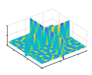
  $\omega ^*_z$ and contributed negatively by vorticity tilting and outflow intensification. Then we extend the theory to the equilibrium stage by accounting for the eddy-induced vertical shear, a stochastic factor that breaks the vertical coherency and terminates the outflow intensification. The flow fields at the two stages are demonstrated in figure 1, as well as in movies 1 and 2 in the supplementary material (available at https://doi.org/10.1017/jfm.2024.571).

Figure 1. Cross-sections of vertical vorticity normalized by  $f$ at (a) the convective onset stage and (b) the equilibrium stage. The data of the Ra3 experiment (see table 1) with stress-free boundaries are used (
 $\widetilde {{Ra}}=23.2$ and
  ${E}=10^{-4}$). The plots are of
  $\omega _z^*/f$ at the non-dimensional times (a)
  $t=8$ and (b)
  $t=100$. The horizontal plane is at
  $z=0.2$, and the vertical planes are at
  $x=1.25$ and
  $y=1.25$. The simulation domain is doubly periodic, with
  $0< x<2.5$,
  $0< y<2.5$ and
  $0< z<1$. See § 2 for the experimental setting and the non-dimensionalization procedure.
The paper is organized as follows. Section 2 introduces the governing equation and DNS set-up. Section 3 presents the  $S$ and
  ${Ro_g}$ diagnosed from DNS. Section 4 uses vertical mode decomposition and an asymptotic equation set to study
  $S$ at the convective onset stage. Section 5 extends the theory to the equilibrium stage. Section 6 concludes the research.
2. The governing equations and DNS set-up
This section introduces the variables, the governing equations and the DNS set-up. The dimensional variables (not including constant quantities) are denoted with *. Here,  $\boldsymbol {i}, \boldsymbol {j}, \boldsymbol {k}$ are the unit vectors of the Cartesian coordinates,
  $\boldsymbol {x}^*=(x^*,y^*,z^*)$ is the position,
  $\boldsymbol {u}^*=(u^*,v^*,w^*)$ is the velocity,
  $p^*$ is the pressure potential,
  $T^{*}$ is the perturbation temperature that has subtracted a diffusive-equilibrium linear temperature profile, and
  $\boldsymbol {\omega }^*=({\omega }_x^*,{\omega }_y^*,{\omega }_z^*)$ is the vorticity, with
  $\boldsymbol {\omega }^*=\boldsymbol {{\nabla }}^* \times \boldsymbol {u}^*$, where
  $\boldsymbol {\nabla }^* \equiv \boldsymbol {i}\,\partial /\partial x^* +\boldsymbol {j}\,\partial /\partial y^* + \boldsymbol {k}\, \partial /\partial z^*$ is the gradient operator. We non-dimensionalize the variables in the formulation of Portegies et al. (Reference Portegies, Kunnen, van Heijst and Molenaar2008). The convective overturning time scale is
  $H/W$, where the characteristic vertical velocity
  $W$ uses the free-fall scaling
  $W=\sqrt {g\beta \,{\Delta } T\,H}$. The length scale is the domain height
  $H$. The temperature scale is the temperature difference between the lower and upper plates,
  ${\Delta }T$. So
 \begin{equation} \left.\begin{gathered} t^*=t H/W,\quad {(x^*,y^*,z^*)}={(x,y,z)}\,H, \quad \boldsymbol{u}^*=\boldsymbol{u} W, \\ \boldsymbol{\omega}^*=\boldsymbol{\omega}W/H, \quad T^{*}= T\,\Delta T, \quad p^*=p W^2. \end{gathered}\right\} \end{equation}
 The convection is between a warm plate at  $z=0$ and a cold plate at
  $z=1$, with a doubly periodic lateral boundary. The flow obeys the incompressible Boussinesq equation:
 $$\begin{gather} \frac{\partial \boldsymbol{u}}{\partial t}+\left(\boldsymbol{u} \boldsymbol{\cdot}\boldsymbol{\nabla} \right)\boldsymbol{u}+\frac{1}{{Ro}}\,\boldsymbol{k} \times \boldsymbol{u} =- \boldsymbol{\nabla} p + T \boldsymbol{k}+{\left(\frac{{Pr}}{{Ra}}\right)}^{1/2}{\nabla}^2 \boldsymbol{u}, \end{gather}$$
 $$\begin{gather}\frac{\partial T
}{\partial t}+\left(\boldsymbol{u}
\boldsymbol{\cdot}\boldsymbol{\nabla}\right) T -w=
{\left({Pr\,Ra}\right)}^{-1/2}\,{\nabla}^2 T,
\end{gather}$$
$$\begin{gather}\frac{\partial T
}{\partial t}+\left(\boldsymbol{u}
\boldsymbol{\cdot}\boldsymbol{\nabla}\right) T -w=
{\left({Pr\,Ra}\right)}^{-1/2}\,{\nabla}^2 T,
\end{gather}$$ $$\begin{gather}\boldsymbol{\nabla}\boldsymbol{\cdot}\boldsymbol{u}=0, \end{gather}$$
where  $\boldsymbol {\nabla }\equiv \boldsymbol {i}\,\partial /\partial x +\boldsymbol {j}\, \partial /\partial y + \boldsymbol {k}\,\partial /\partial z$ is the non-dimensional gradient operator, and
  ${Ro} \equiv {E}({Ra/Pr})^{1/2}= W/(\,fH)$ is the convective Rossby number that measures the relative strength of thermal forcing to the rotational effect (Julien et al. Reference Julien, Legg, McWilliams and Werne1996b). Note that both
  ${Ro}$ and
  $\widetilde {{Ra}}\equiv {Ra}\,{E}^{4/3}$ are combinations of
  ${Ra}$ and
  ${E}$, but their physical interpretations are different:
  ${Ro}$ measures the deviation from geostrophic balance at the equilibrium state, and
  $\widetilde {{Ra}}$ measures the deviation from neutral stability (
 $\widetilde {{Ra}}\approx 8.7$; Chandrasekhar Reference Chandrasekhar1953). For the weakly nonlinear and rapidly rotating RRBC, there is
  ${Ro} \ll 1$ and
  $\widetilde {{Ra}} \lesssim O(10^1)$.
The temperature boundary condition is Dirichlet:
 \begin{equation} T |_{z=0}=0,\quad T |_{z=1}=0. \end{equation}
The impermeable velocity boundary condition is
 \begin{equation} \boldsymbol{k} \boldsymbol{\cdot}\boldsymbol{u}|_{z=0}=0,\quad \boldsymbol{k} \boldsymbol{\cdot} \boldsymbol{u}|_{z=1} =0. \end{equation}
For the tangential velocity, we study only the stress-free boundary condition:
 \begin{equation} \boldsymbol{k} \times \left.\frac{\partial \boldsymbol{u}}{\partial z}\right|_{z=0}=0, \quad \boldsymbol{k} \times \left.\frac{\partial \boldsymbol{u}}{\partial z}\right|_{z=1}=0. \end{equation}
 The DNS are performed with the Boussinesq solver of Cloud Model 1, version 19.8 (CM1; Bryan & Fritsch Reference Bryan and Fritsch2002). See Appendix A for the detailed numerical setting. The simulation is run in a  $[0,2.5]\times [0,2.5]\times [0,1]$ horizontally doubly periodic domain. The initial condition is a spatially uncorrelated random noise on
  $T$ in the whole domain, obeying a uniform distribution between
  $-0.25$ and
  $0.25$. This noise generation method is the default setting of the configured ‘Rayleigh–Bénard convection’ set-up in CM1. The perturbation amplitude uses the default value, which is relatively large but does not cause numerical instability in our simulations. We fix
  ${Pr}=1$, which is close to the
  ${Pr}\approx 0.7$ value of air and is mathematically simple (e.g. Vélez-Pardo & Cronin Reference Vélez-Pardo and Cronin2023). Because our
  $Pr$ is above 0.68, the primary instability is stationary, with vortices growing at the same location (Chandrasekhar Reference Chandrasekhar1953).
We define the convective onset stage as the stage where the vortices have not been sufficiently deformed and tilted by mutual advection or by any secondary instability (e.g. Küppers & Lortz Reference Küppers and Lortz1969; Carton Reference Carton1992). Practically, the end of the convective onset stage is set as the overshooting peak of the time series of  ${Ro_g}$, which marks the initiation of vortex interaction that breaks down the stationary pattern.
We perform two groups of experiments, with eight simulations in each group.
(i) Changing
 ${Ra}$ and using a fixed ${E}=10^{-4}$.
(ii) Changing
${E}$ and using a fixed ${Ra}=2.5\times 10^{6}$.


The experimental parameters are listed in table 1 and plotted in figure 2. We explore the parameter space around  ${Ra}=2.5\times 10^6$ and
  ${E}=10^{-4}$, because this point has been investigated carefully by Portegies et al. (Reference Portegies, Kunnen, van Heijst and Molenaar2008), and detailed background information is available. The critical Rayleigh number
  ${Ra_c}$ for the stress-free boundary case has an asymptotic expression:
  ${Ra_c} = 8.6956 (1-1.108{E}^{1/6} + 0.1533 {E}^{1/3}) {E^{-4/3}}$, derived by Homsy & Hudson (Reference Homsy and Hudson1971). The ratio
  ${Ra}/{Ra_c}$, which is a more accurate measure of supercriticality than
  $\widetilde {{Ra}}$, ranges from 1.52 to 16.30 in the experiments. The equilibrium states of our experiments are mainly in the cellular regime (
 $\widetilde {{Ra}}\lesssim 25$; Stellmach et al. Reference Stellmach, Lischper, Julien, Vasil, Cheng, Ribeiro, King and Aurnou2014).
Table 1. Values of  ${Ra}$,
  ${E}$,
  ${Ro \equiv E(}{{Ra/Pr)}}^{{1/2}}$,
  $\widetilde {{Ra}} \equiv {Ra}\,{{E}}^{{4/3}}$, and
  ${Ra}/{Ra_c}$ in the 16 numerical experiments. The
  ${Pr}$ value is fixed at 1. Note that Ra7 and E7 are identical.


Figure 2. The  ${E}$–
 ${Ra}$ parameter space investigated in this paper. The blue crosses denote experiments Ra1–Ra8. The red crosses denote experiments E1–E8. The black line denotes the critical Rayleigh number
  ${Ra_c}$ derived by Homsy & Hudson (Reference Homsy and Hudson1971).
The time interval of data output is  $0.5$. The total simulation length is 120, which goes through the convective onset stage and finally reaches a statistically equilibrium stage. Before calculating any quantity, the data are interpolated from the vertically stretched mesh to a vertically uniform mesh with 300 layers using the cubic spline function. The motivation for the interpolation is to facilitate the calculation of numerical integral and finite difference. As readers will see,
  $S$ calculated with the interpolated data converges to zero in the
  ${Ro_g} \to 0$ limit, so the interpolation error should be negligible.
3. Simulation results
Unlike previous studies that investigate the vorticity skewness at different heights (Julien et al. Reference Julien, Legg, McWilliams and Werne1996b; Kunnen et al. Reference Kunnen, Geurts and Clercx2009), we investigate the contribution from different vertical eigenmodes. Vertical mode decomposition is a useful technique in studying linear and weakly nonlinear waves in a vertically confined domain (e.g. Vallis Reference Vallis2017). To our knowledge, it has not been applied to analyse the vorticity skewness in RRBC. For RRBC with stress-free boundary conditions, the vertical eigenfunction is the trigonometric function:
 \begin{equation} \sin(n{\rm \pi} z)\quad\text{and}\quad\cos(n{\rm \pi} z),\quad n=0,1,2,\ldots. \end{equation}
The  $n=0$ mode is called the barotropic mode, and
  $n\geq 1$ modes are called baroclinic modes. Variables with the Dirichlet and Neumann boundary conditions take the
  $\sin (n{\rm \pi} z)$ and
  $\cos (n{\rm \pi} z)$ shapes, respectively. Thus
  $u$,
$u$,  $v$,
$v$,  $\omega _z$,
  $p$ have a vertical structure of
  $\cos ( n {\rm \pi}z )$, and
  $w$,
$w$,  $T$,
$T$,  $\boldsymbol {\omega }_h$ (horizontal vorticity vector) have a vertical structure of
  $\sin ( n {\rm \pi}z )$.
In this section, we do not distinguish between baroclinic modes and simply decompose  $\omega _z$ into the barotropic mode and a bulk baroclinic mode. The barotropic mode is simply the vertical average of
  $\omega _z$, defined as
  $\overline {\omega _z}$. The baroclinic mode is the vertical anomaly, defined as
  $\omega '_z$. Because only the baroclinic modes can be linearly unstable,
  $\overline {\omega _z}$ must be nonlinearly generated by baroclinic modes, and there should be
  $O(\overline {\omega _z}) \ll O(\omega '_z)$ in the weakly nonlinear regime. Substituting
  $\omega _z = \overline {\omega _z} + \omega '_z$ into (1.2a–c), we decompose
  $S$ into the barotropic contribution, the baroclinic contribution and the barotropic–baroclinic contribution:
 \begin{align} S &= \overbrace{ \frac{
\langle \overline{ \overline{\omega_z}^3 } \rangle
}{\langle \overline{\omega^2_z} \rangle^{3/2} }
}^{\textit{barotropic}} + \overbrace{ \frac{ \langle
\overline{ {\omega'_z}^3 } \rangle }{\langle
\overline{\omega^2_z} \rangle^{3/2} } }^{\textit{baroclinic}}
+ \overbrace{ 3\,\frac{ \langle \overline{
\overline{\omega_z}^2 {\omega'_z} } \rangle }{\langle
\overline{\omega^2_z} \rangle^{3/2} } + 3\,\frac{ \langle
\overline{ \overline{\omega_z} {\omega'_z}^2 } \rangle
}{\langle \overline{\omega^2_z} \rangle^{3/2} }
}^{\textit{barotropic--baroclinic}}
\nonumber\\ &\approx \frac{ \langle \overline{
{\omega'_z}^3 } \rangle }{\langle \overline{\omega^2_z}
\rangle^{3/2} } + 3\,\frac{ \langle \overline{
\overline{\omega_z} {\omega'_z}^2 } \rangle }{\langle
\overline{ \omega^2_z } \rangle^{3/2} }.
\end{align}
\begin{align} S &= \overbrace{ \frac{
\langle \overline{ \overline{\omega_z}^3 } \rangle
}{\langle \overline{\omega^2_z} \rangle^{3/2} }
}^{\textit{barotropic}} + \overbrace{ \frac{ \langle
\overline{ {\omega'_z}^3 } \rangle }{\langle
\overline{\omega^2_z} \rangle^{3/2} } }^{\textit{baroclinic}}
+ \overbrace{ 3\,\frac{ \langle \overline{
\overline{\omega_z}^2 {\omega'_z} } \rangle }{\langle
\overline{\omega^2_z} \rangle^{3/2} } + 3\,\frac{ \langle
\overline{ \overline{\omega_z} {\omega'_z}^2 } \rangle
}{\langle \overline{\omega^2_z} \rangle^{3/2} }
}^{\textit{barotropic--baroclinic}}
\nonumber\\ &\approx \frac{ \langle \overline{
{\omega'_z}^3 } \rangle }{\langle \overline{\omega^2_z}
\rangle^{3/2} } + 3\,\frac{ \langle \overline{
\overline{\omega_z} {\omega'_z}^2 } \rangle }{\langle
\overline{ \omega^2_z } \rangle^{3/2} }.
\end{align}
The purely barotropic contribution  ${ \langle \overline { \overline {\omega _z}^3 } \rangle }/{\langle \overline {\omega ^2_z} \rangle ^{3/2}}$ is negligible because
  $O(\overline {\omega _z}) \,{\ll}\, O(\omega '_z)$. The
  $3({ \langle \overline { \overline {\omega _z}^2 {\omega '_z} } \rangle }/{\langle \overline {\omega ^2_z} \rangle ^{3/2} })$ term equals zero because
  $3 ({ \langle \overline { \overline {\omega _z}^2 {\omega '_z} } \rangle }/{\langle \overline {\omega ^2_z} \rangle ^{3/2} }) = 3( { \langle \overline {\omega _z}^2 \overline { {\omega '_z} } \rangle }/ \langle \overline {\omega ^2_z} \rangle ^{3/2}) =0$, where we have used
  $\overline {\omega '_z}=0$. This simplification is validated with DNS (figures 3 and 4). The only two terms remaining are the purely baroclinic term
  ${ \langle \overline { {\omega '_z}^3 } \rangle }/{\langle \overline {\omega ^2_z} \rangle ^{3/2} }$ and the barotropic–baroclinic term
  $3 ({ \langle \overline { \overline {\omega _z} {\omega '_z}^2 } \rangle }/{\langle \overline { \omega ^2_z } \rangle ^{3/2} })$. Figures 3(e–h) and 4(e–h) show that at the convective onset stage, the purely baroclinic term is negative, and the barotropic–baroclinic term is positive. The magnitude of the former is approximately half of the latter, except for the Ra1 and E1 experiments that have relatively large
  $\widetilde {{Ra}}$ and
  ${Ro}$.

Figure 3. (a–d) The time evolution of the vorticity skewness  $S \equiv { \langle \overline { \omega ^3_z } \rangle }/{\langle \overline { \omega ^2_z } \rangle ^{3/2} }$ (black line) and its decomposed parts. The blue line shows
  ${ \langle \overline { \overline {\omega }^3_z } \rangle }/{\langle \overline {\omega ^2_z} \rangle ^{3/2} }$, the red line shows
  ${ \langle \overline { {\omega '_z}^3 } \rangle }/{\langle \overline {\omega ^2_z} \rangle ^{3/2} }$, the yellow line shows
  $3({ \langle \overline { \overline {\omega _z}^2 {\omega '_z} } \rangle }/{\langle \overline {\omega ^2_z} \rangle ^{3/2} })$, and the purple line shows
  $3 ({ \langle \overline { \overline {\omega _z} {\omega '_z}^2 } \rangle }/{\langle \overline {\omega ^2_z} \rangle ^{3/2} })$. The blue shading marks the convective onset stage, which ends at the time of maximum
  ${Ro_g}$. The red shading marks the equilibrium stage, which is between
  $t=90$ and
  $t=120$, and will be studied in § 5. The four plots are for experiments (a) Ra1, (b) Ra3, (c) Ra5, and (d) Ra8. (e–h) Comparison of the purely baroclinic term
  ${ \langle \overline { {\omega '_z}^3 } \rangle }/{\langle \overline {\omega ^2_z} \rangle ^{3/2} }$ and the barotropic– baroclinic term
  $3 ({ \langle \overline { \overline {\omega _z} {\omega '_z}^2 } \rangle }/{\langle \overline {\omega ^2_z} \rangle ^{3/2} })$, with the colour of the dots denoting time (
 $0< t<20$, from blue to yellow). The time interval between two dots is 0.5. For (e), only a small portion of data points lie in the scope of plotting. The solid black line is the
  $2:-1$ reference line. Here, (a,e)
  $\widetilde {Ra}=58.0$, (b,f)
  $\widetilde {Ra}=23.2$, (c,g)
  $\widetilde {Ra}=14.5$, and (d,h)
  $\widetilde {Ra}=10.5$.

Figure 4. The same as figure 3, but for experiments E1, E3, E5 and E8 that change  ${E}$ and fix
  ${Ra}$. For (e,f), only a small portion of data points lie in the scope of plotting. Here, (a,e)
  $E=5.00\times 10^{-4}$, (b,f)
  $E=2.50\times 10^{-4}$, (c,g)
  $E=1.67\times 10^{-4}$, and (d,h)
  $E=9.09\times 10^{-5}$.
Equation (3.2) indicates that the skewness originates from the correlation between the baroclinic or barotropic vorticity with  $\omega '^2_z$. The region with a high
  $\omega '^2_z$ is essentially the rich-vorticity region. We define the lines crossing the centre of the rich-vorticity region as the vortex axes. At the convective onset stage, they coincide with the axes of strongest vertical motions. Therefore, the vorticity structure along the vortex axis is crucial for modelling the skewness.
Figures 5 and 6 show  $S \propto {Ro}_{{g}}$ for almost all simulations, with proportional factor approximately 2.5. The exceptions are the Ra1 and E1 experiments, where the
  ${Ro}\ll 1$ and
  $\widetilde {{Ra}} \lesssim O(10^1)$ conditions are violated. Note that
  ${Ro_g}$ and
  ${Ro}$ have different physical meanings:
  ${Ro_g}$ is a diagnostic quantity that represents the instantaneous vorticity amplitude, while
  ${Ro}$ is an a priori estimation of
  ${Ro_g}$ at the equilibrium state. Section 4 focuses on the convective onset stage. We use asymptotic analysis and vertical mode decomposition to derive a Galerkin model, which proves
  $S \propto {Ro_g}$ and explains why the barotropic–baroclinic and purely baroclinic terms make opposite contributions to
  $S$. They are the basis for understanding the more complicated equilibrium stage in § 5.

Figure 5. The dots show the dependence of the volumetric vorticity skewness  $S$ on the global Rossby number
  ${Ro_{g}}$ during
  $0< t<20$. The data sampling time interval is 0.5. (a–h) Plots for experiments Ra1–Ra8 with a fixed
  ${E}=10^{-4}$. The colour of the dots denotes time (
 $0< t<20$, from blue to yellow). The solid black lines show the
  $S = 2.5 {Ro_g}$ fitting relation. Here, (a)
  $\widetilde {Ra}=58.0$, (b)
  $\widetilde {Ra}=38.7$, (c)
  $\widetilde {Ra}=23.2$, (d)
  $\widetilde {Ra}=16.6$, (e)
  $\widetilde {Ra}=14.5$, (f)
  $\widetilde {Ra}=12.2$, (g)
  $\widetilde {Ra}=11.6$, and (h)
  $\widetilde {Ra}=10.5$.

Figure 6. The same as figure 6, but for experiments E1–E8 that change  ${E}$ and fix
  ${Ra}$: (a)
  $E=5.00\times 10^{-4}$, (b)
  $E=3.33\times 10^{-4}$, (c)
  $E=2.50\times 10^{-4}$, (d)
  $E=2.00\times 10^{-4}$, (e)
  $E=1.67\times 10^{-4}$, (f)
  $E=1.25\times 10^{-4}$, (g)
  $E=1.00\times 10^{-4}$, and (h)
  $E=9.09\times 10^{-5}$.
4. The vorticity skewness at the convective onset stage
4.1. Vertical mode decomposition
This subsection studies what controls  $S$ at the convective onset stage. The main idea is to perform a vertical mode decomposition, and study the contribution from each mode. We decompose velocity
  $(u,v,w)$, horizontal vorticity
  $\boldsymbol {\omega }_h$, vertical vorticity
  $\boldsymbol {\omega }_z$, pressure
  $p$, and temperature
  $T$ into different vertical modes:
 \begin{equation} \left.\begin{gathered} u = u_0 + u_1 + u_2 +\cdots, \\ v = v_0 + v_1 + v_2 +\cdots, \\ w = w_0 + w_1 + w_2 +\cdots, \\ \boldsymbol{\omega}_h=\boldsymbol{\omega}_{h,0} +\boldsymbol{\omega}_{h,1}+ \boldsymbol{\omega}_{h,2} +\cdots, \\ \omega_z = \omega_{z,0} + \omega_{z,1} + \omega_{z,2} +\cdots, \\ p = p_0 + p_1 + p_2 +\cdots, \\ T = T_0 + T_1 + T_2 +\cdots, \end{gathered}\right\} \end{equation}
where the subscript  $n$ denotes the
  $n\textrm {th}$ vertical mode, with vertical structure
  $\sin (n {\rm \pi}z)$ or
  $\cos (n {\rm \pi}z)$. For the weakly nonlinear regime, only the
  $n=1$ mode is susceptible to linear instability, so the
  $n=0$ and
  $n=2$ modes are driven nonlinearly by the
  $n=1$ quantities. Thus the
  $n=0$ and
  $n=2$ modes are smaller than the
  $n=1$ modes by an order of
  ${Ro}$ (strictly speaking,
  ${Ro_g}$). The
  $n \geq 3$ modes are higher-order nonlinear effects neglected in this analysis.
We express the third-order moment of vorticity, which is the numerator of  $S$, with the
  $n=0, 1, 2$ modes:
 \begin{align} \left \langle \overline{\omega^3_z} \right \rangle & \approx \left \langle \overline{ \left( \omega_{z,0} +\omega_{z,1} +\omega_{z,2} \right)^3 } \right \rangle \nonumber\\ &= \langle \overline{\omega^3_{z,0}} + \overline{\omega^3_{z,1}} + \overline{\omega^3_{z,2}} \rangle + 6 \langle \overline{\omega_{z,0} \omega_{z,1} \omega_{z,2}} \rangle \nonumber\\ &\quad + 3 \langle \overline{\omega^2_{z,0} \omega_{z,1}} + \overline{\omega_{z,0} \omega^2_{z,1}} + \overline{\omega^2_{z,0} \omega_{z,2}} + \overline{\omega_{z,0} \omega^2_{z,2}} + \overline{\omega^2_{z,1} \omega_{z,2}} + \overline{\omega_{z,1} \omega^2_{z,2}}\rangle \nonumber\\ &\approx 3 \langle \overline{\omega^2_{z,1} \omega_{z,0}} \rangle + 3 \langle \overline{\omega^2_{z,1} \omega_{z,2}} \rangle. \end{align}
The first term of the fourth line is essentially the  $3 \langle \overline { \overline {\omega _z} {\omega '_z}^2 } \rangle$ term in (3.2), and the second term is essentially the
  $\langle \overline { {\omega '_z}^3 } \rangle$ term. Many terms have been neglected, as explained below. Some terms are exactly zero:
 \begin{equation} \left.\begin{gathered} \langle \overline{ \omega^3_{z,1} } \rangle \propto \overline{\cos^3 \left( {\rm \pi}z \right)}=0, \quad 6 \langle \overline{\omega_{z,0} \omega_{z,1} \omega_{z,2}} \rangle \propto \overline{\cos \left( {\rm \pi}z \right) \cos \left( 2 {\rm \pi}z \right) }=0,\\ 3 \langle \overline{\omega^2_{z,0} \omega_{z,1}} \rangle \propto \overline{ \cos \left( {\rm \pi}z \right) }=0, \quad 3 \langle \overline{\omega^2_{z,0} \omega_{z,2}} \rangle \propto \overline{ \cos \left( 2 {\rm \pi}z \right) }=0,\\ 3 \langle \overline{\omega_{z,1} \omega^2_{z,2}} \rangle \propto \overline{ \cos \left( {\rm \pi}z \right) \cos^2 \left( 2 {\rm \pi}z \right) }=0. \end{gathered}\right\} \end{equation}
The rest of the neglected terms, i.e.  $\langle \overline {\omega ^3_{z,0}} \rangle$,
  $\langle \overline {\omega ^3_{z,2}} \rangle$ and
  $3 \langle \overline {\omega _{z,0} \omega ^2_{z,2}} \rangle$, are order
  ${Ro}^2$ smaller than the retained terms. This section is devoted to understanding the relationship between
  $\omega _{z,0}$,
  $\omega _{z,1}$ and
  $\omega _{z,2}$, which involves the full coupling between dynamical and thermodynamic processes.
4.2. A Galerkin model
We derive a Galerkin model of  $n=0, 1, 2$ modes from a simplified set of equations. As a simplification from Veronis (Reference Veronis1959), we apply two assumptions that work for the rapidly rotating and weakly nonlinear regime.
(i) The divergence equation uses geostrophic balance, which requires
${Ro} \ll 1$. This assumption is crucial for deriving the quasi-geostrophic omega equation in § 4.3, which helps us to understand the origin of $S$.(ii) The
$n=1$ mode is the only unstable vertical mode, which requires $8.7 \lesssim \widetilde{{Ra}} \lesssim 21.9$. This is because the critical $\widetilde {{Ra}}$ of the $n$th mode in the rapidly rotating limit approximately obeys $8.7 n^{4/3}$ (Chandrasekhar Reference Chandrasekhar1953). We take it as $\widetilde {{Ra}} \lesssim 20$ for simplicity.


A natural consequence of the two assumptions is  ${E}={Ro}^3\, \widetilde {{Ra}}^{-3/2}\,{Pr}^{3/2} \ll 1$. Because the most unstable horizontal total wavenumber is
  $K_m = ({\rm \pi} ^2/2)^{1/6} {E}^{-1/3}$, we must have
  $K_m \gg 1$, and the vortices must have a small width-to-depth ratio (Chandrasekhar Reference Chandrasekhar1953). This allows us to neglect viscosity and thermal diffusion in the vertical direction. The simplified governing equation set is shown below, with linear terms on the left-hand side and nonlinear terms on the right-hand side:
 $$\begin{gather} \left( \frac{\partial}{\partial t} - {Ra}^{-1/2}\,\nabla_h^2 \right) \omega_z - \frac{1}{{Ro}}\,\frac{\partial w}{\partial z} =- \boldsymbol{u} \boldsymbol{\cdot}\boldsymbol{\nabla}\omega_z + \boldsymbol{\omega} \boldsymbol{\cdot}\boldsymbol{\nabla} w, \end{gather}$$
 $$\begin{gather}\nabla^2_h p - \frac{1}{{Ro}}\,\omega_z = 0, \end{gather}$$
 $$\begin{gather}\left( \frac{\partial}{\partial t} - {Ra}^{-1/2}\,\nabla_h^2 \right) w + \frac{\partial p}{\partial z} - T =- \boldsymbol{u}\boldsymbol{\cdot}\boldsymbol{\nabla}w, \end{gather}$$
 $$\begin{gather}\left( \frac{\partial}{\partial t} - {Ra}^{-1/2}\,\nabla_h^2 \right) T =- \boldsymbol{u}\boldsymbol{\cdot}\boldsymbol{\nabla}T, \end{gather}$$
 $$\begin{gather}\boldsymbol{\nabla}\boldsymbol{\cdot}\boldsymbol{u} = 0, \end{gather}$$
where  $\boldsymbol {\nabla }_h \equiv \boldsymbol {i}\,\partial /\partial x +\boldsymbol {j}\,\partial /\partial y$ denotes the horizontal gradient. Equation (4.5) is the divergence equation using the geostrophic balance approximation. Also, note the
  $\nabla ^2 \approx \nabla ^2_h$ approximation used in the viscosity and diffusion terms.
The simplified equation set is similar to yet different from the non-hydrostatic quasi-geostrophic (NHQG) equation proposed by Sprague et al. (Reference Sprague, Julien, Knobloch and Werne2006), which is derived in the regime of  ${Ro} \ll 1$ and small width-to-depth ratio, using multiple time scale asymptotic expansion. The rigorous NHQG equation yields zero
  $S$. We retain a few terms neglected in the NHQG scaling, which are crucial for generating vorticity asymmetry.
(i) In the vertical vorticity equation (4.4), the advection of
$\omega _z$ by the toroidal velocity, the stretching of $\omega _z$, and tilting terms are retained. The toroidal velocity includes the vertical velocity and the curl-free component of horizontal velocity.(ii) In the
$w$ equation (4.6), the advection of $w$ by the toroidal velocity is retained.(iii) In the
$T$ equation (4.7), the advection of perturbation temperature $T$ by the toroidal velocity is retained. This term is partially represented in the NHQG equation by allowing the horizontally averaged temperature perturbation $\langle T \rangle$ evolve.


We will show that factor (i) contributes positively to  $S$, and factors (ii) and (iii) contribute negatively to
  $S$, at the convective onset stage. Substituting (4.1) into the simplified equation set (4.4)–(4.8), we obtain a Galerkin model of the
  $n=1$,
  $n=2$ and
  $n=0$ modes relevant for calculating skewness.
The  $n=1$ mode equation is
 $$\begin{gather} \left( \frac{\partial}{\partial t} - {Ra}^{-1/2}\,\nabla_h^2 \right) \omega_{z,1} - \frac{1}{{Ro}}\,\frac{\partial w_1}{\partial z} = 0, \end{gather}$$
 $$\begin{gather}\nabla^2_h p_1 - \frac{1}{{Ro}}\,\omega_{z,1}= 0, \end{gather}$$
 $$\begin{gather}\left( \frac{\partial}{\partial t} - {Ra}^{-1/2}\,\nabla_h^2 \right) w_1 + \frac{\partial p_1}{\partial z} - T_1 = 0, \end{gather}$$
 $$\begin{gather}\left( \frac{\partial}{\partial t} - {Ra}^{-1/2}\,\nabla_h^2 \right) T_1 - w_1 = 0, \end{gather}$$
 $$\begin{gather}\boldsymbol{\nabla}\boldsymbol{\cdot}\boldsymbol{u}_1 = 0. \end{gather}$$
The eigenvalue of the  $n=1$ equation is the growth rate
  $\sigma$ of the linear instability:
 \begin{equation} \sigma = \left( \frac{K^2 - {Ro}^{-2}\,{\rm \pi}^2}{K^2} \right)^{1/2} - {Ra}^{-1/2}\,K^2. \end{equation}
 The  $n=2$ mode governing equation is
 $$\begin{gather} \left( \frac{\partial}{\partial t} - {Ra}^{-1/2}\,\nabla_h^2 \right) \omega_{z,2} - \frac{1}{{Ro}}\,\frac{\partial w_2}{\partial z} = 0, \end{gather}$$
 $$\begin{gather}\nabla^2_h p_2 - \frac{1}{{Ro}}\,\omega_{z,2} = 0, \end{gather}$$
 $$\begin{gather}\left( \frac{\partial}{\partial t} - {Ra}^{-1/2}\,\nabla_h^2 \right) w_2 + \frac{\partial p_2}{\partial z} - T_2 =- \boldsymbol{u}_1 \boldsymbol{\cdot} \boldsymbol{\nabla} w_1, \end{gather}$$
 $$\begin{gather}\left( \frac{\partial}{\partial t} - {Ra}^{-1/2}\,\nabla_h^2 \right) T_2 - w_2 =- \boldsymbol{u}_1 \boldsymbol{\cdot}\boldsymbol{\nabla} T_1, \end{gather}$$
 $$\begin{gather}\boldsymbol{\nabla}\boldsymbol{\cdot}\boldsymbol{u}_2 = 0. \end{gather}$$
 For the  $n=0$ mode, only the vertical vorticity equation is needed:
 \begin{align} \left( \frac{\partial}{\partial t} - {Ra}^{-1/2}\,\nabla_h^2 \right) \omega_{z,0} &=- \underbrace{ w_1\,\frac{\partial \omega_{z,1}}{\partial z} }_{\textit{vertical advection}} + \underbrace{\omega_{z,1}\,\frac{\partial w_1}{\partial z}}_{\textit{stretching}} \nonumber\\ &\quad - \underbrace{ \left( \boldsymbol{u}_1 \boldsymbol{\cdot} \boldsymbol{\nabla}_h \right) \omega_{z,1} }_{\textit{horizontal advection}} + \underbrace{\left( \boldsymbol{\omega}_{h,1} \boldsymbol{\cdot} \boldsymbol{\nabla}_h \right) w_1 }_{\textit{tilting}}. \end{align}
The stretching of solid-body vorticity cannot produce barotropic vorticity because the barotropic mode is purely two-dimensional. We call the right-hand side terms of (4.20) ageostrophic effects because they do not exist in the NHQG scaling (Sprague et al. Reference Sprague, Julien, Knobloch and Werne2006).
The Galerkin model has been greatly simplified by the assumption that the instability is dominated by a single mode with a unique horizontal and vertical wavenumber. The  $- \boldsymbol {u}_1 \boldsymbol {\cdot } \boldsymbol {\nabla } w_1$ and
  $- \boldsymbol {u}_1 \boldsymbol {\cdot } \boldsymbol {\nabla } T_1$ terms only project onto the
  $n=2$ mode:
 \begin{equation} - \boldsymbol{u}_1 \boldsymbol{\cdot} \boldsymbol{\nabla} w_1,\ - \boldsymbol{u}_1 \boldsymbol{\cdot} \boldsymbol{\nabla} T_1 \propto \sin ( {\rm \pi}z ) \cos ( {\rm \pi}z ) \sim \sin ( 2 {\rm \pi}z ). \end{equation}
The sum of the vertical advection and stretching of  $\omega _{z,1}$ only projects onto the
  $n=0$ mode vorticity equation:
 \begin{equation} - w_1\,\frac{\partial \omega_{z,1}}{\partial z} + \omega_{z,1}\,\frac{\partial w_1}{\partial z} \propto \sin^2 ( {\rm \pi}z ) + \cos^2 ( {\rm \pi}z ) \sim 1. \end{equation}
In Appendix B, we prove that with an additional axisymmetric assumption, which approximately works for vortices at the convective onset stage, the sum of the horizontal advection and tilting terms also only project onto the  $n=0$ mode vorticity equation.
Next, we study the two parts of  $S$, which is from the interaction between the
  $n=1$ and
  $n=2$ modes, and from the interaction between the
  $n=1$ and
  $n=0$ modes:
 \begin{equation} S\approx 3\,\frac{\langle \overline{\omega^2_{z,1} \omega_{z,2} } \rangle}{ \langle \overline{\omega^2_{z,1}} \rangle^{3/2} } + 3\,\frac{\langle \overline{ {\omega^2_{z,1}} \omega_{z,0} } \rangle}{ \langle \overline{\omega^2_{z,1}} \rangle^{3/2} }. \end{equation}
Note that the self-interaction of the  $n=1$ mode does not generate vorticity skewness, because
  $\langle \overline { \omega ^3_{z,1} } \rangle =0$, as shown in (4.3).
4.3. The negative contribution to $S$ from the $n=2$ mode


The  $n=2$ vertical vorticity equation (4.15) has an intriguing property: it is linear. Thus
  $\omega _{z,2}$ is only driven by the stretching of solid-body vorticity by
  $w_2$. The quasi-geostrophic approximation on the divergence equation (4.16) allows us to derive the diagnostic equation of
  $w_2$, essentially the quasi-geostrophic omega equation (e.g. Holton Reference Holton2004) in the non-hydrostatic state with unstable stratification. Combining (4.15)–(4.19), we obtain
 \begin{align} &\left[ \underbrace{ \frac{1}{{Ro}^2}\,\frac{\partial^2}{\partial z^2} }_{\textit{from}\ p_2,\,<0} \underbrace{ - \nabla^2_h }_{\textit{from}\ T_2\ \textit{adv},\,>0} + \underbrace{ \left( \frac{\partial}{\partial t} - {Ra}^{-1/2}\,\nabla_h^2 \right)^2 \nabla_h^2}_{\textit{non-hydrostatic},\,<0} \right] w_2 \nonumber\\ &\quad =- \left( \frac{\partial}{\partial t} - {Ra}^{-1/2}\,\nabla_h^2 \right) \nabla_h^2 \left( \boldsymbol{u}_1 \boldsymbol{\cdot}\boldsymbol{\nabla} w_1 \right) - \nabla_h^2 \left( \boldsymbol{u}_1 \boldsymbol{\cdot}\boldsymbol{\nabla} T_1 \right). \end{align}
The operator on the left-hand side includes three important terms.
(i) The pressure gradient part
$({1}/{{Ro}^2})({\partial ^2}/{\partial z^2})$, which suppresses $w_2$. This is because convergence produces a cyclone and therefore a low-pressure anomaly, and vice versa for divergence. Thus pressure gradient force always points from a divergent zone to a convergent zone, suppressing $w_2$.(ii) The temperature advection part
$\nabla _h^2$, which amplifies $w_2$. This term originates from the $w_2$ term in (4.18). It amplifies $w_2$ because a higher $w_2$ increases the buoyancy ($T_2$) and accelerates an updraft, and similarly for a downdraft. This term has an opposite sign in the traditional omega equation applied to a stably stratified fluid.(iii) The non-hydrostatic term, which suppresses
$w_2$.


The omega equation helps us to infer the trend of  $w_2$ from the forcing terms. First, we analyse the left-hand-side operator of (4.24). The first and third terms yield a multiplier with a minus sign, and the second term yields a positive sign. We can determine the sign of the left-hand-side operator without solving the omega equation. If the
  $n=1$ variables were substituted into the left-hand side operator,
 \begin{equation} n=1,\quad -\nabla^2_h=K_m^2, \quad \frac{\partial}{\partial t} = \sigma, \quad \frac{\partial^2}{\partial z^2}=-{\rm \pi}^2, \end{equation}
then the left-hand side would be zero, providing a reference. Now we substitute in the  $n=2$ variables (e.g.
  $w_2$). Because the right-hand-side forcing terms of (4.24) are product terms of the
  $n=1$ mode, we must have
  $\partial /\partial t=2\sigma$, and the horizontal structure of the
  $n=2$ mode must be approximately twice as fine-grained as the
  $n=1$ mode. Thus we set
  $-\nabla ^2_h \approx \alpha ^2 K^2_m$, where
  $\alpha$ is an unknown parameter, diagnosed to be
  $1<\alpha <2$ in Appendix C (figure 12). The vertical structure of the
  $n=2$ mode is also more fine-grained, yielding
  $\partial ^2/\partial z^2=-4{\rm \pi} ^2$. This is summarized as
 \begin{equation} n=2,\quad -\nabla^2_h \approx \alpha^2 K_m^2,\quad \frac{\partial}{\partial t} = 2 \sigma, \quad \frac{\partial^2}{\partial z^2}=-4{\rm \pi}^2. \end{equation}
Using (4.25a–c) and (4.26a–c), we calculate the change of magnitude of each left-hand-side term when switching from  $n=1$ to
  $n=2$:
 \begin{equation} \left.\begin{gathered} \frac{1}{{Ro}^2}\,\frac{\partial^2}{\partial z^2}\times 4, \\ - \nabla^2_h \times \alpha^2,\\ \left( \frac{\partial}{\partial t} - {Ra}^{-1/2}\,\nabla_h^2 \right)^2 \nabla_h^2 \times \underbrace{\frac{(2 \sigma + \alpha^2 {Ra}^{-1/2}\,K^2_m)^2 \alpha^2}{(\sigma+{Ra}^{-1/2}\,K^2_m)^2}}_{> \alpha^2}. \end{gathered}\right\} \end{equation}
Because  $1<\alpha <2$, the first and third terms of (4.27) are amplified more than the second term when switching from
  $n=1$ to
  $n=2$. Thus they dominate the sign of the left-hand-side operator, and the operator must correspond to a negative multiplier.
The above analysis shows that along the vortex axis,  $w_2$ must have the same sign as
  $-\boldsymbol {u}_1 \boldsymbol {\cdot } \boldsymbol {\nabla } w_1$ and
  $-\boldsymbol {u}_1 \boldsymbol {\cdot } \boldsymbol {\nabla } T_1$, which causes
  $w$ to deform downwind vertically. The downwind deformation denotes the shift of the zero divergence height towards the outflow zone, essentially an intensification of outflow (figure 7a). As a result, the convergent zone is more diluted than the divergent zone, making the magnitude of the cyclone produced by stretching the solid-body vorticity smaller than the magnitude of the anticyclone produced by squashing the solid-body vorticity. This explains why the
  $n=2$ mode contributes negatively to
  $S$.
$S$.

Figure 7. A schematic illustration of the vorticity skewness generation along the vortex axis at the convective onset stage. An updraft is used as an example. (a) The vertical velocity downwind deformation (outflow intensification) enhances the squashing of solid-body vorticity, generating a strong anticyclone (AC). It contributes negatively to  $S$ via the interaction between the
  $n=2$ and
  $n=1$ modes. (b) The vertical advection and stretching of
  $\omega _z$ produce a barotropic cyclone (CC) along the vortex axis. It contributes positively to
  $S$ via the interaction between the
  $n=0$ and
  $n=1$ modes. The solid blue lines denote (a) the
  $n=1$ mode vertical velocity and (b) the vertical vorticity profile along the vortex axes. The solid red lines denote (a) the bulk vertical velocity and (b) the vertical vorticity profile. The dashed black lines are zero-value reference lines.
Here are physical explanations for the downwind deformation. We take the updraft as an example. Here,  $-\boldsymbol {u}_1 \boldsymbol {\cdot } \boldsymbol {\nabla } w_1$ denotes the inertia of a parcel. Buoyancy remains positive along the air column, so the parcel keeps accelerating until steered to divergence near the upper plate, causing a downwind deformation of the vertical velocity profile. Meanwhile, the upward advection of temperature makes the temperature lapse rate smaller at the lower level and larger at the upper level. This reduces the low-level convective instability and enhances the upper-level convective instability. Thus the peak height of vertical velocity must shift to a higher level, also causing a downwind deformation. An extreme example of downwind deformation of vertical velocity is a buoyant plume, which keeps entraining (converging) fluids unless a ceiling forces it to diverge (e.g. Rooney & Linden Reference Rooney and Linden2012).
4.4. The positive contribution to $S$ from the $n=0$ mode


Equation (4.20) shows that along the vortex axis, the barotropic vorticity is produced by the vertical advection term  $-w_1({\partial \omega _{z,1}}/{\partial z})$ and the stretching term
  $\omega _{z,1}({\partial w_1}/{\partial z})$. For an updraft, there is a low-level cyclone and an upper-level anticyclone. The down-gradient advection produces an overall cyclonic anomaly. The stretching on the low-level cyclone and the squashing on the upper-level anticyclone produce an overall cyclonic anomaly. Thus both terms generate cyclonic anomaly along the vortex axis, producing a barotropic cyclone, as illustrated in figure 7(b). The cyclonic bias produced by these mechanisms has been identified in many previous studies of rotating fluids (e.g. Schubert & Alworth Reference Schubert and Alworth1987; Morize et al. Reference Morize, Moisy and Rabaud2005; Majda, Mohammadian & Xing Reference Majda, Mohammadian and Xing2008). The only discussion in the context of RRBC seems to be from Guervilly et al. (Reference Guervilly, Hughes and Jones2014). They explained the cyclonic bias as the concentration of cyclonic vorticity by the convergent flow and the dilution of anticyclonic vorticity by the divergent flow. It is an explanation based on the flux-form vorticity equation (e.g. Haynes & McIntyre Reference Haynes and McIntyre1987), consistent with the explanation based on the stretching of
  $\omega _z$.
Readers might ask: what is the role of the horizontal advection and tilting terms? They are zero along the vortex axis. Tory, Montgomery & Davidson (Reference Tory, Montgomery and Davidson2006) made a budget analysis of a simulated tropical cyclone precursor vortex. They found a core–shield structure of barotropic vorticity, with the horizontal advection and tilting terms producing an anticyclonic shield around a cyclonic core. The shield structure in the RRBC problem is theoretically confirmed in Appendix B and visible in the simulation result (figure 11(c) of Appendix C). Note that this shield is a nonlinearly generated depth-averaged structure that needs to be compared cautiously with the RRBC literature, where the shield (or sleeve) is more loosely defined as a ring of opposite-sign vorticity to the vortex core that is also seen in the linear instability (e.g. Sprague et al. Reference Sprague, Julien, Knobloch and Werne2006; Portegies et al. Reference Portegies, Kunnen, van Heijst and Molenaar2008; Grooms et al. Reference Grooms, Julien, Weiss and Knobloch2010; Shi et al. Reference Shi, Lu, Ding and Zhong2020). Because the anticyclonic shield renders  $\omega _{z,0}<0$, it produces negative vorticity skewness via
  $\langle \overline {\omega _{z,0} \omega ^2_{z,1}} \rangle$. However, because the shield is off the vortex axis, its negative contribution is minor compared to the positive contribution by vertical advection and stretching along the vortex axis. In fact, the bulk effect of the horizontal and vertical advection of
  $\omega _z$ does not produce volumetric vorticity skewness, even though it could generate local vorticity skewness along the vortex axis, as will be shown in the budget analysis of the
  $\langle \overline {\omega _z^3} \rangle$ equation in § 5. This is because the positive skewness produced by the vertical advection along the vortex axis is offset by the negative skewness produced by the horizontal advection in the anticyclonic shield. Given that advection does not produce volumetric vorticity skewness, we do not highlight the role of vertical advection as a generator of vorticity skewness.
In summary,  $S$ at the convective onset stage is controlled by two factors. The downwind deformation of
  $w$ is inherently non-hydrostatic, contributing negatively to
  $S$. The production of barotropic vorticity by vortex tube stretching and tilting is inherently ageostrophic, contributing positively to
  $S$. Despite the rich insights, the above qualitative analysis cannot explain the
  $-1:2$ relative contribution of the
  $n=2$ and
  $n=0$ modes in DNS. It also cannot explain why
  $S \propto {Ro_g}$ and determine the proportional factor, which does not depend on
  ${Ra}$ and
  ${E}$, and is approximately 2.5 in DNS. In Appendix C, we perform an order-of-magnitude estimation of
  $S$ via a single-scale approximation on the Galerkin model, and by using the vorticity skewness along the vortex axis to estimate the volumetric skewness. The contributions of the
  $n=2$ and
  $n=0$ modes to
  $S$ are confirmed theoretically to be of the same order of magnitude. We show theoretically that
  $S/{Ro_g}\sim 1.5$, which is close to the
  $S/{Ro_g}\approx 2.5$ result in DNS.
5. The vorticity skewness at the equilibrium stage
The convective onset stage has a relatively simple flow pattern with erect vortices, and is a convenient starting point. This section studies the equilibrium stage and investigates how much of the mechanism discussed at the convective onset stage still holds. We define the equilibrium stage as the period where flow statistics do not vary significantly with time. In practice, we use the time-averaged data between  $t=90$ and
  $t=120$ to diagnose its behaviour. The slot is marked as the red shading in figures 3 and 4. To test the convergence of the averaging, figure 8, which is associated with the equilibrium stage, is recalculated between
  $t=90$ and
  $t=105$, and between
  $t=105$ and
  $t=120$, and deposited in the supplementary material. No qualitative differences are found, so the averaging between
  $t=90$ and
  $t=120$ should be an adequate representation of the equilibrium-state statistics.

Figure 8. Statistics of the equilibrium stage (between  $t=90$ and
  $t=120$) for experiments (a,c,e) Ra1–Ra8 and (b,d,f) E1–E8. (a,b) The budget of the
  $\langle \overline {\omega ^3_z} \rangle$ equation. The blue, red, yellow and purple lines show the
  $\omega _z$ stretching term, the tilting term, the solid-body vorticity stretching term, and the viscous term of (5.2). Each term has been normalized by the absolute value of the viscous term. (c,d) The volumetric skewness of
  $\partial w/\partial z$. (e,f) The vorticity skewness
  $S$ versus
  ${Ro_g}$. The blue lines show the diagnosed
  $S$. The solid black lines show the convective onset stage fitting:
  $S=2.5 {Ro_g}$. The dashed black lines show the heuristic equilibrium stage theory:
  $S=2.5\,{Ro_g}\exp (-0.25\,{Ro_g}/{Ro})$.
5.1. Budget analysis of the $\langle \overline {\omega ^3_z} \rangle$ equation

For the equilibrium stage, we have tried the analysis with the barotropic–baroclinic decomposition, but found a conversion between the barotropic–baroclinic term and the purely baroclinic term due to the unsteady flow, which complicates the attribution of physical mechanisms. Thus we take another route by making a budget analysis of the  $\langle \overline {\omega ^3_z} \rangle$ equation. Multiplying by
  $3 \omega ^2_z$ on both sides of the vertical vorticity equation
 \begin{equation} \frac{\partial \omega_z}{\partial t} =- \boldsymbol{u} \boldsymbol{\cdot} \boldsymbol{\nabla} \omega_z + \boldsymbol{\omega} \boldsymbol{\cdot} \boldsymbol{\nabla} w + \frac{1}{{Ro}}\,\frac{\partial w}{\partial z} + \left( \frac{{Pr}}{{Ra}} \right)^{1/2} \nabla^2 \omega_z \end{equation}
and making a volumetric average, we get
 \begin{align} \frac{{\rm d} \langle \overline{\omega^3_z} \rangle}{{\rm d} t} &= \overbrace{\underbrace{ 3 \left\langle \overline{ \omega^3_z\,\frac{\partial w}{\partial z} } \right\rangle }_{\omega_z\ \textit{stretching}} + \underbrace{ 3 \langle \overline{\omega^2_z \left( \boldsymbol{\omega}_h \boldsymbol{\cdot}\boldsymbol{\nabla}_h w \right) } \rangle }_{\textit{tilting}} }^{\textit{ageostrophic}}\nonumber\\ &\quad + \overbrace{ \underbrace{ 3 \left\langle \overline{ \frac{1}{{Ro}}\,\omega^2_z\, \frac{\partial w}{\partial z} } \right\rangle }_{\textit{solid-body stretching}}}^{\textit{non-hydrostatic}} \underbrace{{}- 6 \left( \frac{{Pr}}{{Ra}} \right)^{1/2} \langle \overline{ \omega_z\, |\boldsymbol{\nabla}\omega_z|^2 } \rangle }_{\textit{viscosity}}. \end{align}
The right-hand side has four terms. The  $\omega _z$ stretching and tilting terms carry the ageostrophic effects. The solid-body vorticity stretching term carries the non-hydrostatic effect, which causes the asymmetry between inflow and outflow. Figures 8(a,b) show that the sum of the four terms is slightly positive for
  ${Ro_g}\gtrsim 1$, a quantity that should equal zero at the equilibrium stage. We have carefully examined the budget calculation and infer it to be due to the numerical diffusion of the fifth-order advection scheme that could dissipate
  $\langle \overline{\omega^3_z} \rangle$.
The primary balance of the right-hand side is between the ageostrophic terms ( $\omega _z$ stretching and tilting) that generate skewness and the viscosity that dissipates skewness. The negative contribution of tilting is likely due to the anticyclonic shield around a cyclonic core (Appendix B). The solid-body vorticity stretching term has an intriguing transition behaviour. It reduces skewness in the
  ${Ro_g}\lesssim 0.5$ range, and slightly increases it for a higher
  ${Ro_g}$. Because this term carries the asymmetry between inflow and outflow, the transition indicates the suppression of outflow strength as the flow gets more unsteady (figure 9a). Figures 8(c,d) confirm the drastic change in the inflow–outflow asymmetry by showing that the skewness of
  $\partial w/\partial z$ first drops and then increases as
  ${Ro_g}$ increases. This can be explained as a well-known process in plume dynamics: a stronger crossflow enhances entrainment dilution and makes an inflow turn to outflow at a lower depth (e.g. Lavelle Reference Lavelle1997; Devenish et al. Reference Devenish, Rooney, Webster and Thomson2010). In the context of RRBC, this agrees qualitatively with the existing understanding that the turbulent dilution of the outflow generates positive vorticity skewness in the turbulent regime (e.g. Vorobieff & Ecke Reference Vorobieff and Ecke2002), though we should be cautious that the equilibrium-state skewness of
  $\partial w/\partial z$ remains negative in our DNS. Our analysis reveals a competition in generating vorticity skewness between the stiffening role of the non-hydrostatic effect, which intensifies the outflow and drives the inflow–outflow asymmetry, and the disturbing role of the unsteady flow, which dilutes the outflow and weakens the inflow–outflow asymmetry.

Figure 9. A schematic diagram for the break of vertical coherence by the vertical shear induced by other convective vortices. The shear could (a) suppress the intensity of outflow and (b) cause misalignment between the plume and the vortex axis.
5.2. A heuristic skewness generation efficiency
The above analysis shows that the break of vortex coherency by the unsteady shear flow is the main difference between the onset and equilibrium stages. The unsteady flow suppresses outflow intensification (figure 9a). We infer that the shear could also tilt the plume, causing a misalignment between the plume and the vortex axis that makes the stretching of  $\omega _z$ less efficient in producing a barotropic cyclone (figure 9b). Thus both the positive and negative skewness generation factors at the convective onset stage might be suppressed. The DNS result (figures 8e,f) also indicates that the equilibrium-state
  $S$ drops below the onset stage scaling
  $S \approx 2.5\,{Ro_g}$. Thus skewness might be generated at the highest efficiency at the convective onset stage, where the flow is stationary.
We introduce a heuristic ‘skewness generation efficiency’ to parametrize the deviation from  $S \approx 2.5\,{Ro_g}$ at the equilibrium stage due to the unsteady flow. For simplicity, we assume that the vorticity stretching and outflow intensification are suppressed equally. We let the efficiency be a decreasing function of the vertical overturning time scale over the horizontal overturning time scale. A faster vertical overturning allows less time for eddies in the horizontal plane to tilt the plume. The vertical overturning time scale is estimated as the free-fall time scale (unity in this non-dimensional framework), and the horizontal overturning time scale is estimated as the inverse of vorticity scale
  $\langle \overline {\omega ^2_z} \rangle ^{-1/2}={Ro}/{Ro_g}$. We propose a heuristic expression for
  $S$ that works for the
  ${Ro_g}\lesssim 1$ regime at the equilibrium stage:
 \begin{equation} S = 2.5\,{Ro_g} \exp\left(-0.25\,\frac{{Ro_g}}{{Ro}} \right). \end{equation}
Here, the exponential function is a heuristic choice, and the  $0.25$ factor is obtained by fitting. Equation (5.3) agrees well with DNS in the
  ${Ro_g}\lesssim 1$ regime (figures 8e,f). The next step is to solidify the theoretical basis of (5.3) by studying the resilience of a convective vortex in random vertical and horizontal shear, a topic also of interest to tropical cyclone researchers (e.g. Reasor, Montgomery & Grasso Reference Reasor, Montgomery and Grasso2004; Tao & Zhang Reference Tao and Zhang2015).
6. Conclusion and discussion
Rotating Rayleigh–Bénard convection (RRBC) is a prototype model of geophysical and astrophysical convection. Like many other rotating fluid systems, cyclones tend to have higher vorticity magnitudes than anticyclones, rendering a cyclonic bias. The bias has been explained with three mechanisms. First,  $\omega _z$ is stretched more efficiently in the cyclonic region than squashed in the anticyclonic region due to the influence of
  $\omega _z$ on the absolute vorticity (e.g. Morize et al. Reference Morize, Moisy and Rabaud2005; Guervilly et al. Reference Guervilly, Hughes and Jones2014). Second, turbulent mixing dilutes the outflow of a plume, making the vertical motion preferentially stretch the solid-body vorticity rather than squash it (e.g. Julien et al. Reference Julien, Legg, McWilliams and Werne1996a; Vorobieff & Ecke Reference Vorobieff and Ecke2002). Third, an anticyclone with negative absolute vorticity is unstable to centrifugal instability (e.g. Kunnen et al. Reference Kunnen, Geurts and Clercx2010b). Despite the progress in identifying physical mechanisms, the current understanding of the cyclonic bias in rotating convection is not systematic. It remains unclear which mechanism dominates at which stage or regime.
A useful metric of cyclonic bias is the vorticity skewness. An important question is how the skewness depends on the Rossby number, which has not been solved in any regime or stage of RRBC. The convective onset stage of rapidly rotating RRBC, which is weakly nonlinear (finite amplitude) and has an organized flow structure, provides a straightforward starting point. To obtain a concise result, properly defining the skewness and Rossby number is crucial. Using DNS with a fixed  ${Pr}=1$ and varying
  ${Ra}$ and
  ${E}$, we find that the volumetric vorticity skewness
  $S$ is proportional to the global Rossby number
  ${Ro_g}$ by a constant factor approximately 2.5. It works for the convective onset stage of the
  ${Ro} \ll 1$ and
  $\widetilde {{Ra}} \lesssim 20$ regime.
To understand this phenomenon, we perform a vertical eigenmode decomposition and find that  $S$ is produced by the interaction between the
  $n=0$,
  $n=1$, and
  $n=2$ modes. We derive a Galerkin model following the asymptotic analysis procedure of Veronis (Reference Veronis1959), but with several simplifications. A crucial simplification is applying the quasi-geostrophic assumption to the divergence equation, consistent with the NHQG model of Sprague et al. (Reference Sprague, Julien, Knobloch and Werne2006). Our model also retains some terms neglected in the NHQG model that generate skewness. They include the advection of
  $\omega _z$,
  $T$ and
  $w$ by toroidal velocity, as well as the vertical stretching and tilting terms in the
  $\omega _z$ equation. An approximate solution of the Galerkin model confirms
  $S\propto {Ro_g}$ and shows a relation
  $S/{Ro_g}\sim 1.5$ that does not depend on
  ${Ra}$ and
  ${E}$, not far from the 2.5 value in the DNS.
Figure 10 summarizes the mechanism of vorticity skewness at the convective onset stage. The linearly unstable  $n=1$ mode does not generate vorticity skewness itself. It nonlinearly drives the
  $n=0$ and
  $n=2$ modes, and interacts with them to generate skewness. The key mechanisms include:
(i) the interaction between the
$n=1$ and $n=2$ modes, a non-hydrostatic effect;(ii) the interaction between the
$n=1$ and $n=0$ modes, an ageostrophic effect.


By deriving the quasi-geostrophic omega equation of the  $n=2$ mode, we find the downwind deformation of vertical velocity (in other words, outflow intensification) due to the nonlinear advection of
  $w$ and
  $T$ makes a negative contribution to
  $S$. This results from non-hydrostatic effects, a factor that has not received much attention. The mechanisms associated with the
  $n=0$ mode are ageostrophic. The down-gradient vertical advection of
  $\omega _z$ and the more efficient stretching of absolute vorticity in the cyclonic region produces a barotropic cyclone along the vortex axis, contributing positively to
  $S$. Meanwhile, the horizontal advection of vertical vorticity and tilting of horizontal vorticity produce a barotropic anticyclonic shield, contributing negatively to
  $S$. Because the shield is off the vortex axis where the vorticity magnitude is the largest, its influence on
  $S$ is minor. In addition, we note that the bulk effect of the horizontal and vertical advection of
  $\omega _z$ cannot produce volumetric vorticity skewness. The DNS show that the positive contribution from ageostrophic effects (
 $n=0$ mode) is twice as strong as the negative contribution from non-hydrostatic effects (
 $n=2$ mode), making
  $S$ positive. By solving the quasi-geostrophic omega equation with a single-scale approximation, we theoretically confirm that these two terms are proportional, though not accurately enough to prove the
  $2:-1$ contribution ratio in the DNS.

Figure 10. A schematic diagram showing how the interaction of the  $n=0$,
  $n=1$ and
  $n=2$ modes of the flow produces the vorticity skewness
  $S$ at the onset stage of rapidly rotating RRBC. It is the basis for understanding the equilibrium stage, where the flow is more unsteady.
Finally, we extend the theory from the convective onset to the equilibrium stage, where the flow is more unsteady. The budget analysis of the  $\langle \overline { \omega ^3_z } \rangle$ equation shows that the stretching of
  $\omega _z$ is the main producer of vorticity skewness, mainly balanced by viscous dissipation. The non-hydrostatic effect in generating negative vorticity skewness is significantly suppressed for
  ${Ro_g}\gtrsim 0.5$, owing to the suppression of outflow intensification by the unsteady flow. Given that the unsteady vertical shear suppresses the outflow intensification and could also disturb the stretching of
  $\omega _z$ by tilting the plume, we heuristically parametrize the influence of shear on skewness as an efficiency factor, which is a decreasing function of the vertical overturning time scale over the horizontal overturning time scale. A unit efficiency represents the fully coherent state corresponding to the convective onset stage. By fitting one parameter, the agreement of the heuristic skewness theory with DNS is good in the
  ${Ro_g}\lesssim 1$ regime. An important future task is solidifying the physical explanation at the equilibrium stage by studying the vortex evolution under random vertical and horizontal shear.
Note that the theory only derives the  $S\unicode{x2013} {Ro_g}$ relation and is not a fully predictive model because
  ${Ro_g}$ uses the diagnosed vorticity. To predict how
  $S$ depends on
  ${Ra}$ and
  ${E}$ at the equilibrium state, we can couple the
  $S\unicode{x2013} {Ro_g}$ relation with a model of how
  ${Ro_g}$ depends on
  ${Ra}$ and
  ${E}$. Sakai (Reference Sakai1997) derived a model of the Rossby number defined with the horizontal velocity scale and length scale for the cellular regime, which might be a candidate model for
  ${Ro_g}$.
Examining the trend of the  $S-{Ro_g}$ relation in a more turbulent regime is the next step. It remains unclear how the skewness transfers across scales in the turbulent RRBC and whether it could help to explain a critical problem: the formation of the large-scale vortex (LSV). The LSV is a barotropic turbulent cyclone produced by upscale energy transfer (Julien et al. Reference Julien, Rubio, Grooms and Knobloch2012; Favier et al. Reference Favier, Silvers and Proctor2014; Guervilly et al. Reference Guervilly, Hughes and Jones2014; Rubio et al. Reference Rubio, Julien, Knobloch and Weiss2014; Guzmán et al. Reference Guzmán, Madonia, Cheng, Ostilla-Mónico, Clercx and Kunnen2020). The LSV is not seen in our simulations. It typically takes much longer than the convective overturning time to form, and its formation criterion is still not well understood. Even within the finite-amplitude rapidly rotating regime, the investigation of
  $S$ is far from complete. Examining how much of the result still holds for
  ${Pr} \neq 1$ and a no-slip boundary is important. A no-slip boundary condition leads to Ekman pumping, a factor inferred to enhance the cyclonic bias via intensifying the inflow (e.g. Kunnen et al. Reference Kunnen, Clercx and Geurts2006). Despite the limitations of the current theory, the analysis method in this paper could be generalized. First, studying the convective onset stage is a convenient intermediate step, which provides a short time slot to observe skewness at a relatively high
  ${Ro_g}$ without unsteady flow. At the onset stage, decomposing the vorticity skewness into the contributions from purely barotropic, purely baroclinic and barotropic–baroclinic modes is a useful diagnosis method. Second, focusing on the vorticity-rich region, i.e. the vortex axis, might be a useful simplification for studying vorticity skewness, given that the rotating flow tends to self-organize into columnar structures under the constraint of the Taylor–Proudman theorem. Third, using the quasi-geostrophic omega equation to quantify the asymmetry of convergent and divergent flow is a useful method. For example, it can be applied to evaluate the secondary circulation driven by Ekman pumping when the boundary is no-slip.
Supplementary material
Supplementary figures, two simulation movies, a handwritten maths derivation note, and all the MATLAB post-processing and plotting codes are deposited in the supplementary material, available at https://doi.org/10.1017/jfm.2024.571.
Acknowledgements
This project originated from the authors’ bachelor theses at Nanjing University, advised by Y. Wang and B. Zhou. The authors thank Z. Feng, M. Liu, Y. Pu, Y. Li and Y. Wang for their cooperative work on constructing a rotating convection apparatus, which inspired this purely numerical-based work. We thank R. Liu, S. Feng, Y. Pan, H. Gao, G. Gong, X. Xu and Y. Lin for their generous support. We thank K. Julien, D. Lecoanet, L. Thomas, S. Zhou, W. Wang, J. Shi, S. Ding, I. Grooms, C. Davis, J. Gu, C. Li and M. O'Neill for their helpful suggestions and guidance. We thank the Stanford Research Computing Center and the NCAR CISL Lab for providing computational resources. We thank George Bryan for developing and maintaining the CM1 model, which is available at https://www2.mmm.ucar.edu/people/bryan/cm1. We thank three anonymous referees for the insightful review comments that significantly improved the manuscript.
Funding
H.F. is supported by the T.C. Chamberlin Postdoctoral Fellowship at the University of Chicago. S.S. is supported by the National Natural Science Foundation of China (grant 42105151) and the Basic Research Fund of China Academy of Meteorological Sciences (grant 2021Y008).
Declaration of interests
The authors report no conflict of interest.
Data availability statement
The adapted CM1 code and DNS data are available by contacting the first author.
Appendix A. The adaptation of CM1 to the rotating Rayleigh–Bénard problem
The CM1 is a widely used numerical model for simulating atmospheric convection and tropical cyclones. Its code is run in its Boussinesq formulation. It uses finite-difference discretization, with a fifth-order advection scheme for temperature and velocity (Wicker & Skamarock Reference Wicker and Skamarock2002). In addition, a fifth-order WENO scheme is applied on the final Runge-Kutta step for temperature. All simulations use a  $200\times 200\times 100$ mesh for a
  $2.5\times 2.5\times 1$ domain. The time step is
  $\Delta t = 5 \times 10^{-4}$ for all experiments. The mesh is horizontally uniform and vertically non-uniform, with refinement near the lower and upper boundaries. The vertical mesh generation function is
  $z_k=\frac {1}{2} + \frac {1}{2}\mathrm {tanh}(Z_k)/\mathrm {tanh}(z_0)$, where
  $z_0=2.2$,
  $Z_k=-z_0+(k-1) 2z_0/N_z$,
  $k=1,2,\dots, N_z+1$. Here,
  $N_z=100$ is the number of vertical cells.
The CM1 code is adapted from its configured ‘Rayleigh–Bénard convection case’. Specifically, the following subroutines are modified: the vertical mesh is set in param.F, the buoyancy expression is set in solve.F, and the basic state profile is set in base.F. The code has been benchmarked with the critical Rayleigh number test for stress-free boundaries.
Appendix B. The horizontal advection and tilting terms of the vertical vorticity equation
This appendix shows that for a finite-amplitude axisymmetric vortex dominated by a single horizontal and vertical wavenumber ( $n=1$), the horizontal advection and tilting terms in the vertical vorticity equation, which are the next-order effect, only project onto the
  $n=0$ mode. We use a cylindrical coordinate with
  $r$ as the radius and
  $z$ as the height. The radial and tangential velocity components of the
  $n=1$ mode are defined as
  $u_{r,1}$ and
  $u_{\theta,1}$. They are expressed with a velocity potential
  $\phi _1$ and a stream function
  $\psi _1$:
 \begin{equation} u_{r,1} = \frac{\partial \phi_1}{\partial r}, \quad u_{\theta,1} = \frac{\partial \psi_1}{\partial r}. \end{equation}
The  $n=1$ mode vertical velocity and vorticity are expressed as
 \begin{equation} w_1 =- \int \nabla^2_h \phi_1 \,{\rm d}z, \quad \omega_{z,1} = \nabla_h^2 \psi_1. \end{equation}
The horizontal structure is assumed to be dominated by the most unstable wavenumber  $K_m$, leading to
 \begin{equation} \nabla^2_h \phi_1 =- K^2_m \phi_1, \quad \nabla^2_h \psi_1 =- K^2_m \psi_1. \end{equation}
Here,  $\phi _1$ and
  $\psi _1$ are assumed to have a variable-separation structure:
 \begin{equation} \phi_1 = \varPhi_1(r) \cos ( {\rm \pi}z ), \quad \psi_1 =- \gamma \varPhi_1(r) \cos ( {\rm \pi}z ), \end{equation}
where  $\varPhi _1(r)$ is the common horizontal structure of
  $\phi _1$ and
  $\psi _1$. The quantity
  $\gamma$ is a positive constant accounting for the magnitude difference between
  $\phi _1$ and
  $\psi _1$. A positive
  $\gamma$ means that a horizontally convergent/divergent region is cyclonic/anticyclonic.
The horizontal advection and tilting terms are expressed as
 \begin{equation} - \boldsymbol{u}_1 \boldsymbol{\cdot} \boldsymbol{\nabla}_h \omega_{z,1} =- u_{r,1}\,\frac{\partial \omega_{z,1}}{\partial r}, \quad \boldsymbol{\omega}_{h,1} \boldsymbol{\cdot}\boldsymbol{\nabla}_h w_1 =- \frac{\partial u_{\theta,1}}{\partial z}\,\frac{\partial w_1}{\partial r}. \end{equation}
Substituting (B1a,b)–(B4a,b) into (B5a,b), we get
 \begin{align} \underbrace{ -u_{r,1}\,\frac{\partial \omega_{z,1}}{\partial r} }_{\textit{horiz. advection}} \underbrace{{}- \frac{\partial u_{\theta,1}}{\partial z}\,\frac{\partial w_1}{\partial r} }_{\textit{tilting}} &=-K^2_m \cos^2 ( {\rm \pi}z )\,\frac{{\rm d} \varPhi_1}{{\rm d} r}\,\frac{{\rm d} \gamma \varPhi_1}{{\rm d} r} -K^2_m \sin^2 ( {\rm \pi}z )\, \frac{{\rm d} \gamma \varPhi_1}{{\rm d} r}\,\frac{{\rm d} \varPhi_1}{{\rm d} r} \nonumber\\ &=-\gamma K^2_m \left( \frac{{\rm d} \varPhi_1}{{\rm d} r} \right)^2, \end{align}
which proves that the sum of the horizontal advection and tilting terms only projects onto the  $n=0$ barotropic mode. The negative-definite sign of (B6) shows that they produce an anticyclonic shield and therefore a negative vorticity skewness. The physical mechanism of the anticyclonic shield can be understood by considering an updraft plume. For the horizontal advection term, the convergent flow at the lower level narrows the cyclone by moving in low-vorticity fluid; the divergent flow at the upper level widens the anticyclone by moving out low-vorticity field. The bulk effect is the accumulation of negative vorticity at the periphery of the vortex. For the tilting term, the horizontal vortex tube associated with the vertical shear of the tangential flow (
 $\partial u_{\theta,1}/\partial z$) points outwards. The updraft flow is strongest along the vortex axis, so it tilts the horizontal vortex tube to point downwards.
Appendix C. An estimation of vorticity skewness at the convective onset stage
This appendix approximately solves the quasi-geostrophic omega equation (4.24) and proves that the contributions from the  $n=0$ and
  $n=2$ modes are comparable. Then we estimate
  $S/{Ro_g}$ by solely focusing on the vortex axial quantities, and show
  $S/{Ro_g} \sim 1.5$, which is of the same order of magnitude as the DNS result
  $S/{Ro_g} \approx 2.5$. An accurate solution of
  $S/{Ro_g}$ requires knowledge of the horizontal structure. The horizontal structure is hard to solve accurately due to its random nature, an imprint of the random initial noise. We devise a single-scale approximation to simplify the equations. All theoretical results in this appendix should be understood as order-of-magnitude estimations.
C.1. Single-scale approximation
Equations (4.17), (4.18) and (4.20) show that the  $n=0$ and
  $n=2$ modes are produced by the product terms of the
  $n=1$ quantities, so they are statistically identical along the axis of an updraft and a downdraft vortex. This doubles the number of periodic structures. Thus the horizontal length scale of the
  $n=0$ and
  $n=2$ quantities should be approximately
  $1/\sqrt {2}$ of the
  $n=1$ quantities. This is a heuristic single-scale approximation. Figure 11 shows that the
  $n=0$ and
  $n=2$ vorticities indeed have more fine-grained horizontal structure than the
  $n=1$ mode. To further confirm the
  $\sqrt {2}$ relation, we diagnose the mean horizontal total wavenumber
  $\mathcal {K}_n$ from DNS:
 \begin{equation} \mathcal{K}_n \equiv \frac{\displaystyle\iint |\hat{\omega}_{z,n}|^2 \left( k^2_x + k^2_y \right)^{1/2} {\rm d}k_x \,{\rm d}k_y}{\displaystyle\iint |\hat{\omega}_{z,n}|^2 \,{\rm d}k_x \,{\rm d}k_y },\quad n=0,1,2. \end{equation}
Here,  $\hat {\omega }_{z,n}$ is the two-dimensional Fourier transform of the
  $n\textrm {th}$ vertical mode,
  $\omega _{z,n}$:
 \begin{equation} \hat{\omega}_{z,n} \equiv \frac{1}{L^2} \iint \omega_z \exp \left[ -{\rm i}\left( k_x x + k_y y \right) \right] {{\rm d}\kern0.06em x} \,{{\rm d}y}, \end{equation}
where  $i=\sqrt {-1}$,
  $L$ is the domain width, and
  $k_x$ and
  $k_y$ are the horizontal wavenumbers in the
  $x$- and
  $y$-directions. Figures 12 and 13 show that within the convective onset stage of the
  $\widetilde {{Ra}}\lesssim 20$ regime,
  $\mathcal {K}_0$ and
  $\mathcal {K}_2$ are indeed approximately
  $\sqrt {2}$ times
  $\mathcal {K}_1$, though there is generally
  $\mathcal {K}_2<\sqrt {2} \mathcal {K}_1$.

Figure 11. The vertical vorticity normalized by the effective Coriolis parameter ( ${Ro}^{-1}$) for the Ra5 experiment (
 $\widetilde {{Ra}}=14.5$) at time
  $t=10$. Only the
  $z=0.1$ slice is shown. (a) The full vorticity field. (b) The
  $n=1$ vorticity. (c) The
  $n=0$ vorticity. (d) The
  $n=2$ vorticity. Note the difference in colour bars between the first and second rows. The plots are for (a)
  $Ro\,\omega _z$, (b)
  $Ro\,\omega _{z,1}$, (c)
  $Ro\,\omega _{z,0}$, and (d)
  $Ro\,\omega _{z,2}$.

Figure 12. The mean horizontal total wavenumber of the  $n=0$ vorticity (
 $\mathcal {K}_0$, blue line),
  $n=1$ vorticity (
 $\mathcal {K}_1$, red line) and
  $n=2$ vorticity (
 $\mathcal {K}_2$, yellow line). The dashed red line denotes
  $\sqrt {2}$ times
  $\mathcal {K}_1$. The shading marks the convective onset stage, which ends at the time of maximum
  ${Ro_g}$. (a–h) correspond to experiments Ra1–Ra8, with (a)
  $\widetilde {Ra}=58.0$, (b)
  $\widetilde {Ra}=38.7$, (c)
  $\widetilde {Ra}=23.2$, (d)
  $\widetilde {Ra}=16.6$, (e)
  $\widetilde {Ra}=14.5$, (f)
  $\widetilde {Ra}=12.2$, (g)
  $\widetilde {Ra}=11.6$, (h)
  $\widetilde {Ra}=10.5$.

Figure 13. The same as figure 12, but for experiments E1–E8, with (a)  $E\,{=}\,5.00\times 10^{-4}$, (b)
  $E\,{=}\,3.33\times 10^{-4}$, (c)
  $E\,{=}\,2.50\times 10^{-4}$, (d)
  $E=2.00\times 10^{-4}$, (e)
  $E=1.67\times 10^{-4}$, (f)
  $E=1.25\times 10^{-4}$, (g)
  $E=1.00\times 10^{-4}$, (h)
  $E=9.09\times 10^{-5}$.
An  $n=1$ quantity obeys
 \begin{equation} \nabla^2_h =- K_m^2, \quad \left( \frac{\partial}{\partial t} - {Ra}^{-1/2}\,\nabla_h^2 \right) = \underbrace{ \sigma + {Ra}^{-1/2}\,K_m^2 }_{\sigma_1}, \end{equation}
where  $\sigma$ is the growth rate of the linear instability from (4.14). We define
  $\sigma _1$ to denote the bulk effect of tendency and viscosity/diffusivity on
  $n=1$ quantities. The
  $n=0$,
  $n=2$ and product of
  $n=1$ quantities are assumed to obey
 \begin{equation} \nabla^2_h \approx- 2 K_m^2, \quad \left( \frac{\partial}{\partial t} - {Ra}^{-1/2}\, \nabla_h^2 \right) \approx \underbrace{ 2\sigma + {Ra}^{-1/2} \left( \sqrt{2}\,K_m \right)^2 }_{\sigma_2}. \end{equation}
Similarly, we define  $\sigma _2$ to denote the bulk effect of tendency and viscosity/diffusivity on fine-grained quantities, which yields
  $\sigma _2 = 2 \sigma _1$.
We use the single-scale approximation to simplify the omega equation (4.24) and solve  $w_2$. Substituting (C3a,b) and (C4a,b) into (4.24), and using (4.12) to express
  $\boldsymbol {u}_1 \boldsymbol {\cdot }\boldsymbol {\nabla }T_1$ with
  $\boldsymbol {u}_1 \boldsymbol {\cdot }\boldsymbol {\nabla } w_1$, we obtain
 \begin{align} \sigma_2 w_2 &\sim- \mu \boldsymbol{u}_1 \boldsymbol{\cdot}\boldsymbol{\nabla} w_1 \nonumber\\ &\sim- \boldsymbol{u}_1 \boldsymbol{\cdot} \boldsymbol{\nabla} w_1 \underbrace{{}- (\mu-1) \boldsymbol{u}_1 \boldsymbol{\cdot} \boldsymbol{\nabla}w_1}_{-\frac{\partial p_2}{\partial z} + T_2}, \end{align}
where  $\mu$ is named the non-hydrostatic factor that links the momentum advection and the tendency of
  $w_2$:
 \begin{equation} \mu \equiv \frac{2 K_m^2 \left( \sigma^2_2 + \dfrac{\sigma_2}{\sigma_1} \right)}{ 2 K_m^2 \left( \sigma^2_2 - 1 \right) + \dfrac{4{\rm \pi}^2}{{Ro}^2} }=2. \end{equation}
Substituting the expressions for  $\sigma _1$ (C3a,b) and
  $\sigma _2$ (C4a,b) into (C6), we obtain the concise result
  $\mu =2$, which does not depend on
  ${Ra}$ and
  ${E}$, and only requires
  ${Pr}=1$. Detailed math steps are documented in the supplemental derivation note. Equations (C5) and (C6) show that the bulk effect of the vertical pressure gradient force (
 $-\partial p_2/\partial z$) and buoyancy (
 $T_2$) plays a similar role to the inertial term
  $- \boldsymbol {u}_1 \boldsymbol {\cdot } \boldsymbol {\nabla } w_1$.
C.2. Vertical structure along the vortex axis
Vorticity skewness depends critically on the vorticity distribution along the vortex axis, which is the vorticity-rich region. We view vortex axial quantities as the ‘skeleton’ of the skewness problem and use them to estimate  $S/{Ro_g}$.
First, we calculate quantitatively the relationship between  $\omega _{z,2}$ and
  $\omega _{z,1}$ along the vortex axis. Let the vorticity and vertical velocity along the vortex axis be
 \begin{equation} \omega_{z,n} = \varOmega_n \cos ( n {\rm \pi}z ), \quad w_{n} = W_n \sin ( n {\rm \pi}z ), \end{equation}
where  $n=0,1,2$, and
  $\varOmega _n$ and
  $W_n$ are not functions of space and time. Substituting (C7a,b) into (4.9), (4.15) and (C5), we get
 $$\begin{gather} \sigma_1 \varOmega_1 \cos ( {\rm \pi}z ) \sim \frac{1}{{Ro}}\,\frac{{\rm d}W_1 \sin ( {\rm \pi}z )}{{\rm d}z}, \end{gather}$$
 $$\begin{gather}\sigma_2 \varOmega_2 \cos ( 2 {\rm \pi}z ) \sim \frac{1}{{Ro}}\,\frac{{\rm d}W_2 \sin ( 2 {\rm \pi}z )}{{\rm d}z}, \end{gather}$$
 $$\begin{gather}\sigma_2 W_2 \sin ( 2 {\rm \pi}z ) \sim- \mu W_1 \sin ( {\rm \pi}z )\,\frac{{\rm d}W_1 \sin ( {\rm \pi}z ) }{{\rm d}z}. \end{gather}$$
Eliminating  $W_1$, we obtain
 \begin{equation} \varOmega_2\sim- {Ro}\,\mu\,\frac{\sigma^2_1}{\sigma^2_2}\,\varOmega^2_1 \sim- \frac{{Ro}}{2}\,\varOmega^2_1, \end{equation}
where we have used  $\sigma _1/\sigma _2 = 1/2$ and
  $\mu =2$.
Along the vortex axis, the vertical vorticity equation of the  $n=0$ mode (4.20) reduces to
 \begin{equation} \sigma_2 \omega_{z,0}\sim- w_1\,\frac{\partial \omega_{z,1}}{\partial z} + \omega_{z,1}\, \frac{\partial w_1}{\partial z}. \end{equation}
Substituting in (C7a,b), we rewrite (C12) as
 \begin{align} \sigma_2 \varOmega_0 &\sim \overbrace{- W_1 \sin ( {\rm \pi}z )\,\frac{{\rm d}\varOmega_1 \cos ( {\rm \pi}z ) }{{\rm d}z} }^{\textit{vertical advection}} + \overbrace{ \varOmega_1 \cos ( {\rm \pi}z )\,\frac{{\rm d} W_1 \sin ( {\rm \pi}z ) }{ {\rm d}z} }^{\textit{stretching}} \nonumber\\ &\sim {\rm \pi}W_1 \varOmega_1 \sin^2 ( {\rm \pi}z ) + {\rm \pi}W_1 \varOmega_1 \cos^2 ( {\rm \pi}z ) \nonumber\\ &\sim {\rm \pi}W_1 \varOmega_1, \end{align}
which shows that the vertical advection and stretching terms contribute equally to the barotropic mode with a  $\sin ^2 ( {\rm \pi}z )$ and
  $\cos ^2 ( {\rm \pi}z )$ factor, respectively. Though the vertical advection produces vorticity skewness along the vortex axis, the total contribution of horizontal and vertical advection to the volumetric skewness is zero, as shown in the budget analysis in § 5. Because the vorticity skewness along the vortex axis can approximately inform the volumetric skewness, we retain the role of vertical advection in the calculation. Combining (C13) with the
  $n=1$ vorticity equation (C8), we get
 \begin{equation} \varOmega_0\sim {Ro}\,\frac{\sigma_1}{\sigma_2}\,\varOmega^2_1 \sim \frac{{Ro}}{2}\,\varOmega^2_1. \end{equation}
Thus we must have  $\varOmega _0>0$ along the vortex axis, indicating a barotropic cyclone along the vortex axis. Equations (C11) and (C14) show
  $\varOmega _0 \sim -\varOmega _2$, which indicates that the magnitudes of the barotropic and second baroclinic modes are comparable.
C.3. Calculating $S/{Ro_g}$

Expressing  $S$ with the vertically decomposed vorticity shown in (4.23), we get
 \begin{align} S&\approx 3\,\frac{\langle \overline{\omega^2_{z,1} \omega_{z,2} } \rangle}{ \langle \overline{\omega^2_{z,1}} \rangle^{3/2} } + 3\,\frac{\langle \overline{ {\omega^2_{z,1}} \omega_{z,0} } \rangle}{ \langle \overline{\omega^2_{z,1}} \rangle^{3/2} } \nonumber\\ &\sim 3\,\frac{ \varOmega_1^2 \varOmega_2\,\overline{ \cos^2 ({\rm \pi} z) \cos(2 {\rm \pi}z) } }{ \varOmega^3_1\, \overline{ \cos^2 ({\rm \pi} z) }^{3/2} } + 3\,\frac{ \varOmega_1^2 \varOmega_0\,\overline{ \cos^2 ({\rm \pi} z) } }{ \varOmega^3_1\, \overline{ \cos^2 ({\rm \pi} z) }^{3/2} } \nonumber\\ &\sim \underbrace{ -\frac{3 \sqrt{2}}{4}\,{Ro}\,\varOmega_1}_{\text{from}\ n=2} + \underbrace{ \frac{6 \sqrt{2}}{4}\,{Ro}\,\varOmega_1 }_{\text{from}\ n=0} \nonumber\\ &\sim \frac{3 \sqrt{2}}{4}\,{Ro}\,\varOmega_1. \end{align}
Note that the third line of (C15) shows the contribution from the  $n=2$ and
  $n=0$ modes to be
  $-1:2$, agreeing with the DNS (figures 3 and 4). We consider this exact match with DNS to be a coincidence because the accuracy of the solution has been significantly reduced by the single-scale approximation in solving the omega equation and the neglect of the anticyclonic shield in calculating
  $S$. Despite this, the result captures the physical process qualitatively.
Then  ${Ro_g}$ is calculated by letting
  $\langle \overline {\omega ^2_z} \rangle \approx \langle \overline { \omega ^2_{z,1} } \rangle$:
 \begin{align} {Ro_g} &\approx \frac{\langle \overline{\omega^2_{z,1}} \rangle^{1/2}}{{Ro}^{-1}} \nonumber\\ &\sim {Ro}\,\varOmega_1\,\overline{ \cos^2({\rm \pi} z) }^{1/2} \nonumber\\ &\sim \frac{\sqrt{2}}{2}\,{Ro}\,\varOmega_1. \end{align}
Combining (C15) and (C16), we get the theoretical prediction of  $S/{Ro_g}$:
 \begin{equation} \frac{S}{{Ro_g}} \sim 1.5, \end{equation}
which is smaller than, yet at the same order of magnitude as, the DNS result  $S/{Ro_g}\approx 2.5$ at the convective onset stage.


 Open access