2.1. The RNL model

The base flow is a fully developed turbulent channel flow, of which the streamwise, wall-normal and spanwise directions are denoted by $x$, $y$ and $z$, respectively. Since the turbulent channel flow is uniform along the streamwise direction in the RNL model, the velocity and pressure fields $\boldsymbol {u} (x,y,z,t), p(x,y,z,t)$ are decomposed into the streamwise averaged $\boldsymbol {U} (y,z,t)$, $P(y,z,t)$ and the perturbations $\boldsymbol {u'} (x,y,z,t)$, $p'(x,y,z,t)$ from them, respectively (Farrell et al. Reference Farrell, Ioannou, Jiménez, Constantinou, Lozano-Durán and Nikolaidis2016). The corresponding governing equations, derived from the incompressible N–S and continuity equations, can be expressed as

(2.1)$$\begin{gather} \boldsymbol{U}_t + \boldsymbol{U} \boldsymbol{\cdot} \boldsymbol{\nabla} \boldsymbol{U} + \boldsymbol{\nabla} P - \nu {\nabla}^2 \boldsymbol{U} ={-} \langle \boldsymbol{u'} \boldsymbol{\cdot} \boldsymbol{\nabla} \boldsymbol{u'} \rangle_x, \end{gather}$$

(2.2)$$\begin{gather}\boldsymbol{u'}_t + \boldsymbol{U} \boldsymbol{\cdot} \boldsymbol{\nabla} \boldsymbol{u'} + \boldsymbol{u'} \boldsymbol{\cdot} \boldsymbol{\nabla} \boldsymbol{U} + \boldsymbol{\nabla} p' - \nu \nabla^2\boldsymbol{u'} = 0, \end{gather}$$

(2.3)$$\begin{gather}\boldsymbol{\nabla} \boldsymbol{\cdot} \boldsymbol{U} = 0, \boldsymbol{\nabla} \boldsymbol{\cdot} \boldsymbol{u'} = 0, \end{gather}$$

where $\nu$ is the kinematic viscosity and the quantities are non-dimensionalized by the channel half-width $\delta$ and the mean velocity $U_m$. The difference between RNL and N-S equations is due to the approximation of the RNL model, in which the perturbation–perturbation interaction term $-\boldsymbol {u'} \boldsymbol {\cdot } \boldsymbol {\nabla } \boldsymbol {u'} + \langle \boldsymbol {u'} \boldsymbol {\cdot } \boldsymbol {\nabla } \boldsymbol {u'} \rangle _x$ is set to zero in the present study. The RNL system remains the interaction of the perturbations on the streamwise mean flow field, $\boldsymbol {U}$, which acts as a driven term of (2.1), i.e. the divergence of the streamwise mean Reynolds stress. Reynolds stresses are solved by (2.2), which describes the dynamics of the perturbation flow, $\boldsymbol {u'}$, under the influence of $\boldsymbol {U}$. Previous studies (Constantinou et al. Reference Constantinou, Lozano-Durán, Nikolaidis, Farrell, Ioannou and Jiménez2014; Bretheim et al. Reference Bretheim, Meneveau and Gayme2015; Farrell et al. Reference Farrell, Ioannou, Jiménez, Constantinou, Lozano-Durán and Nikolaidis2016) have revealed that these essential nonlinear interactions are necessary for a self-sustained turbulent state, and dynamical restriction makes RNL simulation more computationally efficient.

The RNL equations are solved based on the second-order central finite-difference discretization on a staggered grid and are advanced with the Crank–Nicholson scheme in time. The fractional step method is adopted for velocity–pressure decoupling (Kim, Baek & Sung Reference Kim, Baek and Sung2002). To verify the numerical accuracy of the RNL solver, a plane Couette flow at a Reynolds number of $Re=1000$ is simulated. The computational domains and number of grid points in the $x,y,z$ directions are $L_x=4{\rm \pi},L_y=2,L_z=4{\rm \pi}$ and $N_x=16,N_y=64,N_z=128$, respectively, which are the same with those of Thomas et al. (Reference Thomas, Lieu, Jovanović, Farrell, Ioannou and Gayme2014). The friction Reynolds numbers $Re_{\tau }$ of DNS and the RNL model are 66.14 and 64.91, respectively, close to those of Thomas et al. (Reference Thomas, Lieu, Jovanović, Farrell, Ioannou and Gayme2014), i.e. 66.2 and 64.9. Also, we compare the turbulent mean velocity profile and time-averaged Reynolds stresses obtained from the RNL simulation in figure 1. The results agree very well with the reference data, validating the computational accuracy of our RNL solver.

Figure 1. Comparison of the mean velocity profile and Reynolds stresses of a plane Couette flow solved by the RNL model between the present results (lines) and those from Thomas et al. (Reference Thomas, Lieu, Jovanović, Farrell, Ioannou and Gayme2014) (circular symbols).

In this paper we aim to replace the DNS of turbulent channel flow with the RNL model to accelerate the numerical simulation to obtain the basic characteristic of the flow field and the prediction of the drag. Based on that, we limit the number of grids in the streamwise direction ($N_x$) to a few and let $N_y,N_z$ be the same as those of DNS, as shown in table 1.

Table 1. Computational parameters for the RNL model and DNS of turbulent channel flow.

The friction Reynolds number of the RNL model is almost equal to that of DNS, but the difference between them increases with Reynolds number. Figure 2 shows that RNL system overpredicts the mean streamwise velocity for $y^+>10$ and the slope and intercept of the logarithmic region are not consistent with DNS, which also appear in the baseline RNL cases without any mode limiting of Bretheim et al. (Reference Bretheim, Meneveau and Gayme2015) in a half-channel at $Re_{\tau }=180$ and the case of Constantinou et al. (Reference Constantinou, Lozano-Durán, Nikolaidis, Farrell, Ioannou and Jiménez2014) at $Re_{\tau }=950$. Bretheim et al. (Reference Bretheim, Meneveau and Gayme2015) and Gayme & Minnick (Reference Gayme and Minnick2019) also detected that restricting the streamwise wavenumber of the RNL model to one determined mode improves its prediction. But it is not considered in the present study since it is not convenient for our finite-difference solver. Our results also indicate that increasing the grid resolution in the streamwise direction will ameliorate this phenomenon. However, it still differs from that of DNS even though the same $N_x$ is used. Despite these differences, the Reynolds shear stress profiles predicted by the RNL model are quite realistic and close to those of DNS, as seen in figure 3 even at a higher Reynolds number of $Re_{\tau }=950$. This makes it possible to use the RNL model as a physical reduced-order model to predict the drag economically. Since increasing $N_x$ improves the prediction of Reynolds shear stress only slightly, hereafter, we will still use the grid numbers in table 1 for the RNL simulation. Due to the limitation of the streamwise wavenumbers, compared with DNS, grid numbers of the RNL model are decreased by a factor of 3.2, 8 and 32 at $Re_{\tau }=100,180,950$, respectively. The corresponding CPU time for a single computational time step of RNL cases are 2.6, 5.5 and 31.2 times smaller than those of DNS cases based on the present numerical method. Also, it is noteworthy that by solving the governing equations of the RNL model in a hybrid physical/Fourier space grid with certain operations performed efficiently in Fourier space, the computational efficiency of the RNL model can be further improved (Bretheim, Meneveau & Gayme Reference Bretheim, Meneveau and Gayme2018).

Figure 2. Mean streamwise velocity profiles from the RNL model with different streamwise grid numbers compared with that from DNS: (a) $Re_{\tau }=180$, (b) $Re_{\tau }=950$.

Figure 3. Comparison of the Reynolds stress components, $u'^+v'^+$, in the same cases shown in figure 2.

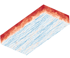
Comparisons of the instantaneous flow field between DNS and the RNL model in figure 4 show there is a visible restriction of the streamwise wavelengths. However, from the cross-stream snapshot, the realistic vortical structures are obtained, which verifies the potential of the RNL model to reflect flow structures that are important in wall turbulence (Gayme & Minnick Reference Gayme and Minnick2019). Since $N_y,N_z$ are the same as those of DNS, even though the high- and low-speed streaks are elongated and much more straight in the streamwise direction, the number and distribution of the streaky structures in the spanwise direction are accurately predicted by the RNL model. Detailed comparisons between DNS and the RNL model of other physical quantities are presented in Appendix B, such as the instantaneous normal velocity, contours of the streamwise vorticity and so on.

Figure 4. Comparison of the instantaneous streamwise velocity between DNS (a,c) and the RNL model (b,d): (a,b) $Re_{\tau }=180$ and (c,d) $Re_{\tau }=950$. The horizontal plane is at a wall distance of $y^+$ = 15.

Furthermore, the weights of the RNL-SL control model are trained through the data of RNL flow fields instead of DNS. So, it is necessary to compare the relationship between the velocity on the detection plane and the wall shear stresses in DNS and RNL flow fields. Figure 5 shows the contours of the two-point correlation coefficient $\rho$ between $v_{y^+=10}$ and $\partial u/ \partial y |_w,\partial w/ \partial y |_w$ in both DNS and the RNL model at $Re_{\tau }=180$ and $Re_{\tau }=950$. In DNS flow fields it is shown that $v_{y^+=10}$ and wall shear stresses have distinct correlation in some regions. The correlation coefficients are antisymmetric with $\partial w/ \partial y |_w$ and symmetrical with $\partial u/ \partial y |_w$ in the spanwise direction. Also, the correlation with the spanwise wall shear rate is highest at slightly downstream, which is consistent with that of Park & Choi (Reference Park and Choi2020). In RNL flow fields, distributions of the correlation coefficients are very similar to those in DNS flow fields. Limited to smaller streamwise computational grids, contours of the correlation coefficients are relatively straight in the streamwise direction. But in the spanwise direction, they share similar characteristics since the grid resolutions are the same as those of DNS. It shows that the RNL model accurately captures the relationship between the near-wall normal velocity and the wall shear stress, which makes it possible to apply machine learning control models trained by RNL data to control the real DNS field for drag reduction. Also, it is found that correlations of different Reynolds numbers are very similar in both DNS and the RNL model, indicating that machine learning control methods with similar structures are possible to be extended to high Reynolds numbers.

Figure 5. Contours of the correlation coefficients between $v_{y^+=10}$ and (a,c,e,g) $\partial u/ \partial y |_w$, (b,d,f,h) $\partial w/ \partial y |_w$. Results are shown for (a–d) DNS and (e–h) the RNL model at (a,b,e,f) $Re_{\tau }=180$ and (c,d,g,h) $Re_{\tau }=950$.

2.2. The RNL-SL control framework

Our previous study introduced the usage of CNNs for predicting wall actuations based on the streamwise or spanwise wall shear stress for drag reduction (Han & Huang Reference Han and Huang2020). As show in figure 6, the input data of CNN is wall shear stress and the output is the predicted wall blowing and suction. Based on the opposite control of Choi et al. (Reference Choi, Moin and Kim1994), the optimal wall actuations should have the same absolute value but opposite direction with the normal velocities at a detection plane. Here, the label data of CNN is opposite to the normal velocity at the detection plane, and the error between it and the output data is defined as the loss function, i.e.

(2.4)$$\begin{gather} {\rm Loss} =\frac{1}{2}\sum_{i=1}^{N} {\rm e}^{\lambda |v^i_{label}|}(v^i_{label}-v^i_{output})^2, \end{gather}$$

(2.5)$$\begin{gather}v_{label}={-}v_{y^+{=}10},v_{wall}=\sigma v_{output}, \end{gather}$$

to be minimized for updating the parameters of neural networks. In the above equations, $\lambda$ is designed for emphasizing large wall actuations and chosen as 5 in this paper; $v_{output}$ is the output of the CNN representing the predicted wall blowing and suction based on the wall shear stress. As introduced above, the amplitude of the wall blowing and suction is an important factor affecting the drag reduction rate. In the present study, considering that in a practical situation the controlled flow data are not available in advance, we train the RNL-SL control model from the uncontrolled RNL flow data. In that case, the root-mean-square (r.m.s.) value of $v_{output}$ will be larger than that of $v_{y^+=10}$ in the opposition control case, because the near-wall normal velocity is obviously decreased in the controlled flow. According to Kim & Choi (Reference Kim and Choi2017), $v_{y^+=10,rms}$ (controlled) $\approx 0.5v_{y^+=10,rms}$ (uncontrolled) under opposition control at $Re_\tau =180$. It will be difficult to compare the present control effects with those of the traditional opposition control, as the amplitudes of the wall blowing and suction are different. So, $\sigma$ in (2.5) is used to regulate the control strength at each control time step to ensure that $v_{wall,rms}$ is equal to $v_{y^+=10,rms}$ on the detection plane, i.e. $\sigma =v_{y^+=10,rms}$ (controlled) $/v_{output,rms}$, where $v_{y^+=10,rms}$ (controlled) is obtained in advance from the opposition control as a reference case.

Figure 6. Schematic of the coupled RNL and machine learning control models.

Training data of the inputs and labels are both obtained from DNS in Han & Huang (Reference Han and Huang2020). At higher Reynolds numbers, the training process of CNN will be observably elongated because a larger number of training data are required with the increasing complexity of the nonlinear relationship between the wall shear stress and normal velocities, which also causes an extra cost of obtaining training data. So it is harder and more expensive to extend it to a much more complicated flow situation with higher $Re$. The highest friction Reynolds number in Han & Huang (Reference Han and Huang2020) and Park & Choi (Reference Park and Choi2020) is 390 and 578, respectively. Furthermore, previous researches have revealed that the computational cost of neural networks is quite small compared with that of the flow solver. So, a scientific reduced-order model for calculating the flow field is necessary to accelerate the training process of the machine learning control model and extend the scope of its application to higher $Re$.

To the best of our knowledge, the RNL model has not been reported to be used for flow control problems. As seen above, the RNL model can reproduce the basic flow characteristics of turbulent channel flow to some extent with restricted streamwise Fourier components, which can easily simplify the flow representation. In this paper we apply the RNL model to drag reduction in wall turbulence coupled with machine learning technologies. The architecture of the RNL-SL control model is similar to that of the CNN control model proposed by Han & Huang (Reference Han and Huang2020). The essential difference lies in the training data of CNN. To reduce the computational cost and training difficulty, we exploit RNL simulation to obtain the training dataset including the input and label data instead of DNS. As seen in figure 6, the grids of the RNL model in the wall-normal and spanwise directions are kept the same as DNS, but the streamwise grids are limited to a few. All the training procedures are based on RNL data. When the loss function converges to the minimum, the training process of the CNN is finished, in which case the RNL-SL control model is equipped with the ability of predicting the normal velocity at the detection plane based on the wall shear stress of the RNL field. Then, it will be directly applied to the DNS flow, which is an absolutely new situation that the machine learning control model has never met. Based on the similarity of the flow field between the RNL model and DNS, the trained RNL-SL model should also be effective in controlling the realistic DNS field. We will first check its ability to predict the wall blowing and suction based on the wall shear stress and then investigate its drag reduction control effects on the real channel flow.

In the present study we also use two kinds of wall variables: streamwise and spanwise wall shear stresses, $\partial u/ \partial y |_w, \partial w/ \partial y |_w$, as the input data. Since Lee et al. (Reference Lee, Kim and Choi1998) have used a theoretical method to deduce the suboptimal control method, which obtains a concise formula describing the relationship of wall blowing and suction and spanwise wall shear stress, it is convenient to compare the control model based on RNL-SL with the analytical expression of suboptimal control method. For facilitating comparison, CNN with spanwise wall shear stress as input is constructed using a single linear convolutional layer without an activation function, and the size of the filter kernel in the streamwise direction is truncated to 1. This means that the CNN only has trainable weights in the spanwise direction. The size of the convolution kernel in the spanwise direction is determined based on previous knowledge (Lee et al. Reference Lee, Kim, Babcock and Goodman1997; Han & Huang Reference Han and Huang2020; Park & Choi Reference Park and Choi2020) that at least approximately 90 wall units are necessary for $\partial w/ \partial y |_w$ to predict the wall blowing and suction. It is noted that the performance of nonlinear CNN models is also tested with multiple convolutional layers and the hyperbolic tangent activation function. The results show that they do not significantly increase the drag reduction rate, indicating that a linear model is able to represent the relationship between $v_{y^+=10}$ and the spanwise wall shear stress.

For $\partial u/ \partial y |_w$, theoretical derivation of the suboptimal control method fails due to the oversimplification of the strong nonlinear relationship between $\partial u/ \partial y |_w$ and the normal velocities at the detection plane. We adopt a multi-layer nonlinear CNN architecture with a hyperbolic tangent activation function as the activation function. In this case, it is inevitable to involve the information of $\partial u/ \partial y |_w$ in the steamwise direction when calculating the wall blowing and suction. However, the grids in the streamwise direction are much more sparse than DNS. In order to make the CNN structure trained based on RNL data directly adapted to DNS, before training, the training data from the RNL model is interpolated in the streamwise direction to share the same grid numbers as those of DNS. The computational cost of this interpolation is negligible. Our results also verify that the style of interpolation, such as linear, polynomial interpolation or padding zero for the energy of the larger wavenumber, has little influence on the training results, so hereafter the linear interpolation is used for convenience.

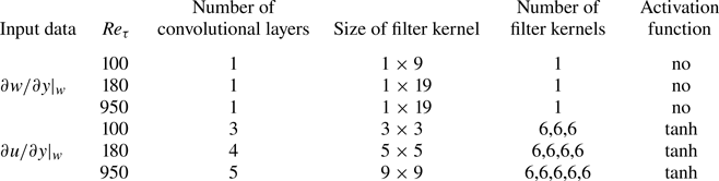
Architecture of the CNN used in the present study is shown in figure 7. Input data are the wall shear stress with the shape of $N_x \times N_z$. One convolutional layer used here includes periodic padding, convolutional operation, batch normalization and activation function. Due to the size of the filter kernel used in convolution, we use periodic padding in both the streamwise and spanwise directions to avoid the loss of edge information. We use the hyperbolic tangent activation function instead of rectified linear units (ReLU) that is commonly used in CNN (Nair & Hinton Reference Nair and Hinton2010), in order to retain negative neural input and output in the training process. The corresponding hyperparameters of the CNN architecture are summarized in table 2, which are chosen based on our previous attempts based on DNS data (Han & Huang Reference Han and Huang2020).

Figure 7. Architecture of the CNN used in the present study. Here $(2m+1)\times (2n+1)$ is the size of filter kernel and $N_{fi}$ represents the number of filter kernels used in the $i$th convolutional layer. The output dimensions of each layer are shown below them. The widths of periodic padding in the streamwise and spanwise directions ($m,n$) are determined by the shape of the filter kernel to ensure that the output dimensions after convolution remain consistent with the input.

Table 2. Details of the CNN architectures for different cases.

2.3. The RNL-RL control framework

Even though prediction of the optimal wall blowing and suction by the RNL-SL model only requires the input of wall shear stress, its training process is dependent on the velocity within the flow field. In this section we combine the RNL model with RL, which undergoes training without reliance on labelled data. Due to the computational efficiency of the RNL model, we will further explore the potential of applying the RNL-RL control model to turbulent channel flows at higher Reynolds numbers.

As shown in figure 6, comparing with the RNL-SL model, it is seen that with the help of the RL architecture that updates the network parameters based on the reward of applying the RL output (action) to control the flow instead of the error between output and the label data, the RNL-RL model eliminates the dependence of information on the detection plane. The RL depends on a well-designed reward for better exploration of the unknown output region to optimize the weights of its neurons. The training datasets of the RL model, including the input data (state), the output data (action) and the reward of applying this action to control the turbulent channel flow, are acquired after each interaction between the RL control and the flow field. So, each interaction needs a numerical simulation of several time steps. Due to the lack of label data to guide the training, the RL model needs to observe the flow environment and adjust its action repeatedly within several epochs in order to obtain a larger reward. When one epoch finishes, the flow environment will be reset and the next epoch of training begins. In each epoch with a time period of $T$, the RL agent described by CNN gets the state ($s_t$, defined as the wall shear stress) from the initial environment as input data, which is an instantaneous field of fully developed turbulent channel flow. After the operation of CNN, the RL agent outputs the action ($a_t$), which is thought to be the optimal wall blowing and suction based on the present CNN parameters. Then, the controlled RNL channel flow by $a_t$ is advanced within a state step, which contains 50 simulation time steps according to Lee et al. (Reference Lee, Kim and Lee2023). Then the next state ($s_{t+1}$) is reached. In the present study, one epoch of RL $T$ involves 800, 1200 and 2000 state steps at $Re_{\tau }=100,180,950$, respectively. The reward of a state step is defined as

(2.6)\begin{equation} r_t=\frac{\overline{\tau_0}-\overline{\tau_w}}{\overline{\tau_0}}, \end{equation}

where $\overline {\tau _w}$ and $\overline {\tau _0}$ denote the averaged frictions with and without control within a state step, respectively. The training set ($s_t,a_t,r_t,s_{t+1}$) of one state step is then recorded into a replay buffer, whose memory size is chosen as 30 000, and when the replay buffer is full, the oldest data will be removed. During the training process, a group of training sets is chosen randomly from the replay buffer to decrease the correlation between them over time. The batch size is set to 64, which is determined based on previous knowledge.

The RL model used in the present study is trained by the deep deterministic policy gradient (DDPG) algorithm (Lillicrap et al. Reference Lillicrap, Hunt, Pritzel, Heess, Erez, Tassa, Silver and Wierstra2015), which is especially useful in continuous action problems. The DDPG consists of two networks: the actor network ($\mu _{\theta ^{\mu }}$) and the critic network ($Q_{\theta ^{Q}}$). The actor network is responsible for generating the output action based on the observed state, as mentioned earlier. Specifically, the output action is obtained using the equation $a_t=\mu _{\theta ^ {\mu }} (s_t)$. On the other hand, the critic network aims to evaluate the action by fitting a value function $Q_{\theta ^{Q}} (s_t,a_t)$. This value function represents the expected return after taking the action $a_t$ in the state $s_t$, i.e.

(2.7)\begin{equation} Q_{\theta^{Q}} (s_t,a_t) = \mathbb{E} \left[\sum_{i=t}^{T} \gamma^{i-t} r(s_i,a_i)\right],\end{equation}

where $\mathbb {E}$ means the expectation and $\gamma$ is the time discount rate indicating the decaying effect of the action over time until the end of the epoch, which is chosen as 0.99 according to Fan et al. (Reference Fan, Yang, Wang, Triantafyllou and Karniadakis2020b), Paris, Beneddine & Dandois (Reference Paris, Beneddine and Dandois2021). Here $\theta ^{\mu }$ and $\theta ^{Q}$ are the parameters of actor and critic networks; $\theta ^{\mu }$ is optimized by maximizing the expected total reward $Q_{\theta ^{Q}}$ and $\theta ^{Q}$ is updated based on the temporal difference error defined as the difference between the estimated value function of the current state-action pair and the value function of the next state-action pair. More details can be found in Appendix D.

The CNN architecture and its corresponding hyperparameters used in the actor network are the same as discussed in figure 7 and table 2, since their input and output are the same. The key to successful training of RL is based on a better estimate of the value function interpreted by the critic network. Referring to Lee et al. (Reference Lee, Kim and Lee2023), we use a relatively complex network as shown in figure 8. Different from the actor network based on figure 7, input of the critic network includes both the state and its corresponding action calculated from the actor network. The output of the critic network is the value of $Q_{\theta ^{Q}}$, which is utilized to assess the desirability of the action in the current state. Here, zero padding is used before each convolutional layer for simplicity. Due to substantial dimension reduction from input to output, average pooling is incorporated into certain convolutional layers and a fully connected layer is added before the output. The hyperparameters of the critic network are given in table 3.

Figure 8. Architecture of the critic network used in DDPG. The output dimensions of each layer are shown below them. Conv 1 and Conv 2 represent two kinds of convolutional layers. Conv 2 has an additional average pooling layer compared with Conv 1.

Table 3. Hyperparameters used in the critic networks for different cases. Here, numbers of the filter kernels in each convolutional layer are all fixed as 32. The order Conv 1 + Conv 2 + (Conv 1) $\times$ 3 is used at $Re_{\tau }=100$. The order (Conv 1 + Conv 2) $\times$ 2 + Conv 1 is used at $Re_{\tau }=180,950$. It is noted that these hyperparameters remain the same for both $\partial w/ \partial y |_w$ and $\partial u/ \partial y |_w$.

3.1. Training process

There are three kinds of variables of RNL data: streamwise mean, fluctuation and their summation, based on which, the RNL-SL model can be trained separately when using $\partial w/ \partial y |_w$ as input. For $\partial u/ \partial y |_w$, given the demand of streamwise information of physical quantities, streamwise mean variables cannot be used for training. Since their training processes are almost the same, we only show the results based on the total (summation) quantities of RNL data. The training dataset consists of 2000 instantaneous RNL fields including the instantaneous wall shear stress and the corresponding normal velocities on the detection plane at $y^+=10$. The amount of training data is sufficient thanks to the characteristics of weight sharing of CNN architecture, because the output at each grid point of a convolutional layer is calculated using the same filter kernal for convolution operation. Figure 9 shows the averaged loss and correlation coefficient between the output and label data over each training epoch. It is obvious that all the losses decrease rapidly with epoch and eventually achieve a convergent value. Variations of the correlation coefficients exhibit the same variation tendency. All the correlation coefficients are around 0.90, indicating great interpretation of the relationship between wall shear stresses and the normal velocity on the detection plane by the RNL-SL model. It also shows that the number of training epochs of $\partial u/ \partial y |_w$ is almost 10 times larger than that of $\partial w/ \partial y |_w$ because of the complexity of their CNN architectures. The fluctuations of the loss and correlation coefficient of $\partial u/ \partial y |_w$ are much larger, implying the complex nonlinear relations between the input and output of CNN, making it difficult for training. However, when comparing the training processes of $Re_{\tau }=180$ with that of $Re_{\tau }=950$, it is found that the necessary epochs do not increase distinctly with Reynolds number for both $\partial w/ \partial y |_w$ and $\partial u/ \partial y |_w$.

Figure 9. Training loss (black lines) and correlation coefficient (red dashed lines) between the output and label of the RNL-SL model in terms of epoch based on the input of (a–c) $\partial w/ \partial y |_w$ and (d–f) $\partial u/ \partial y |_w$: (a,d) $Re_{\tau }=100$, (b,e) $Re_{\tau }=180$, (c,f) $Re_{\tau }=950$.

Due to the simple architecture of CNN for $\partial w/ \partial y |_w$, we can easily draw out the distribution of the filter kernels in the spanwise direction in figure 10. We compare the models trained with three different kinds of RNL data as mentioned above as well as the weights obtained based on DNS data from Han & Huang (Reference Han and Huang2020), which have been proved perfectly consistent with the theoretical solution of suboptimal control. It is surprising that the weight distributions of all the cases are analogous with each other. Weights near the point of interest have the largest value and then decay rapidly to almost zero at the boundary of the sensing region of the filter kernel. It is worth noting that the weight distributions do not demonstrate strict antisymmetry as observed in the analytical solutions of the suboptimal control, even though we attempted to triple the size of the training data. But it has only a small influence on the drag reduction effect, indicating that the training data are sufficient and the training process is converged. The results of $Re_{\tau }=950$ have not been shown in previous studies, but the similar distribution profile and good prediction performance shown below verifies their credibility. Successful training of the CNN model based on RNL data reveals that the RNL simulation makes a reliable prediction of the turbulent channel flow, especially in the near-wall region.

Figure 10. Weight distribution in the spanwise direction of the RNL-SL model based on $\partial w/ \partial y |_w$ from (a) $Re_{\tau }=100$, (b) $Re_{\tau }=180$, (c) $Re_{\tau }=950$. The model is trained based on the total velocity ($\boldsymbol {u}$), fluctuation velocity ($\boldsymbol {u}^{'}$) and mean velocity ($\boldsymbol {U}$) from the RNL model and compared with that from DNS.

3.2. Comparison of prediction performance in the RNL model and DNS

To illustrate the prediction performance of the trained RNL-SL models, we apply them to both RNL and DNS flow fields, which are new for them to test. The time histories of the correlation coefficients at the steady stage in the RNL model and DNS are shown in figure 11. For $\partial w/ \partial y |_w$, the predicted correlation coefficients of the RNL model at different Reynolds numbers almost remain constant without decaying with time. Their averaged values are all around 0.9, which are nearly the same as those of the training process. It indicates that the RNL-SL model is well trained and can effectively reflect the relationship between wall shear stress and the predicted wall blowing and suction. When directly applying the RNL-SL model to the DNS flow field, the correlation coefficients obtained are a little smaller than those in the RNL test flow field. However, the averaged values are still over 0.8, which is larger than that using other machine learning methods, e.g. the Lasso (Tibshirani Reference Tibshirani1996), random forest (Breiman Reference Breiman2001) and fully connected neural networks as discussed in Park & Choi (Reference Park and Choi2020). For $\partial u/ \partial y |_w$, it is observed that there appears to be a more distinct oscillation of the correlation coefficient than that in the training process. However, the averaged values of the RNL flow field are almost kept at a similar level close to the training cases, which are about 0.9, 0.8 and 0.8 at $Re_{\tau }=100,180,950$, respectively. The correlation coefficients in the DNS test field decline sharply to 0.6, 0.4 and 0.38 as compared with those in the RNL field. Differences of the prediction performance in the RNL model and DNS for $\partial u/ \partial y |_w$ can be attributed to deficiency of the flow field details in the streamwise direction, which is necessary for predicting the normal velocities from $\partial u/ \partial y |_w$. Nevertheless, these coefficients are stable without changing with time.

Figure 11. Test results of the correlation coefficient between the output and the label of the RNL-SL model in terms of time based on the input of (a–c) $\partial w/ \partial y |_w$ and (d–f) $\partial u/ \partial y |_w$: (a,d) from $Re_{\tau }=100$, (b,e) from $Re_{\tau }=180$, (c,f) from $Re_{\tau }=950$. Results are compared between DNS and the RNL model by using the same model trained by RNL data.

Figures 12–14 show the instantaneous prediction results based on the RNL-SL models in both the RNL and DNS flow fields at different Reynolds numbers. Due to the restriction of the streamwise modes in the RNL model, the contours of the normal velocities at $y^+=10$ show elongated features (figures 12–14a), which can also be seen in the prediction results (figures 12–14b,c). It is also seen that the performances of $\partial w/ \partial y |_w$ always outperform those of $\partial u/ \partial y |_w$, consistent with the correlation coefficients in figure 11. Figures 12–14(e,f) are obtained directly by using the corresponding RNL-SL model in the DNS flow field. Despite the substantial differences between the labels from the RNL model and DNS (comparing figures 12–14(a) with (c)), the RNL-SL models are also effective for prediction. It is not difficult to infer that the control model trained only based on RNL data can give a good prediction of the velocity field in the spanwise direction, because the RNL model and DNS have the same spanwise computational domain and grid resolution. On the other hand, the prediction performance based on $\partial w/ \partial y |_w$ is much better than that of $\partial u/ \partial y |_w$. It is not only because of the simple relationship between $\partial w/ \partial y |_w$ and $v$ at $y^+=10$, but also because the CNN model based on $\partial w/ \partial y |_w$ does not need the streamwise direction information and the model based on $\partial u/ \partial y |_w$ is influenced by information in the streamwise direction, especially when using a larger number of convolution layers. According to table 1, in order to reduce the computational cost, fewer grids in the streamwise direction are used and the ratio of $N_z$ to $N_x$ becomes larger with Reynolds numbers. When training the RNL-SL model at a larger Reynolds number, the deficiency of the flow simulation in the streamwise direction becomes more evident. Lack of some effective and key information makes it perform not so well as that using the spanwise wall shear stress. However, the flow features in the spanwise direction, such as the alternating positive and low-speed streaky structures are evident and similar to the label data.

Figure 12. Instantaneous contours of $v_{label}$ and $v_{wall}$ at $Re_{\tau }=100$: (a,d) $v_{label}$, (b,e) $v_{wall}$ based on $\partial w/ \partial y |_w$, (c,f) $v_{wall}$ based on $\partial u/ \partial y |_w$. Plots (a–c) are from the RNL model and (d–f) are from DNS.

Figure 13. Instantaneous contours of $v_{label}$ and $v_{wall}$ at $Re_{\tau }=180$: (a,d) $v_{label}$, (b,e) $v_{wall}$ based on $\partial w/ \partial y |_w$, (c,f) $v_{wall}$ based on $\partial u/ \partial y |_w$. Plots (a–c) are from the RNL model and (d–f) are from DNS.

Figure 14. Instantaneous contours of $v_{label}$ and $v_{wall}$ at $Re_{\tau }=950$: (a,d) $v_{label}$, (b,e) $v_{wall}$ based on $\partial w/ \partial y |_w$, (c,f) $v_{wall}$ based on $\partial u/ \partial y |_w$. Plots (a–c) are from the RNL model and (d–f) are from DNS.

3.3. Application to active control

In this subsection we apply the well-trained RNL-SL models by the uncontrolled RNL data to DNS flow fields for drag reduction in a turbulent channel flow at different Reynolds numbers. Table 4 shows the averaged correlation coefficients between the predicted wall blowing and suction and the normal velocities at the detection plane in the controlled DNS flow. Comparing these results with those shown in figure 11, it can be concluded that based on $\partial w/ \partial y |_w$, the trained RNL-SL models perform well for prediction in both the uncontrolled and controlled flow fields, and their correlation coefficients are almost the same. Based on $\partial u/ \partial y |_w$, the averaged correlation coefficients decrease as compared with that based on the uncontrolled flow data, indicating the influence of the wall blowing and suction on the relationship between streamwise wall shear stress and the normal velocities at $y^+=10$. This phenomenon was also detected by Park & Choi (Reference Park and Choi2020), where the correlation coefficient is decreased more than that of the present study. The reason may be that they use a more complex CNN architecture for training. In the present study, since the streamwise modes of the RNL training data are substantially restricted, using a CNN model with more convolutional layers and filter kernels does not improve the training and prediction accuracies obviously. Even though the prediction performance in the controlled flow field is a little lower than that of the uncontrolled one, the predicted wall blowing and suction also maintain approximately linear relations with the labels as shown in figure 15 taken the cases of $Re_{\tau }=180$, for example. The predicted wall blowing and suction can also reproduce the main flow characteristics of the flow field, as shown by the instantaneous contours in figure 16. The results are consistent with those in figures 12–14(d–f), where the RNL-SL models with input of $\partial w/ \partial y |_w$ make a better prediction of not only the correlation coefficient of the whole flow field but also the details of the flow structures. When using $\partial u/ \partial y |_w$ as input, the RNL-models’ prediction capacity decreases and the predicted velocity distribution appears with nonconformity from the view within some small windows of the flow field, which explains the reason of lower drag reduction rates shown below.

Table 4. Averaged correlation coefficients between the output of the RNL-SL model and the normal velocities at $y^+=10$ of the controlled DNS flow based on the streamwise and spanwise wall shear stresses at $Re_{\tau }=100,180,950$.

Figure 15. Scatter plots of $v_{label}$ and $v_{wall}$ at $Re_{\tau }=180$ based on (a) $\partial w/ \partial y |_w$ and (b) $\partial u/ \partial y |_w$.

Figure 17 presents the time histories of the wall shear stress of controlled flow based on $\partial w/ \partial y |_w$ and $\partial u/ \partial y |_w$ compared with the uncontrolled ones at different Reynolds numbers. The wall shear stress ($\tau _w$) of the controlled case is normalized by the uncontrolled case ($\tau _0$) at each Reynolds number. It is obvious that all the cases controlled by RNL-SL models obtain drag reduction and when the control begins at $t=0$, the wall shear stress decreases immediately and reaches a new level with a lower skin friction. The time interval to reach this new level becomes shorter with the increase of Reynolds number. The drag reduction rate is defined as

(3.1)\begin{equation} DR=\frac{\tau_0 - \tau_w}{\tau_0}=1-\frac{\tau_w}{\tau_0} , \end{equation}

which is larger based on $\partial w/ \partial y |_w$ than that of $\partial u/ \partial y |_w$. This is consistent with the prediction performance as listed in table 4. Furthermore, to compare the drag reduction rates based on the RNL-SL model with those of the traditional opposition control, drag reduction rates of different cases are given in table 5. For the opposition control based on the normal velocities at $y^+=10$ of $Re_{\tau }=180$, 20 % drag reduction is obtained, which is the same as those obtained in the previous studies (Chang et al. Reference Chang, Collis and Ramakrishnan2002; Chung & Talha Reference Chung and Talha2011). So far few researches have reported the opposition control results for $Re_{\tau }=950$; $DR=18\,\%$ in the present study is close to the value of 16 % reported by Deng et al. (Reference Deng, Huang and Xu2016) for $Re_{\tau }=1000$ at $y^+ \approx 9.8$ using a spectral DNS solver. Drag reduction rates of the RNL-SL models based on $\partial w/\partial y |_w$ can almost reach over 95 % of those based on the opposition control, which means that the wall blowing and suction predicted by $\partial w/ \partial y |_w$ capture well the main characteristics of the optimal velocities on the detection plane. By means of the simplicity and computation economy of the RNL training data, the coupled RNL and CNN method can be easily applied to higher Reynolds numbers. Limited to the prediction performances of the RNL-SL models based on $\partial u/ \partial y |_w$, drag reduction rates are always lower than that based on $\partial w/ \partial y |_w$ at all the Reynolds numbers. But the drag reduction rates based on $\partial u/\partial y |_w$ are all over 12 % at different Reynolds numbers up to $Re_{\tau }=950$, which is still larger than those reported in the previous studies, e.g. 10 % from a two-dimensional linear controller at $Re_{\tau }=100$ (Lee et al. Reference Lee, Cortelezzi, Kim and Speyer2001), 12 % from a control scheme optimized by a genetic algorithm at $Re_{\tau }=100$ (Morimoto et al. Reference Morimoto, Iwamoto, Suzuki and Kasagi2002), 11.5 % from an improved suboptimal control at $Re_{\tau }=180$ (Fukagata & Kasagi Reference Fukagata and Kasagi2004) and 11 % from a multiple input and output CNN controller at $Re_{\tau }=180$ (Park & Choi Reference Park and Choi2020).

Figure 16. Instantaneous contours of $v_{label}$ and $v_{wall}$ from the controlled DNS flow field: (a,d,g) $v_{label}$, (b,e,h) $v_{wall}$ based on $\partial w/ \partial y |_w$, (c,f,i) $v_{wall}$ based on $\partial u/ \partial y |_w$. Plots (a–c) are from $Re_{\tau }=100$, (d–f) are from $Re_{\tau }=180$ and (g–i) are from $Re_{\tau }=950$. The correlation coefficients of $Re_{\tau }=100,180,390$ are 0.91, 0.88, 0.81 based on $\partial w/ \partial y |_w$ and 0.52, 0.39, 0.36 based on $\partial u/ \partial y |_w$, respectively.

Figure 17. Time histories of the streamwise wall shear stress of uncontrolled and controlled flows based on $\partial w/ \partial y |_w$ and $\partial u/ \partial y |_w$: (a) $Re_{\tau }=100$, (b) $Re_{\tau }=180$ and (c) $Re_{\tau }=950$.

Table 5. Drag reduction rates (DR) from different cases of the RNL-SL model control and corresponding opposition control.

Figure 18 presents the profiles of the velocity fluctuations of the controlled channel flow and the uncontrolled one at different Reynolds numbers. All the components of the velocity fluctuations were substantially suppressed by the wall blowing and suction of the RNL-SL models, among which the suppression on the wall-normal velocity from the controller based on $\partial w/ \partial y |_w$ is the most pronounced. Focusing on $v_{rms}$, it can be found that it has a value greater than 0 at the wall and is almost equal with that of $y^+=10$, which determines a similar control strength with that of the opposition method according to (2.5). The value $v_{rms}$ decreases firstly and then increases with $y^+$. It forms a minimum value close to zero between the wall and $y^+=10$, where a ‘virtual wall’ is established to prevent the momentum and energy transfer, resulting in drag reduction (Hammond et al. Reference Hammond, Bewley and Moin1998). Figure 19 shows the instantaneous vortical structures identified by using the second invariant of the velocity gradient tensor ($Q$). With the same value of $Q$, the controlled flow fields show fewer vortices compared with the uncontrolled cases, which verifies that the wall blowing and suction destroy the vortical structures. Furthermore, the degree of the weakening of the vortex is proportional to the drag reduction rate, which is consistent with the results shown in table 5.

Figure 18. Profiles of the turbulent velocity fluctuations, $u_{rms}$ (line with square), $v_{rms}$ (solid line) and $w_{rms}$ (dashed line) from cases of no control (black), controlled based on $\partial w/ \partial y |_w$ (red) and $\partial u/ \partial y |_w$ (blue): (a) $Re_{\tau }=100$, (b) $Re_{\tau }=180$, (c) $Re_{\tau }=950$.

Figure 19. Instantaneous vortical structures identified by the isosurface of $Q$ within the lower half-channel flow for uncontrolled cases (a,d,g), controlled cases based on $\partial w/ \partial y |_w$ (b,e,h) and $\partial u/ \partial y |_w$ (c,f,i). The vortical structures are coloured by the normal velocities. Results are shown for (a–c) $Re_{\tau }=100$, $Q=0.1$; (d–f) $Re_{\tau }=180$, $Q=1$; (g–i) $Re_{\tau }=950$, $Q=30$.

4.1. Training process

As described in § 2.3, RNL-RL discovers the optimal control strategy through iterative interactions with the flow field within a single epoch. When an epoch ends, the environment will be reset to the uncontrolled one and a new iteration of learning begins. Figure 20 shows the training process of the RNL-RL model based on the input of $\partial w/ \partial y |_w$. The averaged reward within the second half-epoch increases rapidly with each epoch and is converged to a constant, indicating that the model has been well trained. The minimum number of training epochs is about 10 for all the cases at $Re_{\tau }=100,180,950$. It is similar to that of 16 epochs trained through the DNS flow field at $Re_{\tau }=180$, as reported by Lee et al. (Reference Lee, Kim and Lee2023). Due to the usage of the RNL model for training, the computational cost is over 10 times lower at the same Reynolds number of $Re_{\tau }=180$. At $Re_{\tau }=950$, the computational cost has fallen even more sharply (by over 30 times as shown in table 1) due to the fewer grids used in the streamwise direction, where $N_x=16$ in the RNL model and $N_x=512$ in DNS, for example. So, the present RNL-RL model can be easily extended to control the turbulent flow at a much higher Reynolds number. During the training process, we also monitor the correlation coefficient between the output of the RNL-RL model and the normal velocities on the detection plane. Figure 20(d,e,f) clearly shows that during the last five epochs of the training process of the RNL-RL model, the correlation coefficient at each state step remains around 0.8, which is similar to that of the test results of the RNL-SL model shown in figure 11. This result shows that the control strategy learned by RL based on $\partial w/ \partial y |_w$ without label data also leads to a similar result with the opposition control method.

Figure 20. Reward (a–c) and the correlation coefficient (d–f) between the output of the RNL-RL model and the normal velocities at $y^+=10$ in terms of epoch based on the input of $\partial w/ \partial y |_w$: (a,d) $Re_{\tau }=100$, (b,e) $Re_{\tau }=180$, (c,f) $Re_{\tau }=950$.

To learn more details about the training process, figure 21(a) shows the normalized wall shear stress of uncontrolled flow and the controlled flow by the RNL-RL model within the first 10 epochs. It can be found that at the beginning of training, the RNL-RL model fails to output effective wall blowing and suction, resulting in the increase of wall shear stress. However, the RNL-RL model continuously adjusts its control strategy within the following epochs and succeeds in reducing the friction at the wall. Also, the drag reduction rate increases with each epoch, showing better control performance. The corresponding correlation coefficient also appears to have a similar variation trend in figure 21(b).

Figure 21. Wall shear stresses of the uncontrolled and controlled flows by the RNL-RL model (a) and the corresponding correlation coefficient between the output of the RNL-RL model and the normal velocity at $y^+=10$ (b) within the first 10 epochs at $Re_{\tau }=180$.

Figure 22 compares the converged weight distribution of the RNL-RL model with that of the RNL-SL model. It is surprising that results agree well with each other, which means that the CNN, which describes the relation between $\partial w/ \partial y |_w$ and the optimal wall blowing and suction determined by RNL-SL and RNL-RL models, shares the same weight distribution. In other words, the control strategy discovered from our RNL-RL model that only uses spanwise wall shear stress in RNL flow fields as input, is close to the globally optimal solution.

Figure 22. Weight distribution in the spanwise direction of the RNL-RL model based on $\partial w/ \partial y |_w$ at (a) $Re_{\tau }=100$, (b) $Re_{\tau }=180$ and (c) $Re_{\tau }=950$. The model is trained based on the total velocity ($\boldsymbol {u}$) and compared with the RNL-SL model.

4.2. Application to active control

Even though the training process in RNL flow fields shows effective drag reduction, it still needs to test whether the RNL-RL model also works well in real DNS flow fields. Figure 23 shows the drag reduction results in a DNS test. It is notable that the drag reduction rate is larger than the convergent reward shown in figure 20. The reason is that during the period of each epoch, as shown in figure 21(a), the wall shear stress has not reached the steady stage. But it has no influence on the training of the RNL-RL model, because in this period of epoch, the model has been trained well enough and increasing the period will not improve the training effect. It has also been discussed in detail in Han et al. (Reference Han, Huang and Xu2022) about the influence of $T$ on the training results. Moreover, it is found that the drag reduction rates at different Reynolds numbers are almost the same as those of the RNL-SL models. According to table 5, drag reduction rates of our RNL-RL models also achieve 90 %, 95 % and 89 % of those with opposition control.

Figure 23. Comparison of time histories of the streamwise wall shear stress of uncontrolled and controlled flows based on $\partial w/ \partial y |_w$ from the RNL-SL and RNL-RL models: (a) $Re=100$, (b) $Re=180$, (c) $Re=950$.

Furthermore, the control mechanism determined by RNL-RL is analysed and compared with that of the opposition control. The previous researches have shown that the spanwise wall shear stress is an indicator of the streamwise vortices, better than wall pressure and streamwise wall shear stress, because $\partial w/ \partial y |_w$ is the spanwise trace left by the streamwise vortices on the wall and they show strong correlation in the near-wall region (Kravchenko et al. Reference Kravchenko, Choi and Moin1993; Ge, Xu & Cui Reference Ge, Xu and Cui2011). Ge et al. (Reference Ge, Xu and Cui2011) further compared the differences of the cross-correlation coefficients between $\partial w/ \partial y |_w$ and $\omega _x$ from the uncontrolled flow field and the controlled one by random wall blowing and suction. It was found that they almost remained the same as each other, which meant that the correlation between $\partial w/ \partial y |_w$ and $\omega _x$ was robust and would not be affected by the wall actuations. In that case, by using $\partial w/ \partial y |_w$ as the input, our RNL-RL model should also be able to detect the appearance of the streamwise vortices and determine wall blowing and suction for control.

To clarify this control mechanism, referring to Lee et al. (Reference Lee, Kim and Lee2023), we show the instantaneous contours of the streamwise vorticity and the wall blowing and suction in figure 24. From the most prominent blue region in figure 24(a) (representing a negative streamwise vorticity), it is seen that sweep and ejection events are induced on the left and right sides, respectively. Within this region, the control strategy derived by RL involves applying blowing in the sweeping region and suction in the ejection region. This control strategy is similar with the opposition control and the suboptimal control based on $\partial w/ \partial y |_w$, since both of them aim at suppressing the up-and-down motion induced by the streamwise vortices (Choi et al. Reference Choi, Moin and Kim1994; Lee et al. Reference Lee, Kim and Choi1998,  Reference Lee, Kim and Lee2023). The most prominent red region shown in figure 24(b) also exhibits a consistent drag reduction mechanism. Also, the effect of wall blowing and suction by the RNL-RL model on the near-wall turbulence is shown by the two-point correlation between the spanwise wall shear stress and streamwise vorticity in figure 25. It is found that these correlations are suppressed by the RNL-RL control and the position of the correlation minima appears further away from the wall, indicating the weakening of the streamwise vortices. So, it can be concluded that if only using $\partial w/ \partial y |_w$ as input, RNL-RL tends to capture the streamwise vortices suppression mechanism as its optimal solution, which has also been reported by Lee et al. (Reference Lee, Kim and Lee2023).

Figure 24. Instantaneous contours of the streamwise vorticity with $v$–$w$ velocity vector field and the wall blowing and suction based on the RNL-RL model at $Re_\tau =180$ at different times of (a,b). Lines of the $z$ gradient of the spanwise wall shear stress ($(\partial / \partial z)/ \partial w / \partial y |_w$) and the wall blowing and suction are compared. Here the asterisk represents normalization by the r.m.s. values of themselves.

Figure 25. Contours of the two-point correlation between the spanwise wall shear stress and the streamwise vorticity in (a) uncontrolled and (b) controlled flow by the RNL-RL model at $Re_\tau =180$.

Different with the present work, Sonoda et al. (Reference Sonoda, Liu, Itoh and Hasegawa2023), Guastoni et al. (Reference Guastoni, Rabault, Schlatter, Azizpour and Vinuesa2023) applied RL to determine the optimal wall blowing and suction with the input of streamwise and normal velocity fluctuations on the detection plane at $y^+=15$. Moreover, they used a deep neural network to represent the RL agent. It can be viewed as a point-to-point style, as dictated in (1) of Guastoni et al. (Reference Guastoni, Rabault, Schlatter, Azizpour and Vinuesa2023) and (3.4) and (3.5) of Sonoda et al. (Reference Sonoda, Liu, Itoh and Hasegawa2023). The wall blowing and suction at one grid point is only dependent on the streamwise and normal velocities at the same position on the detection plane. On the other hand, since CNN is used as the RL agent in the present study, the wall blowing and suction at a grid point is determined by the wall shear stresses within a certain range around it. So, their control strategy indicates an abrupt switch between strong wall blowing and suction for downwelling of high-speed fluids and upwelling of low-speed fluids. Also, due to the dependence on the streamwise velocity fluctuation on the detection plane, the control strategy of Guastoni et al. (Reference Guastoni, Rabault, Schlatter, Azizpour and Vinuesa2023) shows an inclination angle of the boundary between wall blowing and suction. But our RNL-RL model is almost independent of the streamwise velocity fluctuation, similar with that of opposition control, as shown in figure 26(b). The wall blowing and suction explored from our RNL-RL model extends longitudinally in the streamwise direction and alternatively changes along the spanwise direction reflecting instantaneous near-wall streaky structures (figure 26a), whereas the wall actuations from their model are uniform in the spanwise direction and the streamwise wavelength is equal to the streamwise domain size. Besides the differences from the input data and the RL architecture, different hyperparameters used for training will also lead to different local optimum solutions (Lee et al. Reference Lee, Kim and Lee2023).

Figure 26. Contours of the instantaneous wall blowing and suction by the RNL-RL model in (a) the $x$–$z$ plane and (b) the $u'$–$v'$ plane at $Re_\tau =180$. Here $u'$ and $v'$ of (b) are from $y^+=10$. The wall blowing and suction velocities corresponding to the unsampled $u'$ and $v'$ are obtained through linear interpolation.

Furthermore, we also carry out RNL-RL training based on the input of $\partial u/ \partial y |_w$; but it does not produce effective drag reduction results, even though the training process is convergent and appears to have drag reduction effects in the RNL field. When applying the trained model to control the DNS flow, the output wall blowing and suction do not produce effective drag reduction. It may be due to the different flow fields in the streamwise direction between the RNL model and DNS for training based on $\partial u/ \partial y |_w$. For the SL of CNN discussed in the above sections, even though there are also losses of the information in the streamwise direction, the output of the RNL-SL model can still give acceptable prediction with the guidance of label data. But for the RNL-RL model, the adjustment of the action is completely dependent on the value function adopted by the RL agent based on its observation of the flow environment. In this case, the restriction in the streamwise direction makes the RNL-RL model trained by RNL data not applicable in control of the DNS flow field. This needs to be further investigated in the future. As for a preliminary attempt of combining the RNL model with RL, successful application based on the spanwise wall shear stress to the turbulent channel flow at up to $Re_{\tau }=950$ provides us an enlightening insight that a physical reduced-order model can overcome the difficulty of high computational cost in the RL training and improve the feasibility of applying a machine learning control method to practical situations.