


1. Introduction
Evaporation is a ubiquitous phenomenon in nature and has many practical applications, such as evaporative cooling, material coating and disease diagnosis (Pinto et al. Reference Pinto, Silva, Porteiro, Míguez and Baptista2018; Yang, Cui & Lan Reference Yang, Cui and Lan2019; Brutin et al. Reference Brutin, Sobac, Loquet and Sampol2011). With the emergence of nanotechnologies, these applications have now ventured into the realm of the nanoscale. One example is evaporative distillation using nanoporous membranes with pore diameters of the order of nanometres  $({\sim }100\ {\rm nm})$, which allows unprecedented efficiency in the separation of substances (Khayet Reference Khayet2011; Dong et al. Reference Dong, Poredoš, Ma and Wang2022). In addition, nanoscale evaporation processes are being exploited in electronic components to enable highly efficient heat dissipation (Khodabandeh & Furberg Reference Khodabandeh and Furberg2010; Vaartstra et al. Reference Vaartstra, Zhang, Lu, Díaz-Marín, Grossman and Wang2020). It is clear, therefore, that computational tools capable of accurately simulating nanoscale evaporative flow are paramount to the effective design and operation of these nanoscale devices. The accurate modelling of nanoscale evaporation processes poses, however, significant physical challenges due to the involvement of distinct spatial domains spanning multiple lengths and time scales.
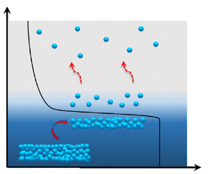
As depicted in figure 1, four regions can typically be distinguished in the flow field of an evaporating liquid: the liquid bulk, the interface, the Knudsen layer (which marks the initial region of the vapour phase) and the vapour bulk (Frezzotti Reference Frezzotti2011; Frezzotti & Barbante Reference Frezzotti and Barbante2017; Aursand & Ytrehus Reference Aursand and Ytrehus2019). The interface (with a size of the order of a molecular diameter) and the Knudsen layer (with a size of the order of the mean free path) connect the liquid and vapour bulk regions. In these transitional layers, the fluid is in a non-equilibrium state, and the macroscopic variables are subject to substantial variations, which manifest themselves as ‘jumps’ on the macroscopic scale. Accurately representing the exchange of mass, momentum and energy between the vapour and the liquid bulk is a key problem in properly accounting for evaporation.

Figure 1. In evaporation, a bulk liquid region and a bulk vapour region are separated by a molecular scale interface. Adjacent to the interface on the vapour side is the non-equilibrium region Knudsen layer of the order of the mean free path. Across the interface and Knudsen layer, macroscopic quantities such as density  $n$, velocity
  $u$, and temperature
  $T$ undergo sharp transitions that appear discontinuous on the macroscale.
The vapour within the Knudsen layer is rarefied, and so extensive studies have been undertaken to investigate the flow dynamics within this region using classical gas kinetic theory (Ytrehus Reference Ytrehus1997; Frezzotti & Barbante Reference Frezzotti and Barbante2017). Approximately 140 years ago, Hertz and Knudsen formulated an expression for the evaporation mass flux in this region, known as the Hertz–Knudsen (H–K) formula (Hertz Reference Hertz1882; Knudsen Reference Knudsen1915). While the H–K formula can capture some aspects of the evaporation process, its inability to account for the downstream vapour velocity hinders its accuracy in predicting flow properties (Persad & Ward Reference Persad and Ward2016; Aursand & Ytrehus Reference Aursand and Ytrehus2019). The H–K formula was later improved by Schrage (Reference Schrage1953). While this modified equation is still widely used, it has shortcomings, such as inapplicability beyond weak evaporation conditions (Vaartstra et al. Reference Vaartstra, Lu, Lienhard and Wang2022). This gap in knowledge has been filled by subsequent contributions that incorporate the conservation of mass, momentum and energy. For evaporation from a planar liquid surface, the structure of the Knudsen layer and the jump relationships along this region have been well described using moment methods (Labuntsov & Kryukov Reference Labuntsov and Kryukov1979; Ytrehus Reference Ytrehus1997; Meland & Ytrehus Reference Meland and Ytrehus2003). In parallel with the theoretical investigation, numerical simulations have been developed to address this problem under different flow conditions based on the Boltzmann equation or related kinetic models. For example, the evaporation of monatomic liquids has been simulated using the Bhatnagar–Gross–Krook model and the Shakhov model (Sone et al. Reference Sone, Aoki, Sugimoto and Yamada1988; Aoki, Sone & Yamada Reference Aoki, Sone and Yamada1990; Graur et al. Reference Graur, Gatapova, Wolf and Batueva2021). Evaporation flow properties in two-dimensional geometries, such as nanoporous membranes, have also been studied using the Direct Simulation Monte Carlo (DSMC) method (John et al. Reference John, Enright, Sprittles, Gibelli, Emerson and Lockerby2019, Reference John, Gibelli, Enright, Sprittles, Lockerby and Emerson2021; Li, Wang & Xia Reference Li, Wang and Xia2021; Wang, Xia & Li Reference Wang, Xia and Li2022; Li, Yan & Xia Reference Li, Yan and Xia2023). Although the above theoretical and numerical methods are well established, their treatment of evaporation is limited by the lack of resolution of the structure and dynamics of the liquid–vapour interface. As a result, the molecular exchange process with the liquid phase relies on a phenomenological boundary condition, which requires an evaporation coefficient parameter as an input. However, reported values for this coefficient in the literature span three orders of magnitude (Persad & Ward Reference Persad and Ward2016), introducing significant uncertainty.
In an attempt to determine the evaporation coefficient, the Enskog–Vlasov (EV) equation (Frezzotti, Gibelli & Lorenzani Reference Frezzotti, Gibelli and Lorenzani2005) was used as it allows one to describe both the liquid and vapour phases, including the interfacial region. The EV equation builds on the Boltzmann equation for dilute gases by incorporating two important extensions (de Sobrino Reference de Sobrino1967; Grmela Reference Grmela1971; Karkheck & Stell Reference Karkheck and Stell1981). First, the Enskog collision term is used to account for the dense fluid effects of increased molecular collision frequency and non-local interactions due to finite molecular volume, which are crucial for the description of the liquid phase and the interfacial region. Second, a Vlasov self-consistent force term is included to account for long-range molecular attractive forces, which are crucial for capturing liquid–vapour phase transitions. Interestingly, a similar treatment of long-range interactions has been used in lattice Boltzmann models for multiphase fluid flows (Luo Reference Luo1998, Reference Luo2000; He & Doolen Reference He and Doolen2002; Huang, Wu & Adams Reference Huang, Wu and Adams2021). The EV equation has been solved mainly by a particle method, which is an extension of the DSMC method to dense fluids (Frezzotti et al. Reference Frezzotti, Gibelli and Lorenzani2005; Frezzotti, Barbante & Gibelli Reference Frezzotti, Barbante and Gibelli2019). Numerical studies have provided many interesting insights into the evaporation of monatomic and polyatomic fluids (Frezzotti et al. Reference Frezzotti, Gibelli and Lorenzani2005, Reference Frezzotti, Barbante and Gibelli2019; Busuioc & Gibelli Reference Busuioc and Gibelli2020; Ohashi et al. Reference Ohashi, Kobayashi, Fujii and Watanabe2020).
The EV equation has two main limitations that have prevented its widespread practical application in engineering flows. First, it treats molecules as hard spheres, resulting in transport coefficients of a hard-sphere fluid. However, the model can be extended to emulate real fluids by including a state-dependent hard-sphere diameter, where higher temperatures correspond to smaller molecular diameters (Karkheck & Stell Reference Karkheck and Stell1981), and by considering attractive contributions from the intermolecular potential (Shan et al. Reference Shan, Su, Gibelli and Zhang2023). Second, the numerical solution of the EV equation proves to be computationally demanding, largely due to the complexity of the Enskog collision term. Consequently, there is a growing interest in developing kinetic models for liquid–vapour flows based on simpler collision terms (Takata & Noguchi Reference Takata and Noguchi2018; Zhang et al. Reference Zhang, Xu, Qiu, Wei and Wei2020; Chen et al. Reference Chen, Wu, Wang and Chen2023). However, existing models rely on the assumption of constant temperature, which limits their usefulness in scenarios with minimal temperature variations. While Takata, Matsumoto & Hattori (Reference Takata, Matsumoto and Hattori2021) has proposed a kinetic model that removes this isothermal constraint, further studies are needed to validate its effectiveness in handling evaporation processes.
In this work, we develop a kinetic model that can be easily extended to account for real fluid effects on the transport coefficients, and that is simpler than the EV equation, both in its mathematical formulation and in its numerical solution, but with a similar level of accuracy. Building on our previous work (Wang et al. Reference Wang, Wu, Ho, Li, Li and Zhang2020; Shan et al. Reference Shan, Su, Gibelli and Zhang2023; Su et al. Reference Su, Gibelli, Li, Borg and Zhang2023), we simplify the Enskog collision term by approximating its non-local terms in space by a Taylor series expansion truncated to the first-order derivatives in the molecular diameter, replacing the zero-order term by the Shakhov model. The proposed kinetic model is tested on three different scenarios to assess its ability to capture the essential physics and its accuracy: liquid–vapour equilibrium, evaporation into near-vacuum condition, and evaporation into vapour. The simulation results are compared with those obtained from the EV equation and analytical solutions. The very good agreement shows that our approximate kinetic model can provide a realistic description of liquid–vapour flows.
The rest of the paper is organised as follows. Section 2 presents the kinetic model. Section 3 outlines the simulation set-up and addresses several aspects of the evaporation processes, namely the liquid–vapour equilibrium, evaporation into near-vacuum condition, and the structure of the Knudsen layer during evaporation into vapour. Finally, § 4 concludes with a summary of our work and future research directions.
2. Kinetic model
We consider a fluid consisting of identical spherical atoms with mass  $m$ and diameter
  $\sigma$ interacting via the Sutherland potential
  $\phi (r)$ defined by the superposition of the repulsive hard-sphere core and an attractive smooth tail, i.e.
 \begin{equation} \phi(r) = \begin{cases} +\infty, & r< \sigma, \\ -\phi_{\sigma} \left(\dfrac{r}{\sigma}\right)^{-\gamma}, & r \geqslant \sigma, \end{cases}\end{equation}
where  $\phi _{\sigma }$ and
  $\gamma$ are two positive constants related to the depth of the potential well and the extent of the soft interaction, respectively, and
  $r=\|\boldsymbol {x}_{1}-\boldsymbol {x}\|$ is the distance between the interacting atoms at
  $\boldsymbol {x}_{1}$ and
  $\boldsymbol {x}$. Compared to more realistic potentials, such as the Lennard-Jones potential, the Sutherland potential strikes a good balance between accuracy and simplicity in representing intermolecular interactions. On the one hand, the hard-sphere component accounts for finite intermolecular repulsion at short distances, preventing unrealistic molecular overlap, which is particularly important in dense fluids; on the other hand, the attractive tail captures the forces that hold molecules together, which is essential for accurately describing the liquid–vapour phase transition.
The fluid is then described statistically by introducing the molecular distribution function  $f(\boldsymbol {x}, \boldsymbol {\xi }, t)$, which gives the number of atoms at time
  $t$ in the elementary volume of the single-particle phase space around the position
  $\boldsymbol {x}$ and the velocity
  $\boldsymbol {\xi }$. A closed-form evolution equation for the distribution function can be derived, assuming that long-range particle correlations are negligible, and short-range particle correlations can be approximated by the Enskog theory of dense gases (de Sobrino Reference de Sobrino1967; Grmela Reference Grmela1971; Karkheck & Stell Reference Karkheck and Stell1981; Frezzotti et al. Reference Frezzotti, Gibelli and Lorenzani2005). The resulting equation, called the EV equation, reads
 \begin{equation} \frac{\partial f}{\partial t} + \boldsymbol{\xi} \boldsymbol{\cdot} \frac{\partial f}{\partial \boldsymbol{x}} +\frac{\boldsymbol{F}}{m} \boldsymbol{\cdot} \frac{\partial f}{\partial \boldsymbol{\xi}} = \varOmega, \end{equation}
where  $\boldsymbol {F}$ is the self-consistent force field generated by the soft attractive potential tail,
 \begin{equation} \boldsymbol{F}(\boldsymbol{x},t) = \int_{\|\boldsymbol{x_{1}}-\boldsymbol{x}\| > \sigma}\frac{{\rm d}\phi}{{\rm d}r}\,\frac{\boldsymbol{x}_{1}-\boldsymbol{x}}{\|\boldsymbol{x}_{1}- \boldsymbol{x}\|}\,n(\boldsymbol{x}_{1},t)\,{\rm d}\kern 1.5pt\boldsymbol{x}_{1}, \end{equation}
and  $\varOmega$ is the hard-sphere collision integral derived within Enskog theory,
 \begin{align} \varOmega = \sigma^{2} \int \left\{\chi\left(\boldsymbol{x}+\frac{\sigma}{2}\,\boldsymbol{k}\right)f^{\prime} (\boldsymbol{x})\,f_{1}^{\prime}(\boldsymbol{x}+\sigma\boldsymbol{k})\!-\! \chi\left(\boldsymbol{x}-\frac{\sigma}{2}\,\boldsymbol{k}\right)f(\boldsymbol{x})\,f_{1} (\boldsymbol{x}-\sigma\boldsymbol{k})\right\} \boldsymbol{g}\boldsymbol{\cdot}\boldsymbol{k}\,{\rm d}\boldsymbol{k}\,{\rm d}\boldsymbol{\xi}_{1}. \end{align}
Here,  $\boldsymbol {g}=\boldsymbol {\xi }_{1} - \boldsymbol {\xi }$ is the relative velocity of two collision molecules, and
  $\boldsymbol {k}$ is the unit vector, which is related to the relative position of the collision molecules. In terms of the distribution functions in the Enskog collision term,
  $f^{\prime }(\boldsymbol {x}) = f(\boldsymbol {x}, \boldsymbol {\xi }^{\prime }, t)$,
  $f^{\prime }_{1}(\boldsymbol {x}) = f(\boldsymbol {x}, \boldsymbol {\xi }^{\prime }_{1}, t)$,
  $f(\boldsymbol {x}) = f(\boldsymbol {x}, \boldsymbol {\xi }, t)$,
  $f_{1}(\boldsymbol {x}) = f(\boldsymbol {x}, \boldsymbol {\xi }_{1}, t)$, where the relations between pre-collision molecular velocities
  $\boldsymbol {\xi }^{\prime }$ and
  $\boldsymbol {\xi }^{\prime }_{1}$, and post-collision molecular velocities
  $\boldsymbol {\xi }$ and
  $\boldsymbol {\xi }_{1}$, are
  $\boldsymbol {\xi }^{\prime } = \boldsymbol {\xi } + (\boldsymbol {g} \boldsymbol {\cdot } \boldsymbol {k}) \boldsymbol {k}$ and
  $\boldsymbol {\xi }^{\prime }_{1} = \boldsymbol {\xi }_{1} - (\boldsymbol {g} \boldsymbol {\cdot } \boldsymbol {k}) \boldsymbol {k}$. Following the standard Enskog theory,
  $\chi$ in (2.2c) is the pair correlation function of a hard-sphere fluid in equilibrium valued at the contact point, which accounts for correlations between colliding particles. The pair correlation function is related to the local density
  $\rho (\boldsymbol {x},t)$ and can be calculated by (Chapman & Cowling Reference Chapman and Cowling1970)
 \begin{equation} \chi(\rho) = \frac{1-0.125b\rho}{(1-0.25b\rho)^3}, \end{equation}
where  $b = 2{\rm \pi} \sigma ^{3}/3m$, which is related to the reduced density
  $\eta = b\rho /4$.
Despite its ability to provide accurate results for dense gases, the EV equation suffers from high computational cost, limiting its practical application in engineering. To overcome this limitation, we have introduced a simplified Enskog collision term by approximating the non-local terms with a first-order Taylor series expansion truncated after the first derivative terms in the molecular diameter. The zero-order terms are then replaced by the Shakhov model to correctly represent the Prandtl number ( $Pr$), and the first-order derivatives are evaluated by replacing the distribution function with a Maxwellian distribution, while a term involving the second derivative of the velocity is to recover the correct bulk viscosity (Wang et al. Reference Wang, Wu, Ho, Li, Li and Zhang2020; Su et al. Reference Su, Gibelli, Li, Borg and Zhang2023). For dense gases and liquids, the molecular distribution is typically close to the Maxwellian, making such a velocity distribution effective for capturing denseness effects. The resulting simplified Enskog collision term can be expressed mathematically as
 \begin{equation} \varOmega = J_{S} +
J_{e}, \end{equation}
\begin{equation} \varOmega = J_{S} +
J_{e}, \end{equation}
where the Shakhov-model-like part  $J_{S}$ is
 \begin{equation} J_{S} = \frac{f^{eq}-f}{\tau} + \frac{f^{eq}}{\tau}\,\frac{2m(1-Pr)\boldsymbol{q}^{K}\boldsymbol{\cdot} \boldsymbol{C}}{5n(k_{B}T)^{2}}\left(\frac{mC^{2}}{2k_{B}T}-\frac{5}{2}\right), \end{equation}
and the excess part  $J_{e}$ is
 \begin{align} J_{e} &={-}\rho b\chi
f^{eq}\left\{\boldsymbol{C}\boldsymbol{\cdot}\left[\frac{2}{n}\,\frac{\partial
n}{\partial \boldsymbol{x}}+\frac{1}{T}\,\frac{\partial
T}{\partial
\boldsymbol{x}}\left(\frac{3mC^{2}}{10k_{B}T}-\frac{1}{2}\right)\right]+\frac{2m}{5k_{B}T}\,
\boldsymbol{CC}:\frac{\partial}{\partial\boldsymbol{x}}\boldsymbol{u}
\right.\nonumber\\ &\quad \left.
{}-\left(1-\frac{mC^{2}}{5k_{B}T}\right)\left(\frac{\partial}{\partial
\boldsymbol{x}} \boldsymbol{\cdot}\boldsymbol{u}\right)
\right\} -\rho b \boldsymbol{C}f^{eq} \boldsymbol{\cdot}
\frac{\partial \chi}{\partial
\boldsymbol{x}} \nonumber\\ &\quad\
+\frac{\partial}{\partial
\boldsymbol{x}}\boldsymbol{\cdot}
\left[f^{eq}\,\frac{\varpi}{nk_{B}T}\left(\frac{\partial}{\partial
\boldsymbol{x}}
\boldsymbol{\cdot}\boldsymbol{u}\right)\boldsymbol{C}\left(\frac{mC^{2}}{2k_{B}T}-\frac{3}{2}\right)\right].
\end{align}
\begin{align} J_{e} &={-}\rho b\chi
f^{eq}\left\{\boldsymbol{C}\boldsymbol{\cdot}\left[\frac{2}{n}\,\frac{\partial
n}{\partial \boldsymbol{x}}+\frac{1}{T}\,\frac{\partial
T}{\partial
\boldsymbol{x}}\left(\frac{3mC^{2}}{10k_{B}T}-\frac{1}{2}\right)\right]+\frac{2m}{5k_{B}T}\,
\boldsymbol{CC}:\frac{\partial}{\partial\boldsymbol{x}}\boldsymbol{u}
\right.\nonumber\\ &\quad \left.
{}-\left(1-\frac{mC^{2}}{5k_{B}T}\right)\left(\frac{\partial}{\partial
\boldsymbol{x}} \boldsymbol{\cdot}\boldsymbol{u}\right)
\right\} -\rho b \boldsymbol{C}f^{eq} \boldsymbol{\cdot}
\frac{\partial \chi}{\partial
\boldsymbol{x}} \nonumber\\ &\quad\
+\frac{\partial}{\partial
\boldsymbol{x}}\boldsymbol{\cdot}
\left[f^{eq}\,\frac{\varpi}{nk_{B}T}\left(\frac{\partial}{\partial
\boldsymbol{x}}
\boldsymbol{\cdot}\boldsymbol{u}\right)\boldsymbol{C}\left(\frac{mC^{2}}{2k_{B}T}-\frac{3}{2}\right)\right].
\end{align}
Here,  $\varpi$ is the bulk viscosity,
  $f^{eq}$ is the local Maxwellian distribution function
 \begin{equation} f^{eq} = n\left(\frac{m}{2{\rm \pi} k_{B}T}\right)^{3/2}\exp\left(-\frac{mC^{2}}{2k_{B}T}\right), \end{equation}
 $n$ is the number density,
  $T$ is the temperature,
  $\boldsymbol {u}$ is the bulk velocity, and
  $\boldsymbol {q}^{K}$ is the kinetic contribution to the heat flux (see also Appendix A). These macroscopic quantities are determined by the velocity moments:
 \begin{equation} \left.\begin{gathered} n(\boldsymbol{x},t) = \int f(\boldsymbol{x}, \boldsymbol{\xi}, t) \,{\rm d} \boldsymbol{\xi}, \\ \boldsymbol{u}(\boldsymbol{x},t) = \frac{1}{n} \int \boldsymbol{\xi}\,f(\boldsymbol{x}, \boldsymbol{\xi}, t) \,{\rm d} \boldsymbol{\xi}, \\ T(\boldsymbol{x},t) = \frac{1}{2nc_{v}} \int C^{2}\,f(\boldsymbol{x}, \boldsymbol{\xi}, t) \,{\rm d} \boldsymbol{\xi}, \\ \boldsymbol{q}^{K}(\boldsymbol{x},t) = \frac{m}{2} \int \boldsymbol{C}C^{2}\,f(\boldsymbol{x}, \boldsymbol{\xi}, t) \,{\rm d} \boldsymbol{\xi}, \end{gathered}\right\} \end{equation}
where  $c_{v} = 3k_{B}/2m$ is the specific heat capacity at constant volume,
  $k_B$ is the Boltzmann constant, and
  $\boldsymbol {C} = \boldsymbol {\xi }-\boldsymbol {u}$ is the peculiar velocity. The relaxation time
  $\tau = \mu /nk_{B}T$ is calculated based on the shear viscosity of dense gas
 \begin{equation} \mu = \frac{\mu^{*}}{\chi}\left(1+\frac{2}{5}\,\rho b\chi\right)^{2}+\frac{3}{5}\,\varpi, \end{equation}
where  $\mu ^{*}$ is the gas shear viscosity at reference temperature, and the bulk viscosity is
  $\varpi = \mu ^{*}\chi (\rho b)^{2}$. The thermal conductivity
  $\kappa$ for dense gas can be calculated as
 \begin{equation} \kappa = \frac{\kappa^{*}}{\chi}\left(1+\frac{3}{5}\,\rho b\chi\right)^{2}+c_{v}\varpi, \end{equation}
where  $\kappa ^{*}$ is the thermal conductivity at reference pressure. Thus the Prandtl number is calculated as
 \begin{equation} Pr =
\frac{2}{3}\,\frac{(1+\frac{2}{5}\rho
b\chi)^{2}+\frac{3}{5}(\rho
b\chi)^{2}}{(1+\frac{3}{5}\rho
b\chi)^{2}+\frac{2}{5}(\rho b\chi)^{2}}.
\end{equation}
\begin{equation} Pr =
\frac{2}{3}\,\frac{(1+\frac{2}{5}\rho
b\chi)^{2}+\frac{3}{5}(\rho
b\chi)^{2}}{(1+\frac{3}{5}\rho
b\chi)^{2}+\frac{2}{5}(\rho b\chi)^{2}}.
\end{equation}
It is worth noting that the equation of state of the fluid described by the Sutherland potential includes not only the kinetic contribution but also the collisional contribution and the influence of the force field, resulting in a generalised van der Waals form (Frezzotti et al. Reference Frezzotti, Gibelli and Lorenzani2005)
 \begin{equation} p = n k_{B} T (1 + nb\chi) - \frac{2{\rm \pi} \sigma^{3}}{3}\,\frac{\gamma}{\gamma - 3}\,\phi_{\sigma}n^{2}. \end{equation}
As expected, when  $b\rightarrow 0$, the shear viscosity, thermal conductivity and Prandtl number approach the values observed in dilute hard-sphere monatomic gases, i.e.
  $\chi \rightarrow 1$ and
  $\varpi \rightarrow 0$. The detailed derivation of the kinetic model and the method for correcting the transport properties to represent real fluids can be found in our previous publications (Wang et al. Reference Wang, Wu, Ho, Li, Li and Zhang2020; Su et al. Reference Su, Gibelli, Li, Borg and Zhang2023), with the latter specifically described in Shan et al. (Reference Shan, Su, Gibelli and Zhang2023).
3. Results discussion
3.1. Simulation set-up
As depicted in figure 2, the simulation set-up consists of a liquid slab of width  $W$ occupying the central region of the computational domain
  $[-L/2,L/2]$, surrounded by the vapour phase. The liquid slab is thermostatted throughout the simulations in the slab centre
  $\varDelta$ by setting the distribution function to be a Maxwellian with the local density but fixed temperature
  $T_\ell$.

Figure 2. Simulation set-up. A slab of liquid of width  $W$ is placed in the centre of the computational domain, surrounded by vapour. The central part of the liquid
  $\varDelta$ (red area) is thermostatted at a fixed temperature
  $T_\ell$.
The kinetic model is assessed by examining three simulation test cases: (a) liquid–vapour equilibrium, (b) evaporation into near vacuum, and (c) evaporation into vapour. Different boundary conditions are used in each case, as follows.
In case (a), periodic boundary conditions are applied to allow the system to reach equilibrium:
 \begin{equation} f\left({\mp}\frac{L}{2},\xi_{x}\right) = f\left({\pm}\frac{L}{2},\xi_{x}\right), \quad \xi_{x} \gtrless 0. \end{equation}
In case (b), absorbing wall boundary conditions are applied to simulate a near-vacuum environment surrounding the domain:
 \begin{equation} f\left({\mp}\frac{L}{2},\xi_{x}\right) = 0, \quad \xi_{x} \gtrless 0. \end{equation}
 In case (c), far-field boundary conditions are applied to represent the vapour region at a distance, where the distribution is a drifting Maxwellian with velocity  $u_\infty$ (Frezzotti Reference Frezzotti2011):
 \begin{equation} f\left({\mp}\frac{L}{2},\xi_{x} \right) = n_{\infty}\left(\frac{m}{2{\rm \pi} k_{B}T_{\infty}}\right)^{3/2}\exp\left(-\frac{m(\xi_{x}-u_{\infty})^{2}}{2k_{B}T_{\infty}} \right), \quad \xi_{x} \lessgtr 0. \end{equation}
 In all these cases, the quantities of interest vary only along the  $x$ direction, so the analysis is simplified by introducing reduced distribution functions, which are obtained by integrating the full distribution function over the
  $\xi _{y}$ and
  $\xi _{z}$ velocity components (Wang et al. Reference Wang, Wu, Ho, Li, Li and Zhang2020). The resulting coupled system of two reduced distribution equations has been made dimensionless using the molecular diameter as the reference length
  $\ell _0$, and the most probable molecular velocity at the reference temperature
  $T_0$ as the reference velocity
  $u_0=\sqrt {2k_BT_0/m}$. The corresponding reference time is then defined as
  $t_0=\ell _0/u_0$, the reference mean force field as
  $u_0^2/\ell _0$, the reference distribution function as
  $f_0=n_0/u_0^3$, and the reference number density as
  $n_0=1/\ell _0^3$. The equations were solved using the discrete velocity method (Wang et al. Reference Wang, Wu, Ho, Li, Li and Zhang2020). This method uses uniform meshes in both spatial and velocity space, with derivatives approximated by second-order finite differences in both domains, while time integration uses an explicit Euler scheme. As a result, the scheme is second-order accurate in space, and first-order accurate in time. After conducting mesh independence studies, the spatial domain was discretised with grid size
  $\ell _0/10$, and the velocity domain was discretised with grid size
  $u_{0}/20$ over the range
  $[-4u_{0}, 4u_{0}]$ for all simulations.
From here on, a tilde will be used to distinguish dimensionless quantities from dimensional ones.
3.2. Liquid–vapour equilibrium
In this subsection, we determine the equilibrium solution for a liquid coexisting with its vapour at constant temperature. The main aim is to assess the ability of our kinetic model to capture the structure of the liquid–vapour interface.
The computational domain was set to  $L=60\sigma$, with the liquid phase confined within a slab of width
  $W=30\sigma$ and the system fully thermostatted, i.e.
  $\varDelta =L$. For the first simulation, the system temperature
  $\tilde {T}$ was kept constant at 0.65, the number densities of the liquid and vapour phases were set higher and lower than the theoretical equilibrium values, respectively, and the system was then allowed to evolve to a steady state. The theoretical equilibrium values of the density in the liquid and vapour bulks follow from the mechanical and chemical equilibrium conditions, which require the pressure and chemical potential of the two bulk phases to be equal at the given temperature. When using the Sutherland potential, the chemical potential
  $\epsilon$ and the pressure
  $p$ have two contributions – one from the hard-sphere potential (Heyes & Santos Reference Heyes and Santos2016) and the other from the soft attractive potential tail (Karkheck & Stell Reference Karkheck and Stell1981) – and the resulting expressions are (Frezzotti et al. Reference Frezzotti, Gibelli, Lockerby and Sprittles2018)
 $$\begin{gather} \epsilon = k_{B}T\left[\eta\,\frac{8-9\eta+3\eta^{2}}{(1-\eta)^3}+\ln(\eta)\right]-8\phi_{\sigma}\eta\,\frac{\gamma}{\gamma-3}, \end{gather}$$
 $$\begin{gather}p = \frac{6}{\rm \pi}\,\eta\,\frac{1+\eta+\eta^{2}-\eta^{3}}{(1-\eta)^{3}}\,k_{B}T-\frac{24}{{\rm \pi}\sigma^{3}}\,\phi_{\sigma}\eta^2\,\frac{\gamma}{\gamma-3}. \end{gather}$$
The resulting number density profiles are shown in figure 3(a), with both phases reaching their respective theoretical equilibrium number densities as indicated by the dotted lines.

Figure 3. (a) Number density profile in the initial and equilibrium states, where the two dotted lines represent the theoretical equilibrium number densities in the liquid and vapour bulk at  $\tilde {T} = 0.65$. (b) Force balance between the gradient of the kinetic and collisional contributions to the
  $xx$-component of the stress tensor and the self-consistent force field. (c) Liquid–vapour coexistence curve, where the points are obtained from the numerical simulation, and the lines are theoretical predictions. (d) Reciprocal liquid–vapour interface thickness as a function of system temperature.
A further insight into the relaxation dynamics can be gained by observing that in equilibrium, the gradient of the kinetic and collisional contributions to the  $xx$-component of the stress tensor must balance the self-consistent force field (Frezzotti & Gibelli Reference Frezzotti and Gibelli2003). The derivations of the kinetic and collisional contributions to the stress tensor and the heat flux are given in Appendix A. As shown in figure 3(b), there is initially an imbalance between the kinetic and collisional contributions to the stress tensor and the self-consistent force field, causing a flow from the liquid to the vapour phase. This transition leads to a simultaneous decrease in the gradients of these contributions and of the force field, but the latter experiences a comparatively smaller decrease. As a result, an equilibrium is reached eventually.
Numerical simulations similar to those discussed above were carried out at different temperatures to map the phase coexistence curve, as shown in figure 3(c). Here, the number density and temperature are normalised by the critical reduced number density  $\eta _c$ and critical temperature
  $T_c$, respectively, which are given by (Frezzotti et al. Reference Frezzotti, Gibelli and Lorenzani2005)
 \begin{equation} \eta_c = \frac{{\rm \pi}\sigma^3 n_{c}}{6} \approx 0.13, \quad T_c = 0.094\,\frac{4\gamma}{\gamma-3}\,\frac{\phi_{\sigma}}{k_B}. \end{equation}
It is clear that our kinetic model accurately captures the equilibrium liquid and vapour densities across the coexistence curve, with results in perfect agreement with the theoretical values from (3.4).
The interface thickness  $\varDelta _I$ is also calculated for different system temperatures by fitting the equilibrium density profile to a hyperbolic tangent profile, which has been shown to accurately capture the interface structure (Frezzotti & Gibelli Reference Frezzotti and Gibelli2003),
 \begin{equation} n = n_{v}+\frac{n_{\ell}-n_{v}}{2}\left[1+{\rm tanh}\left(2\,\frac{x-x_{\ell}}{\varDelta_{I}}\right)\right], \end{equation}
where  $x_{\ell }$ is the centre of the liquid–vapour interface, and the subscripts
  $v, \ell$ represent the vapour and liquid bulk, respectively. The results from our kinetic model are compared in figure 3(d) with those from the EV equation and a simplified equilibrium density profile equation derived from the Taylor expansion of the integral equation for the equilibrium density profile (Frezzotti et al. Reference Frezzotti, Gibelli and Lorenzani2005). While our model slightly overestimates the interfacial thickness compared to the EV equation, especially at lower temperatures, it successfully captures the qualitative trend of thickness variation with temperature. This quantitative discrepancy is to be expected, given the simplifications introduced by the approximate collision integral of our model.
3.3. Evaporation into near-vacuum
In this subsection, we study the evaporation of a liquid under near-vacuum condition. The main aim is to estimate the evaporation coefficient using the simulation results of our kinetic model. This coefficient is a key parameter in the formulation of boundary conditions at the liquid–vapour interface required for kinetic theory modelling of vapour dynamics.
The computational domain was set to  $L=30\sigma$, with the liquid phase confined within a slab of width
  $W=17\sigma$, the vapour region being deliberately kept thin to enforce the free molecular flow of the vapour (Frezzotti et al. Reference Frezzotti, Gibelli and Lorenzani2005). The thermostatted region was set to
  $\varDelta =4\sigma$.
Figures 4(a) and 4(b) show the number density and temperature profiles for different liquid bulk temperatures as given by our kinetic model. In contrast to the equilibrium solution, the number density profile has a concave shape in the central region, which becomes more pronounced as  $T_{\ell }$ increases. Correspondingly, the temperature is no longer uniform throughout the system, but a temperature gradient emerges from the centre towards the boundaries, with the steepest gradient occurring in the interface region. The kinetic and collisional contributions to the heat flux and stress tensor across the system for different liquid bulk temperatures are shown in figures 4(c) and 4(d). The heat flux is proportional to the temperature gradient and the thermal conductivity, which varies with the number density. As a result, the heat flux increases in the liquid phase, while it drops to a very small value in the vapour phase. By contrast, the behaviour of the stress tensor closely follows the variations of the number density. A detailed comparison of the macroscopic quantities – including number density, total temperature, transversal temperature
  $T_{\bot }$, longitudinal temperature
  $T_{\parallel }$, mean force field and bulk velocity – is shown in figure 4(e) between the results of our kinetic model and the EV equation (Frezzotti et al. Reference Frezzotti, Gibelli and Lorenzani2005). Here, the transversal and longitudinal temperatures are defined as
 $$\begin{gather} T_{\bot} = \frac{k}{2nm}\int (\xi_{y}^2+\xi_{z}^2)\,f(\boldsymbol{x}, \boldsymbol{\xi}, t)\,{\rm d}\boldsymbol{\xi}, \end{gather}$$
 $$\begin{gather}T_{{\parallel}} = \frac{k}{nm}\int (u_{x}-\xi_{x})^2\,f(\boldsymbol{x}, \boldsymbol{\xi}, t)\,{\rm d}\boldsymbol{\xi}, \end{gather}$$
with the total temperature given by  $T = (T_{\parallel }+2T_{\bot })/3$. As shown in figure 4(e), our kinetic model has an accuracy in predicting macroscopic flow properties comparable to the EV equation.

Figure 4. (a) Number density, (b) temperature and sum of kinetic and collisional contributions to (c) the heat flux and (d) the stress tensor under different  $\tilde {T}_{\ell }$. (e) Comparison of macroscopic quantities between the present kinetic model and the EV equation (Frezzotti et al. Reference Frezzotti, Gibelli and Lorenzani2005) at
  $\tilde {T}_{\ell } = 0.45$. The solid line indicates the results obtained from the present kinetic model, while the hollow points depict the results obtained from the EV equation. (f) Evaporation coefficients under different
  $\tilde {T}_{\ell }$. Here, two reference temperatures are adopted.
In this simulation set-up, the evaporation coefficient  $\sigma _{e}$ can be calculated using the equation
 \begin{equation} \sigma_{e}\,n_{g}(T_{e})\,\sqrt{\frac{RT_{e}}{2{\rm \pi}}} = J_{m}, \end{equation}
where  $T_{e}$ is the temperature attributed to the liquid–vapour interface, and
  $J_{m}$ is the outgoing mass flux that can be evaluated numerically at the boundary of the computational domain (Frezzotti et al. Reference Frezzotti, Gibelli and Lorenzani2005). The temperature
  $T_e$ in (3.8) requires careful consideration, with two standard choices being the liquid bulk temperature
  $T_\ell$ and the separation temperature
  $T_s$, defined as the temperature at the point where the transversal and longitudinal temperatures separate, marking the beginning of the non-equilibrium region on the vapour side. The bulk temperature
  $T_\ell$ is often used in kinetic theory studies because it is a known parameter, whereas the separation temperature
  $T_s$ is not known a priori and must therefore be estimated (Frezzotti et al. Reference Frezzotti, Gibelli and Lorenzani2005, Reference Frezzotti, Barbante and Gibelli2019).
The results for the evaporation coefficient are shown in figure 4(f). When  $T_{e} = T_{\ell }$,
  $\sigma _{e}$ decreases as
  $T_{\ell }$ increases, while when
  $T_{e} = T_{s}$,
  $\sigma _{e}$ has less variation, with the value remaining at approximately 0.8. Although our model is in qualitative agreement with the EV equation in terms of macroscopic properties such as the temperature and density fields, it underestimates the evaporation coefficient over the temperature range studied. If
  $T_e=T_s$ is chosen, then the difference to the EV equation, decreasing with increasing temperature, is approximately 15 % for
  $T_{\ell } = 0.45$, and approximately 7 % for
  $T_{\ell } = 0.55$. Additionally, the different choices of temperature in (3.8) can lead to a significant discrepancy in the evaporation coefficient. And this discrepancy is small for weak evaporation, and diminishes when the temperature gradient along the liquid phase becomes zero. Consequently, when the evaporation coefficient is used as an input parameter in kinetic or macroscopic simulations for strong evaporation, making an appropriate choice of liquid–vapour interface temperature is a daunting task that will inevitably lead to errors in predicting the macroscopic properties in the dilute phase.
3.4. Evaporation into vapour
In this subsection, we study the evaporation of a liquid into its vapour. The main aim is to assess the ability of our kinetic model to capture the structure of the Knudsen layer, and in particular the jumps suffered by macroscopic quantities across this region.
Previous studies have accurately described the Knudsen layer structure in planar evaporation by solving the one-dimensional Boltzmann equation with a moment method (Labuntsov & Kryukov Reference Labuntsov and Kryukov1979; Ytrehus Reference Ytrehus1997). Assuming an evaporation condensation coefficient of unity,  $\sigma _{e} = 1$, these studies determined the jumps in temperature and number density across the Knudsen layer as
 $$\begin{gather} \left(\frac{T_{\infty}}{T_{s}}\right)^{1/2}_{\sigma_{e} = 1} ={-}{\rm \pi}^{1/2}\,\frac{S_{\infty}}{8}+\left[1+{\rm \pi} \left(\frac{S_{\infty}}{8}\right)^{2}\right]^{1/2}, \end{gather}$$
 $$\begin{gather}\left(\frac{n_{sv}}{n_\infty}\right)_{\sigma_{e} = 1} = \frac{2\exp({-}S_{\infty}^{2})\,\dfrac{T_{\infty}}{T_{s}}}{F^{-}+\left(\dfrac{T_{\infty}}{T_{s}}\right)^{1/2} G^{-}}, \end{gather}$$
 where  $S_{\infty } = u_{\infty }(2RT_{\infty })^{-1/2}$ is the dimensionless evaporation velocity,
  $n_{sv}$ is the saturated vapour number density under
  $T_{s}$, and
  $F^{-}$ and
  $G^{-}$ are functions of
  $S_{\infty }$ given by
 $$\begin{gather} F^{-} ={-}{\rm \pi}^{1/2}S_{\infty}\,{\rm erfc}(S_{\infty})+\exp({-}S_{\infty}^2), \end{gather}$$
 $$\begin{gather}G^{-} = (2S_{\infty}^{2}+1)\,{\rm erfc}(S_{\infty})-\frac{2S_{\infty}}{{\rm \pi}^{1/2}}\exp({-}S_{\infty}^2), \end{gather}$$
 where erfc $(S_{\infty })$ is the complementary error function,
 \begin{equation} {\rm erfc}(S_{\infty}) = 1-{\rm erf}(S_{\infty}) = 2{\rm \pi}^{{-}1/2}\int_{S_{\infty}}^{\infty}{\rm e}^{{-}t^{2}}\,{\rm d}t. \end{equation}
If the evaporation coefficient is different from unity,  $\sigma _{e} \neq 1$, then the temperature jump remains the same, while the jump in the number density changes to
 \begin{equation} \left(\frac{n_{sv}}{n_{\infty}}\right)_{\sigma_{e} {\neq} 1} = \left(\frac{n_{sv}}{n_\infty}\right)_{\sigma_{e} = 1}+\frac{1-\sigma_{e}}{\sigma_{e}}\,2{\rm \pi}^{1/2}\left(\frac{T_{\infty}}{T_{s}}\right)^{1/2} S_{\infty}. \end{equation}
 Simulations were performed here for different far-field velocities  $u_{\infty }$ and by varying
  $L$ accordingly in the range
  $L=[400\sigma, 1200\sigma ]$ to resolve the structure of the Knudsen layer accurately. In fact, the thickness of the Knudsen layer varies from several molecular diameters for very weak evaporation to approximately
  $20\lambda _{e}$, where
  $\lambda _{e} = 1/\sqrt {2}\,{\rm \pi} n_{sv}\sigma ^{2}$, which corresponds to approximately
  $600\sigma$ as the far-field velocity approaches the transonic value (Sibold & Urbassek Reference Sibold and Urbassek1993; Ytrehus Reference Ytrehus1997; Frezzotti et al. Reference Frezzotti, Barbante and Gibelli2019). The computational cost of these simulations was reduced by examining only half of the domain, i.e.
  $[0,L/2]$, assuming specular boundary conditions at
  $x=0$ and a self-consistent zero force enforced near this boundary. The liquid phase was confined within a slab of width
  $W=60\sigma$, and the thermostatted region was set to
  $\varDelta =4\sigma$.
The variation of density, velocity and temperature across the Knudsen layer at  $\tilde {T}_{\ell } = 0.5$ is shown for evaporation velocities
  $\tilde {u}_{\infty } = 0.2$ in figure 5(a), and
  $\tilde {u}_{\infty } = 0.3$ in figure 5(b). These results are compared with those obtained from the DSMC method. It should be emphasised that our kinetic model, like the EV equation, provides the solution for both the liquid and vapour phases, including the interfacial region. In contrast, the DSMC method simulates only the vapour behaviour and therefore requires boundary conditions at the liquid–vapour interface. In the comparison, we assumed that the vapour region begins at the point where the parallel and transverse temperatures separate. Accordingly, at the liquid–vapour interface, we prescribed a Maxwellian boundary condition with a temperature given by the separation temperature, a density given by the saturation density at the separation temperature, and an evaporation coefficient as calculated by our model in the vacuum evaporation studies. In the far field, the DSMC method assumes the same boundary condition (3.3) as in the kinetic model. A more detailed description of the simulation set-up for the DSMC method can be found in our previous work (Frezzotti Reference Frezzotti2007, Reference Frezzotti2011).

Figure 5. Number density, temperature and velocity profiles across the Knudsen layer for two evaporation velocities: (a)  $\tilde {u}_\infty = 0.2$ and (b)
  $\tilde {u}_\infty = 0.3$. Lines represent kinetic model results; symbols show DSMC method results. The colours indicate different macroscopic quantities: yellow, number density
  $\tilde {n}$; blue, velocity
  $\tilde {u}$; red, temperature
  $\tilde {T}$. (c) Jump relations across the Knudsen layer. The analytical solution is the dashed line. Blue symbols are kinetic model results; red symbols are from the DSMC method.
As figures 5(a) and 5(b) show clearly, the results obtained by the two methods are in good agreement, although the kinetic model predicts a slightly larger decrease in density and a smaller decrease in temperature. This can be seen more clearly in figure 5(c), where the jump relations of density and temperature computed numerically over a wide range of temperatures are compared with the DSMC predictions and the analytical solutions obtained from (3.9a) and (3.12).
4. Conclusions
A kinetic model has been developed to efficiently simulate liquid–vapour flows. The model approximates particle interactions using a Sutherland potential, which combines a hard-sphere repulsive potential and a soft-attractive potential tail. The repulsive interactions are represented by an approximated collision integral obtained by expanding the Enskog collision integral in Taylor series, approximating the zero-order term by a Shakhov-like relaxation term, and the higher-order terms by assuming that the distribution function is local Maxwellian. The attractive interactions are modelled using a mean-field approximation so that the particles experience a self-consistent force field generated by their interactions.
This approximate kinetic model has been validated by comparison with analytical solutions and with numerical solutions of the EV equation for equilibrium and non-equilibrium evaporation scenarios. Excellent agreement was obtained, especially at higher temperatures. At lower temperatures, some deviations were observed, but the model still captured the essential physics adequately. Most importantly, the kinetic model presented here significantly reduces the computational cost by almost two orders of magnitude compared to solving the EV equation for the one-dimensional problems discussed. It is expected that the computational gain decreases for higher-dimensional problems due to the increased effort required to compute the self-consistent force field. However, in such scenarios, significant reductions in computational time can still be achieved by using adaptive grids instead of simple uniform grids and/or by implementing standard parallelisation strategies based on domain decomposition, which can be implemented easily and efficiently.
The favourable trade-off between accuracy and performance suggests that our approximate kinetic model can become a valuable asset for the efficient simulation of liquid–vapour flows. To further its applicability, our future research will focus on two main directions. First, we aim to extend it to higher physical dimensions, allowing the consideration of more complicated fluid dynamics scenarios such as droplet coalescence and capillary waves. Second, we aim to formulate boundary conditions to emulate solid walls, thus addressing the challenge of capturing non-local, non-instantaneous effects on the liquid wall scattering dynamics that are crucial at the nanoscale. This will facilitate the study of fluid wetting properties and contact line motion. Together, these advances will enhance the effectiveness of our kinetic model as a useful engineering tool.
Acknowledgements
For the purpose of open access, the author has applied a CC BY public copyright licence to any Author Accepted Manuscript version arising from this submission.
Funding
This work is supported by the UK's Engineering and Physical Sciences Research Council under grant no. EP/R041938/2. S.L. is also partly funded by the Chinese Scholarship Council.
Declaration of interests
The authors report no conflict of interest.
Appendix A
In a dense fluid, the stress tensor and the heat flux contain kinetic and collisional contributions, the former associated with the flow of molecules, and the latter associated with the collisional transfer of molecules (Kremer Reference Kremer2010). The kinetic contributions to the stress tensor and the heat flux are given by
 \begin{equation} \boldsymbol{p}^K = \int m \boldsymbol{C}\boldsymbol{C}\,f(\boldsymbol{x},\boldsymbol{\xi},t)\,{\rm d}\boldsymbol{\xi} \end{equation}
and (2.6), respectively.
To derive the collisional part of the stress tensor  $\boldsymbol {p}^{C}$ and heat flux
  $\boldsymbol {q}^{C}$, we first multiply (2.2a) by the collision invariants
  $m$,
$m$,  $m\boldsymbol {\xi }$,
  $\frac {1}{2}m\boldsymbol {\xi }^{2}$ and integrate over the molecular velocity
  $\boldsymbol {\xi }$. The resulting balance equations for mass, momentum and energy are
 $$\begin{gather} \frac{\partial \rho}{\partial t} + \boldsymbol{\nabla}\boldsymbol{\cdot}(\rho \boldsymbol{u}) = \int m \varOmega \,{\rm d} \boldsymbol{\xi}, \end{gather}$$
 $$\begin{gather}\frac{\partial (\rho \boldsymbol{u})}{\partial t} + \boldsymbol{\nabla} \boldsymbol{\cdot} (\rho \boldsymbol{u} \boldsymbol{u}) + \boldsymbol{\nabla}\boldsymbol{\cdot} \boldsymbol{p}^{K} = \rho\,\frac{\boldsymbol{F}}{m} + \int m\boldsymbol{\xi} \varOmega \,{\rm d} \boldsymbol{\xi}, \end{gather}$$
 $$\begin{gather}\frac{\partial (\rho e)}{\partial t} + \boldsymbol{\nabla}\boldsymbol{\cdot} (\rho e \boldsymbol{u}) + \boldsymbol{\nabla}\boldsymbol{\cdot} (\boldsymbol{q}^{K} + \boldsymbol{p}^{K} \boldsymbol{\cdot} \boldsymbol{u})=\rho\,\frac{\boldsymbol{F}}{m} \boldsymbol{\cdot} \boldsymbol{u} + \int \frac{m}{2}\,\boldsymbol{\xi}^{2} \varOmega \,{\rm d} \boldsymbol{\xi}, \end{gather}$$
where  $e = c_{v}T+\frac {1}{2}\boldsymbol {u}^{2}$ is the total energy per unit mass of the gas. For dense gases, the integral terms on the right-hand sides of the equations do not vanish. These non-local transport terms can be written as (Cercignani & Lampis Reference Cercignani and Lampis1988; Frezzotti Reference Frezzotti1999)
 $$\begin{gather} \int m \varOmega \,{\rm d} \boldsymbol{\xi} = 0, \end{gather}$$
 $$\begin{gather}\int m \boldsymbol{\xi} \varOmega \,{\rm d} \boldsymbol{\xi} ={-} \boldsymbol{\nabla}\boldsymbol{\cdot} \boldsymbol{p}^{C}, \end{gather}$$
 $$\begin{gather}\int \frac{m}{2}\,\boldsymbol{\xi}^{2} \varOmega \,{\rm d} \boldsymbol{\xi} ={-} \boldsymbol{\nabla}\boldsymbol{\cdot} (\boldsymbol{q}^{C}+\boldsymbol{p}^{C} \boldsymbol{\cdot} \boldsymbol{u}). \end{gather}$$
Substituting (2.4b) and (2.4c) into the left-hand side of (A3b) and (A3c), the following equations are obtained:
 $$\begin{gather} \int m \boldsymbol{\xi} J_{S} \,{\rm d} \boldsymbol{\xi} = 0, \end{gather}$$
 $$\begin{gather}\int m \boldsymbol{\xi} J_{e} \,{\rm d} \boldsymbol{\xi} ={-}\boldsymbol{\nabla} \boldsymbol{\cdot} [\rho b \chi n k_{B}T- \varpi (\boldsymbol{\nabla}\boldsymbol{\cdot} \boldsymbol{u})]\boldsymbol{I}, \end{gather}$$
 $$\begin{gather}\int \frac{m}{2}\,\boldsymbol{\xi}^{2} J_{S} \,{\rm d} \boldsymbol{\xi} = 0, \end{gather}$$
 $$\begin{gather}\int \frac{m}{2}\,\boldsymbol{\xi}^{2} J_{e} \,{\rm d} \boldsymbol{\xi} ={-} \boldsymbol{\nabla}\boldsymbol{\cdot} [\rho b \chi n k_{B}T- \varpi ( \boldsymbol{\nabla}\boldsymbol{\cdot}\boldsymbol{u})]\boldsymbol{u}, \end{gather}$$
where  $\boldsymbol {I}$ is the unit tensor. Accordingly, the collisional contributions to the stress tensor and heat flux turn out to be
 $$\begin{gather} \boldsymbol{p}^{C} = [\rho b \chi n k_{B}T - \varpi (\boldsymbol{\nabla}\boldsymbol{\cdot}\boldsymbol{u})]\boldsymbol{I}, \end{gather}$$
 $$\begin{gather}\boldsymbol{q}^{C} = \boldsymbol{0}. \end{gather}$$
Note that in equilibrium, the gradient of the kinetic and collisional contributions to the  $xx$-component of the stress tensor must balance the self-consistent force field (Frezzotti & Gibelli Reference Frezzotti and Gibelli2003),
 \begin{equation} \frac{{\rm d}}{{\rm d}\kern0.7pt x}(p_{xx}^{K}+p_{xx}^{C}) = n(x)\,F_{x}(x), \end{equation}
where the one-dimensional kinetic and collisional contributions to the stress tensor are
 $$\begin{gather} p_{xx}^K = nk_{B}T, \end{gather}$$
 $$\begin{gather}p_{xx}^C = \rho b \chi nk_{B}T -\varpi\,\frac{\partial u_{x}}{\partial x}. \end{gather}$$


 Open access