


1. Introduction
Carbon capture and storage is an important mitigation method to offset  ${\rm CO}_2$ emissions, including those from hard-to-abate industries such as steel and cement (Bickle Reference Bickle2009; Bui et al. Reference Bui2018; Krevor et al. Reference Krevor, de Coninck, Gasda, Ghaleigh, de Gooyert, Hajibeygi, Juanes, Neufeld, Roberts and Swennenhuis2023). Depleted oil and gas reservoirs within sedimentary basins represent a global potential storage resource of up to 1000 Gt
  ${\rm CO}_2$ (Benson et al. Reference Benson2012). Depleted reservoirs benefit from being proven secure storage sites for buoyant fluids, being well-characterised from previous oil and gas activities and having large pressure margins for safe storage (Barrufet, Bacquet & Falcone Reference Barrufet, Bacquet and Falcone2010; Loizzo et al. Reference Loizzo, Lecampion, Bérard, Harichandran and Jammes2010). Together, these factors reduce storage risks. For many mature petroleum regions, such as the North Sea, depleted reservoirs lie close to major sources of emissions (Ramírez et al. Reference Ramírez, Hagedoorn, Kramers, Wildenborg and Hendriks2010; Bentham et al. Reference Bentham, Mallows, Lowndes and Green2014). The possibility to reuse existing well infrastructure and to take advantage of smaller injection-pressure requirements also promise to reduce the costs of
  ${\rm CO}_2$ storage. Despite these benefits, injection into highly depleted reservoirs is yet to be demonstrated at a large scale, with all commercial-scale carbon storage projects currently utilising deep saline aquifers.
Depleted reservoirs with limited connectivity with surrounding aquifers are characterised by below-hydrostatic pressure as a result of past fossil fuel production. Typical oil and gas reservoirs within sedimentary basins occur at depth ranges of 700–4500 m (Gluyas & Hichens Reference Gluyas and Hichens2003; Hannis et al. Reference Hannis, Lu, Chadwick, Hovorka, Kirk, Romanak and Pearce2017), but can have abandonment pressures as low as 0.35–0.8 MPa (MacRoberts Reference MacRoberts1962). Unlike deep saline aquifers, which occur at similar depth ranges, depleted oil and gas reservoirs fall within the gas stability field of  ${\rm CO}_2$, as shown in figure 1.

Figure 1. Pressure–temperature,  $p-T$, phase diagram for
  ${\rm CO}_2$ showing typical reservoir and well-head conditions. Note that depleted reservoirs fall within the gas stability field of
  ${\rm CO}_2$. The density contours are constructed using data from the NIST web-book (Linstrom & Mallard Reference Linstrom and Mallard2001, webbook.nist.gov).
While pressure depletion increases the pressure margin for safe storage (Barrufet et al. Reference Barrufet, Bacquet and Falcone2010), injection of compressed high-pressure  ${\rm CO}_2$ can cause severe cooling of the near-wellbore region, which leads to a number of technical challenges. This phenomenon is referred to as the Joule–Thomson effect, and describes the adiabatic cooling (or heating depending on the sign of the Joule–Thomson coefficient) due to expansion and depressurisation of a fluid as it flows through a pressure gradient. Although this effect is localised, there is concern that the cooling and associated thermal stresses during initial injection could cause thermal fracturing (Vilarrasa, Rinaldi & Rutqvist Reference Vilarrasa, Rinaldi and Rutqvist2017) and/or freezing of pore waters (Fan, Xu & Wu Reference Fan, Xu and Wu2020) and the formation of gas hydrates (Sun & Duan Reference Sun and Duan2005; Oldenburg Reference Oldenburg2007; Hoteit, Fahs & Soltanian Reference Hoteit, Fahs and Soltanian2019). Together these processes threaten to reduce injectivity in the near-wellbore region (Almenningen et al. Reference Almenningen, Gauteplass, Hauge, Barth, Fernø and Ersland2019) and may jeopardise near-wellbore stability and well integrity (Paluszny et al. Reference Paluszny, Graham, Daniels, Tsaparli, Xenias, Salimzadeh, Whitmarsh, Harrington and Zimmerman2020). Current methods to mitigate Joule–Thomson cooling involve heating of
  ${\rm CO}_2$ and subsequent injection in the gas phase using multiple injectors. This method will be applied for the Porthos project in the North Sea (Neele et al. Reference Neele2019, www.porthosco2.nl), but is both expensive and emissions intensive. Injection of cold, dense liquid
  ${\rm CO}_2$ would considerably improve the operational viability of future projects. Understanding the risks of Joule–Thomson cooling, and developing new mitigation approaches, is therefore crucial for facilitating cold
  ${\rm CO}_2$ injection into depleted reservoirs and to enable safe, large-scale storage in depleted reservoirs.
There is particular concern about cooling during the start of injection, when the reservoir pressure is at its lowest point. On injection, the pressure will behave transiently, with a pressure wave propagating from the wellbore into the reservoir (Dake Reference Dake1983; Bear Reference Bear2012). The pressure differential between the wellbore and far-field reservoir will increase until the pressure wave reaches the outer boundary of the reservoir, at which point the pressure will build up at a relatively constant rate throughout the reservoir such that the pressure field can be characterised by a pseudo-steady-state solution (Dake Reference Dake1983; Bear Reference Bear2012). In deep saline aquifers, the compressibility of the pore fluids is low. This results in a pressure wave that migrates quickly into the reservoir, such that the steady-state regime is established rapidly – within a month for a reservoir of radius 2 km – relative to the time scale of injection (Zhou et al. Reference Zhou, Birkholzer, Tsang and Rutqvist2008; Mathias et al. Reference Mathias, González Martínez de Miguel, Thatcher and Zimmerman2011b). In depleted aquifers, the low-pressure reservoir gas is significantly more compressible. We therefore expect the pressure wave to propagate more slowly into the reservoir, leading to a prolonged transient phase – between 5 and 10 times longer than for an equivalent-sized reservoir – during which the differential pressure between the wellbore and far-field reservoir increases. As the maximum degree of cooling scales with this pressure differential, reservoir temperatures continue to decrease until the pressure wave reaches the outer boundary. To constrain the maximum degree of cooling, it is therefore important to understand the early transient behaviour of the system.
Joule–Thomson cooling has been modelled in a number of numerical studies (Oldenburg Reference Oldenburg2007; André, Azaroual & Menjoz Reference André, Azaroual and Menjoz2010; Singh, Goerke & Kolditz Reference Singh, Goerke and Kolditz2011; Han et al. Reference Han, Kim, Park, McPherson, Lee and Park2012; Singh et al. Reference Singh, Baumann, Henninges, Görke and Kolditz2012; Mathias, McElwaine & Gluyas Reference Mathias, McElwaine and Gluyas2014; Ziabakhsh-Ganji & Kooi Reference Ziabakhsh-Ganji and Kooi2014; Creusen Reference Creusen2018). Oldenburg (Reference Oldenburg2007) showed that, for a large pressure differential of 5 MPa between injection well and reservoir, Joule–Thomson cooling could cause the temperature to drop by up to  $20\,^{\circ }{\rm C}$, but he concluded that the cooling was unlikely to lead to freezing or formation of gas hydrates. However, with the exception of Creusen (Reference Creusen2018) and Mathias et al. (Reference Mathias, McElwaine and Gluyas2014), these studies have focused on low injection rates of
  $3\unicode{x2013}6\ {\rm kg}\ {\rm s}^{-1}$, and initial reservoir pressures >5 MPa. While these conditions are relevant to
  ${\rm CO}_2$ sequestration with enhanced gas recovery (Oldenburg, Stevens & Benson Reference Oldenburg, Stevens and Benson2004), they are not relevant to prospective sequestration in ultra-depleted reservoirs which have very low reservoir pressures of 0.5–4 MPa and, for economic feasibility, require high injection rates in the range
  $1\unicode{x2013}4\ {\rm Mt}\ {\rm yr}^{-1}$ (equivalent to
  $30\unicode{x2013}125\ {\rm kg}\ {\rm s}^{-1}$) (Neele et al. Reference Neele2019).
Analytical or semi-analytical solutions to the flow, depressurisation and cooling of  ${\rm CO}_2$ are useful tools for understanding the general scaling behaviour of the system and for screening out injection regimes that produce prohibitively large Joule–Thomson cooling. Mathias et al. (Reference Mathias, Gluyas, Oldenburg and Tsang2010) developed an analytical reference solution for Joule–Thomson cooling under the assumption of constant fluid properties and a steady-state pressure field. Their solutions give analytic expressions for the position of the thermal front and the degree of cooling, and qualitatively agree with numerical models. However, the assumption of steady-state pressure and fixed density are not consistent with the transient response of the system that is expected during injection start-up and shut-in, when the pressure field changes dynamically and the rate of pressure change varies with distance and time. Developing a simplified framework for understanding the initial transient response that occurs within the first month to year of injection will therefore prove useful.
In this paper we show that, under certain conditions, the transient Joule–Thomson effect in the near-wellbore region can be described by similarity solutions which give the pressure and temperature fields as a function of time and radial distance from the well. We begin in §§ 2 and 3 by outlining the conservation equations for mass and energy of non-isothermal single-phase flow during injection of  ${\rm CO}_2$ into a methane (
 ${\rm CH}_4$)-filled reservoir. This leads to governing equations for the pressure and temperature field around the well in addition to equations for the positions of the
  ${\rm CO}_2$ and thermal fronts. We solve these governing equations for the case of a radially spreading injection within a cylindrical reservoir in § 4. Following Mathias et al. (Reference Mathias, Gluyas, Oldenburg and Tsang2010), analytical reference solutions for steady-state flow are derived along with an analytical reference solution for a diffusive pressure field. We then show that the transient pressure and temperature fields away from the well can be described by similarity solutions, with the front positions described by self-similar scaling relations. In § 5 we present numerical solutions for the spreading
  ${\rm CO}_2$ with comparison with the steady-state solutions in addition to an analysis of the parametric controls. Finally we discuss the results in § 6, and finish with some concluding remarks in § 7.
2. Model description
We consider the injection of  ${\rm CO}_2$ into a reservoir comprising a homogeneous, isotropic and incompressible rock matrix. The pore space is initially filled with
  ${\rm CH}_4$ and an immobile residual water fraction. The
  ${\rm CO}_2$ is then injected from the wellbore and flows into the reservoir, displacing the ambient
  ${\rm CH}_4$. The
  ${\rm CO}_2$ and
  ${\rm CH}_4$ are miscible, however, for simplicity we neglect dispersive mixing within the gas phase (Hughes et al. Reference Hughes, Honari, Graham, Chauhan, Johns and May2012) and assume a sharp front between
  ${\rm CO}_2$-rich and
  ${\rm CH}_4$-rich gas regions. Dissolution of
  ${\rm CO}_2$ and
  ${\rm CH}_4$ and water evaporation are also neglected. There is only single-phase gas flow with a constant relative permeability because the water is at irreducible saturation. This is a reasonable assumption because the gas–water contact in depleted gas reservoirs at abandonment is typically far from the well, such that the region around the well has high gas saturation. An example of this is the P18-2 reservoir, where
  ${\rm CO}_2$ injection is planned as part of the Porthos project (Neele et al. Reference Neele2019). Neglecting variable saturation also greatly simplifies the model, permitting a focus on the interplay between pressure and temperature diffusion away from the wellbore.
Buoyancy and capillary forces are neglected in order to focus more narrowly on depressurisation around the wellbore, such that the flow is assumed to be driven by injection pressure only (Benham, Neufeld & Woods Reference Benham, Neufeld and Woods2022). This assumption is reasonable in a  ${\rm CH}_4$-filled reservoir as viscous forces can be shown to dominate over buoyancy forces in the near-wellbore region at low pressure (Nordbotten & Celia Reference Nordbotten and Celia2006). Vapour-phase
  ${\rm CO}_2$ is slightly denser than
  ${\rm CH}_4$ (Linstrom & Mallard Reference Linstrom and Mallard2001) leading to slight density under-ride. Modelling by Mathias et al. (Reference Mathias, McElwaine and Gluyas2014), which accounted for the difference in fluid properties and gravitational forces, demonstrated that the front is semi-vertical on the scale of the reservoir. Furthermore, despite work showing a small dependence of relative permeability on fluid composition (Ren et al. Reference Ren, Chen, Yan and Guo2000), here, we assume that the relative permeabilities of
  ${\rm CO}_2$ and
  ${\rm CH}_4$ are equal. The density of
  ${\rm CO}_2$ and
  ${\rm CH}_4$ are dependent on pressure and temperature. We assume all fluid properties of
  ${\rm CO}_2$ and
  ${\rm CH}_4$ are equivalent and equal to those of
  ${\rm CO}_2$. Note that this is equivalent to
  ${\rm CO}_2$ injection into a
  ${\rm CO}_2$-filled reservoir.
The compressibility and expansivity of residual water and rock have been shown to have negligible effect on the pressure and temperature fields (Singh et al. Reference Singh, Goerke and Kolditz2011, Reference Singh, Baumann, Henninges, Görke and Kolditz2012). We therefore neglect these effects and assume the volume fractions of water and rock remain constant. Note that rocks in real sedimentary reservoirs are, to some extent, compressible. The following analysis could readily be extended to incorporate matrix compressibility, but it is neglected here for simplicity of presentation. The rock and all fluid components are assumed to be in local thermodynamic equilibrium. Here, we focus on the thermal effects caused by Joule–Thomson cooling. We therefore do not consider the thermal effects of water vaporisation or  ${\rm CO}_2$ dissolution – this assumption does not significantly change the behaviour of the system. Models from Creusen (Reference Creusen2018) show that while water vaporisation produces around
  $2\,^{\circ }{\rm C}$ of additional cooling,
  ${\rm CO}_2$ dissolution has negligible thermal effect in the near-wellbore region. Neglecting partial miscibility of
  ${\rm CO}_2$ and water means that we also do not model the formation of a dry-out zone or salt precipitation around the wellbore. While these are expected to slightly modify the pressure field, these effects are beyond the scope of this work. We refer to other studies that have focused on these effects (Zeidouni, Pooladi-Darvish & Keith Reference Zeidouni, Pooladi-Darvish and Keith2009; Mathias et al. Reference Mathias, Gluyas, González Martínez de Miguel and Hosseini2011a; Hosseini, Mathias & Javadpour Reference Hosseini, Mathias and Javadpour2012).
A schematic of the injection is shown in figure 2. While the near-well fluid flow is often approximately radial, injection into a channel may lead to linear flow. For simplicity, we will initially use rectilinear coordinates. The injection well is at  $\boldsymbol {x}_W$, and the injected
  ${\rm CO}_2$ front occurs at
  $\boldsymbol {x}_C(t)$. Injection of a cold fluid into a warm porous reservoir leads to the development of a thermal front at
  $\boldsymbol {x}_T(t)$, across which the temperature of the fluid adjusts to that of the formation (Jupp & Woods Reference Jupp and Woods2003; Rayward-Smith & Woods Reference Rayward-Smith and Woods2011). Due to local thermal equilibrium between the fluid and the immobile solid matrix, the transient thermal front always travels slower than the injected
  ${\rm CO}_2$ front. This thermal inertia is due to the significant heat capacity of the solid grains within the reservoir, which heat up the fluid as it advects through the pore space. Joule–Thomson cooling is superimposed on top of the advected temperature field, with heat conduction having the effect of smearing out the thermal front, as shown in figure 2. The minimum temperature
  $T_{min} = T_w - \varDelta T_{JT}$, is therefore a function of both Joule–Thomson cooling and the bottom-hole temperature
  $T_w$, where
  $\Delta T_{JT}$ is the maximum Joule–Thomson cooling, which occurs just before the thermal front.

Figure 2. Schematic diagram showing injection of  ${\rm CO}_2$ into a low-pressure, gas-filled reservoir. Here,
  $\boldsymbol {x}_W$,
  $\boldsymbol {x}_T$ and
  $\boldsymbol {x}_C$ denote the edge of the wellbore, the positions of the thermal front and
  ${\rm CO}_2$ front, respectively. Schematic temperature fields are shown in red subject to: (i) fluid advection only (dashed), (ii) fluid advection, heat conduction and Joule–Thomson cooling (solid). Here
  $\Delta T_{JT}$ denotes the maximum Joule–Thomson cooling.
3. Governing equations
Given the assumptions described above, conservation of mass, Darcy's law (conservation of momentum) and conservation of energy may be expressed as
 $$\begin{gather} \phi_f\frac{\partial{\rho_f}}{\partial{t}} + \boldsymbol{\nabla}\boldsymbol{\cdot}(\rho_f\boldsymbol{u}) = 0, \end{gather}$$
 $$\begin{gather}\boldsymbol{u} ={-}\frac{kk_r}{\mu}\boldsymbol{\nabla} p, \end{gather}$$
 $$\begin{gather}\rho_f\left(\phi_f\frac{\partial{U_f}}{\partial{t}} + \boldsymbol{u}\boldsymbol{\cdot}\boldsymbol{\nabla} U_f\right) + \phi_w\rho_w\frac{\partial{U_w}}{\partial{t}} + \phi_s\rho_s\frac{\partial{U_s}}{\partial{t}} = \boldsymbol{\nabla}\boldsymbol{\cdot}(k_T \boldsymbol{\nabla} T) - \boldsymbol{\nabla}\boldsymbol{\cdot}\left(p\boldsymbol{I}\boldsymbol{\cdot}\boldsymbol{u}\right), \end{gather}$$
where the pressure,  $p$, and temperature,
  $T$, are functions of position,
  $\boldsymbol {x}$, and time,
  $t$. The
  ${\rm CO}_2$-
 ${\rm CH}_4$ fluid phase (which we will refer to as the ‘fluid’), water and solid rock are denoted by subscripts
  $f$,
$f$,  $w$ and
  $s$ respectively. The volume fractions of each phase
  $\phi _i$ fully occupy the space,
  $\sum _i\phi _i=1$. The phase densities are
  $\rho _i$,
  $\mu$ is the fluid viscosity,
  $\boldsymbol {u}$ is the Darcy velocity,
  $k$ and
  $k_r$ are the reservoir permeability and relative permeability of the fluid respectively,
  $U_i$ are the specific internal energies and
  $k_T$ is the effective thermal conductivity of the bulk medium. While this could include both thermal conductivity and thermal dispersivity, the effect of mechanical dispersion on heat transport is thought to be negligible within the Darcian range (Bear Reference Bear2013). The final term in (3.3) describes the work done by the fluid due to expansion and viscous dissipation.
To close the conservation equations we use the definition of internal energy for the fluid, water and rock, which relates changes in internal energy to changes in temperature, pressure and density:
 $$\begin{gather} \text{d}U_f = c_{pf}\left(\text{d}T + \mu_{JT}\,\text{d}p\right) -\frac{1}{\rho_f}\text{d}p + \frac{p}{\rho_f^2}\text{d}\rho_f, \end{gather}$$
 $$\begin{gather}\text{d}U_w = c_{pw}\,\text{d}T, \end{gather}$$
 $$\begin{gather}\text{d}U_s = c_{ps}\,\text{d}T, \end{gather}$$
where  $c_{pi}$ are the isobaric heat capacities of the different phases,
  $\mu _{JT}=\partial {T}/\partial P|_H=({\alpha _f T-1})/{\rho _f c_{pf}}$ is the Joule–Thomson coefficient of the fluid, which describes the change in temperature when a real gas flows from high pressure to low pressure at constant enthalpy and
  $\alpha _f$ is defined below. The sign of
  $\mu _{JT}$ for
  ${\rm CO}_2$ and
  ${\rm CH}_4$ within the
  $p-T$ range of interest are always positive, meaning that expansion produces cooling. It is important to note that Joule–Thomson cooling is an inherently irreversible process and arises from work done due to both fluid expansion and pressure changes as the fluid flows from regions of high to low pressure.
To write the governing equations in terms of  $p$ and
  $T$, we also need an equation of state for the fluid phase, which specifies
  $\rho _f = \rho _f(p,T)$. In its most general form this can be expressed as
 \begin{equation} \rho_f(p,T) = \rho_r \exp\left[\int_{p_r}^p\beta_f \,{\rm d}p - \int_{T_r}^T\alpha_f \,{\rm d}T\right], \end{equation}
where  $\rho _r$ is the density at the reference pressure,
  $p_r$, and temperature,
  $T_r$. The isothermal compressibility and isobaric thermal expansivity are defined as
 \begin{equation} \beta_f = \frac{1}{\rho_f}\frac{\partial{\rho_f}}{\partial{p}}, \quad \alpha_f ={-}\frac{1}{\rho_f}\frac{\partial{\rho_f}}{\partial{T}}, \end{equation}
respectively, where in general  $\beta _f$ and
  $\alpha _f$ may be arbitrary functions of
  $p$ and
  $T$. Substituting these definitions and Darcy's law into (3.1) and (3.3) and expanding the derivatives allows us to rewrite the conservation equations as a set of coupled nonlinear hyperbolic–parabolic partial differential equations for
  $p$ and
  $T$:
$T$:
 $$\begin{gather} \beta_f\frac{\partial{p}}{\partial{t}} - \alpha_f\frac{\partial{T}}{\partial{t}} = \frac{kk_r}{\phi_f\mu}\left[\boldsymbol{\nabla} p \boldsymbol{\cdot}\left(\beta_f\boldsymbol{\nabla} p - \alpha_f\boldsymbol{\nabla} T\right) + \nabla^2p\right], \end{gather}$$
 $$\begin{gather}\overline{\rho c_p}\frac{\partial{T}}{\partial{t}} - \phi_f\alpha_fT\frac{\partial{p}}{\partial{t}} = \rho_fc_{pf}\frac{kk_r}{\mu}\boldsymbol{\nabla} p\boldsymbol{\cdot}\left(\boldsymbol{\nabla} T - \mu_{JT}\boldsymbol{\nabla} p\right) + k_T\nabla^2 T, \end{gather}$$
where  $\overline {\rho c_p}=\phi _f\rho _f c_{pf} + \phi _w\rho _wc_{pw}+\phi _s\rho _s c_{ps}$ is the average bulk volumetric heat capacity. Here, we have assumed for simplicity that
  $kk_r$,
  $\mu$ and
  $k_T$ do not vary significantly within the reservoir. The different sources of heat on the right-hand side of (3.10) are heat advection from fluid flow, Joule–Thomson cooling due to flow through a pressure gradient and heat conduction. The second term on the left-hand side of (3.10) describes the work done due to expansion/compression in response to transient pressure changes. In contrast to the Joule–Thomson effect, this is a function of the properties of the bulk medium rather than those of the fluid alone.
For  ${\rm CO}_2$ in the gaseous state, compressibility
  $\beta _f$ varies by a factor of
  $\sim$5 between 1 and 5 MPa at
  $40\,^{\circ }{\rm C}$ while thermal expansivity
  $\alpha _f$ varies by a factor of
  $\sim$2 (Linstrom & Mallard Reference Linstrom and Mallard2001). The
  $p-T$ dependence of compressibility and expansivity, and to a lesser extent viscosity, therefore introduce an additional nonlinearity into the equations. Even for an isothermal system, this precludes direct analytic solution of the pressure field. A number of authors (e.g. Tartakovsky Reference Tartakovsky2000; Mukhopadhyay, Yang & Yeh Reference Mukhopadhyay, Yang and Yeh2012; Mathias et al. Reference Mathias, McElwaine and Gluyas2014) have used the pseudo-pressure concept of Al-Hussainy, Ramey & Crawford (Reference Al-Hussainy, Ramey and Crawford1966) which relies on tabulated values of integrated fluid properties. For simplicity of the following analysis, in the following section we assume that
  $\beta _f$ and
  $\alpha _f$ are constant over the relevant
  $p-T$ range, such that density is described by
 \begin{equation} \rho_f(p,T) = \rho_r\exp\left[\beta_f\left(p-p_r\right) - \alpha_f\left(T-T_r\right)\right]. \end{equation}
A similar analysis as presented here could be carried out in which  $\beta _f$ and
  $\alpha _f$ are allowed to be
  $p-T$-dependent. While this would yield more rigorous prediction of the
  $p-T$ trajectories, it does not substantially alter the presented results.
3.1. Pressure and temperature diffusivity
Equations (3.9) and (3.10) for  $p$ and
  $T$ appear as advection–diffusion equations with coupled source terms. The pressure equation, (3.9), is predominantly diffusive, with a pressure diffusivity given by
 \begin{equation} D_p = \frac{kk_r}{\phi\mu\beta_f}, \end{equation}
such that the higher the permeability and the lower the porosity, viscosity and compressibility, the faster pressure diffuses into the reservoir. The length scale of pressure decay is time-dependent, and is given by
 \begin{equation} L_p = \left(\frac{kk_rt}{\phi\mu\beta_f}\right)^{{1}/{2}}. \end{equation}
Thermal diffusivity is given by
 \begin{equation} D_T = \frac{k_T}{\overline{\rho c_p}}, \end{equation}
leading to a thermal diffusion length scale
 \begin{equation} L_T = \left(\frac{k_T t}{\overline{\rho c_p}}\right)^{{1}/{2}}. \end{equation}
Thermal diffusion is small in contrast to the pressure diffusion,  $D_T\ll D_p$, and hence temperature is advection dominated, meaning that the system admits sharp temperature fronts. As heat advection is controlled by the pressure gradient, we expect the advection length scale of the temperature field to be set by the pressure diffusion length scale
  $L_p$. For representative parameter values, we find that
 \begin{equation} \frac{L_p^2}{L_T^2} =\frac{D_p}{D_T}= \frac{kk_r\overline{\rho c_p}}{\phi\mu\beta_fk_T}={O}(10^3-10^6)\gg 1. \end{equation}
Thermal diffusivity therefore has the effect of regularising the local structure of the thermal front, but does not control the long range structure of the temperature field.
3.2. Front positions
The injected  ${\rm CO}_2$ and resident
  ${\rm CH}_4$ have so far been modelled as a combined fluid phase with the same properties. Neglecting dispersion and mixing, the concentration of injected
  ${\rm CO}_2$ in this fluid phase
  $c$ may be described by
 \begin{equation} \frac{\partial{c}}{\partial{t}}+\frac{\boldsymbol{u}}{\phi_f}\boldsymbol{\cdot}\boldsymbol{\nabla}c=0, \end{equation}
where the concentration of  ${\rm CH}_4$ is given by
  $1-c$. The injected
  ${\rm CO}_2$ extends to the front at
  $\boldsymbol {x}_C(t)$ and therefore propagates at the local fluid velocity which is given by Darcy's law:
 \begin{equation} \frac{\partial{\boldsymbol{x}_C}}{\partial{t}}=\left.\frac{\boldsymbol{u}}{\phi_f}={-}\frac{kk_r}{\phi_f\mu}\boldsymbol{\nabla}p\right|_{\boldsymbol{x}_C}. \end{equation}
This expression could equivalently be derived by equating the mass flux through the well to the change in injected  ${\rm CO}_2$ mass within the reservoir
 \begin{equation} \frac{\text{d} }{\text{d} t}\int^{\boldsymbol{x}_C,t}_{\boldsymbol{x}_W,t}\rho_f\,{\rm d}r ={-} \left.\frac{kk_r}{\phi_f\mu}\rho_f\boldsymbol{\nabla} p\right|_{\boldsymbol{x}_W}, \end{equation}
where  $\boldsymbol {x}_W$ is the position of the well. Applying the chain rule and substituting conservation of mass, this leads to expression (3.18).
Neglecting thermal diffusion results in a jump discontinuity in the temperature field at the thermal front created during cold  ${\rm CO}_2$ injection. The position of the thermal front
  $\boldsymbol {x}_T(t)$ can be derived by restricting the temperature equation, (3.10), to the purely advective component
 \begin{equation} \frac{\partial{T}}{\partial{t}} + \varGamma\frac{\boldsymbol{u}}{\phi_f}\boldsymbol{\cdot}\boldsymbol{\nabla} T=0, \end{equation}
where  $\varGamma = {\phi _f\rho _fc_{pf}}/{\overline {\rho c_p}}$ is the fractional volumetric heat capacity of the fluid. The speed at which the thermal front
  $\boldsymbol {x}_T(t)$ propagates is therefore given by the fluid velocity scaled by
  $\varGamma$, such that
 \begin{equation} \frac{\partial{\boldsymbol{x}_T}}{\partial{t}} = \varGamma\frac{\boldsymbol{u}}{\phi_f}={-}\left.\varGamma\frac{kk_r}{\phi_f\mu}\boldsymbol{\nabla} p\right|_{\boldsymbol{x}_T}. \end{equation}
4. Application to radial flow in a confined reservoir
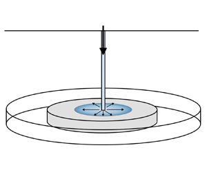
We apply this model to the injection geometry illustrated in figure 3, which considers a radially spreading injection within a confined reservoir of thickness  $H$. As we are considering the initial transient response before the pressure wave reaches the outer boundaries of the reservoir, the reservoir is modelled as infinite. The injection well, of radius
  $r_W$, penetrates the full thickness of the formation. The radial positions of the
  ${\rm CO}_2$ and thermal fronts are
  $r_C(t)$ and
  $r_T(t)$ respectively. The governing equations in terms of the radial distance
  $r$ are then given by
 $$\begin{gather} \beta_f\frac{\partial{p}}{\partial{t}}-\alpha_f\frac{\partial{T}}{\partial{t}}=\frac{kk_r}{\phi_f\mu}\left[\frac{\partial{p}}{\partial{r}}\left(\beta_f\frac{\partial{p}}{\partial{r}} - \alpha_f\frac{\partial{T}}{\partial{r}}\right) + \frac{1}{r}\frac{\partial{ }}{\partial{r}}\left(r\frac{\partial{p}}{\partial{r}}\right)\right], \end{gather}$$
 $$\begin{gather}\overline{\rho c_p}\frac{\partial{T}}{\partial{t}} -\phi_f\alpha_fT\frac{\partial{p}}{\partial{t}} = \rho_fc_{pf}\frac{kk_r}{\mu}\frac{\partial{p}}{\partial{r}}\left(\frac{\partial{T}}{\partial{r}} - \mu_{JT}\frac{\partial{p}}{\partial{r}}\right) + \frac{k_T}{r}\frac{\partial{ }}{\partial{r}}\left(r\frac{\partial{T}}{\partial{r}}\right). \end{gather}$$
Figure 3. Schematic diagram of a radial  ${\rm CO}_2$ injection into a cylindrical
  ${\rm CH}_4$-filled reservoir with thickness
  $H$. The
  ${\rm CO}_2$ and thermal front are denoted
  $r_C$ and
  $r_T$, respectively.
A constant mass flux inner boundary condition can be defined at the wellbore  $r_W$, along with a fixed bottom-hole temperature
  $T_w$. Here we define the problem on an infinite domain, such that the outer boundary maintains the initial reservoir pressure and temperature (
 $p_0, T_0$) as
  $r\rightarrow \infty$. The boundary and initial conditions are then
 $$\begin{gather} \frac{\partial{p}}{\partial{r}}(r_W,t) ={-}\frac{\mu Q}{2{\rm \pi} r_WHkk_r\rho_f}, \quad T(r_W,t) = T_w, \end{gather}$$
 $$\begin{gather}p(\infty,t) = p_0, \quad T(\infty,t) = T_0, \end{gather}$$
where  $Q$ is the mass injection rate through the well (
 ${\rm kg}\ {\rm s}^{-1}$). Note that this represents an idealised injection scenario. During actual injections, the bottom-hole
  ${\rm CO}_2$ conditions depend on
  ${\rm CO}_2$ properties at the well head and on the dynamics of flow within the well. These are likely to vary over time leading to time-dependent boundary conditions.
4.1. Analytical reference solutions
4.1.1. Pressure diffusion
Given low fluid compressibility and small pressure gradients,  $\rho _f$ can be assumed constant and (3.9) can be linearised by neglecting the first and second terms on the right-hand side. Assuming temperature changes are negligible, this leads to the classical pressure diffusion equation (Dake Reference Dake1983; Bear Reference Bear2012)
 \begin{equation} \frac{\partial{p}}{\partial{t}} = \frac{kk_r}{\phi_f\mu\beta_f}\frac{1}{r}\frac{\partial{}}{\partial{r}}\left(r\frac{\partial{p}}{\partial{r}}\right). \end{equation}
Note that in scenarios in which pressure gradients are very high, such as near the wellbore in radially spreading injections, or for fluids with high  $\beta _f$, this linearisation is not appropriate. Comparison of the approximate pressure solution to (4.5) with the fully coupled equations will allow us to explore the effect of the nonlinear terms. Because the temperature and pressure fields vary over a length scale
  $L_p\propto t^{{1}/{2}}$, it is instructive to seek a similarity solution (Barenblatt & Isaakovich Reference Barenblatt and Isaakovich1996) using the similarity variable
 \begin{equation} \eta(r,t) = r\left(4D_pt\right)^{-{1}/{2}} = r\left(\frac{4kk_rt}{\phi\mu\beta_f}\right)^{-{1}/{2}}. \end{equation}
Use of  $\eta$ transforms (4.5) into an ordinary differential equation for the structure of the pressure field:
 \begin{equation} p''+\left(2\eta+\frac{1}{\eta}\right)p' = 0, \end{equation}
where the primes denote derivatives with respect to  $\eta$. Integrating and applying the constant mass flux inner boundary condition gives
 \begin{equation} p' ={-}\frac{\mu Q}{2{\rm \pi} Hkk_r\rho_f\eta}\exp({\eta_W^2-\eta^2}), \end{equation}
where  $\eta _W$ is the value of
  $\eta$ at the wellbore. As the well has a finite and fixed radius,
  $r_W$,
 \begin{equation} \eta_W(t) = r_W\left(\frac{4kk_rt}{\phi\mu\beta_f}\right)^{-{1}/{2}}, \end{equation}
and hence  $\eta _W\rightarrow 0$ as
  $t\rightarrow \infty$. Because we have assumed that
  $\beta _f$ is small and
  $\rho _f$ is relatively constant within the reservoir, we can integrate (4.8) again and apply the far-field outer boundary condition (4.3a,b) to give the similarity solution
 \begin{equation} p = p_0-\frac{\mu Q}{4{\rm \pi} Hkk_r\rho_f}\text{e}^{\eta_W^2}Ei\left(-\eta^2\right), \end{equation}
where  $\rho _f$ is the average fluid density and
  $E_i(y)$ is the exponential integral. We assume a self-similar
  ${\rm CO}_2$ front position, given by
 \begin{equation} r_C(t) = \eta_C\left(\frac{4kk_rt}{\phi\mu\beta_f}\right)^{{1}/{2}}, \end{equation}
where  $\eta _C$ is a numerical constant to be determined. The position of the front can be found by substituting this expression for
  $r_C(t)$ and (4.8) into the expression for the front position (3.18), which gives
 \begin{equation} \eta_C = \left(\frac{\mu\beta_fQ}{4{\rm \pi} Hkk_r\rho_f}\exp({\eta_W^2-\eta_C^2})\right)^{{1}/{2}}. \end{equation}
4.1.2. Steady-state Joule–Thomson cooling
Mathias et al. (Reference Mathias, Gluyas, Oldenburg and Tsang2010) presented an analytical solution for Joule–Thomson cooling, which can be derived if the pressure field is assumed to be in steady state and uncoupled to the temperature field. A truly steady-state pressure field requires mass flux through the outer boundaries to equal that at the injection well. This is a non-physical condition for a cylindrical reservoir with an impermeable caprock, in which the radial symmetry is preserved. However, a pseudo-steady-state condition can be established in a closed reservoir when the pressure wave reaches the outer impermeable boundaries of the reservoir. In this regime  $\partial p/\partial t$ is approximately constant and small over the whole reservoir such that
  $\partial p/\partial r$ at a given radius does not vary substantially with time (Dake Reference Dake1983; Bear Reference Bear2012). The pressure field near the well in the pseudo-steady-state regime can therefore be approximated by
 \begin{equation} \frac{\partial{}}{\partial{r}}\left(r\frac{\partial{p}}{\partial{r}}\right)\simeq 0, \end{equation}
which on imposition of the constant mass flux inner boundary condition gives
 \begin{equation} \frac{\partial{p}}{\partial{r}} ={-}\frac{\mu Q}{2{\rm \pi} Hkk_r\rho_fr}, \end{equation}
where  $\rho _f$ is the average fluid density. Note that, for small
  $r$, this steady-state pressure gradient is the same as the linearised pressure diffusion solution above. If at a given time the wellbore pressure is known to be
  $p_W(t)$ and the reservoir properties can be assumed to be constant, integrating again gives the pressure field as described by Thiem's equation:
 \begin{equation} p = p_W(t)-\frac{\mu Q}{2{\rm \pi} Hkk_r\rho_f}\text{ln}\left(\frac{r}{r_W}\right), \end{equation}
which is recovered from (4.10) as  $r\rightarrow 0$. The radial position of the
  ${\rm CO}_2$ front,
  $r_C$, is found by substituting (4.14) into (3.18) and integrating with respect to time, giving
 \begin{equation} r_C = \left(\frac{Qt}{{\rm \pi} H\phi\rho_f}+r_W^2\right)^{{1}/{2}}\simeq \left(\frac{Qt}{{\rm \pi} H\phi\rho_f}\right)^{{1}/{2}}. \end{equation}
 The temperature field is calculated by coupling this pressure field to a transient temperature equation. Assuming  $\partial p/\partial t$ is small and neglecting heat conduction, substituting (4.14) into (4.2) gives
 \begin{equation} \frac{\partial{T}}{\partial{t}} ={-}\frac{c_{pf}Q}{\overline{\rho c_{p}}2{\rm \pi} Hr}\left(\frac{\partial{T}}{\partial{r}}+\frac{\mu_{JT}\mu Q}{2{\rm \pi} Hkk_r\rho_fr}\right). \end{equation}
Mathias et al. (Reference Mathias, Gluyas, Oldenburg and Tsang2010) solved the temperature equation by applying a Laplace transform. An alternative derivation using intermediate asymptotics is shown in Appendix A, which gives the following solution:
 \begin{equation} T(r,t) = \begin{cases} T_w - \dfrac{\mu_{JT}\mu Q}{2{\rm \pi} H\rho_fkk_r}\text{ln}\left(\dfrac{r}{r_W}\right), & r< r_T,\\ T_0 + \dfrac{\mu_{JT}\mu Q}{4{\rm \pi} H\rho_fkk_r}\text{ln}\left(1-\dfrac{c_{pf}Qt}{\overline{\rho c_p}{\rm \pi} Hr^2}\right), & r>r_T,\\ \end{cases} \end{equation}
where  $r_T$ is the radial position of the thermal front, which is given by
 \begin{equation} r_T = \left[\frac{c_{pf}Qt}{\overline{\rho c_p}{\rm \pi} H} + r_W^2\exp \left(\frac{4{\rm \pi} H kk_r\rho_f(T_w-T_0)}{\mu_{JT}\mu Q}\right)\right]^{{1}/{2}}. \end{equation}
When  $T_w=T_0$, as reported by Mathias et al. (Reference Mathias, Gluyas, Oldenburg and Tsang2010), the front condition is
 \begin{equation} r_T \approx \left[\frac{c_{pf}Qt}{\overline{\rho c_p}{\rm \pi} H} + r_W^2\right]^{{1}/{2}}, \end{equation}
which could equivalently have been derived by substituting the pressure gradient (4.14) into the condition for the thermal front (3.21). Because  $T_w< T_0$ in most injection scenarios, at long times the front condition is better approximated by
 \begin{equation} r_T \approx \left(\frac{c_{pf}Qt}{\overline{\rho c_p}{\rm \pi} H}\right)^{{1}/{2}}=\varGamma^{{1}/{2}}r_C, \end{equation}
where  $\varGamma = {\phi _f\rho _fc_{pf}}/{\overline {\rho c_p}}$ is the fractional volumetric heat capacity. Unlike for the transient pressure field solution above, in which the
  $t^{{1}/{2}}$ dependence arises from the diffusive length scale of the problem, the
  $t^{{1}/{2}}$ dependence of the front positions in the steady-state case arises geometrically due to radial spreading. The maximum degree of Joule–Thomson cooling
  $\Delta T_{JT}$ occurs at the thermal front and is given by
 \begin{equation} \Delta T_{JT} = T_w-T(r_T) = \frac{\mu_{JT}\mu Q}{2{\rm \pi} H\rho_fkk_r}\text{ln}\left(\frac{r_T}{r_W}\right) = \mu_{JT}(p_W-p(r_T)). \end{equation}
In the steady-state case, Joule–Thomson cooling is therefore simply given by  $\mu _{JT}$ multiplied by the pressure drop between the well and thermal front. As the thermal front propagates into the reservoir at a distance
  ${\sim }t^{{1}/{2}}$ through a static logarithmic pressure field, the degree of cooling increases logarithmically with time.
4.2. Transient Joule–Thomson cooling
Given these reference solutions, we now examine the fully coupled model for transient Joule–Thomson cooling. This allows us to quantify the effect of the nonlinear terms and temperature coupling on the pressure field, and the effect of pressure transience on Joule–Thomson cooling.
The consideration of pressure transience requires the solution of the full governing equations, (4.1) and (4.2). A scaling analysis of these equations suggests self-similar solutions in terms of non-dimensional variables for pressure, temperature, radial extent and well radius:
 \begin{align}
&\mathcal{P}= \beta_f
\left(p-p_0\right), \quad \mathcal{T}=
\alpha_f\left(T-T_0\right), \nonumber\\
&\eta = r\left(\frac{4kk_rt}{\phi\mu\beta_f}\right)^{-{1}/{2}},
\quad \eta_W = r_W\left(\frac{4kk_rt}{\phi\mu\beta_f}\right)^{-{1}/{2}},
\end{align}
\begin{align}
&\mathcal{P}= \beta_f
\left(p-p_0\right), \quad \mathcal{T}=
\alpha_f\left(T-T_0\right), \nonumber\\
&\eta = r\left(\frac{4kk_rt}{\phi\mu\beta_f}\right)^{-{1}/{2}},
\quad \eta_W = r_W\left(\frac{4kk_rt}{\phi\mu\beta_f}\right)^{-{1}/{2}},
\end{align}
where  $\eta$ is the similarity variable, and
  $\eta _W$ is a time-dependent variable introduced through the fixed wellbore radius. The initial reservoir pressure and temperature are
  $p_0$ and
  $T_0$, respectively, and
  $\beta _f$ and
  $\alpha _f$ are assumed constant. Substituting the above relations into (4.1) and (4.2) we obtain
 \begin{gather} \frac{\eta_W}{\eta}\left(\frac{\partial{\mathcal{P}}}{\partial{\eta_W}} -\frac{\partial{\mathcal{T}}}{\partial{\eta_W}}\right) + \frac{\partial{\mathcal{P}}}{\partial{\eta}} - \frac{\partial{\mathcal{T}}}{\partial{\eta}} ={-}\frac{1}{2\eta}\left[\frac{\partial{\mathcal{P}}}{\partial{\eta}}\left(\frac{\partial{\mathcal{P}}}{\partial{\eta}} - \frac{\partial{\mathcal{T}}}{\partial{\eta}}\right) +\frac{1}{\eta}\frac{\partial{}}{\partial{\eta}}\left(\eta\frac{\partial{\mathcal{P}}}{\partial{\eta}}\right)\right], \end{gather}
 \begin{gather} \frac{\eta_W}{\eta}\left(\frac{\partial{\mathcal{T}}}{\partial{\eta_W}} -\mathcal{A}\frac{\partial{\mathcal{P}}}{\partial{\eta_W}}\right) + \frac{\partial{\mathcal{T}}}{\partial{\eta}} - \mathcal{A}\frac{\partial{\mathcal{P}}}{\partial{\eta}}\nonumber\\ \quad ={-}\frac{1}{2\eta}\left[\varGamma\frac{\partial{\mathcal{P}}}{\partial{\eta}}\left(\frac{\partial{\mathcal{T}}}{\partial{\eta}}- \mathcal{J}\frac{\partial{\mathcal{P}}}{\partial{\eta}}\right) + \frac{1}{Pe}\frac{1}{\eta}\frac{\partial{}}{\partial{\eta}}\left(\eta\frac{\partial{\mathcal{T}}}{\partial{\eta}}\right)\right]. \end{gather}
Equivalent equations for a fluid with variable  $\beta _f$ and
  $\alpha _f$ are given in Appendix B. The solutions to these equations are self-similar in the far field, but have a slow time dependence in the near-wellbore region due to the requirement to match onto the fixed wellbore radius. The general solutions are therefore
  $\mathcal {P}(\eta,\eta _W)$ and
  $\mathcal {T}(\eta,\eta _W)$. The governing equations are subject to the scaled boundary conditions
 \begin{equation} \mathcal{P}(\infty)=0, \quad \mathcal{T}(\infty)=0, \quad \frac{\partial{\mathcal{P}}}{\partial{\eta}}(\eta_W) ={-}\frac{\chi}{\eta_W}, \quad \mathcal{T}(\eta_W)=\mathcal{T}_W. \end{equation}
The non-dimensional parameters
 \begin{align} \left.\begin{gathered} \varGamma = \frac{\phi\rho_fc_{pf}}{\overline{\rho c_{p}}}, \quad \mathcal{J} = \frac{\alpha_f\mu_{JT}}{\beta_f} = \frac{\left(\left.\dfrac{\partial{T}}{\partial{p}}\right|_H\right)_f}{\left(\left.\dfrac{\partial{T}}{\partial{p}}\right|_{\rho}\right)_f}, \quad \mathcal{A} = \frac{\phi\alpha_f^2 T}{\beta_f\overline{\rho c_p}} = \frac{\left(\left.\dfrac{\partial{T}}{\partial{p}}\right|_S\right)_{f+w+s}}{\left(\left.\dfrac{\partial{T}}{\partial{p}}\right|_{\rho}\right)_f}, \\ Pe = \frac{\overline{\rho c_p}kk_r}{k_T\phi\mu\beta_f} \end{gathered}\right\} \end{align}
depend on fluid and reservoir properties. As defined above,  $\varGamma$ is the volumetric heat capacity ratio of the fluid to the bulk porous medium,
  $\mathcal {J}$ is the scaled Joule–Thomson coefficient of the fluid which controls the magnitude of Joule–Thomson cooling due to flow of the fluid down a pressure gradient,
  $\mathcal {A}$ is the scaled isentropic temperature gradient of the bulk medium which controls the temperature response to transient pressure changes and
  $Pe$ is the thermal Péclet number. The non-dimensional parameters
 \begin{equation} \chi = \frac{\mu\beta_f Q}{2{\rm \pi} Hkk_r\rho_f}, \quad \mathcal{T}_W = \alpha_f\left(T_w-T_0\right), \end{equation}
depend on the boundary conditions at the wellbore.
Note that, as above for the linearised pressure solution, when the domain is rescaled in terms of  $\eta$, the finite well radius causes the position of the inner boundary to be time-dependent,
  $\eta _W=\eta _W(t)$, with
  $\eta _W\rightarrow 0$ as
  $t\rightarrow \infty$. The finite well radius therefore introduces an additional time dependence close to the well. Due to the fixed wellbore temperature, we can make the observation that
 \begin{equation} \frac{\partial{\mathcal{T}}}{\partial{\eta_W}} \simeq{-}\left.\frac{\partial{\mathcal{T}}}{\partial{\eta}}\right|_{\eta\rightarrow\eta_W}, \quad \text{as} \ \eta_W\rightarrow 0. \end{equation}
As observed for the reference solution, the fixed mass injection rate causes the pressure at the wellbore to buildup at a rate inversely proportional to  $\eta _W$, such that the long time solution provides the envelope of the earlier time solutions. In other words, in the absence of temperature coupling, the pressure field is fully self-similar. This means that
 \begin{equation} \frac{\partial{\mathcal{P}}}{\partial{\eta_W}} \simeq 0, \quad \text{as} \ \eta_W\rightarrow 0. \end{equation}
Substituting the above approximations into (4.24) and (4.25) gives
 $$\begin{gather} \mathcal{P}'-\left(1-\frac{\eta_W}{\eta}\right)\mathcal{T}' ={-}\frac{1}{2\eta}\left[\mathcal{P}'\left(\mathcal{P}' - \mathcal{T}'\right) + \frac{1}{\eta}\left(\eta\mathcal{P}'\right) '\right], \end{gather}$$
 $$\begin{gather}\left(1-\frac{\eta_W}{\eta}\right)\mathcal{T}'- \mathcal{A}\mathcal{P}' ={-}\frac{1}{2\eta}\left[\varGamma\mathcal{P}'\left(\mathcal{T}'-\mathcal{J}\mathcal{P}'\right) + \frac{1}{Pe}\frac{1}{\eta}\left(\eta\mathcal{T}'\right)'\right], \end{gather}$$
where the primes now denote derivatives with respect to  $\eta$.
To isolate the effect of temperature coupling on the pressure field, we can additionally consider the solution to the pressure field under isothermal conditions. Employing the same approximations as above, this is described by
 \begin{equation} \mathcal{P}' = \mathcal{P}'^2 + \frac{1}{\eta}\left(\eta\mathcal{P}_i'\right) ', \end{equation}
subject to the boundary conditions
 \begin{equation} \mathcal{P}'(\eta_W(t)) ={-}\frac{\chi}{\eta_W}, \quad \mathcal{P}(\infty) = 0. \end{equation}
4.2.1. Front positions
In the limit  $\eta \gg \eta _W$ the effect of the finite well radius diminishes such that the solution is completely self-similar with respect to the variable
  $\eta$. Hence, the conditions (3.18) and (3.21) for the front positions
  $\boldsymbol {x}_C(t)$ and
  $\boldsymbol {x}_T(t)$ can be rewritten in terms of
  $\eta$ to give
 \begin{equation} \eta_C ={-}\left.\frac{1}{2}\mathcal{P} '\right|_{\eta_C}, \quad \eta_T ={-}\left.\frac{\varGamma}{2}\mathcal{P} '\right|_{\eta_T}, \end{equation}
where  $\eta _C$ and
  $\eta _T$ are the values of
  $\eta$ at the
  $\textrm {CO}_2$ and thermal fronts, respectively. Rearranging the temperature equation, (4.32), we also identify a stationary point in the temperature solution which represents a temperature maximum at
 \begin{equation} \eta_M ={-}\left.\frac{\varGamma\mathcal{J}}{2\mathcal{A}}\mathcal{P} '\right|_{\eta_M}. \end{equation}
Because the conditions (4.34a,b)–(4.36) are only dependent on  $\mathcal {P}$, given a self-similar pressure field, the fronts will be defined for fixed values of
  $\eta _C$,
  $\eta _T$ and
  $\eta _M$. This has the significant benefit that solutions to (4.34a,b) and (4.36) give the positions of the fronts for all time according to
 \begin{equation} r_C = \eta_C\left(\frac{4kk_rt}{\phi\mu\beta_f}\right)^{{1}/{2}}, \quad r_T = \eta_T\left(\frac{4kk_rt}{\phi\mu\beta_f}\right)^{{1}/{2}}, \quad r_M = \eta_M\left(\frac{4kk_rt}{\phi\mu\beta_f}\right)^{{1}/{2}}. \end{equation}
Furthermore, given a self-similar pressure field, the pressures at the fronts,  $\mathcal {P}_C$,
  $\mathcal {P}_T$ and
  $\mathcal {P}_M$, are constant in time.
4.2.2. Numerical approach
We solve (4.31) and (4.32) numerically in python using the scipy.integrate.solve_bvp library, which implements a fourth-order implicit Runge–Kutta method. Due to the time dependence of the inner region, the equations are solved for each time interval of interest, with the inner boundary conditions imposed at  $\eta _W(t)$. The far-field boundary is imposed at a finite
  $\eta$ that is sufficiently large that pressure and temperature gradients are negligible. Varying the position of the outer boundary can be shown to not influence the final solutions.
5. Results
To illustrate the transient Joule–Thomson cooling effect, solutions are calculated for injection into a 2 MPa reservoir with an ambient temperature of  $75\,^{\circ }\textrm {C}$. We consider a constant rate
  $\textrm {CO}_2$ injection at
  $30\ \textrm {kg}\ \textrm {s}^{-1}$ (corresponding to
  $\sim$1 Mt
 $\textrm {CO}_2$ yr
 $^{-1}$) which is relevant to the high injection rates used at
  $\textrm {CO}_2$ sequestration sites such as the Sleipner project (Furre et al. Reference Furre, Eiken, Alnes, Vevatne and Kiær2017). Solutions are calculated for injection temperatures of
  $25\,^{\circ }\textrm {C}$ and
  $75\,^{\circ }\textrm {C}$ to represent a cold and heated injection, respectively.
The reference reservoir and fluid properties are given in table 1. The fluid thermophysical properties  $\rho _r$,
  $\beta _f$,
  $\alpha _f$,
  $c_{pf}$ and
  $\mu$ are assumed to be constant and are calculated using the CoolProp library (Bell et al. Reference Bell, Wronski, Quoilin and Lemort2014) which implements the Span-Wagner equation of state for pure
  $\textrm {CO}_2$. We use a reference pressure
  $p_r$ of 3 MPa and temperature
  $T_r$ equal to that of the wellbore
  $T_w$. Density
  $\rho _f$ is a function of
  $p$ and
  $T$ as given in (3.11). This leads to values of the non-dimensional parameters
  $\varGamma$,
  $\mathcal {A}$,
  $Pe$ and
  $\chi$ which vary as a function of
  $p$ and
  $T$. Reference values for all the non-dimensional parameters at
  $p_r$ and
  $T_r$ are given in table 1.
Table 1. Reference reservoir properties, fluid properties and non-dimensional variables.

The solutions for the cold injection are plotted as a function of  $\eta$ in figure 4 at time intervals up to 1 year, which is the time at which the pressure field would start to interact with the outer boundary of a reservoir with a radius of 2 km. We find that the pressure diffuses smoothly into the reservoir, while the temperature has a sharp advective front which lags behind the injected
  $\textrm {CO}_2$ front due to the thermal inertia of the porous system. Because the fluid density is a function of
  $p$ and
  $T$ we see that it decreases into the reservoir due to decreasing
  $p$, and exhibits a sharp drop across the thermal front due to the increase in
  $T$ at the thermal front. The positions of the
  $\textrm {CO}_2$ front, the thermal maximum and the thermal front occur at constant values of
  $\eta$ for all time. The temperature is self-similar in the far field, but is time-dependent behind the thermal front due to the finite well radius. The maximum amount of cooling increases with time as the pressure drop between the well and thermal front increase. The expanded region shows the small amount of heating ahead of the thermal front due to transient compression of the fluid ahead of the thermal front, with a temperature maximum that lags slightly behind the
  $\textrm {CO}_2$ front. In this case the transient heating is of the order of
  $0.25\,^{\circ }\textrm {C}$.

Figure 4. Example transient solutions, calculated using the reference fluid and reservoir properties (see table 1), for pressure, temperature, density and  $\textrm {CO}_2$ fraction in the mobile fluid phase, plotted against the similarity variable
  $\eta$. Solutions are calculated for a cold injection with
  $T_w=25\,^{\circ }\textrm {C}$. The dotted and dashed lines in the top plot show the uncoupled and linearised pressure field solutions at 1 year. The positions of
  $\eta _W(t)$ at the various times are marked by ‘x’. The positions of
  $\eta _T$,
  $\eta _M$, and
  $\eta _C$ are marked by the vertical blue, orange and grey lines, respectively.
The uncoupled pressure field in addition to the reference analytical solution to the linearised pressure equation are plotted for comparison. the analytical solution assumes a fixed density which we set to the reference density  $\rho _r$. We can evaluate the effect of the nonlinear terms in the pressure equation by comparing the uncoupled
  $p$ field with the analytical reference solution. The analytical
  $p$ field decreases logarithmically with
  $\eta$, while the uncoupled pressure field has more curvature, developing a convex-up shape. This is due to compressibility of the
  $\textrm {CO}_2$ which causes
  $\rho _f$ to increase as
  $p$ builds up around the wellbore. For fixed mass injection rate, higher
  $\rho _f$ of injected
  $\textrm {CO}_2$ causes a reduction in the volumetric injection rate, and therefore a reduction in the pressure gradient at the wellbore over time. The effect of temperature coupling on the pressure field can be evaluated by comparing the uncoupled pressure field with the fully coupled model. The far-field pressure solution is the same as the uncoupled pressure solution, but close to the well it deviates from the uncoupled pressure field due to the sudden jump in
  $\rho _f$ at the thermal front which reduces the near-well pressure gradient in the coupled model. Note that the time dependence of the inner pressure field due to temperature coupling is small.
The solutions for both the cold and hot injection are plotted as a function of  $r$ in figure 5. Also shown for comparison are the analytic steady-state solutions. In a transient flow model the fluid density varies both spatially and temporally due to varying
  $p$ and
  $T$ leading to an ambiguity in the choice of density to use for the steady-state flow solutions when comparing the two models. Steady-state solutions for three different
  $\rho _f$, corresponding to the wellbore densities at the three time intervals, are therefore shown. The choice of density significantly affects the estimate of Joule–Thomson cooling, with the lower and upper bounds of
  $\Delta T_{JT}$ here differing by
  ${\sim }5\,^{\circ }\textrm {C}$. As previously noted by Mathias et al. (Reference Mathias, McElwaine and Gluyas2014), using the steady-state approximation with the wellbore
  $\rho _f$ under-predicts both
  $\Delta T_{JT}$ and the
  $\textrm {CO}_2$ front position
  $r_C$. Despite this, the choice of
  $\rho _f$ for the steady-state solutions has a negligible effect on the estimated position of the thermal front
  $r_T$, and the steady-state models agree with the positions calculated from the transient models. This can be understood from expressions (4.16), (4.20) and (4.22) for the steady-state
  $\textrm {CO}_2$ front, thermal front and maximum Joule–Thomson cooling, respectively. The expressions for the
  $\textrm {CO}_2$ front and the degree of Joule–Thomson cooling explicitly depend on the
  $\rho _f$, whereas the position of the thermal front is dependent on the bulk volumetric heat capacity,
  $\overline {\rho c_{p}}$, which is dominated by the heat capacity of the rock, and thus has a weaker dependence on
  $\rho _f$.

Figure 5. Example transient solutions, calculated using the reference fluid and reservoir properties (see table 1), for pressure, temperature, density and  $\textrm {CO}_2$ fraction in the mobile fluid phase, plotted against the radial distance
  $r$. Solutions are calculated for (a) a cold injection at
  $25\,^{\circ }\textrm {C}$, and (b) a hot injection at
  $75\,^{\circ }\textrm {C}$. The steady-state solutions, calculated using the wellbore densities at the three time intervals, are plotted in dashed lines for comparison.
The transient solutions in figure 5 show a saw-tooth pattern in the near-wellbore temperature field. This is due to the decrease in pressure gradient caused by the decreasing volumetric injection rate over time as  $\rho _f$ at the wellbore increases. This results in gradual heating in the region behind the thermal front due to pressurisation. Here, we have assumed a constant value of
  $\mu _{JT}$. Taking the pressure dependence of
  $\mu _{JT}$ into account, the near-wellbore heating would be more significant than modelled here. This is because
  $\mu _{JT}$ decreases with increasing pressure, which would introduce greater curvature to the inner temperature solution. The transient pressure increase additionally causes minor heating ahead of the thermal front as the pressure wave diffuses into the reservoir. The transient heating is not captured in the steady-state models, as density is assumed to be constant.
5.1. Effects of pressure transience
During the early stages of injection, pressure at any point in the reservoir increases over time due to pressure build up and pressure diffusion into the reservoir. To further explore the effects of this pressure transience it is useful to consider the rate of of change of pressure, temperature and density in both the solid and fluid frames. The rate of change in the fluid frame is given by the material derivative with respect to the fluid velocity  ${\textrm {D}}/{\textrm {D}t} = (\partial d/\partial t+{\boldsymbol {u}}/{\phi }\boldsymbol {\cdot }\boldsymbol {\nabla })$. In figure 6 the rates are plotted as a function of
  $\eta$ so that the profiles at different times can be compared.

Figure 6. Plots of (a) the rate of pressure buildup in the solid frame  $\partial p/\partial t$, (b) the rate of temperature change
  $\partial T/\partial t$, (c) the rate of fluid density increase
  $\partial {\rho _f}/\partial t$, (d) the material derivative of pressure in the fluid frame
  ${\textrm {D}p}/{\textrm {D}t}$, (e) the material derivative of temperature
  ${\textrm {D}T}/{\textrm {D}t}$ and ( f) the material derivative of fluid density
  ${\textrm {D}\rho _f}/{\textrm {D}t}$. All rates are calculated for a cold injection at
  $25 \,^{\circ }\textrm {C}$. The thermal front, temperature maximum and
  $\textrm {CO}_2$ front are marked by blue, red and grey vertical lines, respectively.
In the solid frame, pressure increases over time throughout the reservoir as shown in in figure 6(a). The pressurisation rate is highest at the start of injection and decreases logarithmically with time. The rate of temperature change in the solid frame, is plotted in figure 6(b). As noted above, the region behind the thermal front undergoes compressive heating. Rapid cooling occurs at the thermal front as the solid loses heat to the cold injected fluid. Note that while the degree of cooling increases with time, the rate of cooling is highest at the start of the injection. Ahead of the thermal maximum, the  $\textrm {CO}_2$ and reservoir gas again undergo slight compressive heating. The rate of temperature cycling is important when assessing the risks associated with Joule–Thomson cooling including permeability reduction and formation of gas hydrates. This is because the kinetics of hydrate formation (Farhang, Nguyen & Hampton Reference Farhang, Nguyen and Hampton2014) and the time-dependent creep of reservoir rocks (Brzesowsky et al. Reference Brzesowsky, Hangx, Brantut and Spiers2014) mean that both of these processes are rate-dependent.
Density responds to changes in both pressure and temperature. In figure 6(c) we see that the pressure effect dominates such that at a given point in the reservoir, the fluid density always increases with time. The effect of temperature can be seen at the thermal front, where  ${\textrm {d}\rho }/{\textrm {d}t}$ peaks due to the sudden temperature drop as the cold front advects.
Figure 6(d) shows that  ${\textrm {D}p}/{\textrm {D}t}$ is negative in the fluid frame near the wellbore due to the high fluid velocity around the well, but becomes positive in the far field where both the fluid velocity and pressure gradient are lower. The transition from depressurisation to pressurisation in the fluid frame occurs at the
  $\textrm {CO}_2$ front. Transient pressure increase does work on the fluid causing isentropic heating. The small heated region around the
  $\textrm {CO}_2$ front is thus caused by pressure diffusion into the reservoir where the
  $\textrm {CO}_2$ is nearly immobile. Behind the
  $\textrm {CO}_2$ front, the fluid is flowing faster than the pressure field is diffusing into the reservoir such that the fluid experiences depressurisation as it flows. This explains why the steady-state approximation can be used close to the wellbore: in this region fluid flow is so fast that the pressure field appears static in the fluid frame. In figure 6(e) we see that the fluid undergoes Joule–Thomson cooling in response to the depressurisation around the wellbore. However, the heat content of the solid rock heats the injected fluid and retards the thermal effect. This is observed as heating of the fluid as it crosses the thermal front. The magnitudes of both
  ${\textrm {D}p}/{\textrm {D}t}$ and
  ${\textrm {D}T}/{\textrm {D}t}$ decrease logarithmically with time.
Figure 6( f) shows the material derivative of the fluid density, which from conservation of mass is equivalent to density multiplied by the divergence of the fluid velocity:
 \begin{equation} \frac{\text{D}\rho}{\text{D}t}=\frac{\partial{\rho_f}}{\partial{t}}+\frac{\boldsymbol{u}}{\phi}\boldsymbol{\cdot}\boldsymbol{\nabla}\rho_f ={-}\frac{\rho_f}{\phi}\boldsymbol{\nabla}\boldsymbol{\cdot}\boldsymbol{u}. \end{equation}
Therefore, if  $\boldsymbol {\nabla }\boldsymbol {\cdot }\boldsymbol {u}>0$, the fluid expands as it flows, while if
  $\boldsymbol {\nabla }\boldsymbol {\cdot }\boldsymbol {u}<0$, the fluid contracts. We see that a transition from expansion to contraction occurs at the
  $\textrm {CO}_2$ front and is attributable to the pressurisation ahead of the
  $\textrm {CO}_2$ front. Behind the
  $\textrm {CO}_2$ front the fluid undergoes expansion, with the expansion rate peaking at the thermal front due to heating of the fluid. Behind the thermal front the fluid also undergoes expansion. Given that
 \begin{equation} \frac{\text{D}\rho}{\text{D}t} = \rho_f \left(\beta_f\frac{\text{D}p}{\text{D}t} -\alpha_f\frac{\text{D}T}{\text{D}t}\right), \end{equation}
this is because the effect of pressure decrease outweighs that of temperature decrease due to Joule–Thomson cooling. Applying the steady-state approximation near the wellbore
 \begin{equation} \frac{\text{D}\rho}{\text{D}t} \approx \frac{\rho_f\boldsymbol{u}}{\phi} \left(\beta_f\frac{\partial{p}}{\partial{r}} -\alpha_f\mu_{JT}\frac{\partial{p}}{\partial{r}}\right), \end{equation}
we see that, for pressure to dominate the density field near the wellbore, we must have the condition
 \begin{equation} \frac{\alpha_f\mu_{JT}}{\beta_f}=\mathcal{J}<1. \end{equation}
Whether or not this is the case depends on the fluid properties. As shown in figure 7, for  $\textrm {CO}_2$
  $\mathcal {J}\leq 1$, meaning that
  $\textrm {CO}_2$ will always expand when flowing into a low-pressure reservoir. However, expansion would be minimal for injection near the critical point where
  $(\alpha _f, \beta _f)\rightarrow \infty$.

Figure 7. Phase diagram of  $\textrm {CO}_2$ with contours of
  $\mathcal {J} = {\alpha _f\mu _{JT}}/{\beta _f}$ calculated using the CoolProp library (Bell et al. Reference Bell, Wronski, Quoilin and Lemort2014) for pure
  $\textrm {CO}_2$. At the critical point
  $(\alpha _f, \beta _f)\rightarrow \infty$ such that
  $\mathcal {J}=1$.
5.2. Parametric controls
The behaviour of the non-dimensional pressure and temperature fields is controlled by the non-dimensional parameters  $\varGamma$,
  $\mathcal {J}$,
  $\mathcal {A}$ and
  $Pe$ in addition to the boundary conditions
  $\chi$ and
  $\mathcal {T}_W$. These parameters are functions of the thermodynamic properties of the injected
  $\textrm {CO}_2$ and the reservoir properties and injection conditions. The modes of variability can be observed by varying the parameters independently, as shown in figure 8.

Figure 8. Sensitivity analysis showing parametric controls on pressure and temperature fields of (a) volumetric heat capacity  $\varGamma$, (b) scaled isentropic temperature gradient
  $\mathcal {A}$, (c) scaled Joule–Thomson coefficient
  $\mathcal {J}$, (d) Thermal Péclet number
  $Pe$, (e) scaled wellbore pressure gradient
  $\chi$, ( f) wellbore temperature
  $\mathcal {T}_w$. The black lines show the reference case for injection at
  $75\,^{\circ }\textrm {C}$, and the coloured lines are runs with independently varied parameter values. In plots (a–f) only a single parameter is changed at a time.
Increasing  $\varGamma$ increases the heat capacity of the rock and shifts the position of the thermal front forwards; this slightly increases the degree of cooling. Increasing
  $\mathcal {A}$ increases the amount of compressive heating ahead of the thermal front, but has negligible effect on the degree of Joule–Thomson cooling. Increasing
  $\mathcal {J}$ significantly increases the temperature gradient behind the thermal front and increases the maximum amount of Joule–Thomson cooling
  $\Delta T_{JT}$. Increasing
  $Pe$ sharpens the thermal front and slightly increases
  $\Delta T_{JT}$ at the front. As shown, these parameters have negligible effect on the pressure field.
The parameter  $\chi$ which controls the pressure boundary condition is the only one that has an appreciable effect on the pressure field. Increasing
  $\chi$ increases the wellbore pressure gradient and the rate of pressure buildup. This increases the degree of Joule–Thomson cooling and shifts the thermal front forwards. It also increases the curvature of the pressure field, due to an increased dominance of the nonlinear terms in the pressure equation. Note here that the effect of increasing
  $Q$ has an equivalent effect to increasing the fluid viscosity
  $\mu$ or to decreasing the formation thickness
  $H$ or the permeability
  $k$. Decreasing the temperature boundary condition shifts the temperature field behind the thermal front to lower temperatures. As this increases the density behind the thermal front, It slightly reduces the wellbore pressure gradient.
This parameter variation assumes that each parameter can be varied independently. From an examination of the functional forms of the parameters, which are shown in figure 8, we see that some parameters actually depend on the same reservoir and thermophysical properties. Varying any particular property therefore leads to a combination of the modes of variability shown. For example as porosity  $\phi$ appears in both
  $\varGamma$ and
  $\mathcal {A}$, a larger
  $\phi$ of the reservoir would shift the thermal front forwards, as well as increasing the amount of compressive heating. The permeability
  $k$ is also strongly dependent on
  $\phi$. Increasing
  $k$ would decrease
  $\chi$ and therefore decrease Joule–Thomson cooling and potentially shift the thermal front backwards. Which effect is dominant requires full numerical simulation. The analysis presented here is, however, useful in providing an understanding of the effect the different properties and variables have.
The importance of the different parametric controls in controlling Joule–Thomson cooling depends on the effects shown in figure 8 in addition to the range in values that the parameters are likely to show. Because permeability  $k$ and formation thickness
  $H$ for different reservoirs can vary by up to an order of magnitude, there is scope for
  $\chi$ to vary by up to two orders of magnitude. It is therefore the most important parameter in controlling both the pressure response of the reservoir and the degree of Joule–Thomson cooling. For small, low permeability reservoirs, the injection rate
  $Q$ can be reduced to limit pressure buildup. Variation in parameters
  $\varGamma$,
  $\mathcal {A}$ and
  $\mathcal {J}$ are controlled by the thermophysical properties of the injected
  $\textrm {CO}_2$. The
  $p$ and
  $T$ dependence of these properties introduces additional nonlinearity into the system. While we have not modelled this here, the appropriate scaling for a system with fully variable thermodynamic properties is given in Appendix B. Contours of the equivalent non-dimensional variables
  $\varGamma$,
  $\mathcal {A}$,
  $\mathcal {J}$ and
  $\chi$ (as defined in Appendix B) are plotted on the phase diagram of
  $\textrm {CO}_2$ in figure 9. Parameters
  $\varGamma$ and
  $\mathcal {A}$ attain high values around the critical point. As pressure and temperature vary away from the reservoir, the near-critical
  $p-T$ conditions are likely to only exist over a small radial extent. The parameter
  $\mathcal {J}$ on the other hand varies by up to an order of magnitude between the gas and liquid stability fields due to variation in
  $\mu _{JT}$. We therefore expect much greater Joule–Thomson cooling for a given pressure gradient when injecting in the gas stability field as is the case when injecting into depleted and ultra-depleted reservoirs. Although the fluid density
  $\rho _f$ and viscosity
  $\mu$ trade-off against each other, the parameter
  $\chi$ is also slightly higher, for given injection rate and reservoir properties, in the gas stability field than the liquid field. This further contributes to higher degrees of Joule–Thomson cooling for gas injections.

Figure 9. The  $p-T$ phase diagram of
  $\textrm {CO}_2$ showing the liquid–gas phase transition in the solid black line, and the critical pressure and temperature in the dashed black lines. Contours of (a)
  $\varGamma$, (b)
  $\mathcal {A}$, (c)
  $\mathcal {J}$ and (d)
  $\chi$ calculated using the CoolProp library.
6. Discussion
Joule–Thomson cooling poses significant risks for injection into highly depleted reservoirs. The reduced-order models presented here show cooling of up to  $12\,^{\circ }\textrm {C}$ below that of the wellbore temperature when injecting in the gas stability field. These models are, however, best used as a means of understanding the fundamental physics involved in Joule–Thomson cooling, rather than for developing quantitative operating procedures, for which numerical simulations incorporating the full dependence of thermodynamic properties on reservoir variables can be used. As observed here, the early transient period of injection, in which the pressure wave is propagating into the reservoir, leads to a self-similar pressure field with
  $\textrm {CO}_2$ and thermal fronts which can be described parametrically by self-similar scaling relations. At late times, the maximum degree of Joule–Thomson cooling increases approximately
  $\propto \textrm {ln}(t^{{1}/{2}})$. Therefore, while the cooling rate is most dramatic at the start of injection, the lowest temperatures are predicted to occur at later times. As the greatest degree of cooling occurs immediately behind the thermal front, the cold region expands out as an annulus away from the wellbore as illustrated in figure 5. The risks associated with very low temperatures, including freezing of pore waters, and formation of gas hydrates are therefore expected to occur immediately behind the thermal front. Because the pressure gradient is greatest in the region closest to the wellbore, the risks associated with the clogging of pore-space and the accompanying permeability reduction, such as failure of the caprock, are somewhat mitigated by the lowest temperatures occurring at greater radial distances where pressure gradients are lower.
Transient cooling continues until the point when the pressure wave interacts with the boundaries of the reservoir. Due to heterogeneities within geological reservoirs this pressure boundary could correspond to a sealed fault or a region of lower permeability arising from lithological variation. The effect of a closed outer boundary was not simulated here, but it may be anticipated that once the pressure field impinges on the outer boundary, the pressure will build up across the whole reservoir resulting in compressive heating.
The  $p-T$ trajectories of the reference models with injection temperatures of
  $25\,^{\circ }\textrm {C}$ and
  $75\,^{\circ }\textrm {C}$ are plotted in figure 10. The open circles mark the wellbore
  $p-T$ conditions. Note that the wellbore temperature
  $T_w$ remains constant due to the fixed temperature boundary condition imposed, while the pressure increases over time due to pressure build-up at the well. The closed circle marks the far-field reservoir conditions, which remain fixed over time. The radial Joule–Thomson cooling paths have a characteristic ‘hooked’ shape. From the wellbore they initially trace a linear path with positive
  $p-T$ slope. This represents the region behind the thermal front. Neglecting the effect of transient compressive heating, the temperature gradient is approximated by
  $\partial T/\partial p\approx \mu _{JT}$. The linear slope of this segment therefore arises from the use of a constant value of
  $\mu _{JT}$. The
  $p-T$ dependence of
  $\mu _{JT}$ would actually create curvature of these paths. Following this initial linear slope, there is a quasi-isobaric increase in temperature, which corresponds to heating of the
  $\textrm {CO}_2$ across the thermal front. An important result from this work is that at late times, the pressure at the thermal front is approximately constant over time. This is due to the self-similarity of both the pressure field and the thermal front position, as observed in figure 4. Following the rapid temperature increase there is a smooth transition to an approximately isothermal pressure drop until the far-field reservoir pressure is reached. The
  $p-T$ path actually slightly over-shoots the reservoir temperature due the compressive heating around the
  $\textrm {CO}_2$ front, however, this is hard to discern in the plots shown here.

Figure 10. The  $p-T$ phase diagram of
  $\textrm {CO}_2$, with the liquid–gas phase transition in solid black line, and the critical pressure and temperature marked in dashed black lines. The phase boundaries for
  $\textrm {CO}_2$ and
  $\textrm {CH}_4$-hydrate and pure H
 $_2$O ice are marked, with the freezing window shaded in blue. The
  $p-T$ trajectories for the low-
 $T$ (
$T$ ( $T_W=25^{\circ }$C) and high-
 $T$ (
$T$ ( $T_W=75\,^{\circ }\textrm {C}$) injections are shown at 3 different times. The dashed lines show a low-
 $T$ injection with a higher injection rate. The wellbore pressure and temperature are marked by the open circles and the far-field reservoir conditions are marked by the closed circle.
We have also plotted the stability fields for  $\textrm {CO}_2$ and
  $\textrm {CH}_4$-hydrates using data from Sun & Duan (Reference Sun and Duan2005), in addition to the water–ice phase transition for pure water using data from the Engineering Toolbox (www.engineeringtoolbox.com). Gas hydrates are a type of crystalline ice composed of
  $\textrm {CO}_2$ or
  $\textrm {CH}_4$ molecules enclosed within a solid H
 $_2$O lattice. As an example we have plotted the
  $p-T$ trajectory of a low-
 $T$ injection in which the injection rate
  $Q$ is doubled to
  $60\ \textrm {kg}\ \textrm {s}^{-1}$. All other parameters are as given in table 1. In this example, the greater pressure buildup causes the
  $p-T$ conditions to enter into the hydrate stability field after 1 year of injection, resulting in a partially frozen annulus. Freezing of pore water and formation of gas hydrates causes a reduction in permeability. This has the effect of restricting fluid flow and reducing the pressure diffusivity, which would cause a buildup of pressure behind the low-permeability annular hydrate zone. The extent of permeability reduction caused by hydrate formation would depend on both the pore volume occupied by hydrates (Almenningen et al. Reference Almenningen, Gauteplass, Hauge, Barth, Fernø and Ersland2019), and their pore-scale distribution (Kleinberg et al. Reference Kleinberg, Flaum, Griffin, Brewer, Malby, Peltzer, Yesinowski and Griffin2003). In the limit of severe permeability reduction, the cooled annular region would act as a sealed barrier, with the effect of restricting the radial extent of the reservoir. Since
  $\textrm {CO}_2$ hydrates are >70 wt%
  $\textrm {H}_2\textrm {O}$ (Sun & Kang Reference Sun and Kang2016), in practice, the volume fraction of hydrate that can form depends on the availability of water. In dry gas reservoirs, in which gas saturation is high, permeability reduction is unlikely to be significant. Furthermore,
  $\textrm {CO}_2$ injection is a drying process which creates a dry-out front around the wellbore. However, because the dry-out front propagates into the reservoir more slowly than the thermal front (Creusen Reference Creusen2018), it can be assumed that there will be some water available for hydrate formation within the low-temperature region. To date there is no literature modelling the dynamic and geomechanical consequences of hydrate formation in depleted reservoirs. Further work targeted at specific case studies is required to understand the potential effects of hydrate formation. Since the effect of hydrate formation on injectivity and reservoir stability is yet to be assessed, a conservative injection strategy is to ensure that pressure and temperature in the near-wellbore region remain outside of the hydrate formation window.
As demonstrated in the sensitivity analysis, the key parameters controlling the degree of cooling are permeability, reservoir size, injection rate and the Joule–Thomson coefficient. As the minimum temperature is given by  $T_{min}=T_W-\Delta T_{JT}$, the wellbore temperature
  $T_W$ is also important. For moderate to low fluid compressibility, the minimum temperature reached can be approximated by the analytical solution for steady-state flow, which gives
 \begin{equation} T_{min} = T_W - \frac{\mu_{JT}\mu Q}{4{\rm \pi} H\rho_fkk_r}\text{ln}\left(\frac{c_{pf}Qt}{\overline{\rho c_p}{\rm \pi} Hr_w^2}+1\right). \end{equation}
This highlights the parametric controls. Thus, high injection rates, low permeabilities and very low injection temperatures should be avoided. Care should also be taken when injecting  $\textrm {CO}_2$ in the gas stability field.
Figure 10 also shows the  $\textrm {CO}_2$ liquid–gas phase transition. The models presented here for the early transient phase of injection remain within the gas stability field. As noted in § 5.2, the high Joule–Thomson coefficient and low density of
  $\textrm {CO}_2$ gas are expected to cause more significant pressure buildup and Joule–Thomson cooling than when injecting liquid
  $\textrm {CO}_2$. In all of the models presented here pressure buildup is insufficient to cause
  $p-T$ conditions to enter the liquid stability field within the first year of injection. However, sustained high mass injection rates are likely to result in a liquid–gas phase transition either within the well, or within the reservoir. In an adiabatic system, we expect the
  $p-T$ path to be buffered along the phase boundary such that there is a finite region in which liquid and gas coexist. Self-consistent inclusion of the phase transition therefore requires equations for multiphase flow, as well as the thermodynamic effects of the latent heat of vaporisation and volume change of reaction. The relative thermal effects of latent heat of vaporisation and Joule–Thomson cooling are yet to be explored.
In this analysis we have considered injection into a homogeneous reservoir. Sedimentary rocks are highly heterogeneous on both large and small scales, and are often comprised of layers of varying permeability reflecting lithological variation, bedding planes, cross-bedding and variable mineralisation. The influence of spatially correlated heterogeneity on  $\textrm {CO}_2$ plume migration and trapping efficiency has been extensively studied (e.g. Lengler, De Lucia & Kühn Reference Lengler, De Lucia and Kühn2010; Benham, Bickle & Neufeld Reference Benham, Bickle and Neufeld2021) and fluid flow has been shown to be focused within high-permeability layers. One way to apply the models presented here to understand Joule–Thomson cooling within a layered heterogeneous medium is to consider a horizontally layered rock in which the vertical permeability
  $k_v=0$, such that flow is only in the horizontal plane. The pressure diffusivity
  $D_p = {kk_r}/{\phi \mu \beta _f}$ is lower in low-permeability layers, such that the speed of the pressure propagation scales
  ${\sim }k^{{1}/{2}}$. From the analytical pressure diffusion solution and the sensitivity analysis, we also know that the pressure gradient scales
  ${\sim }k^{-1}$. For the same injection rate across all layers, pressure build-up and near-wellbore pressure gradients will be larger in the low permeability layers. This will result in enhanced Joule–Thomson cooling and a greater probability of hydrate formation in low-permeability layers. An interesting repercussion is therefore that Joule–Thomson cooling could reduce permeability in low-permeability layers and further enhance heterogeneity. This would increase flow localisation in high-permeability layers. Note, however, that this neglects vertical fluid flow, sometimes referred to as pressure leakage. In practice vertical thicknesses are small compared with lateral reservoir extent, meaning that pressure could equilibrate quickly across layers. The pressure diffusivity is therefore more likely to be set by the average permeability across all layers.
7. Conclusions
The results here explore the thermal effects of compressible flow during  $\textrm {CO}_2$ injection into depleted gas-filled reservoirs. During the early transient injection phase, when the pressure wave is propagating into the reservoir, before having interacted with the outer boundary, the pressure and temperature fields can be described by similarity solutions. Pressure and temperature propagate radially into the reservoir
  $\propto t^{{1}/{2}}$. The rate of propagation is set by the diffusivity of the pressure field which depends on the fluid compressibility. The
  $\textrm {CO}_2$ front and thermal front, which lags behind the
  $\textrm {CO}_2$ front, also scale with the pressure diffusion length scale.
Unlike steady-state flow, transient injection causes both heating and cooling. Joule–Thomson cooling occurs due to flow down the pressure gradient, which leads to rapid cooling of the reservoir across the thermal front. Transient pressure increase causes slight warming of the reservoir around the  $\textrm {CO}_2$ front, and behind the thermal front, after the thermal front has passed. The models presented provide a tool for understanding the fundamental physics of Joule–Thomson cooling, and for determining the important parametric controls. Safe injection requires that temperature and pressure remain outside the hydrate stability field. In accordance with previous studies, we find that the crucial parameters controlling the minimum temperatures reached are injection rate, wellbore temperature, reservoir permeability and thickness, Joule–Thomson coefficient and fluid density.
Improved understanding of the  $p-T$ behaviour during injection into depleted reservoirs requires inclusion of the liquid–gas phase transition, as well as the full
  $p-T$ dependence of the thermodynamic properties. Future work should focus on these effects.
Funding
This work was supported by the Department for Net Zero and Energy Security as part of the RETURN project (grant number G117196) through the Accelerating CCS Technologies (ACT) programme.
Declaration of interests
The authors report no conflict of interest.
Data availability
The data that support the findings of this study are available within the article.
Appendix A
For a steady-state radial injection, the temperature field is described by (4.17). Close to the well, radial distance and temperature can be scaled as follows:
 \begin{equation} \lambda = \frac{r}{r_W}, \quad \mathcal{T} = \frac{2{\rm \pi} Hkk_r\rho_f(T-T_0)}{\mu_{JT}\mu Q}, \quad \mathcal{T}_W = \frac{2{\rm \pi} Hkk_r\rho_f(T_W-T_0)}{\mu_{JT}\mu Q}. \end{equation}
Substituting these variables into (4.17) leads to
 \begin{equation} \frac{\overline{\rho c_p}2{\rm \pi} Hr_W^2}{c_{pf} Q}\frac{\partial{\mathcal{T}}}{\partial{t}} = \frac{1}{\lambda}\left(\frac{\partial{\mathcal{T}}}{\partial{\lambda}}+\frac{1}{\lambda}\right). \end{equation}
In the limit  $r_W\rightarrow 0$, the temperature field close to the well is approximated by
 \begin{equation} \frac{\partial{\mathcal{T}}}{\partial{\lambda}} ={-}\frac{1}{\lambda}. \end{equation}
Integrating and applying the constant wellbore temperature boundary condition gives
 \begin{equation} \mathcal{T} = \mathcal{T}_W-\text{ln}(\lambda), \end{equation}
which can be expressed dimensionally as
 \begin{equation} T = T_W - \frac{\mu_{JT}\mu Q}{2{\rm \pi} Hkk_r\rho_f}\text{ln}\left(\frac{r}{r_W}\right). \end{equation}
 Far from the well, we expect the solution to be self-similar with respect to the similarity variable  $\zeta$, defined as
 \begin{equation} \zeta = \frac{\overline{\rho c_p}2{\rm \pi} Hr^2}{c_{pf}Qt}. \end{equation}
Substituting this into (4.17) leads to
 \begin{equation} \frac{\partial{\mathcal{T}}}{\partial{\zeta}} = \frac{1}{\zeta(\zeta-2)}. \end{equation}
Integrating and applying the far-field boundary condition gives
 \begin{equation} \mathcal{T} = \frac{1}{2}\text{ln}\left(\frac{\zeta-2}{\zeta}\right), \end{equation}
which can be expressed dimensionally as
 \begin{equation} T = T_0 + \frac{\mu_{JT}\mu Q}{4{\rm \pi} Hkk_r\rho_f}\text{ln}\left(1-\frac{c_{pf}Qt}{\overline{\rho c_p}{\rm \pi} Hr^2}\right). \end{equation}
 Solutions (A5) and (A9) can be matched across the thermal front, such that the position of the thermal front,  $r_T$, is given by equating (A5) and (A9), which leads to
 \begin{equation} r_T = \left[\frac{c_{pf}Qt}{\overline{\rho c_p}{\rm \pi} H} + r_W^2\exp\left(\frac{4{\rm \pi} H kk_r\rho_f(T_w-T_0)}{\mu_{JT}\mu Q}\right)\right]^{{1}/{2}}. \end{equation}
Appendix B
For fluids with variable compressibility  $\beta _f$ and expansivity
  $\alpha _f$ we may use the following scalings:
 \begin{align}
&\mathcal{P}= \beta_r
\left(p-p_0\right), \quad \mathcal{T}=
\alpha_r\left(T-T_0\right),\nonumber\\
& \eta = r\left(\frac{4kk_rt}{\phi\mu\beta_r}\right)^{-{1}/{2}},\quad
\eta_W = r_W\left(\frac{4kk_rt}{\phi\mu\beta_r}\right)^{-{1}/{2}},
\end{align}
\begin{align}
&\mathcal{P}= \beta_r
\left(p-p_0\right), \quad \mathcal{T}=
\alpha_r\left(T-T_0\right),\nonumber\\
& \eta = r\left(\frac{4kk_rt}{\phi\mu\beta_r}\right)^{-{1}/{2}},\quad
\eta_W = r_W\left(\frac{4kk_rt}{\phi\mu\beta_r}\right)^{-{1}/{2}},
\end{align}
where  $\beta _r$ and
  $\alpha _r$ are the reference compressibility and expansivity, respectively. Substituting the above relations into (4.1) and (4.2) and assuming the solutions are in steady state with respect to
  $\eta$ we obtain
 $$\begin{gather} \tilde{\beta}_f\mathcal{P}'-\left(1-\frac{\eta_W}{\eta}\right)\tilde{\alpha}_f\mathcal{T}' ={-}\frac{1}{2\eta}\left[\mathcal{P}'\left(\tilde{\beta}_f\mathcal{P}' - \tilde{\alpha}_f\mathcal{T}'\right) + \frac{1}{\eta}\left(\eta\mathcal{P}'\right) '\right], \end{gather}$$
 $$\begin{gather}\left(1-\frac{\eta_W}{\eta}\right)\mathcal{T}'- \mathcal{A}\mathcal{P}' ={-}\frac{1}{2\eta}\left[\varGamma\mathcal{P}'\left(\mathcal{T}'-\mathcal{J}\mathcal{P}'\right) + \frac{1}{Pe}\frac{1}{\eta}\left(\eta\mathcal{T}'\right)'\right], \end{gather}$$
subject to the boundary conditions, as given in (4.26a–d). The non-dimensional parameters for fluids with variable  $\beta _f$ and
  $\alpha _f$ are then
 \begin{equation} \left.\begin{gathered} \varGamma = \frac{\phi\rho_fc_{pf}}{\overline{\rho c_{p}}}, \quad \mathcal{J} = \frac{\alpha_r\mu_{JT}}{\beta_r}, \quad \mathcal{A} = \frac{\phi\alpha_r\alpha_f T}{\beta_r\overline{\rho c_p}}, \quad Pe = \frac{kk_r\overline{\rho c_p}}{k_T\phi\mu\beta_f},\\ \tilde{\beta}_f = \frac{\beta_f}{\beta_r}, \quad \tilde{\alpha}_f = \frac{\alpha_f}{\alpha_r}, \quad \chi = \frac{\mu\beta_r Q}{2{\rm \pi} Hkk_r\rho_f}, \quad \mathcal{T}_W = \alpha_r\left(T_w-T_0\right), \end{gathered}\right\} \end{equation}
where the additional parameters  $\tilde {\beta }_f$ and
  $\tilde {\alpha }_f$ describe the
  $p-T$ variation of
  $\beta _f$ and
  $\alpha _f$.


 Open access