


1. Introduction
With the rapid increase of robots landing in various fields, robots inevitably interact with the external environment in contact-rich applications such as assembly automation and human–robot collaboration [Reference Jiang, Yao, Huang, Yu, Wang and Bi1, Reference Mukherjee, Gupta, Chang and Najjaran2]. However, the environment is usually unknown and uncertain in these scenarios, making it quite challenging to ensure safe and effective interactions during the tasks. In the existing research, two methods have been widely used to achieve compliant interaction behaviors between manipulators and the environment. The first method is hybrid position/force control proposed by Raibert and Craig [Reference Raibert and Craig3], which decomposes the task space into position-controlled and force-controlled subspaces but will easily result in the instability of the interaction when the modeling accuracy of the environment or robot dynamics is insufficient. The second method is impedance control proposed by Hogan [Reference Hogan4], whose goal is to establish a dynamical relationship between the motion of the manipulator and the interaction force, rather than controlling these variables separately. Moreover, impedance control has proven to be easier to implement and more robust [Reference Song, Yu and Zhang5].
In impedance control, obtaining the target impedance model which describes the desired interaction behavior is necessary. A basic approach is to impose a passive impedance model on the manipulator, which can guarantee the interaction stability under any passive environment [Reference Colgate and Hogan6]. Further, the environment dynamics were considered since the model’s passivity cannot guarantee that the manipulator can adapt to the environment [Reference Buerger and Hogan7]. The adaptive impedance controllers using polynomial universal approximators and q-Chlodowsky operators to approximate the system uncertainties, unmodeled dynamics, and external disturbances were designed in refs. [Reference Izadbakhsh and Khorashadizadeh8, Reference Izadbakhsh, Deylami and Khorashadizadeh9]. However, obtaining an impedance model that matches the environment is difficult since the environment dynamics are usually unknown. Moreover, a fixed target impedance model is not applicable in many flexible tasks such as human–robot collaboration [Reference Sharkawy and Koustoumpardis10, Reference Jin, Qin, Liu, Zhang and Yu11], so a variable admittance control approach was proposed by ref. [Reference Sharkawy, Koustoumpardis and Aspragathos12] to tune the inertia and provide the robot with the adaptive ability to cope with different task states in human–robot cooperation. In ref. [Reference Roveda, Riva, Bucca and Piga13], a sensorless optimal switching impact/force controller with impedance adaptive mechanism was proposed to realize stable free-space/contact phase control of the robot. In ref. [Reference Roveda, Shahid, Iannacci and Piga14], a sensorless model-based method was proposed to estimate the environmental stiffness and tune impedance gains online. A Q-Learning-based model predictive variable impedance controller was developed, which can learn the human–robot interaction dynamics and uncertainties and optimize the impedance parameters [Reference Roveda, Testa, Shahid, Braghin and Piga15]. Therefore, iterative learning was utilized to update the impedance parameters iteratively through repeated contact operations of the manipulator, leading to the desired impedance model adapted to the unknown environment [Reference Li and Ge16]. The reference adaptation approach was used to parameterize the desired trajectory and iteratively search for the optimal parameter to obtain the desired interaction performance [Reference Peng, Chen and Yang17]. However, the repeated operations in iterative learning are inflexible and time-consuming, so the impedance adaptation which has the potential to obviate the repeated operations of the manipulator has been focused on. In ref. [Reference Zeng, Yang and Chen18], a bioinspired approach derived from human motor learning was proposed to adapt the impedance and feedforward torque in the unknown and dynamic environment to meet the requirements of interaction. In ref. [Reference Qiao, Zhong, Chen and Wang19], the advanced research on human-inspired intelligent robots was summarized and a significant insight into the principle of human-like impedance adaptation for robots was provided. Further, a brain-inspired intelligent robotic system was established in ref. [Reference Qiao, Wu, Zhong, Yin and Chen20], which strongly proved the effectiveness of human-like impedance adaptation for improving the performance of robots.
In general, the target impedance model discussed above corresponds to a good trade-off between trajectory tracking and interaction force regulation obtained by optimization. When the environment dynamics are known, the optimal impedance parameters can be easily obtained using the well-known linear quadratic regulator (LQR). However, LQR is not suitable for unknown linear systems caused by unknown environment dynamics [Reference Lewis, Vrabie and Syrmos21]. Hence, adaptive dynamic programming (ADP), as a method to design the optimal controller with only partial information of the controlled system model, has attracted wide attention [Reference Wang, Zhang and Liu22]. Based on the ADP approach in ref. [Reference Jiang and Jiang23], an impedance adaptation method was proposed to obtain the target impedance parameters that guarantee the optimal interaction in the unknown environment without repeated operations of the manipulator [Reference Ge, Li and Wang24]. As an improvement of ref. [Reference Ge, Li and Wang24], an auxiliary function was designed in the impedance adaptation to make the feedback gain change smoothly, and the broad fuzzy neural network and the barrier Lyapunov function were used to deal with the uncertainty of robot dynamics and the state constraint problem [Reference Huang, Yang and Chen25]. In ref. [Reference Yang, Peng, Li, Cui, Cheng and Li26], an admittance adaptation method was proposed for the unknown environment, where a torque observer was employed and an advanced adaptive controller was designed to ensure trajectory tracking performance. However, in the second-order environment, namely the mass–spring–damper environment, the methods in refs. [Reference Ge, Li and Wang24–Reference Yang, Peng, Li, Cui, Cheng and Li26] can only obtain a first-order target impedance model, namely spring–damper model, which has a limited range to describe the interaction behavior and thus is not suitable for many tasks.
In practice, not only the acquisition of the target impedance model but also its implementation should be considered carefully, both of which ensure the desired interaction behavior of the manipulator interacting with the environment. According to the different causality, impedance control can be implemented in two ways, which are referred to as “impedance control” and “admittance control.” In essence, these two controllers have complementary stability and performance due to their fixed causality [Reference Valency and Zacksenhouse27, Reference Ott, Mukherjee and Nakamura28], which is qualitatively shown in Fig. 1. To be specific, due to the inability of impedance control to provide stiff behavior, impedance control results in poor position accuracy in free motion and soft environments affected by uncompensated frictions, but it can guarantee stability and provide good performance in interaction with stiff environments. On the contrary, admittance control results in poor robustness and even instability in stiff environments due to its stiff characteristic but can compensate for unmodeled frictions and provide high position accuracy in free motion and soft environments.
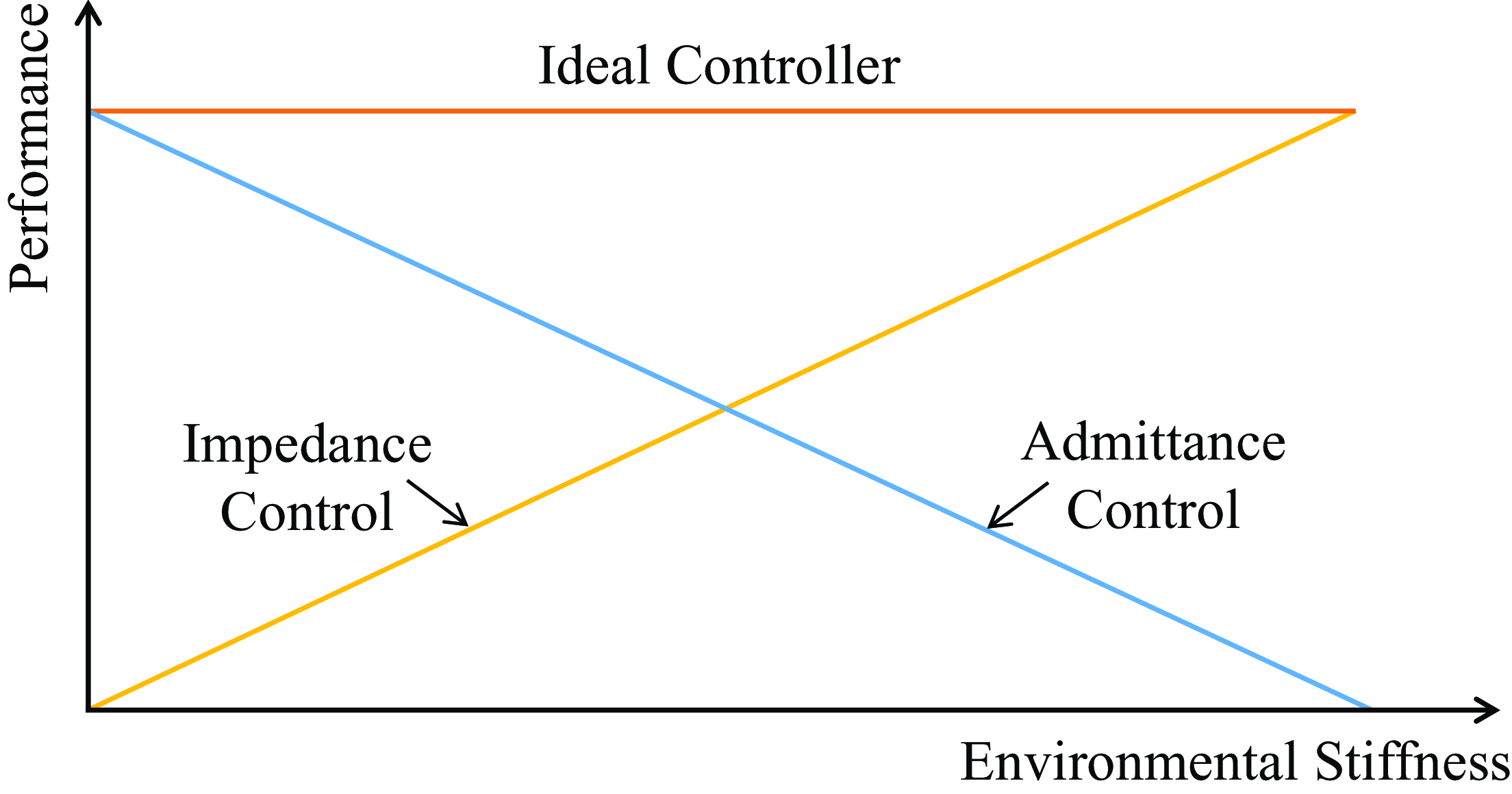
Figure 1. Qualitative representation of impedance and admittance controllers performance. Neither of these two controllers is well adapted to a wide range of environmental stiffness, so it is necessary to design an ideal controller that can provide good performance in any environment stiffness [Reference Ott, Mukherjee and Nakamura28].
To cope with this problem, Ott, Mukherjee, and Nakamura proposed a hybrid system framework to achieve the performance of the ideal controller in Fig. 1 [Reference Ott, Mukherjee and Nakamura28, Reference Ott, Mukherjee and Nakamura29]. By utilizing the switching controller according to the switching period and duty cycle, the framework interpolates between the responses of impedance control and admittance control and provides good performance in a wide range of environmental stiffness. As an improvement of ref. [Reference Ott, Mukherjee and Nakamura29], a hybrid controller that can adapt the switching period and duty cycle was developed to improve the control performance [Reference Formenti, Bucca, Shahid, Piga and Roveda30]. In ref. [Reference Rhee, Kang, Moon, Choi and Choi31], a hybrid control strategy was proposed, where the switch between impedance and admittance controllers was triggered by the position error, which led to good performance under any impedance condition. To obtain the optimal implementation performance of the target impedance model in different environments, an adaptive hybrid system framework was proposed by ref. [Reference Cavenago, Voli and Massari32] using the neural network based on ref. [Reference Ott, Mukherjee and Nakamura29], which directly established the mapping of the states and force of the robot to the optimal duty cycle to obtain the intermediate controller that provided the optimal performance in a fixed or time-varying environment. It is worth noting that although environmental stiffness is the main factor affecting the performance of impedance and admittance controllers, environmental inertia and damping in the second-order environment also need to be considered since they greatly affect the system stability. However, the above approaches consider neither the acquisition of the optimal impedance model nor the interaction with the second-order environment.
According to the above discussion, this article proposes a hybrid impedance and admittance control (HIAC) scheme to address two problems. The first problem is that existing impedance adaptation methods [Reference Ge, Li and Wang24–Reference Yang, Peng, Li, Cui, Cheng and Li26] can only obtain insufficient first-order impedance models in the second-order unknown environment. The second problem is that existing hybrid control methods [Reference Ott, Mukherjee and Nakamura28–Reference Cavenago, Voli and Massari32] do not consider the interaction with the second-order environment. Therefore, this inspires us to propose a unified scheme to optimally obtain and implement the target impedance model for the manipulator subjected to the second-order unknown environment. It should be noted that although the uncertainties and environment dynamics lead to differences in the performance of impedance control and admittance control due to their different causality, our goal is not to compensate for system uncertainties like conventional adaptive impedance control but to utilize the hybrid system framework to provide optimal consistent impedance implementation performance independent of the environmental stiffness under unknown uncertainties and the second-order environment. Compared with the existing research, the main contributions of this article are summarized below:
-
1. An impedance adaptation method with virtual inertia is proposed to obtain the second-order target impedance model representing the optimal interaction behavior in the second-order unknown environment without the accurate environment dynamics and acceleration feedback.
-
2. A hybrid system framework suitable for the second-order environment is proposed to implement the target impedance model with its stability analyzed.
-
3. A mapping of the optimal duty cycle is built to select the optimal intermediate controller to provide the optimal implementation performance for the obtained target impedance model.
The rest of this article is organized as follows. In Section 2, the preliminaries including the robot and environment dynamics, LQR, and impedance control and admittance control are introduced. Section 3 introduces the methodologies containing the adaptive optimal control, impedance adaptation, and hybrid system framework with its stability analysis and mapping of the optimal duty cycle. Simulation and experimental studies are conducted in Section 4 and 5 to verify the effectiveness of the proposed HIAC scheme, respectively. Section 6 gives the conclusions.
2. Preliminaries
2.1. System model
For the system, we consider that an n-DOF rigid robot manipulator is in interaction with an environment. The forward kinematics of the manipulator is given first:
 \begin{equation} \boldsymbol{x}=\phi (\boldsymbol{q}) \end{equation}
where
 $\boldsymbol{x}$
and
$\boldsymbol{x}$
and
 $\boldsymbol{q}\in \mathbb{R}^n$
denote the end-effector’s coordinates in Cartesian space and joint angle vector in joint space, respectively. Differentiating (1) along time yields
$\boldsymbol{q}\in \mathbb{R}^n$
denote the end-effector’s coordinates in Cartesian space and joint angle vector in joint space, respectively. Differentiating (1) along time yields
 \begin{equation} \dot{\boldsymbol{x}}={\boldsymbol{J}}(\boldsymbol{q})\dot{\boldsymbol{q}} \end{equation}
where
 ${\boldsymbol{J}}(\boldsymbol{q})$
is the Jacobian matrix. Differentiating (2) along time, we have
${\boldsymbol{J}}(\boldsymbol{q})$
is the Jacobian matrix. Differentiating (2) along time, we have
 \begin{equation} \ddot{\boldsymbol{x}}=\dot{{\boldsymbol{J}}}(\boldsymbol{q})\dot{\boldsymbol{q}}+{\boldsymbol{J}}(\boldsymbol{q})\ddot{\boldsymbol{q}}. \end{equation}
The nominal dynamics of the robot manipulator without considering the uncertainties and frictions in joint space are given by ref. [Reference Zeng, Yang and Chen18]:
 \begin{equation} {\boldsymbol{H}}(\boldsymbol{q})\ddot{\boldsymbol{q}}+{\boldsymbol{C}}(\boldsymbol{q},\dot{\boldsymbol{q}})\dot{\boldsymbol{q}}+{\boldsymbol{G}}(\boldsymbol{q})=\boldsymbol{\tau}_{\boldsymbol{c}}+{\boldsymbol{J}}^T(\boldsymbol{q})\boldsymbol{F}_{\boldsymbol{e}} \end{equation}
where
 ${\boldsymbol{H}}(\boldsymbol{q})\in \mathbb{R}^{n\times{n}}$
is the inertia matrix.
${\boldsymbol{H}}(\boldsymbol{q})\in \mathbb{R}^{n\times{n}}$
is the inertia matrix.
 ${\boldsymbol{C}}(\boldsymbol{q},\dot{\boldsymbol{q}})\dot{\boldsymbol{q}}\in \mathbb{R}^n$
is the Coriolis and Centrifugal force vector.
${\boldsymbol{C}}(\boldsymbol{q},\dot{\boldsymbol{q}})\dot{\boldsymbol{q}}\in \mathbb{R}^n$
is the Coriolis and Centrifugal force vector.
 ${\boldsymbol{G}}(\boldsymbol{q})\in \mathbb{R}^n$
is the gravitational force vector.
${\boldsymbol{G}}(\boldsymbol{q})\in \mathbb{R}^n$
is the gravitational force vector.
 $\boldsymbol{\tau}_{\boldsymbol{c}}\in \mathbb{R}^n$
is the control torque input vector, and
$\boldsymbol{\tau}_{\boldsymbol{c}}\in \mathbb{R}^n$
is the control torque input vector, and
 $\boldsymbol{F}_{\boldsymbol{e}}\in \mathbb{R}^n$
denotes the force applied by the external environment. Since the interaction is conducted in Cartesian space, the robot dynamics in joint space is transformed to Cartesian space to simplify the analysis. Integrating (2) and (3) into (4), the nominal robot dynamics in Cartesian space can be described by:
$\boldsymbol{F}_{\boldsymbol{e}}\in \mathbb{R}^n$
denotes the force applied by the external environment. Since the interaction is conducted in Cartesian space, the robot dynamics in joint space is transformed to Cartesian space to simplify the analysis. Integrating (2) and (3) into (4), the nominal robot dynamics in Cartesian space can be described by:
 \begin{equation} {\boldsymbol{H}}_{\boldsymbol{x}}(\boldsymbol{q})\ddot{\boldsymbol{x}}+{\boldsymbol{C}}_{\boldsymbol{x}}(\boldsymbol{q},\dot{\boldsymbol{q}})\dot{\boldsymbol{x}}+{\boldsymbol{G}}_{\boldsymbol{x}}(\boldsymbol{q})={\boldsymbol{F}}_{\boldsymbol{c}}+\boldsymbol{F}_{\boldsymbol{e}} \end{equation}
where
 \begin{align*} {\boldsymbol{H}}_{\boldsymbol{x}}(\boldsymbol{q})&={\boldsymbol{J}}^{-T}(\boldsymbol{q}){\boldsymbol{H}}(\boldsymbol{q}){\boldsymbol{J}}^{-1}(\boldsymbol{q}), \\[4pt] {\boldsymbol{C}}_{\boldsymbol{x}}(\boldsymbol{q},\dot{\boldsymbol{q}})&={\boldsymbol{J}}^{-T}(\boldsymbol{q})({\boldsymbol{C}}(\boldsymbol{q},\dot{\boldsymbol{q}})-{\boldsymbol{H}}(\boldsymbol{q}){\boldsymbol{J}}^{-1}(\boldsymbol{q})\dot{{\boldsymbol{J}}}(\boldsymbol{q})){\boldsymbol{J}}^{-1}(\boldsymbol{q}), \\[4pt] {\boldsymbol{G}}_{\boldsymbol{x}}(\boldsymbol{q})&={\boldsymbol{J}}^{-T}(\boldsymbol{q}){\boldsymbol{G}}(\boldsymbol{q}) \end{align*}
and
 ${\boldsymbol{F}}_{\boldsymbol{c}}={\boldsymbol{J}}^{-T}(\boldsymbol{q})\boldsymbol{\tau}_{\boldsymbol{c}}$
denotes the control force input vector. To proceed, we consider the environment model. Without the loss of generality, the environment dynamics can be described by a mass–spring–damper system as below [Reference Ge, Li and Wang24]:
${\boldsymbol{F}}_{\boldsymbol{c}}={\boldsymbol{J}}^{-T}(\boldsymbol{q})\boldsymbol{\tau}_{\boldsymbol{c}}$
denotes the control force input vector. To proceed, we consider the environment model. Without the loss of generality, the environment dynamics can be described by a mass–spring–damper system as below [Reference Ge, Li and Wang24]:
 \begin{equation} \boldsymbol{H}_{\boldsymbol{m}}\ddot{\boldsymbol{x}}+\boldsymbol{C}_{\boldsymbol{m}}\dot{\boldsymbol{x}}+\boldsymbol{G}_{\boldsymbol{m}}\boldsymbol{x}=-\boldsymbol{F}_{\boldsymbol{e}} \end{equation}
where
 $\boldsymbol{H}_{\boldsymbol{m}}$
,
$\boldsymbol{H}_{\boldsymbol{m}}$
,
 $\boldsymbol{C}_{\boldsymbol{m}}$
, and
$\boldsymbol{C}_{\boldsymbol{m}}$
, and
 $\boldsymbol{G}_{\boldsymbol{m}}$
are unknown environmental inertia, damping, and stiffness matrices, respectively. A typical mass–spring–damper environment model is shown in Fig. 2.
$\boldsymbol{G}_{\boldsymbol{m}}$
are unknown environmental inertia, damping, and stiffness matrices, respectively. A typical mass–spring–damper environment model is shown in Fig. 2.

Figure 2. Model of the mass–spring–damper environment.
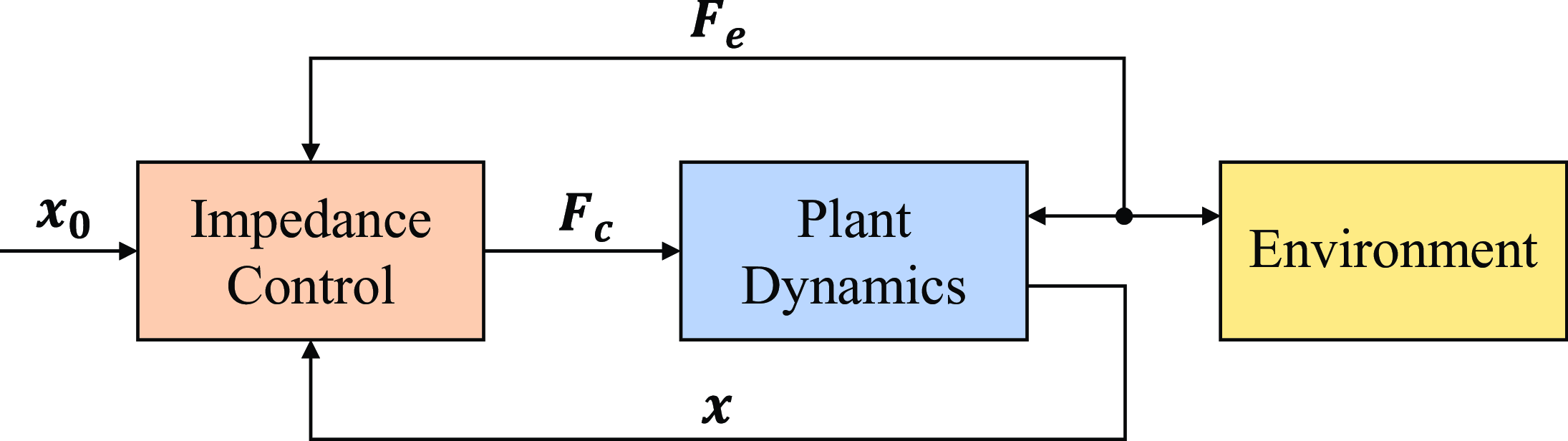
Figure 3. Diagram of impedance control.
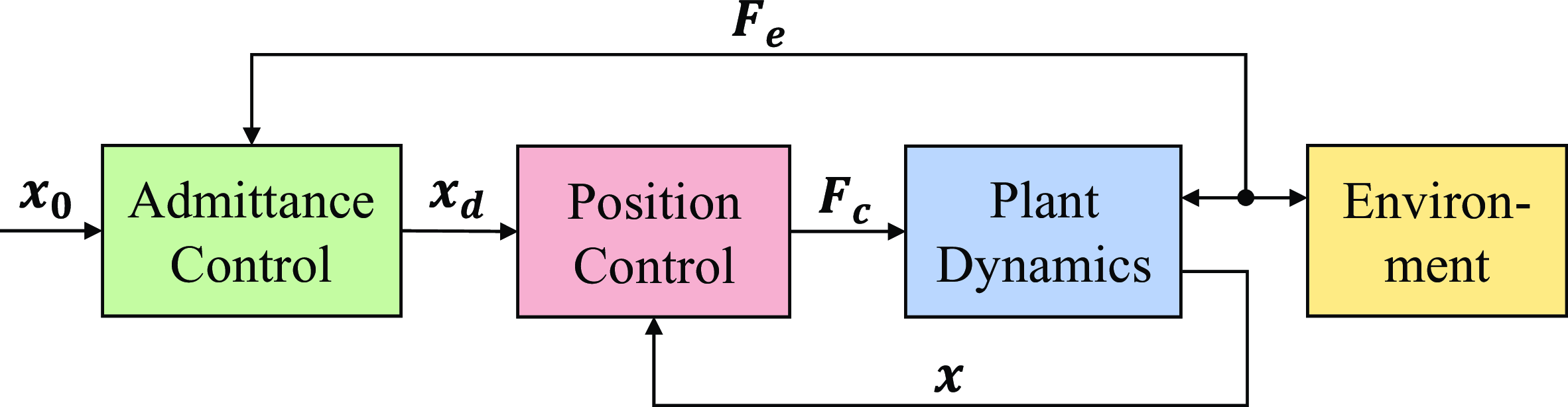
Figure 4. Diagram of admittance control.
Remark 1. As a second-order system, the mass–spring–damper model can describe a wider range of environments than the damper–spring model. For example, (6) can describe the environment dynamics in human–robot interaction. To simplify the analysis, the environmental inertia, damping, and stiffness are assumed to be fixed.
2.2. Impedance control and admittance control
Impedance control and admittance control are two complementary implementations of regulating the mechanical impedance of manipulators to the target impedance model described by:
 \begin{equation} \boldsymbol{F}_{\boldsymbol{e}}=f(\boldsymbol{x},\boldsymbol{x}_{\textbf{0}}) \end{equation}
where
 $\boldsymbol{x}_{\textbf{0}}$
is the virtual equilibrium trajectory and
$\boldsymbol{x}_{\textbf{0}}$
is the virtual equilibrium trajectory and
 $f({\cdot})$
is a target impedance function. Equation (7) is a general impedance model which describes a dynamical relationship between the motion and the contact force. In this article, we adopt the impedance model
$f({\cdot})$
is a target impedance function. Equation (7) is a general impedance model which describes a dynamical relationship between the motion and the contact force. In this article, we adopt the impedance model
 $\boldsymbol{F}_{\boldsymbol{e}}=\boldsymbol{H}_{\boldsymbol{d}}\ddot{\boldsymbol{x}}+\boldsymbol{C}_{\boldsymbol{d}}\dot{\boldsymbol{x}}+\boldsymbol{K}_{\boldsymbol{d}}\boldsymbol{x}-\boldsymbol{K}^{\prime}_{\boldsymbol{d}}\boldsymbol{x}_{\textbf{0}}$
as the target, where
$\boldsymbol{F}_{\boldsymbol{e}}=\boldsymbol{H}_{\boldsymbol{d}}\ddot{\boldsymbol{x}}+\boldsymbol{C}_{\boldsymbol{d}}\dot{\boldsymbol{x}}+\boldsymbol{K}_{\boldsymbol{d}}\boldsymbol{x}-\boldsymbol{K}^{\prime}_{\boldsymbol{d}}\boldsymbol{x}_{\textbf{0}}$
as the target, where
 $\boldsymbol{H}_{\boldsymbol{d}}$
,
$\boldsymbol{H}_{\boldsymbol{d}}$
,
 $\boldsymbol{C}_{\boldsymbol{d}}$
,
$\boldsymbol{C}_{\boldsymbol{d}}$
,
 $\boldsymbol{K}_{\boldsymbol{d}}$
, and
$\boldsymbol{K}_{\boldsymbol{d}}$
, and
 $\boldsymbol{K}^{\prime}_{\boldsymbol{d}}$
are the desired inertia, damping, stiffness, and auxiliary stiffness matrices, respectively.
$\boldsymbol{K}^{\prime}_{\boldsymbol{d}}$
are the desired inertia, damping, stiffness, and auxiliary stiffness matrices, respectively.
In impedance control, as the controlled plant, robot dynamics (5) acts as an admittance, so the controller is designed as an impedance accordingly. The control force
 ${\boldsymbol{F}}_{\boldsymbol{c}}$
is designed to eliminate the difference between the robot dynamics and the target impedance model directly. While in admittance control, an outer loop controller and an inner loop controller need to be designed. The outer loop controller generates the desired trajectory
${\boldsymbol{F}}_{\boldsymbol{c}}$
is designed to eliminate the difference between the robot dynamics and the target impedance model directly. While in admittance control, an outer loop controller and an inner loop controller need to be designed. The outer loop controller generates the desired trajectory
 $\boldsymbol{x}_{\boldsymbol{d}}$
that satisfies the desired interaction behavior. By replacing
$\boldsymbol{x}_{\boldsymbol{d}}$
that satisfies the desired interaction behavior. By replacing
 $\boldsymbol{x}$
with
$\boldsymbol{x}$
with
 $\boldsymbol{x}_{\boldsymbol{d}}$
in (7), the form of the outer loop controller becomes
$\boldsymbol{x}_{\boldsymbol{d}}$
in (7), the form of the outer loop controller becomes
 $\boldsymbol{F}_{\boldsymbol{e}}=f(\boldsymbol{x}_{\boldsymbol{d}},\boldsymbol{x}_{\textbf{0}})$
. The inner loop controller ensures trajectory tracking, that is,
$\boldsymbol{F}_{\boldsymbol{e}}=f(\boldsymbol{x}_{\boldsymbol{d}},\boldsymbol{x}_{\textbf{0}})$
. The inner loop controller ensures trajectory tracking, that is,
 $\lim _{t\to \infty }\boldsymbol{x}(t)=\boldsymbol{x}_{\boldsymbol{d}}(t)$
. On the contrary, admittance control regards the position-controlled system including the inner loop controller as the controlled plant, which acts as an impedance, so the outer loop controller is designed as an admittance. The diagrams of these two controllers are illustrated in Fig. 3 and Fig. 4, respectively.
$\lim _{t\to \infty }\boldsymbol{x}(t)=\boldsymbol{x}_{\boldsymbol{d}}(t)$
. On the contrary, admittance control regards the position-controlled system including the inner loop controller as the controlled plant, which acts as an impedance, so the outer loop controller is designed as an admittance. The diagrams of these two controllers are illustrated in Fig. 3 and Fig. 4, respectively.
2.3. LQR
Consider a continuous linear time-invariant system described by:
 \begin{equation} \dot{\boldsymbol{\xi }}=\boldsymbol{A}\boldsymbol{\xi }+\boldsymbol{B}\boldsymbol{u} \end{equation}
where
 $\boldsymbol{\xi }\in \mathbb{R}^m$
and
$\boldsymbol{\xi }\in \mathbb{R}^m$
and
 $\boldsymbol{u}\in \mathbb{R}^r$
denote the system state and input, respectively.
$\boldsymbol{u}\in \mathbb{R}^r$
denote the system state and input, respectively.
 $\boldsymbol{A}\in \mathbb{R}^{m\times{m}}$
and
$\boldsymbol{A}\in \mathbb{R}^{m\times{m}}$
and
 $\boldsymbol{B}\in \mathbb{R}^{m\times{r}}$
denote the system matrix and input matrix, respectively. The goal is to design the optimal control input:
$\boldsymbol{B}\in \mathbb{R}^{m\times{r}}$
denote the system matrix and input matrix, respectively. The goal is to design the optimal control input:
 \begin{equation} \boldsymbol{u}=-{\boldsymbol{K}}\boldsymbol{\xi } \end{equation}
to minimize the cost function:
 \begin{equation} J=\int _{0}^{\infty }\!\left(\boldsymbol{\xi }^T{\boldsymbol{Q}}\boldsymbol{\xi }+\boldsymbol{u}^T\boldsymbol{R}\boldsymbol{u}\right)\!dt \end{equation}
where
 ${\boldsymbol{Q}}\in \mathbb{R}^{m\times{m}}$
and
${\boldsymbol{Q}}\in \mathbb{R}^{m\times{m}}$
and
 $\boldsymbol{R}\in \mathbb{R}^{r\times{r}}$
denote the weights of system state and input satisfying
$\boldsymbol{R}\in \mathbb{R}^{r\times{r}}$
denote the weights of system state and input satisfying
 ${\boldsymbol{Q}}={\boldsymbol{Q}}^T\geq{\textbf{0}}$
and
${\boldsymbol{Q}}={\boldsymbol{Q}}^T\geq{\textbf{0}}$
and
 $\boldsymbol{R}=\boldsymbol{R}^T\gt \textbf{0}$
. By solving the algebraic Riccati equation (ARE) using known
$\boldsymbol{R}=\boldsymbol{R}^T\gt \textbf{0}$
. By solving the algebraic Riccati equation (ARE) using known
 $\boldsymbol{A}$
and
$\boldsymbol{A}$
and
 $\boldsymbol{B}$
, the unique symmetric positive definite matrix
$\boldsymbol{B}$
, the unique symmetric positive definite matrix
 ${\boldsymbol{Y}}^*$
can be obtained [Reference Lewis, Vrabie and Syrmos21]:
${\boldsymbol{Y}}^*$
can be obtained [Reference Lewis, Vrabie and Syrmos21]:
 \begin{equation} {\boldsymbol{Y}}\boldsymbol{A}+\boldsymbol{A}^T{\boldsymbol{Y}}+{\boldsymbol{Q}}-{\boldsymbol{Y}}\boldsymbol{B}\boldsymbol{R}^{-1}\boldsymbol{B}^T{\boldsymbol{Y}}=\textbf{0}. \end{equation}
Then, we can calculate the optimal feedback gain
 ${\boldsymbol{K}}^*$
in (9):
${\boldsymbol{K}}^*$
in (9):
 \begin{equation} {\boldsymbol{K}}^*=\boldsymbol{R}^{-1}\boldsymbol{B}^T{\boldsymbol{Y}}^*. \end{equation}
3. Methodology
In this section, the HIAC scheme under the second-order unknown environment is illustrated, which can be divided into the impedance iteration stage and optimal implementation stage, as shown in Fig. 5. In the impedance iteration stage, the target impedance model is adjusted iteratively by the proposed impedance adaptation method to minimize the cost function. In the optimal implementation stage, the obtained target impedance model is implemented optimally by the proposed hybrid system framework with the mapping of the optimal duty cycle.

Figure 5. Diagram of HIAC scheme.
3.1. Adaptive optimal control
In this section, an adaptive optimal control method is to solve the optimal feedback gain that minimizes the cost function (10) when
 $\boldsymbol{A}$
and
$\boldsymbol{A}$
and
 $\boldsymbol{B}$
in the system (8) are unknown constant matrices [Reference Jiang and Jiang23]. The required definitions are first imported as:
$\boldsymbol{B}$
in the system (8) are unknown constant matrices [Reference Jiang and Jiang23]. The required definitions are first imported as:
 \begin{align} \hat{{\boldsymbol{Y}}}&=[Y_{11},2Y_{12},\cdots,2Y_{1m},Y_{22},2Y_{23},\cdots,Y_{mm}]^T \notag \\[3pt] \bar{\boldsymbol{\xi }}&=\bigl [\xi _1^2,\xi _1\xi _2,\cdots,\xi _1\xi _m,\xi _2^2,\xi _2\xi _3,\cdots,\xi _m^2\bigr ]^T \notag \\[3pt] \boldsymbol{\delta _{\xi \xi }}&=\bigl [\bar{\boldsymbol{\xi }}(t_1)-\bar{\boldsymbol{\xi }}(t_0),\bar{\boldsymbol{\xi }}(t_2)-\bar{\boldsymbol{\xi }}(t_1),\cdots,\bar{\boldsymbol{\xi }}(t_l)-\bar{\boldsymbol{\xi }}(t_{l-1})\bigr ]^T \notag \\[3pt] \boldsymbol{I}_{\boldsymbol{\xi \xi}}&=\biggl [\int _{t_0}^{t_1}\boldsymbol{\xi }\otimes \boldsymbol{\xi }dt,\int _{t_1}^{t_2}\boldsymbol{\xi }\otimes \boldsymbol{\xi }dt,\cdots,\int _{t_{l-1}}^{t_l}\boldsymbol{\xi }\otimes \boldsymbol{\xi }dt\biggr ]^T \notag \\[3pt] \boldsymbol{I}_{\boldsymbol{\xi}\boldsymbol{u}}&=\biggl [\int _{t_0}^{t_1}\boldsymbol{\xi }\otimes \boldsymbol{u}dt,\int _{t_1}^{t_2}\boldsymbol{\xi }\otimes \boldsymbol{u}dt,\cdots,\int _{t_{l-1}}^{t_l}\boldsymbol{\xi }\otimes \boldsymbol{u}dt\biggr ]^T \end{align}
where
 $0\leq{t_0}\lt t_1\lt \cdots \lt t_l$
,
$0\leq{t_0}\lt t_1\lt \cdots \lt t_l$
,
 ${\boldsymbol{Y}}\in \mathbb{R}^{m\times{m}}\to \hat{{\boldsymbol{Y}}}\in \mathbb{R}^{\frac{1}{2}m(m+1)}$
,
${\boldsymbol{Y}}\in \mathbb{R}^{m\times{m}}\to \hat{{\boldsymbol{Y}}}\in \mathbb{R}^{\frac{1}{2}m(m+1)}$
,
 $\boldsymbol{\xi }\in \mathbb{R}^m\to \bar{\boldsymbol{\xi }}\in \mathbb{R}^{\frac{1}{2}m(m+1)}$
,
$\boldsymbol{\xi }\in \mathbb{R}^m\to \bar{\boldsymbol{\xi }}\in \mathbb{R}^{\frac{1}{2}m(m+1)}$
,
 $\boldsymbol{\delta _{\xi \xi }}\in \mathbb{R}^{l\times{\frac{1}{2}m(m+1)}}$
,
$\boldsymbol{\delta _{\xi \xi }}\in \mathbb{R}^{l\times{\frac{1}{2}m(m+1)}}$
,
 $\boldsymbol{I}_{\boldsymbol{\xi \xi}}\in \mathbb{R}^{l\times{m^2}}$
,
$\boldsymbol{I}_{\boldsymbol{\xi \xi}}\in \mathbb{R}^{l\times{m^2}}$
,
 $\boldsymbol{I}_{\boldsymbol{\xi}\boldsymbol{u}}\in \mathbb{R}^{l\times{mr}}$
,
$\boldsymbol{I}_{\boldsymbol{\xi}\boldsymbol{u}}\in \mathbb{R}^{l\times{mr}}$
,
 $P_{ij}$
and
$P_{ij}$
and
 $\xi _{i}$
denote the elements of
$\xi _{i}$
denote the elements of
 ${\boldsymbol{Y}}$
and
${\boldsymbol{Y}}$
and
 $\boldsymbol{\xi }$
, respectively,
$\boldsymbol{\xi }$
, respectively,
 $l$
is the sampling times, and
$l$
is the sampling times, and
 $\otimes$
is the Kronecker product.
$\otimes$
is the Kronecker product.
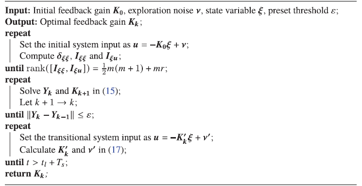
The initial system input of time interval
 $t\in [t_0,t_l]$
is designed as
$t\in [t_0,t_l]$
is designed as
 $\boldsymbol{u}=-\boldsymbol{K}_{\textbf{0}}\boldsymbol{\xi }+\boldsymbol{\nu }$
, where
$\boldsymbol{u}=-\boldsymbol{K}_{\textbf{0}}\boldsymbol{\xi }+\boldsymbol{\nu }$
, where
 $\boldsymbol{K}_{\textbf{0}}$
is the initial feedback gain to stabilize the system and
$\boldsymbol{K}_{\textbf{0}}$
is the initial feedback gain to stabilize the system and
 $\boldsymbol{\nu }$
is the exploration noise to make the system satisfy the persistent excitation (PE) condition. The matrices
$\boldsymbol{\nu }$
is the exploration noise to make the system satisfy the persistent excitation (PE) condition. The matrices
 $\boldsymbol{\delta _{\xi \xi }}$
,
$\boldsymbol{\delta _{\xi \xi }}$
,
 $\boldsymbol{I}_{\boldsymbol{\xi \xi}}$
, and
$\boldsymbol{I}_{\boldsymbol{\xi \xi}}$
, and
 $\boldsymbol{I}_{\boldsymbol{\xi}\boldsymbol{u}}$
defined above are computed until the rank condition is satisfied:
$\boldsymbol{I}_{\boldsymbol{\xi}\boldsymbol{u}}$
defined above are computed until the rank condition is satisfied:
 \begin{equation} \textrm{rank}\!\left([\boldsymbol{I}_{\boldsymbol{\xi \xi}},\boldsymbol{I}_{\boldsymbol{\xi}\boldsymbol{u}}]\right)=\frac{1}{2}m(m+1)+mr. \end{equation}
When the sampling times
 $l$
is large enough and the rank condition (14) is satisfied,
$l$
is large enough and the rank condition (14) is satisfied,
 $\boldsymbol{Y}_{\boldsymbol{k}}$
and
$\boldsymbol{Y}_{\boldsymbol{k}}$
and
 $\boldsymbol{K}_{\boldsymbol{k} \textbf{+} \textbf{1}}$
can be computed iteratively by:
$\boldsymbol{K}_{\boldsymbol{k} \textbf{+} \textbf{1}}$
can be computed iteratively by:
 \begin{equation} \begin{bmatrix} \hat{\boldsymbol{Y}}_{\boldsymbol{k}} \\[3pt] \textrm{vec}\!\left(\boldsymbol{K}_{\boldsymbol{k} \textbf{+} \textbf{1}}\right) \end{bmatrix} = \left(\boldsymbol{\Theta}_{\boldsymbol{k}}^T\boldsymbol{\Theta}_{\boldsymbol{k}}\right)^{-1}\boldsymbol{\Theta}_{\boldsymbol{k}}^T\boldsymbol{\Xi}_{\boldsymbol{k}} \end{equation}
where
 $k$
is the number of iterations.
$k$
is the number of iterations.
 $\boldsymbol{\Theta}_{\boldsymbol{k}}$
and
$\boldsymbol{\Theta}_{\boldsymbol{k}}$
and
 $\boldsymbol{\Xi}_{\boldsymbol{k}}$
are defined as:
$\boldsymbol{\Xi}_{\boldsymbol{k}}$
are defined as:
 \begin{align} \boldsymbol{\Theta}_{\boldsymbol{k}}&=\left[\boldsymbol{\delta _{\xi \xi }},-2\boldsymbol{I}_{\boldsymbol{\xi \xi}}\!\left(\boldsymbol{I}_{\boldsymbol{m}}\otimes \boldsymbol{K}_{\boldsymbol{k}}^T\boldsymbol{R}\right)-2\boldsymbol{I}_{\boldsymbol{\xi}\boldsymbol{u}}(\boldsymbol{I}_{\boldsymbol{m}}\otimes \boldsymbol{R})\right] \notag \\[5pt] \boldsymbol{\Xi}_{\boldsymbol{k}}&=-\boldsymbol{I}_{\boldsymbol{\xi \xi}}\textrm{vec}\!\left({\boldsymbol{Q}}+\boldsymbol{K}_{\boldsymbol{k}}^T\boldsymbol{R}\boldsymbol{K}_{\boldsymbol{k}}\right) \end{align}
where
 $\boldsymbol{I}_{\boldsymbol{m}}\in \mathbb{R}^{m\times{m}}$
is an identity matrix and
$\boldsymbol{I}_{\boldsymbol{m}}\in \mathbb{R}^{m\times{m}}$
is an identity matrix and
 $\textrm{vec}({\cdot})$
is the function that stretches a matrix into a vector. Let
$\textrm{vec}({\cdot})$
is the function that stretches a matrix into a vector. Let
 $k+1\to{k}$
and repeat the above calculation until
$k+1\to{k}$
and repeat the above calculation until
 $\Vert{\boldsymbol{Y}_{\boldsymbol{k}}}-\boldsymbol{Y}_{\boldsymbol{k}-\textbf{1}}\Vert \leq \varepsilon$
where
$\Vert{\boldsymbol{Y}_{\boldsymbol{k}}}-\boldsymbol{Y}_{\boldsymbol{k}-\textbf{1}}\Vert \leq \varepsilon$
where
 $\varepsilon \gt 0$
is a preset threshold, and the optimal feedback gain
$\varepsilon \gt 0$
is a preset threshold, and the optimal feedback gain
 $\boldsymbol{K}_{\boldsymbol{k}}$
is obtained. To proceed, we design smooth functions for the feedback gain and the exploration noise to keep the system input continuous [Reference Huang, Yang and Chen25]:
$\boldsymbol{K}_{\boldsymbol{k}}$
is obtained. To proceed, we design smooth functions for the feedback gain and the exploration noise to keep the system input continuous [Reference Huang, Yang and Chen25]:
 \begin{align} \boldsymbol{K}^{\prime}_{\boldsymbol{k}}&=\frac{\boldsymbol{K}_{\boldsymbol{k}}+\boldsymbol{K}_{\textbf{0}}}{2}+\frac{\boldsymbol{K}_{\boldsymbol{k}}-\boldsymbol{K}_{\textbf{0}}}{2}\sin \!\left(-\frac{\pi }{2}+\frac{t-t_l}{T_s}\pi \right) \notag \\[5pt] \boldsymbol{\nu}^{\prime}&=\frac{\boldsymbol{\nu }(t_l)}{2}-\frac{\boldsymbol{\nu }(t_l)}{2}\sin \!\left(-\frac{\pi }{2}+\frac{t-t_l}{T_s}\pi \right) \end{align}
where
 $\boldsymbol{K}^{\prime}_{\boldsymbol{k}}$
is the transitional feedback gain,
$\boldsymbol{K}^{\prime}_{\boldsymbol{k}}$
is the transitional feedback gain,
 $\boldsymbol{\nu}^{\prime}$
is the transitional exploration noise,
$\boldsymbol{\nu}^{\prime}$
is the transitional exploration noise,
 $\boldsymbol{\nu }(t_l)$
is the value of
$\boldsymbol{\nu }(t_l)$
is the value of
 $\boldsymbol{\nu }$
at time
$\boldsymbol{\nu }$
at time
 $t_l$
, and
$t_l$
, and
 $T_s$
is the transitional time. The transitional system input is designed as
$T_s$
is the transitional time. The transitional system input is designed as
 $\boldsymbol{u}=-\boldsymbol{K}^{\prime}_{\boldsymbol{k}}\boldsymbol{\xi }+\boldsymbol{\nu}^{\prime}$
in time interval
$\boldsymbol{u}=-\boldsymbol{K}^{\prime}_{\boldsymbol{k}}\boldsymbol{\xi }+\boldsymbol{\nu}^{\prime}$
in time interval
 $t_l\lt t\leq{t}_l+T_s$
during which
$t_l\lt t\leq{t}_l+T_s$
during which
 $\boldsymbol{K}^{\prime}_{\boldsymbol{k}}$
changes from
$\boldsymbol{K}^{\prime}_{\boldsymbol{k}}$
changes from
 $\boldsymbol{K}_{\textbf{0}}$
to
$\boldsymbol{K}_{\textbf{0}}$
to
 $\boldsymbol{K}_{\boldsymbol{k}}$
and
$\boldsymbol{K}_{\boldsymbol{k}}$
and
 $\boldsymbol{\nu}^{\prime}$
changes from
$\boldsymbol{\nu}^{\prime}$
changes from
 $\boldsymbol{\nu }(t_l)$
to
$\boldsymbol{\nu }(t_l)$
to
 $\textbf{0}$
smoothly. When
$\textbf{0}$
smoothly. When
 $t\gt t_l+T_s$
, the system input becomes
$t\gt t_l+T_s$
, the system input becomes
 $\boldsymbol{u}=-\boldsymbol{K}_{\boldsymbol{k}}\boldsymbol{\xi }$
. The principle of the above algorithm is summarized in Algorithm 1.
$\boldsymbol{u}=-\boldsymbol{K}_{\boldsymbol{k}}\boldsymbol{\xi }$
. The principle of the above algorithm is summarized in Algorithm 1.
Algorithm 1 Adaptive Optimal Control
3.2. Impedance adaptation
In this section, we propose a novel impedance adaptation method to obtain the optimal second-order target impedance model in the second-order unknown environment. Assume that the manipulator is interacting with a virtual environment that consists of two parts, one is the mass–spring–damper system described in (6) and the other is the virtual inertia denoted as
 $\boldsymbol{H}_{\boldsymbol{d}}$
, which is realized by defining the virtual interaction force
$\boldsymbol{H}_{\boldsymbol{d}}$
, which is realized by defining the virtual interaction force
 $\boldsymbol{F}_{\boldsymbol{ev}}$
as:
$\boldsymbol{F}_{\boldsymbol{ev}}$
as:
 \begin{equation} \boldsymbol{F}_{\boldsymbol{ev}}=\boldsymbol{F}_{\boldsymbol{e}}-\boldsymbol{H}_{\boldsymbol{d}}\ddot{\boldsymbol{x}}. \end{equation}
Substituting (18) into (6), we have
 \begin{equation} \boldsymbol{H}_{\boldsymbol{t}}\ddot{\boldsymbol{x}}+\boldsymbol{C}_{\boldsymbol{m}}\dot{\boldsymbol{x}}+\boldsymbol{G}_{\boldsymbol{m}}\boldsymbol{x}=-\boldsymbol{F}_{\boldsymbol{ev}} \end{equation}
where
 $\boldsymbol{H}_{\boldsymbol{t}}=\boldsymbol{H}_{\boldsymbol{m}}+\boldsymbol{H}_{\boldsymbol{d}}$
denotes the total inertia of the virtual environment. Compare (8) with (19), we need to rewrite (19) as a linear time-invariant system [Reference Ge, Li and Wang24]:
$\boldsymbol{H}_{\boldsymbol{t}}=\boldsymbol{H}_{\boldsymbol{m}}+\boldsymbol{H}_{\boldsymbol{d}}$
denotes the total inertia of the virtual environment. Compare (8) with (19), we need to rewrite (19) as a linear time-invariant system [Reference Ge, Li and Wang24]:
 \begin{equation} \dot{\boldsymbol{\xi }}=\boldsymbol{A}\boldsymbol{\xi }+\boldsymbol{B}\boldsymbol{F}_{\boldsymbol{ev}} \end{equation}
where
 $\boldsymbol{\xi }=[\dot{\boldsymbol{x}}^T,\boldsymbol{x}^T,\boldsymbol{z}^T]^T$
is the system state and
$\boldsymbol{\xi }=[\dot{\boldsymbol{x}}^T,\boldsymbol{x}^T,\boldsymbol{z}^T]^T$
is the system state and
 $\boldsymbol{z}\in \mathbb{R}^p$
is generated by:
$\boldsymbol{z}\in \mathbb{R}^p$
is generated by:
 \begin{equation} \begin{cases} \dot{\boldsymbol{z}}=\boldsymbol{U}\boldsymbol{z} \\ \boldsymbol{x}_{\textbf{0}}=\boldsymbol{V}\boldsymbol{z} \end{cases} \end{equation}
where
 $\boldsymbol{U}\in \mathbb{R}^{p\times{p}}$
and
$\boldsymbol{U}\in \mathbb{R}^{p\times{p}}$
and
 $\boldsymbol{V}\in \mathbb{R}^{n\times{p}}$
are two predefined matrices. Then, we have
$\boldsymbol{V}\in \mathbb{R}^{n\times{p}}$
are two predefined matrices. Then, we have
 \begin{equation} \boldsymbol{A}=\begin{bmatrix} -\boldsymbol{H}_{\boldsymbol{t}}^{-1}\boldsymbol{C}_{\boldsymbol{m}} & \quad -\boldsymbol{H}_{\boldsymbol{t}}^{-1}\boldsymbol{G}_{\boldsymbol{m}} & \quad \textbf{0} \\[4pt] \boldsymbol{I}_{\boldsymbol{n}} & \quad \textbf{0} & \quad \textbf{0} \\[4pt] \textbf{0} & \quad \textbf{0} & \quad \boldsymbol{U} \end{bmatrix},\boldsymbol{B}=\begin{bmatrix} -\boldsymbol{H}_{\boldsymbol{t}}^{-1} \\[4pt] \textbf{0} \\[4pt] \textbf{0} \end{bmatrix} \end{equation}
where
 $\boldsymbol{A}$
and
$\boldsymbol{A}$
and
 $\boldsymbol{B}$
are unknown due to the unknown environment dynamics. A cost function that represents the trade-off between trajectory tracking and force regulation is defined as:
$\boldsymbol{B}$
are unknown due to the unknown environment dynamics. A cost function that represents the trade-off between trajectory tracking and force regulation is defined as:
 \begin{equation} J_1=\int _0^{\infty }\left[\dot{\boldsymbol{x}}^T\boldsymbol{Q}_{\textbf{1}}\dot{\boldsymbol{x}}+(\boldsymbol{x}-\boldsymbol{x}_{\textbf{0}})^T\boldsymbol{Q}_{\textbf{2}}(\boldsymbol{x}-\boldsymbol{x}_{\textbf{0}})+\boldsymbol{F}_{\boldsymbol{ev}}^T\boldsymbol{R}\boldsymbol{F}_{\boldsymbol{ev}}\right]\!dt \end{equation}
where
 $\boldsymbol{Q}_{\textbf{1}},\boldsymbol{Q}_{\textbf{2}}\in \mathbb{R}^{n\times{n}}$
are the weights of tracking error and
$\boldsymbol{Q}_{\textbf{1}},\boldsymbol{Q}_{\textbf{2}}\in \mathbb{R}^{n\times{n}}$
are the weights of tracking error and
 $\boldsymbol{R}\in \mathbb{R}^{n\times{n}}$
is the weight of the virtual interaction force. According to the states defined above, (23) can be rewritten as:
$\boldsymbol{R}\in \mathbb{R}^{n\times{n}}$
is the weight of the virtual interaction force. According to the states defined above, (23) can be rewritten as:
 \begin{equation} J_1=\int _0^{\infty }\left(\boldsymbol{\xi }^T{\boldsymbol{Q}}\boldsymbol{\xi }+\boldsymbol{F}_{\boldsymbol{ev}}^T\boldsymbol{R}\boldsymbol{F}_{\boldsymbol{ev}}\right)\!dt \end{equation}
where
 \begin{equation*} {\boldsymbol{Q}}=\begin {bmatrix} {\boldsymbol{Q}}_{\textbf{1}} & \quad \textbf{0} & \quad \textbf{0} \\[5pt] \textbf{0} & \quad {\boldsymbol{Q}}_{\textbf{2}} & \quad -{\boldsymbol{Q}}_{\textbf{2}}{\boldsymbol{V}} \\[5pt] \textbf{0} & \quad -{\boldsymbol{V}}^T{\boldsymbol{Q}}_{\textbf{2}} & \quad {\boldsymbol{V}}^T{\boldsymbol{Q}}_{\textbf{2}}{\boldsymbol{V}} \end {bmatrix}. \end{equation*}
Therefore, the cost function (24) can be minimized by regarding the virtual interaction force
 $\boldsymbol{F}_{\boldsymbol{ev}}$
in (20) as the system input:
$\boldsymbol{F}_{\boldsymbol{ev}}$
in (20) as the system input:
 \begin{equation} \boldsymbol{F}_{\boldsymbol{ev}}=-\boldsymbol{K}_{\boldsymbol{k}}\boldsymbol{\xi } \end{equation}
where
 $\boldsymbol{K}_{\boldsymbol{k}}=[\boldsymbol{K}_{\boldsymbol{k}1},\boldsymbol{K}_{\boldsymbol{k}2},\boldsymbol{K}_{\boldsymbol{k}3}]$
is obtained according to Algorithm 1 with
$\boldsymbol{K}_{\boldsymbol{k}}=[\boldsymbol{K}_{\boldsymbol{k}1},\boldsymbol{K}_{\boldsymbol{k}2},\boldsymbol{K}_{\boldsymbol{k}3}]$
is obtained according to Algorithm 1 with
 $\boldsymbol{K}_{\boldsymbol{k}1},\boldsymbol{K}_{\boldsymbol{k}2}\in \mathbb{R}^{n\times{n}}$
and
$\boldsymbol{K}_{\boldsymbol{k}1},\boldsymbol{K}_{\boldsymbol{k}2}\in \mathbb{R}^{n\times{n}}$
and
 $\boldsymbol{K}_{\boldsymbol{k}3}\in \mathbb{R}^{n\times{p}}$
. Substituting (18) and (21) into (25), we have
$\boldsymbol{K}_{\boldsymbol{k}3}\in \mathbb{R}^{n\times{p}}$
. Substituting (18) and (21) into (25), we have
 \begin{equation} \boldsymbol{F}_{\boldsymbol{e}}=\boldsymbol{H}_{\boldsymbol{d}}\ddot{\boldsymbol{x}}-\boldsymbol{K}_{\boldsymbol{k}1}\dot{\boldsymbol{x}}-\boldsymbol{K}_{\boldsymbol{k}2}\boldsymbol{x}-\boldsymbol{K}_{\boldsymbol{k}3}\left(\boldsymbol{V}^T\boldsymbol{V}\right)^{-1}\boldsymbol{V}^T\boldsymbol{x}_{\textbf{0}}. \end{equation}
Comparing (26) with (7), we can rewrite (26) as:
 \begin{equation} \boldsymbol{F}_{\boldsymbol{e}}=\boldsymbol{H}_{\boldsymbol{d}}\ddot{\boldsymbol{x}}+\boldsymbol{C}_{\boldsymbol{d}}\dot{\boldsymbol{x}}+\boldsymbol{K}_{\boldsymbol{d}}\boldsymbol{x}-\boldsymbol{K}^{\prime}_{\boldsymbol{d}}\boldsymbol{x}_{\textbf{0}}. \end{equation}
Note that (27) denotes the target impedance model equivalent to the system input (25) with
 $\boldsymbol{C}_{\boldsymbol{d}}=-\boldsymbol{K}_{\boldsymbol{k}1}$
,
$\boldsymbol{C}_{\boldsymbol{d}}=-\boldsymbol{K}_{\boldsymbol{k}1}$
,
 $\boldsymbol{K}_{\boldsymbol{d}}=-\boldsymbol{K}_{\boldsymbol{k}2}$
and
$\boldsymbol{K}_{\boldsymbol{d}}=-\boldsymbol{K}_{\boldsymbol{k}2}$
and
 $\boldsymbol{K}^{\prime}_{\boldsymbol{d}}=\boldsymbol{K}_{\boldsymbol{k}3}(\boldsymbol{V}^T\boldsymbol{V})^{-1}\boldsymbol{V}^T$
. So the target impedance model representing the optimal interaction behavior is obtained from the interaction dynamics of the robot and the second-order unknown environment, and the model is second order due to the introduced virtual inertia
$\boldsymbol{K}^{\prime}_{\boldsymbol{d}}=\boldsymbol{K}_{\boldsymbol{k}3}(\boldsymbol{V}^T\boldsymbol{V})^{-1}\boldsymbol{V}^T$
. So the target impedance model representing the optimal interaction behavior is obtained from the interaction dynamics of the robot and the second-order unknown environment, and the model is second order due to the introduced virtual inertia
 $\boldsymbol{H}_{\boldsymbol{d}}$
.
$\boldsymbol{H}_{\boldsymbol{d}}$
.
Remark 2. It can be seen from (25) that the virtual inertia eliminates the acceleration term in the system input. In addition, the system input in Algorithm 1 is realized by implementing the equivalent second-order impedance model using impedance control without acceleration feedback. Hence, the proposed method does not require acceleration feedback which is difficult to obtain in practice and can adapt to a wider range of environments than the approach in ref. [Reference Ge, Li and Wang24].
3.3. Hybrid system framework
In this section, we design a novel hybrid system framework to implement the target impedance model in the second-order environment. An overview of the proposed framework is shown in Fig. 6. First, the well-known computed torque control method is utilized to design the control law [Reference Slotine and Li33]. For impedance control, the control law is designed in Cartesian space as:
 \begin{equation} {\boldsymbol{F}}_{\boldsymbol{ci}}={\boldsymbol{H}}_{\boldsymbol{x}}(\boldsymbol{q}){\boldsymbol{v}}_{\boldsymbol{ci}}+{\boldsymbol{C}}_{\boldsymbol{x}}(\boldsymbol{q},\dot{\boldsymbol{q}})\dot{\boldsymbol{x}}+{\boldsymbol{G}}_{\boldsymbol{x}}(\boldsymbol{q})-\boldsymbol{F}_{\boldsymbol{e}} \end{equation}
where
 ${\boldsymbol{F}}_{\boldsymbol{ci}}$
and
${\boldsymbol{F}}_{\boldsymbol{ci}}$
and
 ${\boldsymbol{v}}_{\boldsymbol{ci}}$
are the control force and the equivalent input of impedance control, respectively. Substituting (28) into (5), yields
${\boldsymbol{v}}_{\boldsymbol{ci}}$
are the control force and the equivalent input of impedance control, respectively. Substituting (28) into (5), yields

Figure 6. Diagram of hybrid system framework.
 \begin{equation} \ddot{\boldsymbol{x}}={\boldsymbol{v}}_{\boldsymbol{ci}}. \end{equation}
Substituting (29) into (27), we have
 \begin{equation} {\boldsymbol{v}}_{\boldsymbol{ci}}=\boldsymbol{H}_{\boldsymbol{d}}^{-1}\!\left(\boldsymbol{F}_{\boldsymbol{e}}-\boldsymbol{C}_{\boldsymbol{d}}\dot{\boldsymbol{x}}-\boldsymbol{K}_{\boldsymbol{d}}\boldsymbol{x}+\boldsymbol{K}^{\prime}_{\boldsymbol{d}}\boldsymbol{x}_{\textbf{0}}\right). \end{equation}
It can be seen that impedance control uses interaction force feedback instead of acceleration feedback due to the second-order inertia term in (27). For admittance control, replacing
 $\boldsymbol{x}$
in (27) with the desired trajectory
$\boldsymbol{x}$
in (27) with the desired trajectory
 $\boldsymbol{x}_{\boldsymbol{d}}$
, the update law of
$\boldsymbol{x}_{\boldsymbol{d}}$
, the update law of
 $\boldsymbol{x}_{\boldsymbol{d}}$
in the outer loop controller is obtained as:
$\boldsymbol{x}_{\boldsymbol{d}}$
in the outer loop controller is obtained as:
 \begin{equation} \boldsymbol{H}_{\boldsymbol{d}}\ddot{\boldsymbol{x}}_\boldsymbol{d}+\boldsymbol{C}_{\boldsymbol{d}}\dot{\boldsymbol{x}}_\boldsymbol{d}+\boldsymbol{K}_{\boldsymbol{d}}\boldsymbol{x}_{\boldsymbol{d}}-\boldsymbol{K}^{\prime}_{\boldsymbol{d}}\boldsymbol{x}_{\textbf{0}}=\boldsymbol{F}_{\boldsymbol{e}}. \end{equation}
The inner loop controller is designed as:
 \begin{equation} {\boldsymbol{F}}_{\boldsymbol{ca}}={\boldsymbol{H}}_{\boldsymbol{x}}(\boldsymbol{q}){\boldsymbol{v}}_{\boldsymbol{ca}}+{\boldsymbol{C}}_{\boldsymbol{x}}(\boldsymbol{q},\dot{\boldsymbol{q}})\dot{\boldsymbol{x}}+{\boldsymbol{G}}_{\boldsymbol{x}}(\boldsymbol{q})-\boldsymbol{F}_{\boldsymbol{e}} \end{equation}
where
 ${\boldsymbol{F}}_{\boldsymbol{ca}}$
is the control force of admittance control and
${\boldsymbol{F}}_{\boldsymbol{ca}}$
is the control force of admittance control and
 ${\boldsymbol{v}}_{\boldsymbol{ca}}$
is the equivalent input designed as:
${\boldsymbol{v}}_{\boldsymbol{ca}}$
is the equivalent input designed as:
 \begin{equation} {\boldsymbol{v}}_{\boldsymbol{ca}}=\ddot{\boldsymbol{x}}_\boldsymbol{d}-\boldsymbol{L}_{\boldsymbol{v}}(\dot{\boldsymbol{x}}-\dot{\boldsymbol{x}}_\boldsymbol{d})-\boldsymbol{L}_{\boldsymbol{p}}(\boldsymbol{x}-\boldsymbol{x}_{\boldsymbol{d}}) \end{equation}
where
 $\boldsymbol{L}_{\boldsymbol{p}}$
and
$\boldsymbol{L}_{\boldsymbol{p}}$
and
 $\boldsymbol{L}_{\boldsymbol{v}}$
are the positive definite gain matrices of the inner loop controller. Substituting (32) into (5), the closed-loop dynamics of admittance control can be obtained as:
$\boldsymbol{L}_{\boldsymbol{v}}$
are the positive definite gain matrices of the inner loop controller. Substituting (32) into (5), the closed-loop dynamics of admittance control can be obtained as:
 \begin{equation} \ddot{\boldsymbol{x}}-\ddot{\boldsymbol{x}}_\boldsymbol{d}+\boldsymbol{L}_{\boldsymbol{v}}(\dot{\boldsymbol{x}}-\dot{\boldsymbol{x}}_\boldsymbol{d})+\boldsymbol{L}_{\boldsymbol{p}}(\boldsymbol{x}-\boldsymbol{x}_{\boldsymbol{d}})=\textbf{0} \end{equation}
where
 $\boldsymbol{x}$
and
$\boldsymbol{x}$
and
 $\dot{\boldsymbol{x}}$
converge exponentially to
$\dot{\boldsymbol{x}}$
converge exponentially to
 $\boldsymbol{x}_{\boldsymbol{d}}$
and
$\boldsymbol{x}_{\boldsymbol{d}}$
and
 $\dot{\boldsymbol{x}}_\boldsymbol{d}$
, respectively. Equation (34) implies that the trajectory tracking of admittance control is guaranteed. Then, we can give the switching controller [Reference Ott, Mukherjee and Nakamura29]:
$\dot{\boldsymbol{x}}_\boldsymbol{d}$
, respectively. Equation (34) implies that the trajectory tracking of admittance control is guaranteed. Then, we can give the switching controller [Reference Ott, Mukherjee and Nakamura29]:
 \begin{equation} {\boldsymbol{F}}_{\boldsymbol{c}}=\begin{cases} {\boldsymbol{F}}_{\boldsymbol{ci}}, &t_u+c\delta \leq{t}\leq{t_u}+(c+1-\alpha )\delta \\[4pt] {\boldsymbol{F}}_{\boldsymbol{ca}}, &t_u+(c+1-\alpha )\delta \lt t\lt t_u+(c+1)\delta \end{cases} \end{equation}
where
 $\delta$
is the switching period,
$\delta$
is the switching period,
 $\alpha \in [0,1]$
is the duty cycle,
$\alpha \in [0,1]$
is the duty cycle,
 $t_u$
is the initial time, and
$t_u$
is the initial time, and
 $c$
is a nonnegative integer. The controller switches between impedance control and admittance control and becomes an impedance controller when
$c$
is a nonnegative integer. The controller switches between impedance control and admittance control and becomes an impedance controller when
 $\alpha =0$
and an admittance controller when
$\alpha =0$
and an admittance controller when
 $\alpha =1$
. Besides, when the controller switches to admittance control,
$\alpha =1$
. Besides, when the controller switches to admittance control,
 $\boldsymbol{x}_{\boldsymbol{d}}$
and
$\boldsymbol{x}_{\boldsymbol{d}}$
and
 $\dot{\boldsymbol{x}}_\boldsymbol{d}$
need to be determined to make the control force
$\dot{\boldsymbol{x}}_\boldsymbol{d}$
need to be determined to make the control force
 ${\boldsymbol{F}}_{\boldsymbol{c}}$
continuous. Hence, by setting
${\boldsymbol{F}}_{\boldsymbol{c}}$
continuous. Hence, by setting
 ${\boldsymbol{F}}_{\boldsymbol{ca}}={\boldsymbol{F}}_{\boldsymbol{ci}}$
in impedance control phase, we have
${\boldsymbol{F}}_{\boldsymbol{ca}}={\boldsymbol{F}}_{\boldsymbol{ci}}$
in impedance control phase, we have
 \begin{equation} {\boldsymbol{v}}_{\boldsymbol{ca}}={\boldsymbol{v}}_{\boldsymbol{ci}}. \end{equation}
Substituting (29) and (33) into (36), the update law of
 $\boldsymbol{x}_{\boldsymbol{d}}$
and
$\boldsymbol{x}_{\boldsymbol{d}}$
and
 $\dot{\boldsymbol{x}}_\boldsymbol{d}$
can be obtained as:
$\dot{\boldsymbol{x}}_\boldsymbol{d}$
can be obtained as:
 \begin{equation} \ddot{\boldsymbol{x}}_\boldsymbol{d}-\ddot{\boldsymbol{x}}+\boldsymbol{L}_{\boldsymbol{v}}(\dot{\boldsymbol{x}}_\boldsymbol{d}-\dot{\boldsymbol{x}})+\boldsymbol{L}_{\boldsymbol{p}}(\boldsymbol{x}_{\boldsymbol{d}}-\boldsymbol{x})=\textbf{0}. \end{equation}
Although (34) and (37) have the same form, (34) indicates that
 $\boldsymbol{x}$
and
$\boldsymbol{x}$
and
 $\dot{\boldsymbol{x}}$
converge to
$\dot{\boldsymbol{x}}$
converge to
 $\boldsymbol{x}_{\boldsymbol{d}}$
and
$\boldsymbol{x}_{\boldsymbol{d}}$
and
 $\dot{\boldsymbol{x}}_\boldsymbol{d}$
in admittance control phase, respectively, while (37) indicates that
$\dot{\boldsymbol{x}}_\boldsymbol{d}$
in admittance control phase, respectively, while (37) indicates that
 $\boldsymbol{x}_{\boldsymbol{d}}$
and
$\boldsymbol{x}_{\boldsymbol{d}}$
and
 $\dot{\boldsymbol{x}}_\boldsymbol{d}$
converge to
$\dot{\boldsymbol{x}}_\boldsymbol{d}$
converge to
 $\boldsymbol{x}$
and
$\boldsymbol{x}$
and
 $\dot{\boldsymbol{x}}$
in impedance control phase, respectively. Note that
$\dot{\boldsymbol{x}}$
in impedance control phase, respectively. Note that
 $\boldsymbol{x}_{\boldsymbol{d}}$
and
$\boldsymbol{x}_{\boldsymbol{d}}$
and
 $\dot{\boldsymbol{x}}_\boldsymbol{d}$
updated by (31) and (37) are continuous in the control process.
$\dot{\boldsymbol{x}}_\boldsymbol{d}$
updated by (31) and (37) are continuous in the control process.
To proceed, we will give a description of the switched system. Substituting (6) into (27), we can obtain the closed-loop ideal trajectory that is defined as
 $\boldsymbol{x}_{\boldsymbol{ref}}$
:
$\boldsymbol{x}_{\boldsymbol{ref}}$
:
 \begin{equation} \boldsymbol{H}_{\boldsymbol{t}}\ddot{\boldsymbol{x}}_{\boldsymbol{ref}}+(\boldsymbol{C}_{\boldsymbol{d}}+\boldsymbol{C}_{\boldsymbol{m}})\dot{\boldsymbol{x}}_{\boldsymbol{ref}}+(\boldsymbol{K}_{\boldsymbol{d}}+\boldsymbol{G}_{\boldsymbol{m}})\boldsymbol{x}_{\boldsymbol{ref}}=\boldsymbol{K}^{\prime}_{\boldsymbol{d}}\boldsymbol{x}_{\textbf{0}} \end{equation}
where
 $\boldsymbol{H}_{\boldsymbol{t}}=\boldsymbol{H}_{\boldsymbol{d}}+\boldsymbol{H}_{\boldsymbol{m}}$
is defined as above. For impedance control, substituting (6) and (28) into (5), the closed-loop robot–environment interaction dynamics can be obtained as:
$\boldsymbol{H}_{\boldsymbol{t}}=\boldsymbol{H}_{\boldsymbol{d}}+\boldsymbol{H}_{\boldsymbol{m}}$
is defined as above. For impedance control, substituting (6) and (28) into (5), the closed-loop robot–environment interaction dynamics can be obtained as:
 \begin{equation} \boldsymbol{H}_{\boldsymbol{t}}\ddot{\boldsymbol{x}}+(\boldsymbol{C}_{\boldsymbol{d}}+\boldsymbol{C}_{\boldsymbol{m}})\dot{\boldsymbol{x}}+(\boldsymbol{K}_{\boldsymbol{d}}+\boldsymbol{G}_{\boldsymbol{m}})\boldsymbol{x}=\boldsymbol{K}^{\prime}_{\boldsymbol{d}}\boldsymbol{x}_{\textbf{0}}. \end{equation}
Comparing (38) with (39), yields
 \begin{equation} \ddot{\boldsymbol{e}}=-\boldsymbol{H}_{\boldsymbol{t}}^{-1}(\boldsymbol{C}_{\boldsymbol{d}}+\boldsymbol{C}_{\boldsymbol{m}})\dot{\boldsymbol{e}}-\boldsymbol{H}_{\boldsymbol{t}}^{-1}(\boldsymbol{K}_{\boldsymbol{d}}+\boldsymbol{G}_{\boldsymbol{m}})\boldsymbol{e} \end{equation}
where
 $\boldsymbol{e}=\boldsymbol{x}-\boldsymbol{x}_{\boldsymbol{ref}}$
is defined as the error between the actual and ideal trajectories, so we can rewrite (37) as:
$\boldsymbol{e}=\boldsymbol{x}-\boldsymbol{x}_{\boldsymbol{ref}}$
is defined as the error between the actual and ideal trajectories, so we can rewrite (37) as:
 \begin{equation} \ddot{\boldsymbol{e}}_\boldsymbol{d}-\ddot{\boldsymbol{e}}+\boldsymbol{L}_{\boldsymbol{v}}(\dot{\boldsymbol{e}}_\boldsymbol{d}-\dot{\boldsymbol{e}})+\boldsymbol{L}_{\boldsymbol{p}}(\boldsymbol{e}_{\boldsymbol{d}}-\boldsymbol{e})=\textbf{0} \end{equation}
where
 $\boldsymbol{e}_{\boldsymbol{d}}=\boldsymbol{x}_{\boldsymbol{d}}-\boldsymbol{x}_{\boldsymbol{ref}}$
. Comparing (40) with (41), we have
$\boldsymbol{e}_{\boldsymbol{d}}=\boldsymbol{x}_{\boldsymbol{d}}-\boldsymbol{x}_{\boldsymbol{ref}}$
. Comparing (40) with (41), we have
 \begin{align} \ddot{\boldsymbol{e}}_\boldsymbol{d}=&-\boldsymbol{L}_{\boldsymbol{v}}\dot{\boldsymbol{e}}_\boldsymbol{d}-\boldsymbol{L}_{\boldsymbol{p}}\boldsymbol{e}_{\boldsymbol{d}}+\left[\boldsymbol{L}_{\boldsymbol{v}}-\boldsymbol{H}_{\boldsymbol{t}}^{-1}(\boldsymbol{C}_{\boldsymbol{d}}+\boldsymbol{C}_{\boldsymbol{m}})\right]\dot{\boldsymbol{e}} \notag \\ &+[\boldsymbol{L}_{\boldsymbol{p}}-\boldsymbol{H}_{\boldsymbol{t}}^{-1}(\boldsymbol{K}_{\boldsymbol{d}}+\boldsymbol{G}_{\boldsymbol{m}})]\boldsymbol{e}. \end{align}
For admittance control, (34) can be rewritten according to the above definition:
 \begin{equation} \ddot{\boldsymbol{e}}-\ddot{\boldsymbol{e}}_\boldsymbol{d}+\boldsymbol{L}_{\boldsymbol{v}}(\dot{\boldsymbol{e}}-\dot{\boldsymbol{e}}_\boldsymbol{d})+\boldsymbol{L}_{\boldsymbol{p}}(\boldsymbol{e}-\boldsymbol{e}_{\boldsymbol{d}})=\textbf{0}. \end{equation}
Substituting (6) into (31), we have
 \begin{equation} \boldsymbol{H}_{\boldsymbol{d}}\ddot{\boldsymbol{x}}_\boldsymbol{d}+\boldsymbol{C}_{\boldsymbol{d}}\dot{\boldsymbol{x}}_\boldsymbol{d}+\boldsymbol{K}_{\boldsymbol{d}}\boldsymbol{x}_{\boldsymbol{d}}-\boldsymbol{K}^{\prime}_{\boldsymbol{d}}\boldsymbol{x}_{\textbf{0}}+\boldsymbol{H}_{\boldsymbol{m}}\ddot{\boldsymbol{x}}+\boldsymbol{C}_{\boldsymbol{m}}\dot{\boldsymbol{x}}+\boldsymbol{G}_{\boldsymbol{m}}\boldsymbol{x}=\textbf{0}. \end{equation}
Comparing (38) with (44), we can obtain
 \begin{equation} \boldsymbol{H}_{\boldsymbol{d}}\ddot{\boldsymbol{e}}_\boldsymbol{d}+\boldsymbol{C}_{\boldsymbol{d}}\dot{\boldsymbol{e}}_\boldsymbol{d}+\boldsymbol{K}_{\boldsymbol{d}}\boldsymbol{e}_{\boldsymbol{d}}+\boldsymbol{H}_{\boldsymbol{m}}\ddot{\boldsymbol{e}}+\boldsymbol{C}_{\boldsymbol{m}}\dot{\boldsymbol{e}}+\boldsymbol{G}_{\boldsymbol{m}}\boldsymbol{e}=\textbf{0}. \end{equation}
Comparing (43) with (45), we have
 \begin{align} \ddot{\boldsymbol{e}}=&-\boldsymbol{H}_{\boldsymbol{t}}^{-1}\!\left(\boldsymbol{H}_{\boldsymbol{d}}\boldsymbol{L}_{\boldsymbol{v}}+\boldsymbol{C}_{\boldsymbol{m}}\right)\dot{\boldsymbol{e}}-\boldsymbol{H}_{\boldsymbol{t}}^{-1}\!\left(\boldsymbol{H}_{\boldsymbol{d}}\boldsymbol{L}_{\boldsymbol{p}}+\boldsymbol{G}_{\boldsymbol{m}}\right)\!\boldsymbol{e} \notag \\[5pt] &+\boldsymbol{H}_{\boldsymbol{t}}^{-1}\!\left(\boldsymbol{H}_{\boldsymbol{d}}\boldsymbol{L}_{\boldsymbol{v}}-\boldsymbol{C}_{\boldsymbol{d}}\right)\dot{\boldsymbol{e}}_\boldsymbol{d}+\boldsymbol{H}_{\boldsymbol{t}}^{-1}\!\left(\boldsymbol{H}_{\boldsymbol{d}}\boldsymbol{L}_{\boldsymbol{p}}-\boldsymbol{K}_{\boldsymbol{d}}\right)\!\boldsymbol{e}_{\boldsymbol{d}} \end{align}
and
 \begin{align} \ddot{\boldsymbol{e}}_\boldsymbol{d}=&-\boldsymbol{H}_{\boldsymbol{t}}^{-1}(\boldsymbol{H}_{\boldsymbol{m}}\boldsymbol{L}_{\boldsymbol{v}}+\boldsymbol{C}_{\boldsymbol{d}})\dot{\boldsymbol{e}}_\boldsymbol{d}-\boldsymbol{H}_{\boldsymbol{t}}^{-1}(\boldsymbol{H}_{\boldsymbol{m}}\boldsymbol{L}_{\boldsymbol{p}}+\boldsymbol{K}_{\boldsymbol{d}})\boldsymbol{e}_{\boldsymbol{d}} \notag \\[5pt] &+\boldsymbol{H}_{\boldsymbol{t}}^{-1}(\boldsymbol{H}_{\boldsymbol{m}}\boldsymbol{L}_{\boldsymbol{v}}-\boldsymbol{C}_{\boldsymbol{m}})\dot{\boldsymbol{e}}+\boldsymbol{H}_{\boldsymbol{t}}^{-1}(\boldsymbol{H}_{\boldsymbol{m}}\boldsymbol{L}_{\boldsymbol{p}}-\boldsymbol{G}_{\boldsymbol{m}})\boldsymbol{e}. \end{align}
The switched system can be described as:
 \begin{equation} \dot{\boldsymbol{E}}=\begin{cases} \boldsymbol{A}_{\boldsymbol{i}}\boldsymbol{E}, &t_u+c\delta \leq{t}\leq{t_u}+(c+1-\alpha )\delta \\[5pt] \boldsymbol{A}_{\boldsymbol{a}}\boldsymbol{E}, &t_u+(c+1-\alpha )\delta \lt t\lt t_u+(c+1)\delta \end{cases} \end{equation}
where
 $\boldsymbol{E}=[\boldsymbol{e}^T,\dot{\boldsymbol{e}}^T,\boldsymbol{e}_{\boldsymbol{d}}^T,\dot{\boldsymbol{e}}_\boldsymbol{d}^T]^T$
. From (40) and (42), we have
$\boldsymbol{E}=[\boldsymbol{e}^T,\dot{\boldsymbol{e}}^T,\boldsymbol{e}_{\boldsymbol{d}}^T,\dot{\boldsymbol{e}}_\boldsymbol{d}^T]^T$
. From (40) and (42), we have
 \begin{equation} \boldsymbol{A}_{\boldsymbol{i}}=\left [\begin{array}{c@{\quad}c} \boldsymbol{A}_{\boldsymbol{i}1} & \textbf{0} \\[5pt] \boldsymbol{A}_{\boldsymbol{i}1}-\boldsymbol{A}_{\boldsymbol{i}2} & \boldsymbol{A}_{\boldsymbol{i}2} \end{array}\right ] \end{equation}
where
 \begin{align*} \boldsymbol{A}_{\boldsymbol{i}1}&=\begin{bmatrix} \textbf{0} & \quad \boldsymbol{I}_{\boldsymbol{n}} \\[5pt] -\boldsymbol{H}_{\boldsymbol{t}}^{-1}(\boldsymbol{K}_{\boldsymbol{d}}+\boldsymbol{G}_{\boldsymbol{m}}) & \quad -\boldsymbol{H}_{\boldsymbol{t}}^{-1}(\boldsymbol{C}_{\boldsymbol{d}}+\boldsymbol{C}_{\boldsymbol{m}}) \end{bmatrix}, \\[5pt] \boldsymbol{A}_{\boldsymbol{i}2}&=\begin{bmatrix} \textbf{0} & \quad \boldsymbol{I}_{\boldsymbol{n}} \\[5pt] -\boldsymbol{L}_{\boldsymbol{p}} & \quad -\boldsymbol{L}_{\boldsymbol{v}} \end{bmatrix}. \end{align*}
 \begin{equation} \boldsymbol{A}_{\boldsymbol{a}}=\left [\begin{array}{c@{\quad}c} \boldsymbol{A}_{\boldsymbol{a}1} & \quad \boldsymbol{A}_{\textbf{\textit{a}2}} \\[5pt] \boldsymbol{A}_{\textbf{\textit{a}3}} & \quad \boldsymbol{A}_{\boldsymbol{a}1}+\boldsymbol{A}_{\textbf{\textit{a}2}}-\boldsymbol{A}_{\textbf{\textit{a}3}} \end{array}\right ] \end{equation}
where
 \begin{align*} \boldsymbol{A}_{\boldsymbol{a}1}&=\begin{bmatrix} \textbf{0} & \quad \boldsymbol{I}_{\boldsymbol{n}} \\[5pt] -\boldsymbol{H}_{\boldsymbol{t}}^{-1}(\boldsymbol{H}_{\boldsymbol{d}}\boldsymbol{L}_{\boldsymbol{p}}+\boldsymbol{G}_{\boldsymbol{m}}) & \quad -\boldsymbol{H}_{\boldsymbol{t}}^{-1}\!\left(\boldsymbol{H}_{\boldsymbol{d}}\boldsymbol{L}_{\boldsymbol{v}}+\boldsymbol{C}_{\boldsymbol{m}}\right) \end{bmatrix}, \\[5pt] \boldsymbol{A}_{\textbf{\textit{a}2}}&=\begin{bmatrix} \textbf{0} & \quad \textbf{0} \\[5pt] \boldsymbol{H}_{\boldsymbol{t}}^{-1}\!\left(\boldsymbol{H}_{\boldsymbol{d}}\boldsymbol{L}_{\boldsymbol{p}}-\boldsymbol{K}_{\boldsymbol{d}}\right) & \quad \boldsymbol{H}_{\boldsymbol{t}}^{-1}(\boldsymbol{H}_{\boldsymbol{d}}\boldsymbol{L}_{\boldsymbol{v}}-\boldsymbol{C}_{\boldsymbol{d}}) \end{bmatrix}, \\[5pt] \boldsymbol{A}_{\textbf{\textit{a}3}}&=\begin{bmatrix} \textbf{0} & \quad \textbf{0} \\[5pt] \boldsymbol{H}_{\boldsymbol{t}}^{-1}(\boldsymbol{H}_{\boldsymbol{m}}\boldsymbol{L}_{\boldsymbol{p}}-\boldsymbol{G}_{\boldsymbol{m}}) & \quad \boldsymbol{H}_{\boldsymbol{t}}^{-1}(\boldsymbol{H}_{\boldsymbol{m}}\boldsymbol{L}_{\boldsymbol{v}}-\boldsymbol{C}_{\boldsymbol{m}}) \end{bmatrix}. \end{align*}
Remark 3. Compared with [Reference Ott, Mukherjee and Nakamura29], the proposed hybrid system framework is suitable for the second-order environment, and the states of the two subsystems of the switched system are of the same dimension and keep continuous during the control process without the state mappings and periodic resetting operation. Therefore, more general analysis methods of switched systems can be applied, which enables more advanced impedance or admittance controllers to be added to the proposed framework, showing its wider scope of application.
Remark 4. Impedance control required by the proposed impedance adaptation method can be easily realized by setting
 $\alpha =0$
in the proposed hybrid system framework, which shows the flexibility of the proposed control scheme.
$\alpha =0$
in the proposed hybrid system framework, which shows the flexibility of the proposed control scheme.
3.4. Stability analysis
To prove the stability of the switched system, the definition of discrete equivalent (DE) proposed by Das and Mukherjee [Reference Das and Mukherjee34] is given first. The time-invariant linear system
 \begin{equation} \dot{\boldsymbol{E}}=\boldsymbol{A}_{\boldsymbol{eq}}\boldsymbol{E} \end{equation}
is a DE of a switched linear system if the states of both systems are assumed to take the same values at regular time intervals and evolve from the same initial condition.
Then, we analyze the switched system (48) calculated from the nominal robot–environment interaction dynamics, and the relation between the states of the switched system at time
 $t=t_u+c\delta$
and
$t=t_u+c\delta$
and
 $t=t_u+(c+1)\delta$
can be obtained from (48),
$t=t_u+(c+1)\delta$
can be obtained from (48),
 $c=0,1,2,\cdots$
:
$c=0,1,2,\cdots$
:
 \begin{align} \boldsymbol{E}(t_u+(c+1-\alpha )\delta )&=e^{\boldsymbol{A}_{\boldsymbol{i}}(1-\alpha )\delta }\boldsymbol{E}(t_u+c\delta ) \notag \\ \Rightarrow \boldsymbol{E}(t_u+(c+1)\delta )&=e^{\boldsymbol{A}_{\boldsymbol{a}}\alpha \delta }\boldsymbol{E}(t_u+(c+1-\alpha )\delta ) \notag \\ &=e^{\boldsymbol{A}_{\boldsymbol{a}}\alpha \delta }e^{\boldsymbol{A}_{\boldsymbol{i}}(1-\alpha )\delta }\boldsymbol{E}(t_u+c\delta ). \end{align}
According to (51) and (52), the system (51) becomes a DE of the switched system (48) with
 \begin{equation} \boldsymbol{A}_{\boldsymbol{eq}}=\frac{1}{\delta }\ln \!\left[e^{\boldsymbol{A}_{\boldsymbol{a}}\alpha \delta }e^{\boldsymbol{A}_{\boldsymbol{i}}(1-\alpha )\delta }\right] \end{equation}
where
 $\boldsymbol{A}_{\boldsymbol{eq}}$
is the logarithm of a matrix with a specific form, whose existence and uniqueness problems are fully discussed in ref. [Reference Das and Mukherjee34]. It can be observed that if the states of the corresponding DE system (51) converge to the equilibrium point and the states of the switched system (48) are bounded within all time intervals, then the stability of the switched system at the same equilibrium point can be proven. To proceed, a more straightforward proof of the stability condition of the switched system than ref. [Reference Ott, Mukherjee and Nakamura29] is given as follows:
$\boldsymbol{A}_{\boldsymbol{eq}}$
is the logarithm of a matrix with a specific form, whose existence and uniqueness problems are fully discussed in ref. [Reference Das and Mukherjee34]. It can be observed that if the states of the corresponding DE system (51) converge to the equilibrium point and the states of the switched system (48) are bounded within all time intervals, then the stability of the switched system at the same equilibrium point can be proven. To proceed, a more straightforward proof of the stability condition of the switched system than ref. [Reference Ott, Mukherjee and Nakamura29] is given as follows:
Theorem 3.1.
Exponential Stability: The switched system (48) is exponentially stable at the equilibrium point
 $\boldsymbol{E}=\textbf{0}$
if
$\boldsymbol{E}=\textbf{0}$
if
 $\boldsymbol{A}_{\boldsymbol{eq}}$
of the DE system (51) is Hurwitz.
$\boldsymbol{A}_{\boldsymbol{eq}}$
of the DE system (51) is Hurwitz.
Proof. First, we assume the norm of the initial state of the DE system satisfies
 $\Vert \boldsymbol{E}(t_u)\Vert =\beta$
. Using the Hurwitz property of
$\Vert \boldsymbol{E}(t_u)\Vert =\beta$
. Using the Hurwitz property of
 $\boldsymbol{A}_{\boldsymbol{eq}}$
and the DE system (51), we have
$\boldsymbol{A}_{\boldsymbol{eq}}$
and the DE system (51), we have
 \begin{align} \boldsymbol{E}(t)&=e^{\boldsymbol{A}_{\boldsymbol{eq}}(t-t_u)}\boldsymbol{E}(t_u) \notag \\[5pt] \Rightarrow \Vert \boldsymbol{E}(t)\Vert &\leq \Vert{e}^{\boldsymbol{A}_{\boldsymbol{eq}}(t-t_u)}\Vert \Vert \boldsymbol{E}(t_u)\Vert \notag \\[5pt] &\leq \gamma{e}^{-\sigma (t-t_u)}\beta \end{align}
where
 $\gamma,\sigma \gt 0$
. Since the states of the switched system and its DE are assumed to take the same values at time
$\gamma,\sigma \gt 0$
. Since the states of the switched system and its DE are assumed to take the same values at time
 $t=t_u+c\delta$
,
$t=t_u+c\delta$
,
 $c=0,1,2,\cdots$
, the states of the switched system (48) satisfy
$c=0,1,2,\cdots$
, the states of the switched system (48) satisfy
 \begin{equation} \Vert \boldsymbol{E}(t_u+c\delta )\Vert \leq \gamma \beta{e}^{-\sigma{c}\delta }. \end{equation}
Consider the time interval
 $t_u+c\delta \leq{t}\leq{t}_b+(c+1)\delta$
, in which the subinterval
$t_u+c\delta \leq{t}\leq{t}_b+(c+1)\delta$
, in which the subinterval
 $t_u+c\delta \leq{t}\leq{t}_b+c\delta +(1-\alpha )\delta$
for impedance control is considered first. Using (55) and the relation
$t_u+c\delta \leq{t}\leq{t}_b+c\delta +(1-\alpha )\delta$
for impedance control is considered first. Using (55) and the relation
 $t=t_u+c\delta +\lambda _i$
,
$t=t_u+c\delta +\lambda _i$
,
 $0{\leq }\lambda _i{\leq }(1-\alpha )\delta$
, we have
$0{\leq }\lambda _i{\leq }(1-\alpha )\delta$
, we have
 \begin{align} \boldsymbol{E}(t_u+c\delta +\lambda _i)&=e^{\boldsymbol{A}_{\boldsymbol{i}}\lambda _i}\boldsymbol{E}(t_u+c\delta ) \notag \\[5pt] \Rightarrow \Vert \boldsymbol{E}(t_u+c\delta +\lambda _i)\Vert &\leq \Vert{e}^{\boldsymbol{A}_{\boldsymbol{i}}\lambda _i}\Vert \Vert \boldsymbol{E}(t_u+c\delta )\Vert \notag \\[5pt] &\leq{e}^{\eta _i{\lambda _i}}\gamma \beta{e}^{-\sigma{c}\delta } \notag \\[5pt] \Rightarrow \Vert \boldsymbol{E}(t)\Vert &\leq{e}^{\eta _i{\lambda _i}}\gamma \beta{e}^{-\sigma (t-t_u-\lambda _i)} \notag \\[5pt] &\leq \gamma \beta{e}^{(\eta _i+\sigma )(1-\alpha )\delta }e^{-\sigma (t-t_u)} \end{align}
where
 $\eta _i=\Vert \boldsymbol{A}_{\boldsymbol{i}}\Vert$
. From (56), we can obtain
$\eta _i=\Vert \boldsymbol{A}_{\boldsymbol{i}}\Vert$
. From (56), we can obtain
 \begin{equation} \Vert \boldsymbol{E}(t_u+c\delta +(1-\alpha )\delta )\Vert \leq \gamma \beta{e}^{\eta _i(1-\alpha )\delta }e^{-\sigma{c}\delta }. \end{equation}
Then consider the subinterval
 $t_u+c\delta +(1-\alpha )\delta \leq{t}\leq{t}_b+(c+1)\delta$
for admittance control. Using (57) and the relation
$t_u+c\delta +(1-\alpha )\delta \leq{t}\leq{t}_b+(c+1)\delta$
for admittance control. Using (57) and the relation
 $t=t_u+c\delta +(1-\alpha )\delta +\lambda _a$
,
$t=t_u+c\delta +(1-\alpha )\delta +\lambda _a$
,
 $0{\leq }\lambda _a{\leq }\alpha \delta$
, we have
$0{\leq }\lambda _a{\leq }\alpha \delta$
, we have
 \begin{align} \boldsymbol{E}(t_u&+c\delta +(1-\alpha )\delta +\lambda _a) \notag \\[5pt] &=e^{\boldsymbol{A}_{\boldsymbol{a}}\lambda _a}\boldsymbol{E}(t_u+c\delta +(1-\alpha )\delta ) \notag \\[5pt] \Rightarrow \Vert \boldsymbol{E}(t_u&+c\delta +(1-\alpha )\delta +\lambda _a)\Vert \notag \\[5pt] &\leq \Vert{e}^{\boldsymbol{A}_{\boldsymbol{a}}\lambda _a}\Vert \Vert \boldsymbol{E}(t_u+c\delta +(1-\alpha )\delta )\Vert \notag \\[5pt] &\leq{e}^{\eta _a{\lambda _a}}\gamma \beta{e}^{\eta _i(1-\alpha )\delta }{e}^{-\sigma{c}\delta } \notag \\[5pt] \Rightarrow \Vert \boldsymbol{E}(t)\Vert &\leq{e}^{\eta _a{\lambda _a}}\gamma \beta{e}^{\eta _i(1-\alpha )\delta }{e}^{-\sigma (t-t_u-(1-\alpha )\delta -\lambda _a)} \notag \\[5pt] &\leq \gamma \beta{e}^{(\eta _i+\sigma )(1-\alpha )\delta }e^{(\eta _a+\sigma )\alpha \delta }e^{-\sigma (t-t_u)} \end{align}
where
 $\eta _a=\Vert \boldsymbol{A}_{\boldsymbol{a}}\Vert$
. From (56) and (58), in the time interval
$\eta _a=\Vert \boldsymbol{A}_{\boldsymbol{a}}\Vert$
. From (56) and (58), in the time interval
 $t_u+c\delta \leq{t}\leq{t}_b+(c+1)\delta$
,
$t_u+c\delta \leq{t}\leq{t}_b+(c+1)\delta$
,
 $c=0,1,2,\cdots$
, the states of the switched system satisfy
$c=0,1,2,\cdots$
, the states of the switched system satisfy
 \begin{align} \Vert \boldsymbol{E}(t)\Vert &\leq \gamma \beta \rho{e}^{-\sigma (t-t_u)}, \notag \\[5pt] \rho &=\max\! [e^{(\eta _i+\sigma )(1-\alpha )\delta },e^{(\eta _i+\sigma )(1-\alpha )\delta }e^{(\eta _a+\sigma )\alpha \delta }] \notag \\[5pt] &=e^{(\eta _i+\sigma )(1-\alpha )\delta }e^{(\eta _a+\sigma )\alpha \delta } \end{align}
which proves the exponential stability of
 $\boldsymbol{E}=\textbf{0}$
for the switched system.
$\boldsymbol{E}=\textbf{0}$
for the switched system.
3.5. Mapping of the optimal duty cycle
To provide the optimal implementation performance for the obtained target impedance model, the optimal intermediate controller corresponding to the optimal duty cycle
 $\alpha ^*$
needs to be selected to minimize the cost function [Reference Cavenago, Voli and Massari32]:
$\alpha ^*$
needs to be selected to minimize the cost function [Reference Cavenago, Voli and Massari32]:
 \begin{equation} J_2=\frac{1}{2}\int _{t_u}^{t_f}\boldsymbol{e}^T\boldsymbol{e}dt=\frac{1}{2}\int _{t_u}^{t_f}(\boldsymbol{x}-\boldsymbol{x}_{\boldsymbol{ref}})^T(\boldsymbol{x}-\boldsymbol{x}_{\boldsymbol{ref}})dt \end{equation}
where
 $t_u$
and
$t_u$
and
 $t_f$
are the initial and end time of control, respectively. However, an explicit expression of the optimal duty cycle is difficult to obtain, since the duty cycle does not explicitly appear in the state equation of the switched system but affects the system by changing the switching time. Moreover, not only the different environments but also the different target impedance models make an impact on the performance of the switching controller. Therefore, we utilize the strong relation between the environmental stiffness and the optimal duty cycle and we only consider one dimension for analysis without the loss of generality. For the system (20) and the cost function (24), we define the optimal feedback gain and the corresponding desired stiffness obtained by LQR as
$t_f$
are the initial and end time of control, respectively. However, an explicit expression of the optimal duty cycle is difficult to obtain, since the duty cycle does not explicitly appear in the state equation of the switched system but affects the system by changing the switching time. Moreover, not only the different environments but also the different target impedance models make an impact on the performance of the switching controller. Therefore, we utilize the strong relation between the environmental stiffness and the optimal duty cycle and we only consider one dimension for analysis without the loss of generality. For the system (20) and the cost function (24), we define the optimal feedback gain and the corresponding desired stiffness obtained by LQR as
 $k^*=[k_1^*,k_2^*,k_3^*]$
and
$k^*=[k_1^*,k_2^*,k_3^*]$
and
 $k_d^*=-k_2^*$
, respectively, which is similar to (25). Substituting (12) and (22) into (11), we can extract the environmental stiffness
$k_d^*=-k_2^*$
, respectively, which is similar to (25). Substituting (12) and (22) into (11), we can extract the environmental stiffness
 $k_e$
from the desired stiffness
$k_e$
from the desired stiffness
 $k_d^*$
directly:
$k_d^*$
directly:
 \begin{equation} k_e=-\frac{1}{2}\left(k_d^*-\frac{Q_2}{R{k_d^*}}\right) \end{equation}
where the weights
 $Q_2$
and
$Q_2$
and
 $R$
become scalars in one dimension. Hence, the mapping of the desired stiffness
$R$
become scalars in one dimension. Hence, the mapping of the desired stiffness
 $k_d^*$
to the optimal duty cycle
$k_d^*$
to the optimal duty cycle
 $\alpha ^*$
can be achieved. Given a desired stiffness
$\alpha ^*$
can be achieved. Given a desired stiffness
 $k_d^*$
, the optimal target impedance model can be solved by LQR according to the environmental stiffness
$k_d^*$
, the optimal target impedance model can be solved by LQR according to the environmental stiffness
 $k_e$
from (61), so the values of the above cost function are calculated for the duty cycle
$k_e$
from (61), so the values of the above cost function are calculated for the duty cycle
 $\alpha \in [0,1]$
and the optimal duty cycle which minimizes the cost function can be found.
$\alpha \in [0,1]$
and the optimal duty cycle which minimizes the cost function can be found.
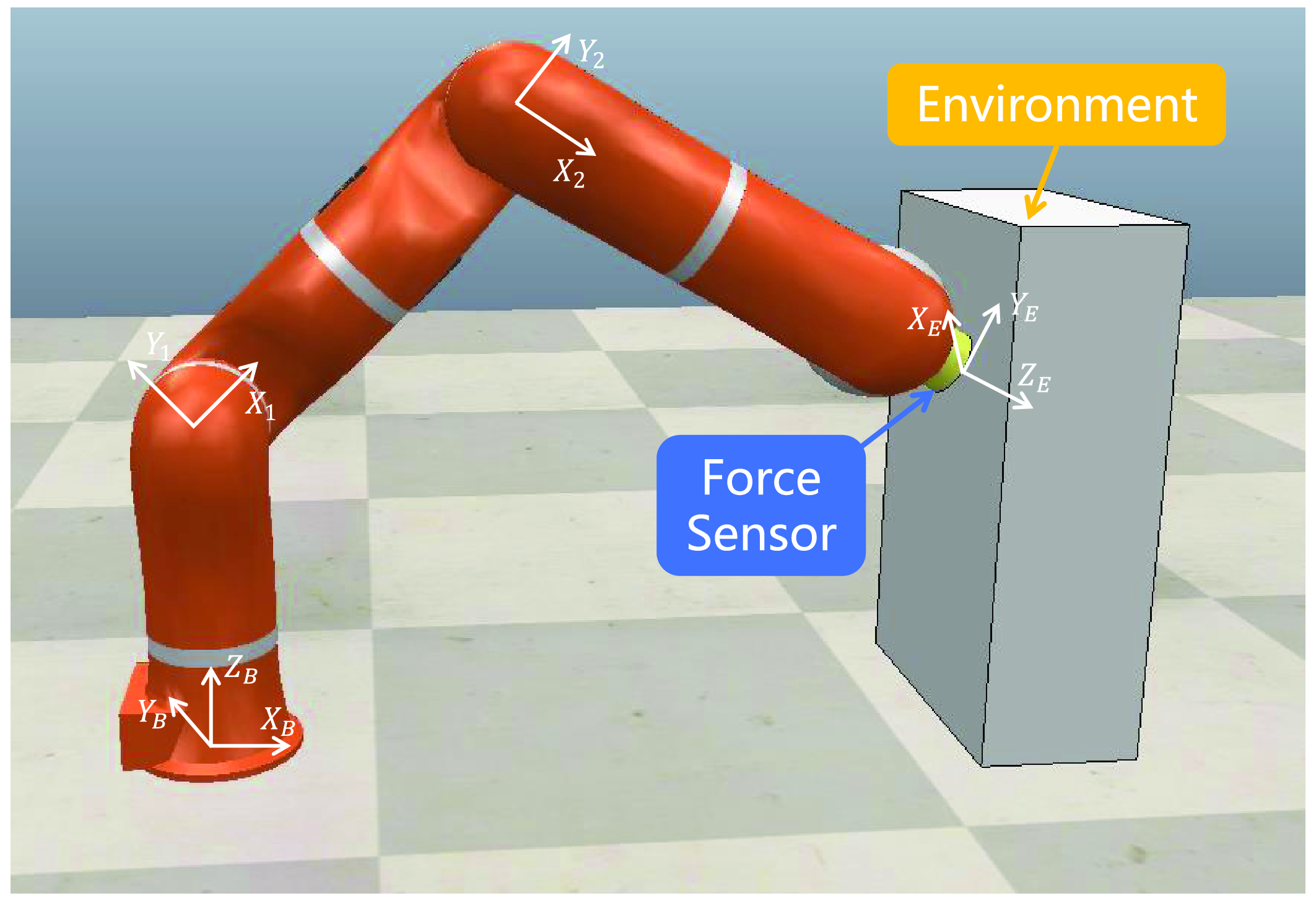
Figure 7. Simulation scenario: the manipulator interacts with the second-order unknown environment in the X-direction.
4. Simulation studies
To verify the interaction and optimal impedance implementation capabilities of the proposed HIAC scheme, simulations are performed on a 2-DOF manipulator in this section. For the simulation setup, the manipulator is considered to interact with the second-order unknown environment, and the external force is applied along the X-direction and can be measured by a force sensor mounted on the end effector, as shown in Fig. 7. In practice, the actual robot dynamics including uncompensated joint friction, model uncertainties, time delays, and noises in the external force measurement are considered in the simulation:
 \begin{equation} {\hat{\boldsymbol{H}}}(\boldsymbol{q})\ddot{\boldsymbol{q}}+{\hat{\boldsymbol{C}}}(\boldsymbol{q},\dot{\boldsymbol{q}})\dot{\boldsymbol{q}}+{\hat{\boldsymbol{G}}}(\boldsymbol{q})=\boldsymbol{\tau}_{\boldsymbol{c}}+\boldsymbol{\tau}_{\boldsymbol{f}}+{\hat{\boldsymbol{J}}}^T(\boldsymbol{q})\hat{\boldsymbol{F}}_{\boldsymbol{e}} \end{equation}
where
 ${\hat{\boldsymbol{H}}}(\boldsymbol{q})$
,
${\hat{\boldsymbol{H}}}(\boldsymbol{q})$
,
 ${\hat{\boldsymbol{C}}}(\boldsymbol{q},\dot{\boldsymbol{q}})$
, and
${\hat{\boldsymbol{C}}}(\boldsymbol{q},\dot{\boldsymbol{q}})$
, and
 ${\hat{\boldsymbol{G}}}(\boldsymbol{q})$
are the estimated inertia matrix, estimated Coriolis and Centrifugal force matrix, and estimated gravitational force vector in joint space, respectively.
${\hat{\boldsymbol{G}}}(\boldsymbol{q})$
are the estimated inertia matrix, estimated Coriolis and Centrifugal force matrix, and estimated gravitational force vector in joint space, respectively.
 ${\hat{\boldsymbol{J}}}$
,
${\hat{\boldsymbol{J}}}$
,
 $\hat{\boldsymbol{F}}_{\boldsymbol{e}}$
, and
$\hat{\boldsymbol{F}}_{\boldsymbol{e}}$
, and
 $\boldsymbol{\tau}_{\boldsymbol{f}}$
are the estimated Jacobian matrix, estimated interaction force, and uncompensated joint friction, respectively. Then, the above kinematic and dynamics parameters are given as:
$\boldsymbol{\tau}_{\boldsymbol{f}}$
are the estimated Jacobian matrix, estimated interaction force, and uncompensated joint friction, respectively. Then, the above kinematic and dynamics parameters are given as:
 \begin{align} {\hat{\boldsymbol{H}}}(\boldsymbol{q})&= \begin{bmatrix}{\hat{m}_2}l_2^2+2{\hat{m}_2}{l_1}{l_2}{c_2}+(\hat{m}_1+\hat{m}_2)l_1^2 & \quad {\hat{m}_2}l_2^2+{\hat{m}_2}{l_1}{l_2}{c_2} \\[5pt]{\hat{m}_2}l_2^2+{\hat{m}_2}{l_1}{l_2}{c_2} &\quad {\hat{m}_2}l_2^2 \end{bmatrix} \notag \\[5pt] {\hat{\boldsymbol{C}}}(\boldsymbol{q},\dot{\boldsymbol{q}}) &= \begin{bmatrix} -{\hat{m}_2}{l_1}{l_2}{s_2}{\dot{q}_2} & \quad -{\hat{m}_2}{l_1}{l_2}{s_2}(\dot{q}_1+\dot{q}_2) \\[5pt]{\hat{m}_2}{l_1}{l_2}{s_2}{\dot{q}_1} & \quad 0 \end{bmatrix}, {\hat{\boldsymbol{G}}}(\boldsymbol{q})= \begin{bmatrix}{\hat{m}_2}{l_2}g{c_{12}}+(\hat{m}_1+\hat{m}_2){l_1}g{c_1} \\[5pt]{\hat{m}_2}{l_2}g{c_{12}} \end{bmatrix} \notag \\[5pt] {\hat{\boldsymbol{J}}}&= \begin{bmatrix} -({l_1}{s_1}+{l_2}{s_{12}})+g_n & \quad -{l_2}{s_{12}}+g_n \\[5pt]{l_1}{c_1}+{l_2}{c_{12}}+g_n & \quad {l_2}{c_{12}}+g_n \end{bmatrix}, \boldsymbol{\tau}_{\boldsymbol{f}}= -\begin{bmatrix} c_v\dot{q}_1+\mathrm{sign}(\dot{q}_1)\tau _c \\[5pt] c_v\dot{q}_2+\mathrm{sign}(\dot{q}_2)\tau _c \end{bmatrix} \notag \\[5pt] \hat{\boldsymbol{F}}_{\boldsymbol{e}}(t)&=\boldsymbol{F}_{\boldsymbol{e}}(t-6{t_s})+[g_n,g_n]^T \end{align}
where the sampling time of the simulations is set as
 $t_s=1$
ms and
$t_s=1$
ms and
 $g_n\sim \mathcal{N}(0, 0.01)$
is the Gaussian noise. Table I presents the parameters of the simulated manipulator. The parameters of the second-order environments are described by:
$g_n\sim \mathcal{N}(0, 0.01)$
is the Gaussian noise. Table I presents the parameters of the simulated manipulator. The parameters of the second-order environments are described by:
 \begin{equation} \boldsymbol{H}_{\boldsymbol{m}}=\begin{bmatrix} 0.1 & \quad 0 \\[4pt] 0 & \quad 0 \end{bmatrix}, \boldsymbol{C}_{\boldsymbol{m}}=\begin{bmatrix} 1 & \quad 0 \\[4pt] 0 & \quad 0 \end{bmatrix}, \boldsymbol{G}_{\boldsymbol{m}}=\begin{bmatrix} k_e & \quad 0 \\[4pt] 0 & \quad 0 \end{bmatrix} \end{equation}
where
 $k_e$
is the environmental stiffness in the X-direction. The soft, medium, and stiff environments corresponding to the environments with low stiffness
$k_e$
is the environmental stiffness in the X-direction. The soft, medium, and stiff environments corresponding to the environments with low stiffness
 $k_e=20$
N/m, medium stiffness
$k_e=20$
N/m, medium stiffness
 $k_e=150$
N/m, and high stiffness
$k_e=150$
N/m, and high stiffness
 $k_e=1000$
N/m, respectively, are considered and assumed to have the same inertia and damping. Note that the environmental parameters are unknown in the simulation.
$k_e=1000$
N/m, respectively, are considered and assumed to have the same inertia and damping. Note that the environmental parameters are unknown in the simulation.
Table I. Parameters of the simulated manipulator.
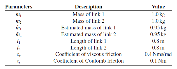
4.1. Interaction capability
In this part, the effectiveness of the proposed impedance adaptation method is verified and the parameters are considered only in the X-direction. The parameters in (21) are set as
 $U=-0.5$
and
$U=-0.5$
and
 $V=0.3$
. The weights in (24) are set as
$V=0.3$
. The weights in (24) are set as
 $Q_1=1$
,
$Q_1=1$
,
 $Q_2=30,000$
, and
$Q_2=30,000$
, and
 $R=1$
to cope with the environments (64) which cover a wide range of stiffness. The initial feedback gain is chosen as
$R=1$
to cope with the environments (64) which cover a wide range of stiffness. The initial feedback gain is chosen as
 $\boldsymbol{K}_{\textbf{0}}=[{-}1,-1500,1500]^T$
, and the initial
$\boldsymbol{K}_{\textbf{0}}=[{-}1,-1500,1500]^T$
, and the initial
 $\boldsymbol{Y}_{\boldsymbol{k}}$
is set as
$\boldsymbol{Y}_{\boldsymbol{k}}$
is set as
 ${\boldsymbol{Y}}_{\textbf{0}}=10\boldsymbol{I}_{\boldsymbol{m}}$
. The exploration noise is designed as
${\boldsymbol{Y}}_{\textbf{0}}=10\boldsymbol{I}_{\boldsymbol{m}}$
. The exploration noise is designed as
 $\nu =-\sum _{\omega =1}^{4}(180/\omega )\sin\! (\omega{t})$
. The preset threshold is set as
$\nu =-\sum _{\omega =1}^{4}(180/\omega )\sin\! (\omega{t})$
. The preset threshold is set as
 $\varepsilon =0.001$
, and the transitional time is set as
$\varepsilon =0.001$
, and the transitional time is set as
 $T_s=2$
s.
$T_s=2$
s.
The simulation results are presented in Figs. 8 and 9. LQR is regarded as the comparison method which can solve ARE using the known matrices
 $\boldsymbol{A}$
and
$\boldsymbol{A}$
and
 $\boldsymbol{B}$
to obtain the optimal target impedance model, while the proposed method is suitable for the case where the environment dynamics are unknown, that is, the matrices
$\boldsymbol{B}$
to obtain the optimal target impedance model, while the proposed method is suitable for the case where the environment dynamics are unknown, that is, the matrices
 $\boldsymbol{A}$
and
$\boldsymbol{A}$
and
 $\boldsymbol{B}$
are unknown. The virtual equilibrium trajectories and actual trajectories of LQR and the proposed method in the soft, medium, and stiff environments are shown in Fig. 8. In any case, an obvious error exists in the actual trajectories between LQR and the proposed method in phase 1 (yellow region) due to the obvious difference between the target impedance model
$\boldsymbol{B}$
are unknown. The virtual equilibrium trajectories and actual trajectories of LQR and the proposed method in the soft, medium, and stiff environments are shown in Fig. 8. In any case, an obvious error exists in the actual trajectories between LQR and the proposed method in phase 1 (yellow region) due to the obvious difference between the target impedance model
 $F_e=\ddot{x}+\dot{x}+1500(x-x_0)+\nu$
equivalent to the initial system input and the optimal target impedance model obtained by LQR. In addition, the exploration noise results in trajectory jitters of the proposed method, which is inevitable because rich state and input information is required to ensure that the system meets the PE condition so that the rank condition (14) is satisfied. In phase 2 (blue region), the transitional system input works so that the trajectory error rises slightly for a short time and then decreases smoothly. In phase 3 (green region), the actual trajectory of the proposed method converges to a small neighborhood of the actual trajectory of LQR.
$F_e=\ddot{x}+\dot{x}+1500(x-x_0)+\nu$
equivalent to the initial system input and the optimal target impedance model obtained by LQR. In addition, the exploration noise results in trajectory jitters of the proposed method, which is inevitable because rich state and input information is required to ensure that the system meets the PE condition so that the rank condition (14) is satisfied. In phase 2 (blue region), the transitional system input works so that the trajectory error rises slightly for a short time and then decreases smoothly. In phase 3 (green region), the actual trajectory of the proposed method converges to a small neighborhood of the actual trajectory of LQR.
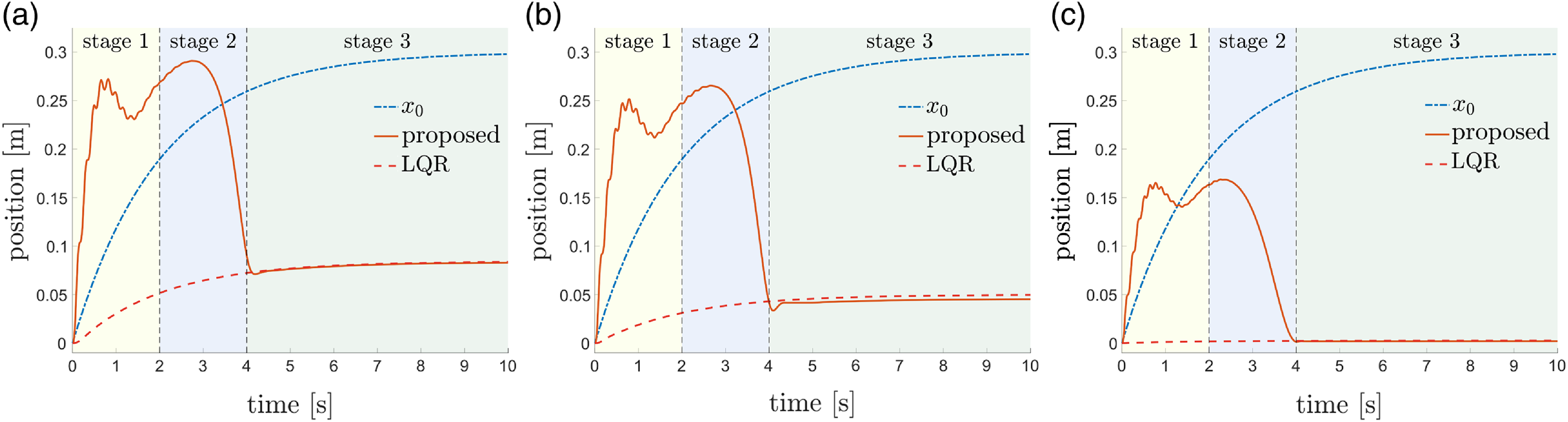
Figure 8. Virtual equilibrium and actual trajectories in the (a) soft, (b) medium, and (c) stiff environments. For the proposed method, in stage 1 (yellow region), the system input is set as
 $\boldsymbol{u}=-\boldsymbol{K}_{\textbf{0}}\boldsymbol{\xi }+\boldsymbol{\nu }$
and the system information is collected until the rank condition (14) is satisfied. In stage 2 (blue region), the optimal feedback gain
$\boldsymbol{u}=-\boldsymbol{K}_{\textbf{0}}\boldsymbol{\xi }+\boldsymbol{\nu }$
and the system information is collected until the rank condition (14) is satisfied. In stage 2 (blue region), the optimal feedback gain
 $\boldsymbol{K}_{\boldsymbol{k}}$
is solved, and the system input is set as
$\boldsymbol{K}_{\boldsymbol{k}}$
is solved, and the system input is set as
 $\boldsymbol{u}=-\boldsymbol{K}^{\prime}_{\boldsymbol{k}}\boldsymbol{\xi }+\boldsymbol{\nu}^{\prime}$
to keep the system input continuous until
$\boldsymbol{u}=-\boldsymbol{K}^{\prime}_{\boldsymbol{k}}\boldsymbol{\xi }+\boldsymbol{\nu}^{\prime}$
to keep the system input continuous until
 $t\gt t_l+T_s$
. In stage 3 (green region), the system input becomes
$t\gt t_l+T_s$
. In stage 3 (green region), the system input becomes
 $\boldsymbol{u}=-\boldsymbol{K}_{\boldsymbol{k}}\boldsymbol{\xi }$
.
$\boldsymbol{u}=-\boldsymbol{K}_{\boldsymbol{k}}\boldsymbol{\xi }$
.

Figure 9. Impedance parameters in the (a) soft, (b) medium, and (c) stiff environments.
 $\boldsymbol{C}_{\boldsymbol{d}}$
,
$\boldsymbol{C}_{\boldsymbol{d}}$
,
 $\boldsymbol{K}_{\boldsymbol{d}}$
, and
$\boldsymbol{K}_{\boldsymbol{d}}$
, and
 $\boldsymbol{K}^{\prime}_{\boldsymbol{d}}$
are adapted by the proposed method.
$\boldsymbol{K}^{\prime}_{\boldsymbol{d}}$
are adapted by the proposed method.
 $\boldsymbol{C}^*_{\boldsymbol{d}}$
,
$\boldsymbol{C}^*_{\boldsymbol{d}}$
,
 $\boldsymbol{K}^*_{\boldsymbol{d}}$
, and
$\boldsymbol{K}^*_{\boldsymbol{d}}$
, and
 $\boldsymbol{K}^{\prime *}_{\boldsymbol{d}}$
are solved by LQR.
$\boldsymbol{K}^{\prime *}_{\boldsymbol{d}}$
are solved by LQR.
The impedance parameters of LQR and the proposed method in the soft, medium, and stiff environments are shown in Fig. 9. The impedance parameters adapted by the proposed method change smoothly during stage 2 and converges to a small neighborhood of the impedance parameters of LQR in stage 3. Table II presents the target impedance models obtained by LQR and the proposed method in the soft, medium, and stiff environments. It can be seen that the models obtained by the proposed method are second-order and are quite close to the corresponding optimal models obtained by LQR in the second-order environments, which proves the ability of the proposed method to obtain the target impedance model representing the optimal interaction behavior without the accurate environment dynamics. Moreover, it is noteworthy that as the environmental stiffness increases, the desired stiffness and damping of the target impedance model obtained by the proposed method decrease. In other words, as the environment becomes stiffer, the desired interaction behavior obtained by the proposed method becomes softer, which shows good adaptability of the proposed method to different environments.
Table II. Simulated target impedance models.
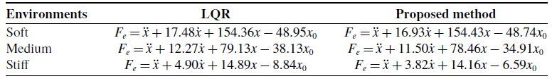
4.2. Impedance implementation capability
In this part, a fixed target impedance model is implemented in the environments (64) to illustrate the effectiveness of the proposed hybrid system framework. Specifically, the switching control law (35) is implemented using (28) and (32), and the desired trajectory
 $\boldsymbol{x}_{\boldsymbol{d}}$
is updated using (37) and (31) during impedance and admittance control phases, respectively. Note that the ideal trajectory
$\boldsymbol{x}_{\boldsymbol{d}}$
is updated using (37) and (31) during impedance and admittance control phases, respectively. Note that the ideal trajectory
 $\boldsymbol{x}_{\boldsymbol{ref}}$
is not used in the control process. The parameters of the fixed target impedance model to be implemented are chosen as
$\boldsymbol{x}_{\boldsymbol{ref}}$
is not used in the control process. The parameters of the fixed target impedance model to be implemented are chosen as
 $\boldsymbol{H}_{\boldsymbol{d}}=1.0{\boldsymbol{I}}_{\textbf{2}}$
,
$\boldsymbol{H}_{\boldsymbol{d}}=1.0{\boldsymbol{I}}_{\textbf{2}}$
,
 $\boldsymbol{C}_{\boldsymbol{d}}=4{\boldsymbol{I}}_{\textbf{2}}$
,
$\boldsymbol{C}_{\boldsymbol{d}}=4{\boldsymbol{I}}_{\textbf{2}}$
,
 $\boldsymbol{K}_{\boldsymbol{d}}=10{\boldsymbol{I}}_{\textbf{2}}$
, and
$\boldsymbol{K}_{\boldsymbol{d}}=10{\boldsymbol{I}}_{\textbf{2}}$
, and
 $\boldsymbol{K}^{\prime}_{\boldsymbol{d}}=5{\boldsymbol{I}}_{\textbf{2}}$
. The switching period is designed as
$\boldsymbol{K}^{\prime}_{\boldsymbol{d}}=5{\boldsymbol{I}}_{\textbf{2}}$
. The switching period is designed as
 $\delta =0.02$
s, and the control gains of the inner loop controller of admittance control are designed with high gain as
$\delta =0.02$
s, and the control gains of the inner loop controller of admittance control are designed with high gain as
 $\boldsymbol{L}_{\boldsymbol{p}}=10^6{\boldsymbol{I}}_{\textbf{2}}$
and
$\boldsymbol{L}_{\boldsymbol{p}}=10^6{\boldsymbol{I}}_{\textbf{2}}$
and
 $\boldsymbol{L}_{\boldsymbol{v}}=500{\boldsymbol{I}}_{\textbf{2}}$
to be robust to the system uncertainties and make
$\boldsymbol{L}_{\boldsymbol{v}}=500{\boldsymbol{I}}_{\textbf{2}}$
to be robust to the system uncertainties and make
 $\boldsymbol{A}_{\boldsymbol{eq}}$
Hurwitz. The virtual equilibrium trajectory in the X-direction is designed as
$\boldsymbol{A}_{\boldsymbol{eq}}$
Hurwitz. The virtual equilibrium trajectory in the X-direction is designed as
 $x_0=1+\sin\! (8t)$
m.
$x_0=1+\sin\! (8t)$
m.
The ideal trajectories
 $\boldsymbol{x}_{\boldsymbol{ref}}$
for the fixed target impedance model in different environments are calculated by (38) and shown in Fig. 10(a). The trajectory errors of different controllers for the fixed target impedance model in the soft, medium, and stiff environments are shown in Fig. 10(b)–(d), respectively, where impedance, admittance, and the intermediate controllers with different duty cycle parameters are introduced. In the soft environment, impedance control results in relatively large tracking error and steady-state error due to the uncompensated friction, while admittance control has better performance, which is shown as high position accuracy. As the environmental stiffness increases, the performance of impedance control improves, shown as the decrease in steady-state error, while the performance of admittance control deteriorates, shown as the increase in oscillations, due to the time delay of the external force measurement and the high gains of the inner loop controller. Finally, for the stiff environment, admittance control leads to large oscillations, while impedance control imparts good robustness to the system, which is shown as small oscillations and negligible steady-state error.
$\boldsymbol{x}_{\boldsymbol{ref}}$
for the fixed target impedance model in different environments are calculated by (38) and shown in Fig. 10(a). The trajectory errors of different controllers for the fixed target impedance model in the soft, medium, and stiff environments are shown in Fig. 10(b)–(d), respectively, where impedance, admittance, and the intermediate controllers with different duty cycle parameters are introduced. In the soft environment, impedance control results in relatively large tracking error and steady-state error due to the uncompensated friction, while admittance control has better performance, which is shown as high position accuracy. As the environmental stiffness increases, the performance of impedance control improves, shown as the decrease in steady-state error, while the performance of admittance control deteriorates, shown as the increase in oscillations, due to the time delay of the external force measurement and the high gains of the inner loop controller. Finally, for the stiff environment, admittance control leads to large oscillations, while impedance control imparts good robustness to the system, which is shown as small oscillations and negligible steady-state error.

Figure 10. (a) Virtual equilibrium and ideal trajectories. Trajectory errors of different controllers for the fixed target impedance model in the (b) soft, (c) medium, and (d) stiff environments.
Moreover, it can be seen from Fig. 10 that the response of the intermediate controller corresponding to a smaller duty cycle is closer to the response of impedance control, and as the duty cycle increases, it tends to the response of admittance control. Therefore, the proposed framework can generate interpolation between the responses of impedance control and admittance control by properly selecting the duty cycle, showing its applicability to the second-order environments and its potential to provide good control performance independent of the environmental stiffness, which is illustrated in the following section.
4.3. Optimal implementation capability
In this part, the proposed hybrid system framework’s capability to provide the optimal implementation performance for the target impedance models using the mapping of the optimal duty cycle is evaluated. The initial time and end time of control are set as
 $t_u=0$
s and
$t_u=0$
s and
 $t_f=2$
s, respectively. The target impedance models to be implemented are obtained by the proposed impedance adaptation method and shown in Table II. The remaining parameters are the same as above. Considering the desired stiffness
$t_f=2$
s, respectively. The target impedance models to be implemented are obtained by the proposed impedance adaptation method and shown in Table II. The remaining parameters are the same as above. Considering the desired stiffness
 $k_d^*$
in range
$k_d^*$
in range
 $[10,170]$
, the mapping is built offline and shown in Fig. 11(a), where we can see that the optimal duty cycle becomes larger as the desired behavior becomes stiffer, and the optimal duty cycle has a minimum interval of
$[10,170]$
, the mapping is built offline and shown in Fig. 11(a), where we can see that the optimal duty cycle becomes larger as the desired behavior becomes stiffer, and the optimal duty cycle has a minimum interval of
 $t_s/\delta =0.05$
between
$t_s/\delta =0.05$
between
 $[0,1]$
. The optimal duty cycles corresponding to the desired stiffness in the soft, medium, and stiff environments can be obtained as
$[0,1]$
. The optimal duty cycles corresponding to the desired stiffness in the soft, medium, and stiff environments can be obtained as
 $\alpha ^*=0.85$
,
$\alpha ^*=0.85$
,
 $\alpha ^*=0.55$
, and
$\alpha ^*=0.55$
, and
 $\alpha ^*=0.3$
from the mapping, respectively. It should be noted that the estimated environmental stiffness is implicitly used as an intermediate variable during this process as shown in (61), and the target impedance models remain constant after impedance adaptation.
$\alpha ^*=0.3$
from the mapping, respectively. It should be noted that the estimated environmental stiffness is implicitly used as an intermediate variable during this process as shown in (61), and the target impedance models remain constant after impedance adaptation.

Figure 11. (a) Mapping of the optimal duty cycle in the simulation. (b) Virtual equilibrium and ideal trajectories. The trajectory errors of different controllers for the corresponding target impedance models in the (c) soft, (d) medium, and (e) stiff environments.
Figure 11(b) shows the virtual equilibrium and ideal trajectories for the corresponding target impedance models in different environments. The trajectory errors of different controllers for the corresponding target impedance model in the soft, medium, and stiff environments are shown in Fig. 11(c)–(e), where impedance, admittance, and the intermediate controllers corresponding to different duty cycles are introduced. In Fig. 11(c)–(e), impedance control and admittance control show similar characteristics to those in the previous section for the same environment. In the soft environment, the response of the optimal intermediate controller is close to the response of admittance control, and a higher position accuracy than that of admittance control is obtained. In the medium environment, the response of the optimal intermediate controller tends to be the average of the responses of impedance and admittance controls, resulting in better tracking performance than both controllers. In the stiff environment, the response of the optimal intermediate controller tends to the response of impedance control, showing its good robustness. In addition, compared with the other two intermediate controllers, the optimal intermediate controller shows better tracking performance in different environments.
5. Experimental studies
In this section, the performance of the robot–environment interaction using the proposed HIAC scheme is demonstrated by experiments conducted on a 7-DOF Franka EMIKA panda robot, as shown in Fig. 12. For the experimental setup, the robot is connected to a workstation PC via Ethernet, and the Franka Control Interface (FCI) is used to achieve the real-time control loop running at 1 kHz. Meanwhile, the current status of the robot including the interaction force between the robot and the objects are obtained from FCI at 1 kHz. In the experiment, the robot will contact with the soft and stiff sponge objects along the z-axis using the proposed HIAC scheme and the comparison method. On the z-axis, the soft object’s inertia, damping, and stiffness parameters are 0.1 kg, 2 Ns/m, and 500 N/m, respectively. The stiff object’s inertia, damping, and stiffness parameters are 0.1 kg, 5 Ns/m, and 1500 N/m, respectively. First, the end-effector position of the robot is moved to
 $[0.36, 0, 0.08]$
m, then it will contact with the objects by specifying the virtual equilibrium trajectory as:
$[0.36, 0, 0.08]$
m, then it will contact with the objects by specifying the virtual equilibrium trajectory as:
 \begin{equation} \boldsymbol{x}_{\textbf{0}}=\begin{bmatrix} 0.36, & 0, & 0.08-0.05(1-\exp (-t)) \end{bmatrix}^T \end{equation}
To proceed, an experimental comparison between the proposed impedance adaptation method and the commonly used LQR method is conducted to obtain the optimal impedance parameters. In this part, the weights in (24) are set as
 $Q_1=1$
,
$Q_1=1$
,
 $Q_2=1000$
, and
$Q_2=1000$
, and
 $R=0.001$
. The initial feedback gain is chosen as
$R=0.001$
. The initial feedback gain is chosen as
 $\boldsymbol{K}_{\textbf{0}}=[{-}100,-2500,2500]^T$
, and the initial
$\boldsymbol{K}_{\textbf{0}}=[{-}100,-2500,2500]^T$
, and the initial
 $\boldsymbol{Y}_{\boldsymbol{k}}$
is set as
$\boldsymbol{Y}_{\boldsymbol{k}}$
is set as
 ${\boldsymbol{Y}}_{\textbf{0}}=\boldsymbol{I}_{\boldsymbol{m}}$
. The parameters in (21) are set as
${\boldsymbol{Y}}_{\textbf{0}}=\boldsymbol{I}_{\boldsymbol{m}}$
. The parameters in (21) are set as
 $U=-0.3$
and
$U=-0.3$
and
 $V=0.6$
, and the exploration noise is designed as
$V=0.6$
, and the exploration noise is designed as
 $\nu =-\sum _{\omega =1}^{8}\!(10/\omega )\sin\! (\omega{t})$
. For the proposed method, the impedance iteration will stop when
$\nu =-\sum _{\omega =1}^{8}\!(10/\omega )\sin\! (\omega{t})$
. For the proposed method, the impedance iteration will stop when
 $\Vert{\boldsymbol{Y}_{\boldsymbol{k}}}-\boldsymbol{Y}_{\boldsymbol{k}-\textbf{1}}\Vert \leq 0.001$
and the transition begins with the transitional time
$\Vert{\boldsymbol{Y}_{\boldsymbol{k}}}-\boldsymbol{Y}_{\boldsymbol{k}-\textbf{1}}\Vert \leq 0.001$
and the transition begins with the transitional time
 $T_s=2$
s. However, for the LQR method, an accurate environment dynamics model is required to obtain the optimal impedance parameters through the Riccati equation [Reference Lewis, Vrabie and Syrmos21]. The experimental results are presented in Figs. 13–17. It can be seen that after impedance adaptation, the interaction behavior of the proposed method, including actual trajectory, interaction force, and impedance parameters, are close to those of the LQR method, which is consistent with the simulation results.
$T_s=2$
s. However, for the LQR method, an accurate environment dynamics model is required to obtain the optimal impedance parameters through the Riccati equation [Reference Lewis, Vrabie and Syrmos21]. The experimental results are presented in Figs. 13–17. It can be seen that after impedance adaptation, the interaction behavior of the proposed method, including actual trajectory, interaction force, and impedance parameters, are close to those of the LQR method, which is consistent with the simulation results.
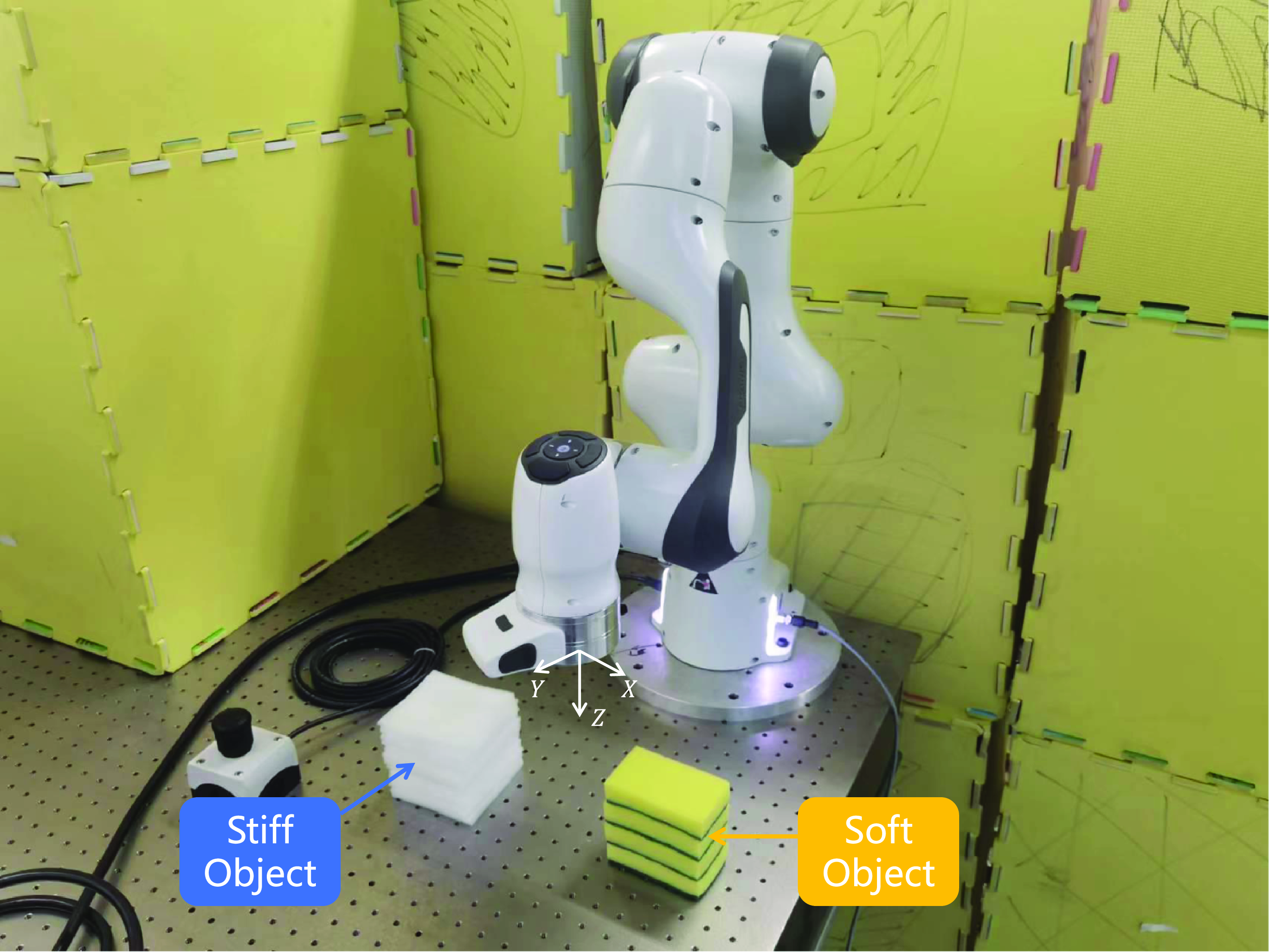
Figure 12. Experimental scenario: Franka EMIKA panda robot interacts with the soft and stiff objects.
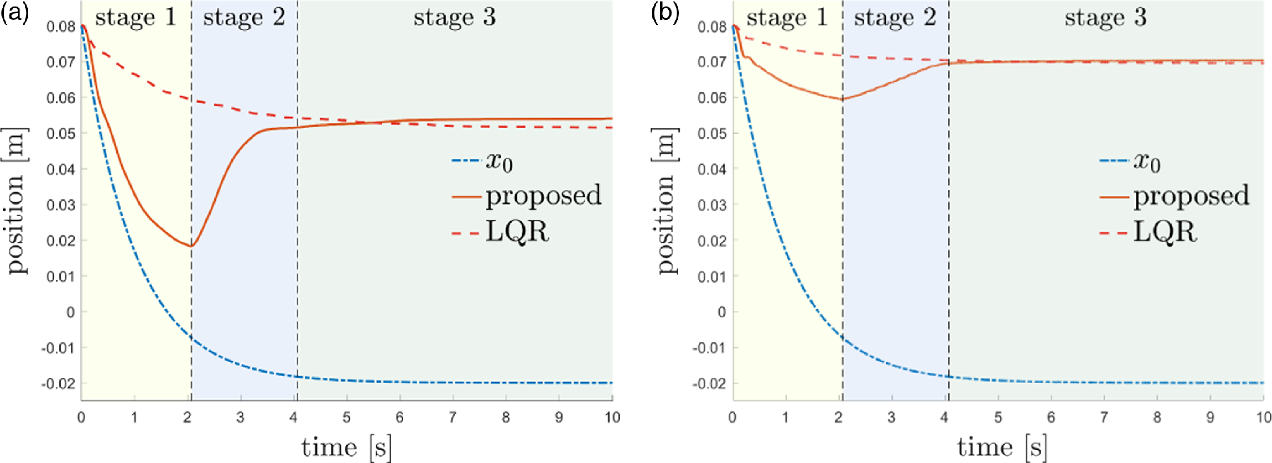
Figure 13. Virtual equilibrium and actual experimental trajectories for the (a) soft and (b) stiff objects. The introduction of each stage is the same as Fig. 8.
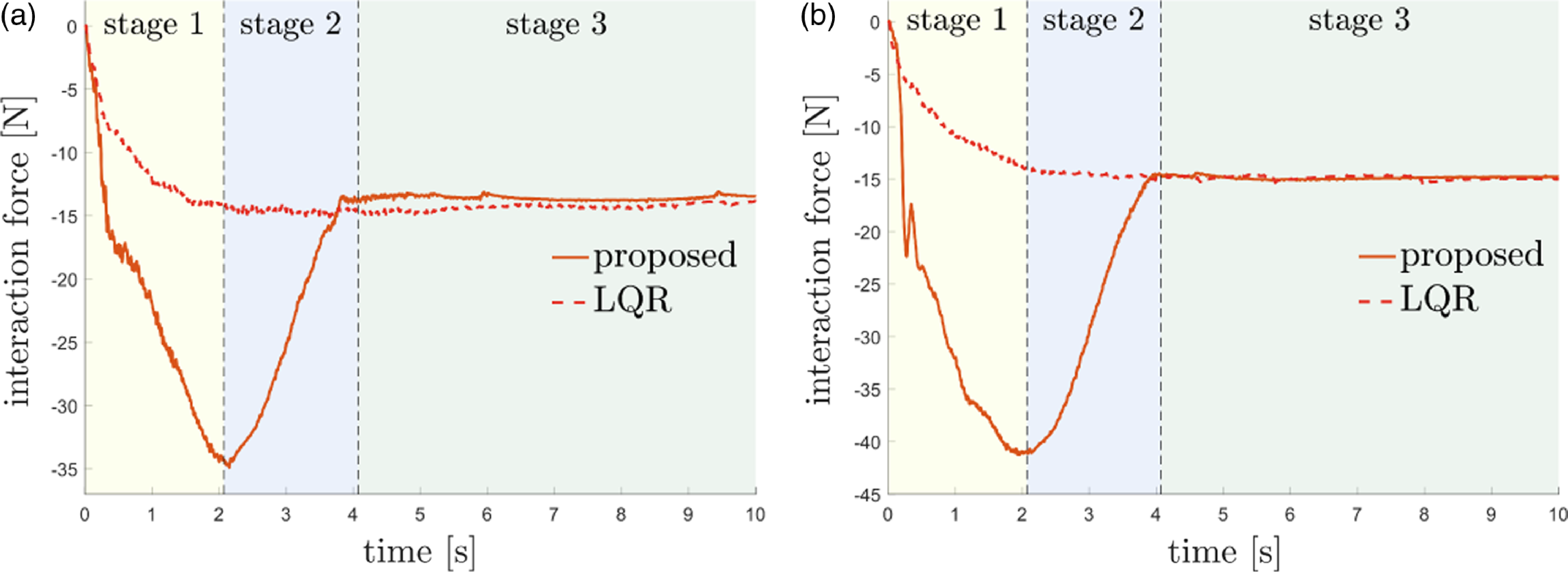
Figure 14. Experimental interaction forces for the (a) soft and (b) stiff objects.

Figure 15. Experimental impedance parameters for the (a) soft and (b) stiff objects.

Figure 16. Errors of experimental impedance parameters for the (a) soft and (b) stiff objects.
To further show the convergence performance of the impedance parameters obtained by the proposed method to the optimal values obtained by LQR more clearly, the errors of impedance parameters defined as
 $\Vert \boldsymbol{K}_{\boldsymbol{k}}-{\boldsymbol{K}}^*\Vert$
are illustrated in Fig. 16, where the error decreases to around 5.92 after seven iterations for the soft object and decreases to around 6.45 after eight iterations for the stiff object. Table III presents the target impedance models obtained by LQR and the proposed method for the soft and stiff objects. It can be seen that the experimental error of damping parameters of the proposed method increases compared to simulation, which is mainly due to the influence of external noises on the velocity and force data collected in the experiment. In addition, Fig. 17 shows the control torques of seven robot joints during impedance adaptation for the soft and stiff objects. The maximum and average control torques for the interaction with the stiff object are larger than the soft object, and the second, fourth, and sixth joints bear the main output in the interaction.
$\Vert \boldsymbol{K}_{\boldsymbol{k}}-{\boldsymbol{K}}^*\Vert$
are illustrated in Fig. 16, where the error decreases to around 5.92 after seven iterations for the soft object and decreases to around 6.45 after eight iterations for the stiff object. Table III presents the target impedance models obtained by LQR and the proposed method for the soft and stiff objects. It can be seen that the experimental error of damping parameters of the proposed method increases compared to simulation, which is mainly due to the influence of external noises on the velocity and force data collected in the experiment. In addition, Fig. 17 shows the control torques of seven robot joints during impedance adaptation for the soft and stiff objects. The maximum and average control torques for the interaction with the stiff object are larger than the soft object, and the second, fourth, and sixth joints bear the main output in the interaction.
Table III. Experimental target impedance models.
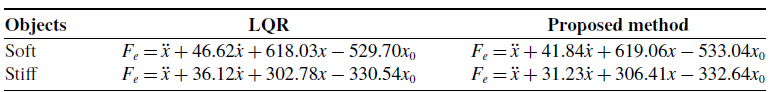
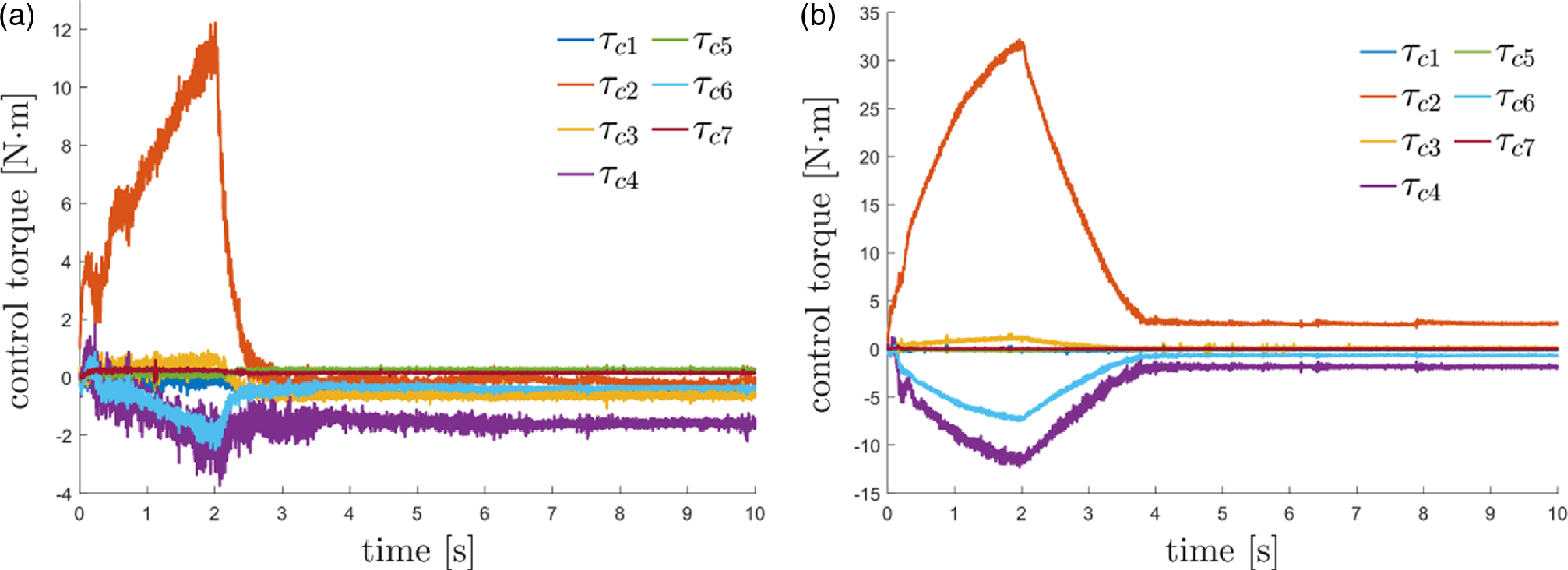
Figure 17. Control torques of seven robot joints during impedance adaptation for the (a) soft and (b) stiff objects.
Then, the proposed hybrid system framework is utilized to obtain the optimal implementation performance for the target impedance models using the mapping of the optimal duty cycle and compared with the hybrid controller in ref. [Reference Cavenago, Voli and Massari32]. For both the proposed and the comparison method, the initial time and end time of control are set as
 $t_u=0$
s and
$t_u=0$
s and
 $t_f=10$
s, respectively. The switching period is designed as
$t_f=10$
s, respectively. The switching period is designed as
 $\delta =0.02$
s, and the inner loop control gains of admittance control are designed as
$\delta =0.02$
s, and the inner loop control gains of admittance control are designed as
 $L_p=2000$
and
$L_p=2000$
and
 $L_v=1.4\sqrt{L_p}$
on the z-axis. The virtual equilibrium trajectory is the same as (65). Considering that the robot–environment interaction dynamics has been decoupled by the designed controller in each direction, the mapping of the optimal duty cycle on the z-axis for the proposed method in the experiment is generated through simulation using the above parameters, as shown in Fig. 18(a). According to the target impedance models in Table III, the optimal duty cycles of the proposed controller corresponding to the desired stiffness for the soft and stiff objects are obtained as
$L_v=1.4\sqrt{L_p}$
on the z-axis. The virtual equilibrium trajectory is the same as (65). Considering that the robot–environment interaction dynamics has been decoupled by the designed controller in each direction, the mapping of the optimal duty cycle on the z-axis for the proposed method in the experiment is generated through simulation using the above parameters, as shown in Fig. 18(a). According to the target impedance models in Table III, the optimal duty cycles of the proposed controller corresponding to the desired stiffness for the soft and stiff objects are obtained as
 $\alpha ^*=0.7$
and
$\alpha ^*=0.7$
and
 $\alpha ^*=0.5$
from the mapping, respectively. The optimal duty cycles of the hybrid controller in ref. [Reference Cavenago, Voli and Massari32] are assumed to be the same as those of the proposed controller.
$\alpha ^*=0.5$
from the mapping, respectively. The optimal duty cycles of the hybrid controller in ref. [Reference Cavenago, Voli and Massari32] are assumed to be the same as those of the proposed controller.

Figure 18. (a) Mapping of the optimal duty cycle in the experiment. (b) Virtual equilibrium and ideal experimental trajectories. The trajectory errors of different controllers for the corresponding target impedance models for the (c) soft and (d) stiff objects.
To proceed, Fig. 18(b) shows the virtual equilibrium and ideal trajectories for the corresponding target impedance models. The trajectory errors of different controllers for the soft and stiff objects are illustrated in Fig. 18(c) and (d), where impedance, admittance, and the intermediate controllers corresponding to different duty cycles and the comparison controller in ref. [Reference Cavenago, Voli and Massari32] are introduced for the soft object, while admittance controller is not used for the stiff object because it will cause system instability. From Fig. 18(c) and (d), it can be seen that at the beginning, admittance controller for the soft object and the intermediate controller corresponding to
 $\alpha =0.85$
for the stiff object cause relatively large oscillations due to their stiff characteristic and the uncertainties of the measured interaction force, while the optimal intermediate controllers have smoother performances and smaller transient tracking errors. Impedance controller results in large transient and steady-state tracking errors in the two cases due to its soft characteristic and unmodeled system dynamics, while the optimal intermediate controller has smaller steady-state errors. In addition, it can be observed that the comparison controller in ref. [Reference Cavenago, Voli and Massari32] initially results in a larger transient tracking error than the proposed controller because it only takes into account the spring environment and lacks feedforward velocity and acceleration terms in the admittance inner loop controller. From the above results, the proposed optimal intermediate controller chosen through the mapping exhibits better trajectory tracking performance than impedance, admittance, and the intermediate controllers corresponding to other duty cycles and the comparison controller in ref. [Reference Cavenago, Voli and Massari32] for the soft and stiff objects. Besides, Figs. 19 and 20 illustrate the control torques of seven robot joints using different controllers for the corresponding target impedance models for the soft and stiff objects, respectively. It can be seen that the switching mechanism of the intermediate controller causes control torque vibration, which is difficult to completely avoid in practice, but can be limited to an acceptable range in the experiment by selecting appropriate parameters. Note that the control torque vibration of the comparison controller in ref. [Reference Cavenago, Voli and Massari32] is smaller than that of the proposed controller. One possible reason is that the admittance inner loop controller in ref. [Reference Cavenago, Voli and Massari32] is designed as a PD regulator, so the desired trajectory can be directly obtained during controller switching instead of its second derivative, thus avoiding integration error.
$\alpha =0.85$
for the stiff object cause relatively large oscillations due to their stiff characteristic and the uncertainties of the measured interaction force, while the optimal intermediate controllers have smoother performances and smaller transient tracking errors. Impedance controller results in large transient and steady-state tracking errors in the two cases due to its soft characteristic and unmodeled system dynamics, while the optimal intermediate controller has smaller steady-state errors. In addition, it can be observed that the comparison controller in ref. [Reference Cavenago, Voli and Massari32] initially results in a larger transient tracking error than the proposed controller because it only takes into account the spring environment and lacks feedforward velocity and acceleration terms in the admittance inner loop controller. From the above results, the proposed optimal intermediate controller chosen through the mapping exhibits better trajectory tracking performance than impedance, admittance, and the intermediate controllers corresponding to other duty cycles and the comparison controller in ref. [Reference Cavenago, Voli and Massari32] for the soft and stiff objects. Besides, Figs. 19 and 20 illustrate the control torques of seven robot joints using different controllers for the corresponding target impedance models for the soft and stiff objects, respectively. It can be seen that the switching mechanism of the intermediate controller causes control torque vibration, which is difficult to completely avoid in practice, but can be limited to an acceptable range in the experiment by selecting appropriate parameters. Note that the control torque vibration of the comparison controller in ref. [Reference Cavenago, Voli and Massari32] is smaller than that of the proposed controller. One possible reason is that the admittance inner loop controller in ref. [Reference Cavenago, Voli and Massari32] is designed as a PD regulator, so the desired trajectory can be directly obtained during controller switching instead of its second derivative, thus avoiding integration error.

Figure 19. Control torques of seven robot joints using different controllers for the corresponding target impedance models for the soft object. (a) Impedance controller, (b) intermediate controller corresponding to
 $\alpha =0.3$
, (c) optimal intermediate controller corresponding to
$\alpha =0.3$
, (c) optimal intermediate controller corresponding to
 $\alpha ^*=0.7$
, (d) admittance controller, and (e) comparison controller.
$\alpha ^*=0.7$
, (d) admittance controller, and (e) comparison controller.
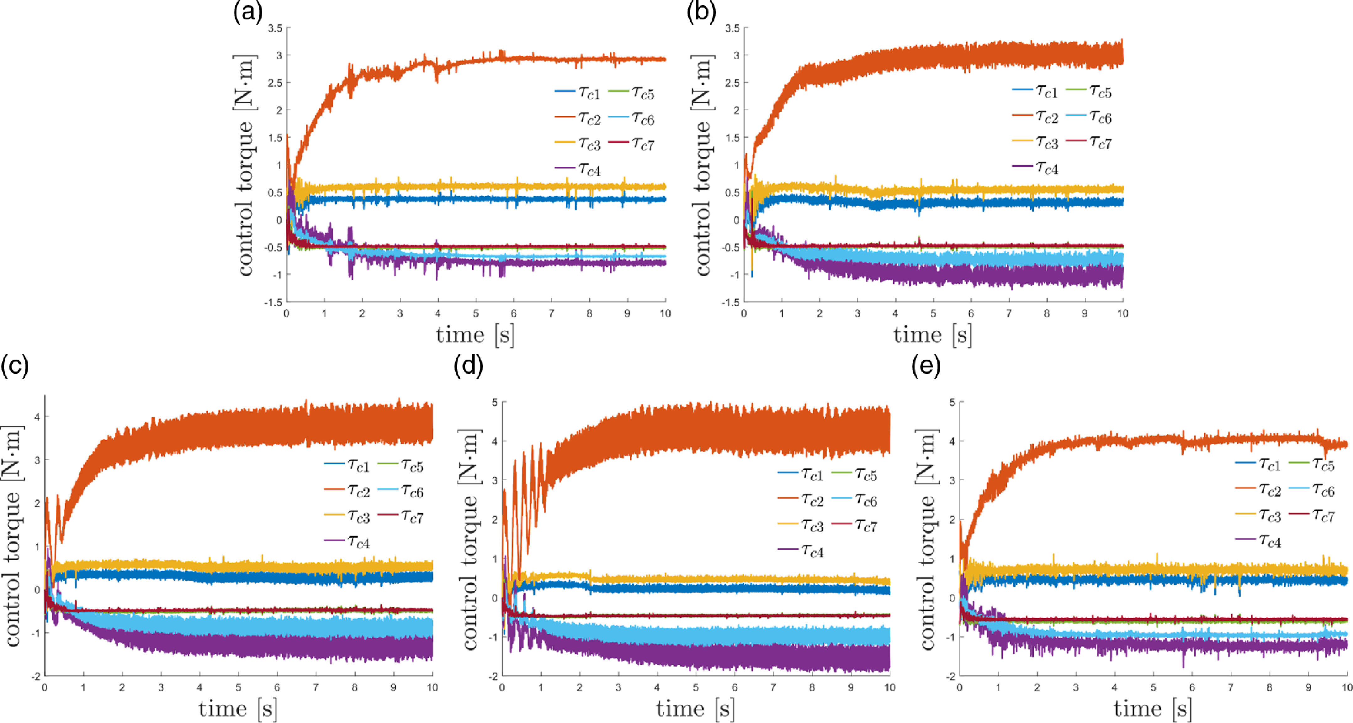
Figure 20. Control torques of seven robot joints using different controllers for the corresponding target impedance models for the stiff object. (a) Impedance controller, (b) intermediate controller corresponding to
 $\alpha =0.2$
, (c) optimal intermediate controller corresponding to
$\alpha =0.2$
, (c) optimal intermediate controller corresponding to
 $\alpha ^*=0.5$
, (d) intermediate controller corresponding to
$\alpha ^*=0.5$
, (d) intermediate controller corresponding to
 $\alpha =0.85$
, (e) and comparison controller.
$\alpha =0.85$
, (e) and comparison controller.
In summary, the proposed impedance adaptation method can obtain the optimal interaction behavior for the robot interacting with different second-order environments using the same control parameters without the accurate environment model; thus, it can be applied in more fields than LQR. The corresponding optimal intermediate controller is selected using the mapping of the optimal duty cycle, which enables the proposed hybrid system framework to combine the advantages of the good robustness of impedance control during stiff contact and the high position accuracy of admittance control during soft contact, thereby achieving better performance than impedance control or admittance control. For the cost function (60), the optimal implementation performance of the obtained target impedance models in different second-order environments is achieved. Therefore, the proposed HIAC scheme can solve the problem of obtaining and implementing optimal interaction behavior in complex unknown environments effectively.
6. Conclusion
In this article, a HIAC scheme is developed for robot manipulators to interact with the second-order unknown environment. An impedance adaptation method with virtual inertia is proposed to make the manipulators have the optimal interaction behavior described by the second-order target impedance model without the need for accurate environment dynamics and acceleration feedback. A hybrid system framework suitable for the second-order environment is proposed to generate a series of intermediate controllers to interpolate between the responses of impedance control and admittance control by adjusting the duty cycle of the switching controller. A mapping of the optimal duty cycle is built to select the optimal intermediate controller to provide the optimal implementation performance for the obtained target impedance model. Simulation and experimental studies on the Franka EMIKA panda robot have verified the effectiveness of the proposed HIAC scheme, and the proposed hybrid system framework shows higher trajectory tracking accuracy than the comparison hybrid controller in the experiment. In practice, robots may need to interact with fast time-varying environments in complex tasks, and free-space/contact phase switching is inevitable during this process. In future work, we will consider improving our scheme to adapt to interactions with fast time-varying environments and integrating the free-space/contact phase switching controller [Reference Roveda, Riva, Bucca and Piga13] into our framework to deal with the impact and force overshoots. Moreover, we will be committed to combining our hybrid controllers and the advanced adaptive impedance controllers [Reference Izadbakhsh and Khorashadizadeh8, Reference Izadbakhsh, Deylami and Khorashadizadeh9] to eliminate the impact of system uncertainties and further improve control performance.
Author contributions
Dexi Ye conceived and designed the study, collected the data, and wrote the manuscript. Yiming Jiang and Hui Zhang analyzed and interpreted the data and wrote the manuscript. Chenguang Yang conceived and designed the study, wrote and revised the manuscript, and supervised the study. All authors have read and approved the final manuscript.
Financial support
This work was supported in part by National Nature Science Foundation of China (NSFC) under Grant U20A20200, Grant 92148204 and Grant 62003136, in part by Guangdong Basic and Applied Basic Research Foundation under Grant 2020B1515120054, in part by Industrial Key Technologies R & D Program of Foshan under Grant 2020001006308 and Grant 2020001006496, and in part by the Open Research Fund from Guangdong Laboratory of Artificial Intelligence and Digital Economy (SZ) (GML-KF-22-14).
Competing interests
The authors declare that the research was conducted in the absence of any commercial or financial relationships that could be construed as a potential conflict of interest.
Ethical approval
None.


