


1. Introduction
Vortex meandering is the prototype of the slow response dynamics of an isolated line vortex evolving in an environment of weakly-structured disturbances. As such, it is documented to affect a large variety of vortex-dominated flows from engineering to geophysics. Prominent examples include experiments and simulations of trailing vortices (Devenport et al. Reference Devenport, Rife, Liapis and Follin1996; Jammy, Hills & Birch Reference Jammy, Hills and Birch2014; Bailey et al. Reference Bailey, Pentelow, Ghimire, Estejab, Green and Tavoularis2018), inlet vortices (Wang & Gursul Reference Wang and Gursul2012) and tornadoes (Karami et al. Reference Karami, Hangan, Carassale and Peerhossaini2019; Zhang et al. Reference Zhang, Wang, Xu, Liu and Khoo2023). Despite its universal observation in experiments since the 1970s (Corsiglia, Schwind & Chigier Reference Corsiglia, Schwind and Chigier1973; Baker et al. Reference Baker, Barker, Bofah and Saffman1974), the origin and mechanism of vortex meandering remain puzzling (Edstrand et al. Reference Edstrand, Davis, Schmid, Taira and Cattafesta2016; Qiu et al. Reference Qiu, Cheng, Xu, Xiang and Liu2021; Bölle Reference Bölle2023).
In essence, past approaches to explain vortex meandering approximately fall into two families, seeking to attribute the meandering dynamics to extrinsic or intrinsic mechanisms, respectively (Bölle Reference Bölle2021). In this regard, early studies seem to be influenced mainly by classical statistical turbulence theory (Tennekes & Lumley Reference Tennekes and Lumley1972). The principal picture that arose from these studies describes meandering as a stochastic error motion of a dynamically passive vortex being perpetually ‘beaten’ by the surrounding free-stream turbulence (e.g. Corsiglia et al. Reference Corsiglia, Schwind and Chigier1973; Baker et al. Reference Baker, Barker, Bofah and Saffman1974; Devenport et al. Reference Devenport, Rife, Liapis and Follin1996; Bailey & Tavoularis Reference Bailey and Tavoularis2008).
On the other hand, Bandyopadhyay, Stead & Ash (Reference Bandyopadhyay, Stead and Ash1991) emphasised that ‘the vortex core is not a benign solid body of rotation but has a dynamic nature’, which was followed by a general paradigm change towards attributing meandering to deterministic dynamics intrinsic to the vortex – essentially as some form of an instability (e.g. Jacquin et al. Reference Jacquin, Fabre, Geffroy and Coustols2001; Fabre, Sipp & Jacquin Reference Fabre, Sipp and Jacquin2006; Mao & Sherwin Reference Mao and Sherwin2012). The identification of vortex meandering with an instability mechanism basically relies on two characteristics universally observed in experiments, namely, the monotonic downstream amplification of the meandering amplitude, and the fact that the dominant vortex response spatial pattern obtained from a proper orthogonal decomposition of the experimental fluctuation vorticity qualitatively matches well with marginally stable vortex eigenmodes (Edstrand et al. Reference Edstrand, Davis, Schmid, Taira and Cattafesta2016; Qiu et al. Reference Qiu, Cheng, Xu, Xiang and Liu2021). However, to the best of the authors' knowledge, experimental realisations of line vortices systematically and consistently correspond to linearly stable conditions (Edstrand et al. Reference Edstrand, Davis, Schmid, Taira and Cattafesta2016; Bölle et al. Reference Bölle, Brion, Couliou and Molton2023).
Recently, Bölle (Reference Bölle2021) proposed that meandering corresponds to a Brownian motion of the vortex. Based on this recognition, Bölle (Reference Bölle2023) developed a theoretical, stochastic model within the context of linear response theory (de Groot & Mazur Reference de Groot and Mazur1984). Two aspects of this theory have already been proposed in earlier phenomenological models, namely the Gaussian distribution (Baker et al. Reference Baker, Barker, Bofah and Saffman1974) and the downstream ( $z$) amplitude growth
  ${\sim }\sqrt {z}$ (van Jaarsveld et al. Reference van Jaarsveld, Holten, Elsenaar, Trieling and Van Heijst2011). Our approach explains these characteristics and additionally predicts a vortex meandering spectral (correlation) structure that can be compared with experiments. In relation to our previous discussion of the historical development, a Brownian-motion-based model implies that vortex meandering must be the consequence of a combined intrinsic–extrinsic dynamics. Figuratively speaking, the vortex's deterministic own dynamics contributes an intrinsic resistance to perpetual stochastic external excitation (Chandrasekhar Reference Chandrasekhar1943).
Our first objective in this study is to provide evidence for the validity of this hypothesis on a physical level. To this end, we propose an alternative derivation of the Brownian-motion-like meandering model on the basis of vortex eigenmodes, unlike the original model development in terms of a Karhunen–Loève expansion of the dynamic flow fields (Holmes, Lumley & Berkooz Reference Holmes, Lumley and Berkooz1996; Bölle Reference Bölle2023). This more clearly allows a discussion of the relevant mechanisms and previously proposed models. A comparable model assessment does not seem to have been done so far.
Our suggested model corresponds to the postulate that experimentally observed vortex meandering is the manifestation of a stationary Gauss–Markov process. Relating theory and experiment is highly non-trivial, in general. Thus, the second and main objective of the present study is to introduce a rigorous, systematic and objective approach to assess the validity of theoretical models from comparison with experiment. In particular, all analyses should be fully reproducible on alternative datasets, and provide unambiguous quantitative measures that allow an objective confirmation (or rejection) of the model. Statistical inference constitutes the required methodological frame, providing several well-established tools for our purpose (Cramér Reference Cramér1963; Fuller Reference Fuller1996). Of course, we can never expect observations to fit any theoretical model exactly, all the more as we are limited to finite samples to compute statistics. Given that deviations of the experiment from the model are inevitable in practice, statistical inference allows us to assess their significance and reproducibility on a statistical basis. These questions and the problem of discriminating between deterministic dynamics and stochastic noise are very common in signal processing (Yaglom Reference Yaglom1962), economics (Abraham & Ledolter Reference Abraham and Ledolter1983; Hamilton Reference Hamilton1994; Fuller Reference Fuller1996) and the atmospheric sciences (von Storch & Zwiers Reference von Storch and Zwiers2003; Wilks Reference Wilks2006). However, as far as we know, systematic use of statistical inference in fluid dynamics experiments is rather untypical and has never been applied to the problem of vortex meandering. By means of a systematic application of these tools, we objectively relate the experimental characteristics to a particular theoretical model for the first time. That is, we show that the experimental dataset under consideration is statistically consistent with the Brownian motion model proposed by Bölle (Reference Bölle2023).
The paper is organised as follows. First, in § 2 we briefly review the experiment leading to vortex meandering, and summarise the universal characteristics of the phenomenon. We then develop and discuss a theoretical model in the framework of linear response theory in § 3. This model allows the derivation of characteristics that are amenable to statistical verification in experiments. To this end, we introduce the essential terminology and concepts from statistical inference of importance for this study in § 4. Finally, we discuss the application of these tools to the experimental data in § 5, and conclude the main results in § 6.
2. Review of the experimental basis of vortex meandering
In the first part of this section, we briefly present the experiment underlying this study. Our discussion of the dynamical characteristics in § 1 suggests modelling vortex meandering as a stochastic process. Therefore, we subsequently recall the relevant concepts and terminology from the theory of stochastic processes. Finally, we propose a definition of the phenomenon based on experimentally measurable quantities, and resume the universal meandering characteristics.
2.1. Outline of the experiment
In the present study, we rely on a wind tunnel experiment that was conducted at ONERA, the French Aerospace Lab. We only briefly recall the essential elements here, referring to Bölle et al. (Reference Bölle, Brion, Couliou and Molton2023) for a detailed discussion of the set-up and instrumentation.
The vortex is generated by a rectangular wing model with NACA 0012 profile, chord length  $c = {0.125}\ {\rm m}$ and wing span
  $b = {0.5}\ {\rm m}$, which is suspended from the wind tunnel ceiling. The free-stream velocity is set at
  $U_\infty = {20}\ {\rm m}\ {\rm s}^{-1}$, yielding the chord-based Reynolds number
  $cU_\infty /\nu \approx 1.7\times 10^{5}$. The turbulence intensity in the empty wind tunnel is less than
  $5\times 10^{-3}$. High-speed stereoscopic particle image velocimetry (PIV) measurements are taken in five transversal measurement planes at constant locations between 2 and 26 chords downstream from the wing. As our interest here is in the temporal dynamics at a fixed downstream position, we restrict to measurements taken in the last plane at 26 chords behind the wing. We denote by
  $\boldsymbol {r} \in \mathbb {R}^2$ the Cartesian coordinates in this plane centred in the mean vortex-centre position. Images are taken at a sampling frequency
  $f_{s} = 3\times 10^{3}\ {\rm Hz}$, corresponding to a time step
  $\Delta t = 3.3\times 10^{-4}\ {\rm s}$ between subsequent measurements. In each measurement run,
  $N = 4096$ snapshots are recorded, implying a measurement time
  $T = N\,\Delta t \approx {1.37}\ {\rm s}$. The experiment is repeated in ten identically prepared runs.
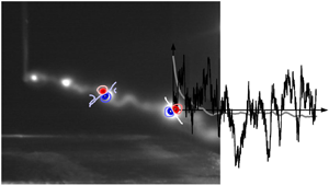
A snapshot of the meandering vortex in a smoke visualisation realised in another facility by T. Leweke (CNRS-IRPHE, Marseille, France) is shown in figure 1 for illustration. In this perspective view, the vortex, corresponding to the light-grey tubular structure, is generated on the left-hand side and propagates to the right, out of the plane. Meandering denotes the clearly visible lateral displacement of the vortex, thus requiring two independent variables for its characterisation in a fixed measurement plane. The erratic nature of the vortex motion suggests modelling meandering as a bivariate random process, which, provisionally, we refer to as  $x_i(t)$,
  $i=1,2$, deferring the definition to § 2.3.

Figure 1. Smoke visualisation of vortex meandering in an experiment (image courtesy Thomas Leweke, IRPHE-CNRS, Marseille, France) and the associated universal principal characteristics in a fixed measurement plane. The variance of the streamwise vorticity component is progressively concentrated in a pair of dipolar patterns (leading proper orthogonal decomposition modes  $\hat {\phi }_i(\boldsymbol {r})$,
  $i = 1,2$). A sample of the associated principal component
  $x_i(t)$ over the measurement time
  $t$ is shown by a black line (arbitrary scaling). These time series are empirically Gaussian distributed
  $\hat {f}_{X_i}(x_i)$ and have approximately exponential autocorrelation
  $\hat {\rho }_{ii}(\tau ) \approx \exp (-\hat {\lambda }_i \tau )$, where
  $\hat {\lambda }_i$ denotes the estimated reciprocal vortex response time.
It is generally admitted that vortex meandering is associated with the energy-carrying, slow scales of the vortex dynamics (Devenport et al. Reference Devenport, Rife, Liapis and Follin1996; Jacquin et al. Reference Jacquin, Fabre, Geffroy and Coustols2001; Roy & Leweke Reference Roy and Leweke2008; Bailey et al. Reference Bailey, Pentelow, Ghimire, Estejab, Green and Tavoularis2018; Bölle Reference Bölle2021). We therefore apply a low-pass filter to  $x_i(t)$ in order to restrict to the governing temporal scales and remove some measurement noise at high frequencies. Inspection of the associated power spectra suggests applying a low-pass filter at a cut-off frequency
  $f_{c} = {300}\ {\rm Hz}$, i.e.
  $f_{c} /f_{s} = 0.1$ compared with the PIV sampling frequency. The corresponding cut-off period is
  $\Delta t_{c} = 1/f_{c} = 3.3\times 10^{-3}\ {\rm s}$, or
  $\Delta t_{c}/\Delta t = 10$ in terms of the PIV sampling period. By the Nyquist–Shannon sampling theorem, this implies the highest resolved frequency
  $f_{r} \leq 0.5 f_{c} = \frac {1}{20}f_{s} = {150}\ {\rm Hz}$, or equivalently, periods longer than
  $\Delta t_{r} \geq 2\,\Delta t_{c} = 20\,\Delta t$.
A characteristic statistical time scale associated with a random process is its integral scale, defined as  $\unicode{x1D4C9}_{I} := \int _0^\infty {\rm d}{\tau } \,\rho (\tau )$, where
  $\rho (\tau )$ denotes the autocorrelation function in (2.5) below (von Storch & Zwiers Reference von Storch and Zwiers2003). In turbulent flows,
  $\unicode{x1D4C9}_{{I}}$ is understood to characterise the energy-carrying, slow scales and should therefore be the pertinent scale for vortex meandering (Tennekes & Lumley Reference Tennekes and Lumley1972). From the experimental data, we estimate
  $\hat {\unicode{x1D4C9}}_{I}/\Delta t \approx 10^2$, i.e. the integral scale dynamics is probed about 100 times. In terms of the low-pass filtered data,
  $\hat {\unicode{x1D4C9}}_{I}/\Delta t_{c} \approx 10$, such that
  $\hat {\unicode{x1D4C9}}_{I}/\Delta t_{r} \approx 5$. We conclude that the energy-carrying processes of the order of the integral scale are resolved in the experiment.
2.2. Review of the relevant elements from the theory of stochastic processes
We recall here some relevant terminology from the theory of stochastic processes; refer to Chandrasekhar (Reference Chandrasekhar1943), Yaglom (Reference Yaglom1962) and de Groot & Mazur (Reference de Groot and Mazur1984) for details.
From our discussion of the experiment in § 2.1, we postulate that vortex meandering is described by the bivariate random process  $t \mapsto X_i(t)$ (
 $i = 1, 2$). If we further assume that vortex meandering is Markovian (cf. §§ 1 and 5), then knowledge of the equilibrium distribution
  $f(\boldsymbol {x})$ and the transition probability
  $f(\boldsymbol {x}_0 \,|\, \boldsymbol {x},t)$ fully characterises the random process. Here, we anticipate that meandering is a stationary process in the measurement time (cf. § 5.3) and assume the existence of an initial state
  $\boldsymbol {x}_0$ such that also the transition probability is stationary (de Groot & Mazur Reference de Groot and Mazur1984). This is, of course, consistent with the expected dynamics of an experiment. We thus define the general stochastic moments
 $$\begin{gather} \overline{g(\boldsymbol{x})}^{eq} = \int_{\mathbb{R}} \text{d}^{2}{x}\, f(\boldsymbol{x})\,g(\boldsymbol{x}) , \end{gather}$$
 $$\begin{gather} \overline{g(\boldsymbol{x})}^{\boldsymbol{x}_{0}}(t) = \int_{\mathbb{R}} \text{d}^{2}{x}\, f(\boldsymbol{x}_0 \,|\, \boldsymbol{x},t)\,g(\boldsymbol{x}) . \end{gather}$$
In particular, the expectation and variance are defined by
 \begin{equation} \mu_i(t) = E(X_i(t)) = \overline{x_i}^{\boldsymbol{x}_{0}}(t) \quad\text{and}\quad \sigma_i^2(t) = V(X_i(t)) = \overline{(x_i - \overline{x_i}^{\boldsymbol{x}_{0}})^2}^{\boldsymbol{x}_{0}}(t) . \end{equation}
 We suppose that the process is stationary in any fixed measurement plane of § 2.1, and introduce the joint distribution function  $F_{X_iX_j}(x_i,x_j;\tau )$,
  $|\tau | \geq 0$, where
  $i,j$ denote any two components of
  $\boldsymbol {X}(t)$ mutually separated by the lag
  $\tau$. Supposing that the two component processes
  $X_i(t)$ and
  $X_j(t)$ (
 $i,j = 1, 2$) have zero expectation, the covariance is defined as
 \begin{equation} C_{ij}(\tau) = E(X_i(t)\,X_j(t+\tau)) = \int_{\mathbb{R}^2} x_ix_j \,{\rm d}{F_{X_iX_j}(x_i,x_j;\tau)} ,\quad |\tau| \geq 0 , \end{equation}
and the cross-correlation follows from normalisation:
 \begin{equation} [-1,1] \ni \rho_{ij}(\tau) = \frac{E(X_i(t)\,X_j(t+\tau))}{\sigma_i \sigma_j} . \end{equation}
The Wiener–Khinchin theorem relates the covariance function (2.4) and the power spectrum  $G_{ij}(\omega )$ in terms of the Fourier transform pair
 \begin{equation} G_{ij}(\omega) = \frac{1}{2{\rm \pi}}\int_\mathbb{R}{{\rm d}}{\tau}\, {\rm e}^{-\text{i}\omega\tau}\,C_{ij}(\tau) ,\quad C_{ij}(\tau) = \int_\mathbb{R}{{\rm d}}{\omega}\, {\rm e}^{\text{i}\omega \tau}\,G_{ij}(\omega) . \end{equation}
2.3. Definition of vortex meandering and kinematic–dynamic equivalence
Meandering denotes the lateral displacement of the vortex core, clearly visible in figure 1, which readily suggests defining vortex meandering as the motion of the vortex centre. To this end, let  $V$ be a subset of the measurement plane that contains the vortex core for all times. Then the vortex centre is defined as (
 $i = 1,2$)
 \begin{equation} r_{{v},i}(t,z) :=
\frac{1}{\varGamma} \int_V\text{d}^{2}{r}\,r_i\,w(t,z,\boldsymbol{r}),
\quad\text{where}\ \varGamma(t,z)
:= \int_V \text{d}^{2}{r}\, w(t,z,\boldsymbol{r})
\end{equation}
\begin{equation} r_{{v},i}(t,z) :=
\frac{1}{\varGamma} \int_V\text{d}^{2}{r}\,r_i\,w(t,z,\boldsymbol{r}),
\quad\text{where}\ \varGamma(t,z)
:= \int_V \text{d}^{2}{r}\, w(t,z,\boldsymbol{r})
\end{equation}
denotes the circulation contained in  $V$, and
  $(t,z) \mapsto w(t,z)$ is the spatiotemporal evolution of the streamwise vorticity component along the measurement section. Equation (2.7a,b) expresses vortex meandering as the kinematic motion of a geometrical point in space.
In order to obtain a dynamic formulation of the problem, we assume that  $(t,z) \mapsto w(t,z)$ is a spatiotemporal random process and apply the Reynolds decomposition
  $w(t,z,\boldsymbol {r}) = \bar{w}^{eq}(\boldsymbol {r}) + w'(t,z,\boldsymbol {r})$ (de Groot & Mazur Reference de Groot and Mazur1984). Here, we assume that the mean vorticity
  $\bar{w}^{eq}(\boldsymbol {r})$ is stationary and homogeneous, and further expand the fluctuation vorticity as
  $w'(t,z) = \sum _{k=1}^\infty x_k(t,z)\,\phi _k(\boldsymbol {r})$, where
  $\phi _k(\boldsymbol {r})$ are the spatial modes obtained from a proper orthogonal decomposition (POD) of the streamwise component of the fluctuation vorticity (details are given in § 5.1). In figure 1, the typical dipolar pattern of these POD modes is shown by the red–blue contour plots, where
  $\phi _1(\boldsymbol {r})$ and
  $\phi _2(\boldsymbol {r})$ are mutually rotated by
  ${90}^{\circ }$ (see also Roy & Leweke Reference Roy and Leweke2008; Edstrand et al. Reference Edstrand, Davis, Schmid, Taira and Cattafesta2016; Karami et al. Reference Karami, Hangan, Carassale and Peerhossaini2019). Recognising the distinct symmetry of the integrals defined in (2.6a,b), we now use this expansion to express the kinematic meandering motion in terms of the leading POD modes
  $\phi _k(\boldsymbol {r})$. A similar approach was first applied by Bölle (Reference Bölle2023) to the respective covariance operators, where also an estimate of the approximation error is derived.
From (2.7b), we see that only vorticity distributions that are symmetric in the Cartesian frame can have a contribution to the circulation, while any skew-symmetric vorticity patterns integrate to zero. Since the mean vorticity field is essentially axisymmetric (Bölle et al. Reference Bölle, Brion, Couliou and Molton2023), to leading order,
 \begin{equation} \varGamma(t,z) = \int_V
\text{d}^{2}{r}\!\left[\overline{w}^{eq}(\boldsymbol{r}) +
\sum_{k=1}^\infty x_k(t,z)\, \phi_k(\boldsymbol{r})\right]
\approx \int_V \text{d}^{2}{r}\, \overline{w}^{eq}(\boldsymbol{r})
= \text{const.}
\end{equation}
\begin{equation} \varGamma(t,z) = \int_V
\text{d}^{2}{r}\!\left[\overline{w}^{eq}(\boldsymbol{r}) +
\sum_{k=1}^\infty x_k(t,z)\, \phi_k(\boldsymbol{r})\right]
\approx \int_V \text{d}^{2}{r}\, \overline{w}^{eq}(\boldsymbol{r})
= \text{const.}
\end{equation} Analogously, the vortex-centre integral (2.7a) is such that only skew-symmetric vorticity distributions can have a non-zero contribution. As recalled previously, we have considerable experimental evidence that the dominant vortex response modes are indeed skew-symmetric with the characteristic dipolar pattern shown in figure 1. We therefore obtain, to leading order ( $i = 1,2$),
 \begin{align} r_{{v},i}(t,z) = \frac{1}{\varGamma}\int_V \text{d}^{2}{r}\,r_i \left[\overline{w}^{eq}(\boldsymbol{r}) + \sum_{k=1}^\infty x_k(t,z)\,\phi_k(\boldsymbol{r})\right] \approx \left[\frac{1}{\varGamma}\int_V \text{d}^{2}{r}\, r_i\,\phi_i(\boldsymbol{r})\right] x_i(t,z) . \end{align}
Without loss of generality, we can take the coordinates  $r_i$ in (2.9) along the principal axes
  $\boldsymbol {e}_1, \boldsymbol {e}_2$, which are aligned with the leading dipolar vortex response modes (see figure 3 below). Due to orthogonality of the POD modes,
  $r_i\phi _k \sim \delta _{ik}$,
  $i,k = 1,2$, and evaluating the last term in brackets in (2.9) gives a constant factor. This shows that
  $r_{{v},i}(t,z) \sim x_i(t,z)$,
  $i = 1,2$, i.e. the experimentally visible meandering motion (cf. figure 1) is proportional to an equivalent meandering motion in the phase space of the fluctuation dynamics. In particular, meandering is, to leading order, confined to the two-dimensional manifold spanned by the leading two POD modes. We verified that this proportionality holds in the experiment (not shown); see also Bölle (Reference Bölle2023, figure 3).
We emphasise that this derivation shows that vortex meandering is indeed associated with the variance-carrying modes (namely the leading POD modes). This was conjectured previously (e.g. Roy & Leweke Reference Roy and Leweke2008; Edstrand et al. Reference Edstrand, Davis, Schmid, Taira and Cattafesta2016; Dghim et al. Reference Dghim, Ben Miloud, Ferchichi and Fellouah2021) and already anticipated in § 2.1, but to the best of the authors' knowledge, has never been shown rigorously (part of the result has already been given in Bölle Reference Bölle2023). Thus, in what follows, we consider the bivariate spatiotemporal random process  $x_i(t,z) = (w'(t,z),\phi _i)$ of principal components. A typical record in a fixed measurement plane at
  $z = \text{const.}$ is shown in figure 1.
2.4. The universal vortex meandering characteristics
Before introducing our theoretical meandering model in § 3, it is instructive to recall the principal meandering characteristics observed universally in experiments. Therewith, we pursue the twofold objective to (i) motivate our modelling strategy and (ii) lay down the minimum features that any candidate model must explain. For measurements taken in a fixed plane, these universal meandering characteristics are superposed on the smoke visualisation shown in figure 1 for the sake of illustration.
The identification of vortex meandering with a bivariate random process implies that a full characterisation would, in principle, require knowledge of all finite joint probability distributions (Yaglom Reference Yaglom1962). In practice, we have considerable experimental evidence that the second-order correlation structure already encodes all essential aspects of the phenomenon. In particular, previous studies unanimously suggest the following.
(i) The empirical probability distribution of vortex meandering is close to Gaussian (e.g. Baker et al. Reference Baker, Barker, Bofah and Saffman1974; Devenport et al. Reference Devenport, Rife, Liapis and Follin1996; Bailey & Tavoularis Reference Bailey and Tavoularis2008; Dghim et al. Reference Dghim, Ben Miloud, Ferchichi and Fellouah2021).
(ii) The standard deviation of the vortex-centre position (referred to as meandering amplitude) increases monotonically downstream (e.g. Devenport et al. Reference Devenport, Rife, Liapis and Follin1996; van Jaarsveld et al. Reference van Jaarsveld, Holten, Elsenaar, Trieling and Van Heijst2011; Edstrand et al. Reference Edstrand, Davis, Schmid, Taira and Cattafesta2016).
(iii) The associated leading-order vortex response corresponds to a dipolar fluctuation vorticity pattern approximately confined to the vortex core (e.g. Roy & Leweke Reference Roy and Leweke2008; Edstrand et al. Reference Edstrand, Davis, Schmid, Taira and Cattafesta2016; Karami et al. Reference Karami, Hangan, Carassale and Peerhossaini2019; Bölle et al. Reference Bölle, Brion, Couliou and Molton2023).
(iv) The vortex response has a continuous power spectrum in each measurement plane, with variance levels monotonically increasing towards low frequencies (e.g. Devenport et al. Reference Devenport, Rife, Liapis and Follin1996; Bailey & Tavoularis Reference Bailey and Tavoularis2008; Bölle Reference Bölle2023). Equivalently, the estimated autocorrelation functions
 $\hat {\rho }_{ii}(\tau )$, shown in grey in figure 1, approximately follow an exponential autocorrelation function $\rho _{ii}(\tau ) = \exp (-\lambda _i \tau )$, where $\lambda _i$ denotes the reciprocal vortex response time.


While the importance of (some of) these features for the characterisation of vortex meandering was realised repeatedly (Baker et al. Reference Baker, Barker, Bofah and Saffman1974; Devenport et al. Reference Devenport, Rife, Liapis and Follin1996; Jacquin et al. Reference Jacquin, Fabre, Geffroy and Coustols2001; van Jaarsveld et al. Reference van Jaarsveld, Holten, Elsenaar, Trieling and Van Heijst2011; Edstrand et al. Reference Edstrand, Davis, Schmid, Taira and Cattafesta2016), it seems that Bölle (Reference Bölle2021) was the first to explicitly state that these characteristics are the typical signature of a Brownian motion (Chandrasekhar Reference Chandrasekhar1943; de Groot & Mazur Reference de Groot and Mazur1984). To the best of the authors' knowledge, the first attempt at formulating a closed theory on this recognition is due to Bölle (Reference Bölle2023).
3. Linear response theory of vortex meandering
In this section, we gradually introduce a linear stochastic model of vortex meandering. First, § 3.1 reviews the basic elements of a linear model approach. While this model still allows for very different mechanisms, we argue in § 3.2 that some can be precluded on experimental facts. On account of the phenomenology, we propose a conceptual meandering model in § 3.3, and derive characteristics that can be compared against experiments in § 3.4.
3.1. Derivation of a linear model of vortex meandering
Principally, the entire state of the system (vortex) is described by the generic dynamical variable  $\boldsymbol {q}(t,z,\boldsymbol {r})$, for which the Reynolds decomposition
  $\boldsymbol {q}(t,z,\boldsymbol {r}) = \bar{\boldsymbol{q}}^{eq}(\boldsymbol {r}) + \boldsymbol {q}'(t,z,\boldsymbol {r})$ holds. As we are interested in only one particular aspect of the system dynamics (namely that associated with the meandering motion), we implicitly restrict to the pertinent submanifold of the dynamical variables. We then assume that, at least within this manifold, the dynamical variables obey a linear evolution equation of the form
 \begin{equation} \frac{\partial\boldsymbol{q}'}{\partial t} + U_\infty\,\frac{\partial \boldsymbol{q}'}{\partial z} = \boldsymbol{\mathsf{L}}\boldsymbol{q}' + \boldsymbol{\xi} , \end{equation}
subject to initial and boundary conditions. In (3.1),  $\boldsymbol{\mathsf{L}} = \boldsymbol{\mathsf{L}}[\bar{\boldsymbol{q}}^{eq},\boldsymbol {\nabla },R]$ denotes the symbolic linearised Navier–Stokes operator evaluated at the vortex mean state
  $\bar{\boldsymbol{q}}^{eq}$ and parametrised by the Reynolds number
  $R$. The forcing
  $\boldsymbol {\xi }$ represents the integral effect of the second-order nonlinear fluctuation dynamics, which is essentially localised in the free stream surrounding the vortex.
In our discussion so far, we have argued that the meandering dynamics corresponds to the spatiotemporal transport  $(t,z) \mapsto x_i(t,z)$, which suggests the separation ansatz
  $\boldsymbol {q}'(t,z,\boldsymbol {r}) = a(t,z)\,\hat {\boldsymbol {q}}(\boldsymbol {r})$ of the corresponding dynamical variables. Then
  $x_i[\hat {\boldsymbol {q}}](t,z)$ is a function of the dynamical field
  $\hat {\boldsymbol {q}}(\boldsymbol {r})$ in the measurement plane.
Equation (3.1) corresponds to a description of the dynamics in a lab-fixed frame of reference. By the method of characteristics, we readily obtain the corresponding ordinary differential equation
 \begin{equation} \frac{{\rm d}\boldsymbol{q}^{\prime}}{{\rm d}t} = \boldsymbol{\mathsf{L}}\boldsymbol{q}' + \boldsymbol{\xi} ,\quad \boldsymbol{q}'(0) = \boldsymbol{q}_0 , \end{equation}
where the initial condition is supposed to be a sure event (Chandrasekhar Reference Chandrasekhar1943; de Groot & Mazur Reference de Groot and Mazur1984). Equations (3.2a,b) describe the vortex meandering dynamics as seen by a co-moving observer along the ray  $z - U_\infty t = z_0$. This coordinate transform is corroborated by the finding that Taylor's hypothesis holds for vortex meandering perturbations (Jacquin et al. Reference Jacquin, Fabre, Geffroy and Coustols2001).
Equations (3.2a,b) forms a vector-valued Cauchy problem. Its solution  $t \mapsto \boldsymbol {q}'(t)$,
  $\boldsymbol {q}'(t) \in L^2(M)$ for all
  $t$, traces a trajectory in the function space of spatial distributions of the dynamical variable in the measurement plane
  $M$ released from the definite initial state
  $\boldsymbol {q}_0$. The space of square-integrable functions
  $L^2(M)$ is endowed with the inner product
  $(\boldsymbol {f},\boldsymbol {g}) := \int _M\text{d}^{2}{r} \sum _i f_i(\boldsymbol {r})\,g_i^*(\boldsymbol {r})$, with induced norm
  $\|\boldsymbol {f}\| := \sqrt {(\boldsymbol {f},\boldsymbol {f})}$.
Denoting by  $\boldsymbol{\mathsf{L}}^*$ the formal adjoint to
  $\boldsymbol{\mathsf{L}}$ with respect to the inner product, the respective eigenvalue problems read
 \begin{equation} \boldsymbol{\mathsf{L}}\boldsymbol{u}_i = \lambda_i\boldsymbol{u}_i \quad\text{and}\quad \boldsymbol{\mathsf{L}}^*\boldsymbol{v}_i = \lambda_i^*\boldsymbol{v}_i , \end{equation}
where bi-orthogonality  $(\boldsymbol {v}_i,\boldsymbol {u}_j) = (\boldsymbol {v}_i,\boldsymbol {u}_i)\,\delta _{ij}$ holds. While principally we expect the eigenmodes to form a complete set to expand the linear vortex dynamics (Fabre et al. Reference Fabre, Sipp and Jacquin2006; Roy & Subramanian Reference Roy and Subramanian2014), we assume that the meandering motion is represented by
  $n$ relevant eigenmodes, in particular. Thus, we introduce the eigenvalue and eigenmode matrices
  $\varLambda _{ij} = \lambda _i\delta _{ij}$ and
  $\boldsymbol{\mathsf{U}} = [\boldsymbol {u}_1, \boldsymbol {u}_2, \ldots, \boldsymbol {u}_n]$,
  $\boldsymbol{\mathsf{V}} = [\boldsymbol {v}_1, \boldsymbol {v}_2, \ldots, \boldsymbol {v}_n]$. Using the eigenmode expansion
  $\boldsymbol {q}'(t) = \sum _{j=1}^n a_j(t)\,\boldsymbol {u}_j$ in (3.3a,b) yields
 \begin{equation} \frac{{\rm d}\boldsymbol{a}}{{\rm d}t} = \boldsymbol{\varLambda}\boldsymbol{a} + \boldsymbol{f} ,\quad \boldsymbol{a}(0) = \boldsymbol{a}_0 , \end{equation}
upon projection onto the corresponding adjoint eigenmodes, where  $f_j(t) := (\boldsymbol {v}_j,\boldsymbol {\xi }(t))$ and
  $a_{0,j} = (\boldsymbol {v}_j,\boldsymbol {q}_0)$. The general solution of (3.4a,b) reads
 \begin{equation} \boldsymbol{a}(t) - {\rm e}^{t\boldsymbol{\varLambda}}\,\boldsymbol{a}_0 = {\rm e}^{t\boldsymbol{\varLambda}} \int_0^t{\rm d}{s}\,{\rm e}^{-s\boldsymbol{\varLambda}}\,\boldsymbol{f}(s) , \end{equation}
describing the dynamics in the manifold spanned by the  $n$ relevant eigenmodes. The corresponding evolution in physical space readily follows from expansion in the respective eigenmodes,
 \begin{equation} \boldsymbol{q}'(t) - \boldsymbol{\mathsf{U}}\,{\rm e}^{t\boldsymbol{\varLambda}}\,\boldsymbol{a}_0 = \boldsymbol{\mathsf{U}}\,{\rm e}^{t\boldsymbol{\varLambda}} \int_0^t{{\rm d}}{s}\,{\rm e}^{-s\boldsymbol{\varLambda}}\,\boldsymbol{f}(s) . \end{equation}
 Unlike this description of the dynamics in terms of eigenmodes, its characterisation in experiments is in terms of POD modes (see § 2). Alternative modal descriptions, e.g. by dynamic mode decomposition (Gutierrez-Castillo et al. Reference Gutierrez-Castillo, Garrido-Martin, Bölle, García-Ortiz, Aguilar-Cabello and del Pino2022), are only recent to the best of the authors' knowledge. We notice that the combined analysis in terms of POD and eigenmodes is a common approach (de Groot & Mazur Reference de Groot and Mazur1984). Projection of (3.6) onto the  $i$th POD mode
  $\phi _i$ yields
 $$\begin{gather} (\boldsymbol{\phi}_i,\boldsymbol{q}'(t)) = \boldsymbol{\phi}_i^*\boldsymbol{\mathsf{U}}\,{\rm e}^{t\boldsymbol{\varLambda}} \left[ \boldsymbol{a}_0 + \int_0^t{{\rm d}}{s}\,{\rm e}^{-s\boldsymbol{\varLambda}}\,\boldsymbol{f}(s) \right] \end{gather}$$
 $$\begin{gather}\iff\quad x_i(t) = \sum_{j=1}^n (\boldsymbol{\phi}_i,\boldsymbol{u}_j)\, {\rm e}^{t\lambda_j} \left[ (\boldsymbol{v}_j,\boldsymbol{q}_0) + \int_0^t{\rm d}{s}\, {\rm e}^{-s\lambda_j}\,(\boldsymbol{v}_j,\boldsymbol{\xi}(s)) \right] . \end{gather}$$
Equation (3.8) identifies two general processes that contribute, in principle, to experimentally observed vortex meandering  $x_i(t)$, namely (i) the amplification of initial perturbations and (ii) sustained forcing. Furthermore, since the eigenmodes
  $\boldsymbol {u}_j$ are not orthogonal, there will, in general, be several with non-null projection onto the
  $i$th POD mode. Thus, principally very different mechanisms may result in a practically identical, experimentally indistinguishable vortex response. Analyses of the different modal and non-modal growth mechanisms have been the subject of numerous previous studies (e.g. Antkowiak & Brancher Reference Antkowiak and Brancher2004; Fabre et al. Reference Fabre, Sipp and Jacquin2006; Fontane, Brancher & Fabre Reference Fontane, Brancher and Fabre2008; Hussain, Pradeep & Stout Reference Hussain, Pradeep and Stout2011; Mao & Sherwin Reference Mao and Sherwin2012; Edstrand et al. Reference Edstrand, Davis, Schmid, Taira and Cattafesta2016; Viola, Arratia & Gallaire Reference Viola, Arratia and Gallaire2016; Bölle et al. Reference Bölle, Brion, Robinet, Sipp and Jacquin2021; Qiu et al. Reference Qiu, Cheng, Xu, Xiang and Liu2021). The important point to be made here is that all these different approaches identify the same dipolar response pattern observed experimentally, yet by different physical mechanisms. Hence, which mechanism was operational in a particular experiment cannot be decided principally by solely inspecting the vortex response expanded in POD modes.
To the best of the authors' knowledge, which interaction pair  $\{\boldsymbol {u}_i,\boldsymbol {v}_i\}$ is the most relevant in the experiment cannot be decided at present. Optimal forcing structures found in theory typically carry several orders of magnitude less energy than the associated response patterns, which makes their detection with standard tools focusing on variance-governing modes (such as POD) difficult. Furthermore, they usually have a fine-grained, filament-like spatial structure that is not resolved in experiments, and even if it were, there is no reason to expect actually realised forcing to resemble the theoretical optimal. In fact, this is not even needed, since already a non-zero projection suffices. It is, however, possible to reject some mechanisms a posteriori, since the dynamical consequences are experimentally not observed.
At this point, it is convenient to pause our development of the meandering model to discuss the possible mechanisms. This will provide orientation about the next steps, as we can exclude some mechanisms on the basis of experimental evidence.
3.2. Discussion of the candidate mechanisms
In retrospect, it appears that previous attempts at explaining vortex meandering concentrated on only some of the universal characteristics identified in § 2.4. Early studies, emphasising the Gaussian distribution and broadband spectral signature, concluded that meandering is essentially the consequence of an ‘inactive vortex being beaten by the surrounding turbulence’ (e.g. Baker et al. Reference Baker, Barker, Bofah and Saffman1974; Devenport et al. Reference Devenport, Rife, Liapis and Follin1996), much like a ‘passive tracer’ (van Jaarsveld et al. Reference van Jaarsveld, Holten, Elsenaar, Trieling and Van Heijst2011). On the other hand, already Bandyopadhyay et al. (Reference Bandyopadhyay, Stead and Ash1991) emphasised the ‘dynamic nature’ of the vortex, suggesting that meandering is not ‘purely an artefact of the wind-tunnel environment’ (Edstrand et al. Reference Edstrand, Davis, Schmid, Taira and Cattafesta2016). Rather, it was suggested that meandering should be the consequence of an instability (e.g. Jacquin et al. Reference Jacquin, Fabre, Geffroy and Coustols2001; Edstrand et al. Reference Edstrand, Davis, Schmid, Taira and Cattafesta2016; Qiu et al. Reference Qiu, Cheng, Xu, Xiang and Liu2021). This shift in modelling paradigm was accompanied (or caused) by a change of the emphasised meandering characteristics to an exclusive consideration of the downstream amplitude growth and the dipolar vortex response pattern (cf. § 2.4).
The basic argument in favour of an instability mechanism is founded on the recognition that the leading POD mode pair, the fractional variance of which grows monotonically downstream, closely resembles eigenmodes found in stability analyses (Edstrand et al. Reference Edstrand, Davis, Schmid, Taira and Cattafesta2016). Our above derivation (cf. (3.8)) implies that this conclusion cannot actually be drawn from the mere comparison of POD and eigenmodes. Even more, we are not aware of any vortex meandering experiment providing convincing evidence for the existence of an instability (Jacquin et al. Reference Jacquin, Fabre, Geffroy and Coustols2001; Fabre & Jacquin Reference Fabre and Jacquin2004; Bailey & Tavoularis Reference Bailey and Tavoularis2008; Edstrand et al. Reference Edstrand, Davis, Schmid, Taira and Cattafesta2016; Bölle et al. Reference Bölle, Brion, Couliou and Molton2023). This provides strong evidence that experimentally realised, isolated line vortices are in fact stable, and that we have to reject instability sensu stricto as the underlying mechanism.
Staying with the homogeneous solution in (3.8), it was conjectured that vortex meandering may be the consequence of transient growth (e.g. Fabre & Jacquin Reference Fabre and Jacquin2004; Roy & Leweke Reference Roy and Leweke2008; Mao & Sherwin Reference Mao and Sherwin2012; Lee & Marcus Reference Lee and Marcus2024). Largely independent of the Reynolds number, Antkowiak & Brancher (Reference Antkowiak and Brancher2004) show that the time  $\unicode{x1D4C9}_{opt}$ required to reach the optimal amplification by a transient-growth mechanism is of the order of ten rotation periods. That is,
  $\unicode{x1D4C9}_{opt}/\unicode{x1D4C9}_{{r}} \sim 10$, where
  $\unicode{x1D4C9}_{{r}} := 2{\rm \pi} \unicode{x1D4C1}^2\varGamma _\infty ^{-1}$ denotes the rotation time scale. Further defining the advection time scale
  $\unicode{x1D4C9}_{{a}} := cU_\infty ^{-1}$, we readily estimate
  $\unicode{x1D4C9}_{opt}/\unicode{x1D4C9}_{{a}} \sim 1$ with the estimated ratio
  $\unicode{x1D4C9}_{{r}} /\unicode{x1D4C9}_{{a}} \sim 10^{-1}$. This estimation suggests that transient growth operates over a downstream distance of the order of one chord length, contrary to the monotonic amplitude growth over downstream ranges of the order of at least ten chord lengths in experiments (Devenport et al. Reference Devenport, Rife, Liapis and Follin1996; Bailey & Tavoularis Reference Bailey and Tavoularis2008; van Jaarsveld et al. Reference van Jaarsveld, Holten, Elsenaar, Trieling and Van Heijst2011; Bölle et al. Reference Bölle, Brion, Couliou and Molton2023).
Eventually, we note that this estimation is consistent with the experiment of Bailey et al. (Reference Bailey, Pentelow, Ghimire, Estejab, Green and Tavoularis2018), who speculated that the vortex response may have contributions from transient growth in their first measurement plane, albeit their experiment suggests that transient growth, even if it persisted afterwards, seemed overwhelmed by other mechanisms and was not clearly discernible for increased free-stream turbulence intensity. Therefore, while transient growth is likely not the governing mechanism of vortex meandering, the results nevertheless suggest that the underlying mechanism plays a role in experimental vortex dynamics.
We have considerable experimental evidence that changes in the intensity of the free-stream turbulence (e.g. grid turbulence) affect vortex meandering quantitatively rather than qualitatively (van Jaarsveld et al. Reference van Jaarsveld, Holten, Elsenaar, Trieling and Van Heijst2011; Bailey et al. Reference Bailey, Pentelow, Ghimire, Estejab, Green and Tavoularis2018). That is, enhanced free-stream turbulence intensities increase the meandering strength, but seem not to affect the principal characteristics. This suggests that meandering may be the result of some resonance mechanism, in which the vortex constitutes a self-stabilising entity that is continuously excited by the surrounding free-stream turbulence. The stabilising intrinsic vortex dynamics is associated with (Kelvin) waves propagating along the vortex core (Jacquin et al. Reference Jacquin, Fabre, Geffroy and Coustols2001; Fabre & Jacquin Reference Fabre and Jacquin2004). In fact, very likely both aspects – sustained external forcing and intrinsic, stabilising vortex dynamics – are relevant (Bandyopadhyay et al. Reference Bandyopadhyay, Stead and Ash1991; Fontane et al. Reference Fontane, Brancher and Fabre2008; Bailey et al. Reference Bailey, Pentelow, Ghimire, Estejab, Green and Tavoularis2018).
Generally, the most important contribution to (3.8) will be from those perturbations that together maximise the different projections and are not too strongly damped. Theoretical studies indicate the existence of two near-neutral eigenmode families, referred to as D and L1 by Fabre et al. (Reference Fabre, Sipp and Jacquin2006), for which the vortex response pattern visually resembles the leading POD mode. While the displacement (D) waves are associated with an effectively normal linear operator, critical-layer (L1) waves are at the heart of the non-normal dynamics (Antkowiak & Brancher Reference Antkowiak and Brancher2004; Fontane et al. Reference Fontane, Brancher and Fabre2008; Bölle et al. Reference Bölle, Brion, Robinet, Sipp and Jacquin2021). On account of our discussion, we assume that vortex meandering is essentially governed by a critical-layer dynamics. Thence, supposing a single governing mode  $j$, introducing the shorthand identifications
  $x_{0,i} \leftarrow (\phi _i,\boldsymbol {u}_j)(\boldsymbol {v}_j,\boldsymbol {q}_0)$ and
  $f_i(t) \leftarrow (\phi _i,\boldsymbol {u}_j)(\boldsymbol {v}_j,\boldsymbol {f}(t))$, (3.8) simplifies to
 \begin{equation} x_i(t) - {\rm e}^{t\lambda_i}\,x_{0,i} = {\rm e}^{t\lambda_i}\int_0^t{{\rm d}}{s}\, {\rm e}^{-s\lambda_i}\,f_i(s) \quad (i = 1,2) , \end{equation}
where we have used the experimental evidence that meandering is associated with the leading two POD modes (§ 2.3).
From the stability analysis of Fabre et al. (Reference Fabre, Sipp and Jacquin2006), we estimate that a characteristic vortex response time scale  $\unicode{x1D4C9}_{{s}} = \lambda _i^{-1}$ should to be of the order of
  $\unicode{x1D4C9}_{{s}} /\unicode{x1D4C9}_{{r}} \sim 10^2$. With our above scale estimates, we readily obtain
  $\unicode{x1D4C9}_{{s}} /\unicode{x1D4C9}_{{a}} \sim 10$, in agreement with our previous conclusions.
3.3. Phenomenology and conceptual vortex meandering model
In order to frame vortex meandering in the concepts of statistical mechanics, we start from an abstraction of the general experimental set-up outlined in § 2.1. To a first approximation, we may consider the experimental configuration as consisting of an isolated vortex evolving in a (weakly) turbulent free stream. In the language of statistical mechanics, we identify the vortex with our system, and refer to the free-stream turbulence as a heat bath. The intensity of the heat bath will be given by the free-stream turbulence intensity  $\unicode{x1D4CA}$ of the empty facility.
As a qualitative model of the heat bath, we may imagine the free-stream turbulence filling the wind tunnel to be an assembly of a very large number of small-scale vortices, evolving rapidly over a very short time scale  $\unicode{x1D4C9}_{{f}}$. We therefore assume that the free-stream turbulence has no particular spatial or temporal structure, thus being characterised by stationary and homogeneous statistics. Putting the large-scale vortex in the heat bath, we think of the small-scale vortices exerting minute excitations in very rapid succession. While we do not know the details of each elementary excitation, slow (scale
  $\unicode{x1D4C9}_{{s}}$) reactions of the large-scale vortex integrate over time. This essentially corresponds to a Brownian motion – where each elementary excitation is highly complicated and unobserved, the integral effect of very many minute events accumulates to a macroscopic and visible effect, manifest in figure 1.
On account of this phenomenology, we assume that the time scale separation  $\unicode{x1D4C9}_{{s}} \gg \unicode{x1D4C9}_{{f}}$ holds between the characteristic scales of the large-scale vortex and the surrounding small-scale turbulence. Then on the slow time scale
  $\unicode{x1D4C9}_{{s}}$, the forcing approximately corresponds to a white noise process, with
 \begin{equation} \bar{f}_{i}^{\boldsymbol{x}_{0}}(t) = 0 ,\quad \overline{f_i(s)\,f_j(t)}^{\boldsymbol{x}_{0}} = 2B_{ij}\,\delta(t-s) \quad (i,j = 1,2), \end{equation}
where  $B_{ij}$ determines the strength and mutual correlation of the forcing. With this additional assumption on the forcing statistics, (3.4a,b) corresponds to a Langevin equation, while its solution (3.5) (or (3.9)) is known as an Ornstein–Uhlenbeck process, describing a Brownian motion (Chandrasekhar Reference Chandrasekhar1943; Yaglom Reference Yaglom1962; de Groot & Mazur Reference de Groot and Mazur1984). We emphasise that consequently, framing vortex meandering as a problem in stochastic mechanics contains both previous explanation families (cf. § 1) as limiting cases. Linear deterministic dynamics results as the external fluctuations asymptotically tend to zero, while a purely externally driven dynamics would be the consequence of a vanishing intrinsic vortex resistance.
3.4. Non-equilibrium dynamics of the Langevin system
Equations (3.9)–(3.10) summarise our final vortex meandering model, taking the form of a Langevin equation. In the following, we derive characteristic model properties that can be evaluated statistically in experiments. The relevant methodology for this purpose will be introduced in § 4.
3.4.1. Gaussian probability distribution
Our assumption of time scale separation implies the existence of an intermediate time increment  $\Delta t$ such that
  $\unicode{x1D4C9}_{{f}} \ll \Delta t \ll \unicode{x1D4C9}_{{s}}$. We can then expand the particular solution as
 \begin{align} \boldsymbol{x}(t) - {\rm e}^{t\boldsymbol{\varLambda}}\,\boldsymbol{x}_0 &= {\rm e}^{t\boldsymbol{\varLambda}} \int_0^t{{\rm d}}{s}\,{\rm e}^{-s\boldsymbol{\varLambda}}\, \boldsymbol{f}(s) = {\rm e}^{t\boldsymbol{\varLambda}} \sum_{k=0}^{K-1} \int_{k\,\Delta t}^{(k+1)\, \Delta t}{{\rm d}}{s} \,{\rm e}^{-s\boldsymbol{\varLambda}}\,\boldsymbol{f}(s) \nonumber\\ &\approx \sum_{k=0}^{K-1} {\rm e}^{(t-k\,\Delta t)\boldsymbol{\varLambda}} \int_{k\,\Delta t}^{(k+1)\,\Delta t}{{\rm d}}{s} \,\boldsymbol{f}(s) = \sum_{k=0}^{K-1} {\rm e}^{(t-k\,\Delta t)\boldsymbol{\varLambda}}\,\boldsymbol{W}(\Delta t) . \end{align}
Here, we have used that due to time scale separation, the exponential function is practically constant over the time increment. Formally, (3.11) expresses meandering as a random walk, where each ‘step’  $\boldsymbol {W}(\Delta t)$ of the vortex is the integral over a succession of a great many minute excitations,
  $\int _{k\,\Delta t}^{(k+1)\,\Delta t}{{\rm d}}{s} \,\boldsymbol {f}(s)$. Thus, the slow vortex fluctuation dynamics is the sum over a large number
  $K \gg 1$ of independent, identically distributed excitation events. By the central limit theorem, we therefore conclude that the vortex dynamics must have a Gaussian distribution (Chandrasekhar Reference Chandrasekhar1943, Lemma I on p. 23).
3.4.2. Two-point statistics in evolution time
If meandering corresponds to a Markov process, we further need to specify the correlation structure to obtain a complete classification of the stochastic dynamics.
Taking the mean of (3.9) for a trajectory started from a definite initial perturbation yields
 \begin{equation} \bar{\boldsymbol{x}}^{\boldsymbol{x}_{0}}(t) = {\rm e}^{t\boldsymbol{\varLambda}}\,\boldsymbol{x}_0 \end{equation}
on account of the forcing statistics (3.10). Equation (3.12) is formally identical to the homogeneous solution of the associated deterministic problem, and as such, subject to the linear-stability and transient-growth studies discussed in § 3.2. That is, in a systematically stochastic theory, practically deterministic dynamics is an approximation valid in the limit of a sharp transition probability density  $f(\boldsymbol {x}_0 \,|\, \boldsymbol {x},t)$ (de Groot & Mazur Reference de Groot and Mazur1984).
The leading-order variability around the mean trajectory (3.12) is given by the covariance
 \begin{equation} \boldsymbol{\mathsf{C}}(t) = \overline{(\boldsymbol{x} - \bar{\boldsymbol{x}}^{\boldsymbol{x}_{0}})(\boldsymbol{x} - \bar{\boldsymbol{x}}^{\boldsymbol{x}_{0}})^*}^{\boldsymbol{x}_{0}}(t) = 2\int_0^t {{\rm d}}{s}\,{\rm e}^{(t-s)\boldsymbol{\varLambda}}\, \boldsymbol{\mathsf{B}}\,{\rm e}^{(t-s)\boldsymbol{\varLambda}^*} . \end{equation}
Further, let  $\boldsymbol{\mathsf{C}}^{{eq}}$ be the covariance associated with the equilibrium probability distribution. Then the competition between sustained stochastic excitation by the surrounding free stream and the intrinsically stabilising vortex dynamics (cf. § 3.2) implies asymptotic convergence,
  $\boldsymbol{\mathsf{C}}^{{eq}} = \boldsymbol{\mathsf{C}}(t \to \infty )$. The fluctuation–dissipation theorem (de Groot & Mazur Reference de Groot and Mazur1984)
 \begin{equation} \boldsymbol{\varLambda}\boldsymbol{\mathsf{C}}^{{eq}} + \boldsymbol{\mathsf{C}}^{{eq}}\boldsymbol{\varLambda}^* = 2\boldsymbol{\mathsf{B}} \end{equation}
uniquely relates the equilibrium covariance of the vortex response to the intensity of the exciting turbulence. A POD of the fluctuation–dissipation theorem (3.14) is the subject of stochastic forcing analyses (Farrell & Ioannou Reference Farrell and Ioannou1996; Fontane et al. Reference Fontane, Brancher and Fabre2008).
For the particular case of modal dynamics (3.9), the components of (3.13) uncouple and we obtain the variance evolution
 \begin{equation} \sigma_i^2(t) = \overline{(x_i - \bar{x}_i^{\boldsymbol{x}_{0}})^2}^{\boldsymbol{x}_{0}}(t) \sim \unicode{x1D4CA}^2\left( 1 - {\rm e}^{2\lambda_i t} \right) \quad (i = 1,2) \end{equation}
upon setting  $B_{ij} \sim \unicode{x1D4CA}^2\,\delta _{ij}$ (Bölle Reference Bölle2023). For
  $t$ of the order of the vortex response time
  $\unicode{x1D4C9}_{{s}} = \lambda _i^{-1}$, we approximate (3.15) by its leading-order expansion (Bölle Reference Bölle2023)
 \begin{equation} \sigma_i^2(t) \sim 2\unicode{x1D4CA}^2 \lambda_i t \sim 2\unicode{x1D4CA}^2\,\frac{t}{\unicode{x1D4C9}_{{s}}} . \end{equation}
This law of variance growth was proposed on phenomenological reasoning by van Jaarsveld et al. (Reference van Jaarsveld, Holten, Elsenaar, Trieling and Van Heijst2011), and found to hold for other experiments (Bailey et al. Reference Bailey, Pentelow, Ghimire, Estejab, Green and Tavoularis2018; Bölle Reference Bölle2021, Reference Bölle2023).
3.4.3. Two-point statistics in measurement time
By design, we expect experiments to have reached stationarity when performing measurements (cf. § 5.3). Measurement sequences in fixed planes (at  $z = \text{const.}$) are then amenable to Fourier analysis. For the Langevin model (3.9)–(3.10), the equilibrium autocovariance function and power spectrum read (Yaglom Reference Yaglom1962; von Storch & Zwiers Reference von Storch and Zwiers2003)
 \begin{equation} C_{ii}(\tau) = \sigma_i^2\,{\rm e}^{-\lambda_i\,|\tau|} \quad\text{and}\quad G_{ii}(\omega) = \frac{\sigma_i^2\lambda_i}{\rm \pi}\,\frac{1}{\lambda_i^2 + \omega_i^2} \quad (i = 1,2). \end{equation}
 We recall that our Brownian motion vortex meandering model is essentially parametrised by two variables,  $\unicode{x1D4CA}$ and
  $\unicode{x1D4C9}_{{s}}$, measuring the strength of the surrounding turbulence and the vortex response time scale, respectively. This is in agreement with the findings of van Jaarsveld et al. (Reference van Jaarsveld, Holten, Elsenaar, Trieling and Van Heijst2011) and Bailey et al. (Reference Bailey, Pentelow, Ghimire, Estejab, Green and Tavoularis2018), who assumed that
  $\unicode{x1D4C9}_{{s}}$ was given by the vortex rotation time scale
  $\unicode{x1D4C9}_{{r}}$. In § 3.1, we show that
  $\unicode{x1D4C9}_{{s}}$ is related to the eigenvalues of the linearised vortex dynamics, and more specifically, argue in § 3.2 that vortex meandering may likely be associated with critical-layer vortex waves. Hence, in principle,
  $\unicode{x1D4C9}_{{s}}$ can be determined if the vortex mean flow and the external flow parameters (e.g. Reynolds number) are known. We have considerable experimental evidence that vortex meandering is directly proportional to the intensity of the surrounding turbulence but not affected by its spectral signature (Bailey & Tavoularis Reference Bailey and Tavoularis2008; van Jaarsveld et al. Reference van Jaarsveld, Holten, Elsenaar, Trieling and Van Heijst2011; Bailey et al. Reference Bailey, Pentelow, Ghimire, Estejab, Green and Tavoularis2018; Dghim et al. Reference Dghim, Ben Miloud, Ferchichi and Fellouah2021). This is reflected in the model proposed here. Thus, the formulae of this section could in principle also be used to predict vortex meandering, provided that the vortex mean flow, the Reynolds number and the turbulence intensity are known. These predictions should capture the right qualitative behaviour; however, a quantitatively correct prediction of the meandering motion would require scaling terms of order unity omitted here (cf. §§ 3.1–3.2 and Bölle Reference Bölle2023).
4. Statistical inference: relating theory and experiment
So far in this study, we have disposed of two descriptive elements for the phenomenon of vortex meandering, namely (i) the mathematical model introduced in § 3, and (ii) an experiment relative to the phenomenon in question (cf. § 2). While at the outset these two elements pertain to entirely different spheres (Cramér Reference Cramér1963), we derived model characteristics in § 3.4 that can be estimated in experiments. Statistical inference provides the theoretical frame and tools to assess given statistical data in the context of the adopted model. This, principally, gives us the possibility of confirming or rejecting our model on an objective and reproducible statistical basis.
4.1. Sampling
For the purpose of this study, we formally identify the wind tunnel experiment with a random experiment  $\mathfrak {E}$. One realisation of
  $\mathfrak {E}$ corresponds to a spatial meandering trajectory
  $z \mapsto X^{(t)}(z)$, drawn at random from the totality of all admissible meandering paths (called the population). In this sense, the snapshot shown in figure 1 for some time instant
  $t$ represents one such realisation of
  $\mathfrak {E}$. Keeping the experimental conditions fixed and running the wind tunnel experiment over a certain time
  $T$, while recording the outcomes at the rate
  $\Delta t$, corresponds conceptually to the repetition of
  $\mathfrak {E}$
  $N = T/\Delta t$ times. The result of one measurement run will be a sequence of particular realisations, all drawn at random from the same probability distribution. This subset of the entire population is called the sample (Cramér Reference Cramér1963). Current experiments do not resolve the downstream meandering trajectory; rather, only samples gathered in a small number of measurement planes at fixed
  $z$ (cf. § 2.1) are experimentally available. Thus, while principally
  $\mathfrak {E}$ corresponds to a function-valued random process, our further analysis is limited to scalar-valued samples. Let us formalise these notions.
Consider a random experiment  $\mathfrak {E}$ connected with a random variable
  $X$ taking values from some parent population,
  $\mathbb {R}$ say, according to the distribution function
  $F_X(x)$. Suppose that we repeat
  $\mathfrak {E}$
  $N$ times; then the outcome of the
  $n$th trial is the actual realisation
  $X^{(n)} = x_n$, where
  $n = 1,2,\ldots,N$. The set of realisations
  $\boldsymbol {x}^{(k)}_N = \{x_1^{(k)},x_2^{(k)},\ldots,x_N^{(k)}\} \subset \mathbb {R}$ is called a random sample. Of course, we could, in theory, repeat the sampling process, i.e. drawing
  $N$ times anew from
  $\mathfrak {E}$, which leads to another equally possible random sample (von Storch & Zwiers Reference von Storch and Zwiers2003). To emphasise the random nature of the sample, we denote the
  $k$th realisation by
  $\boldsymbol {x}^{(k)}_N$. The process of sampling is shown schematically in figure 2(a).

Figure 2. Basic elements of the theory of estimation and hypothesis testing. (a) Schematic of the sampling process for the random variable  $X$ having probability density
  $f_X(x)$ (empirical density
  $\hat {f}_X(x)$). Repetition of the sampling yields a priori different samples
  $\boldsymbol {x}^{(k)}_N$ of the population. (b) The
  $k$th point estimator
  $\hat {\kappa }^{(k)}$ and confidence interval
  $(\hat {\kappa }_{\tilde {p}}^L,\hat {\kappa }_{\tilde {p}}^U)^{(k)}$ of the statistical characteristic
  $\kappa$ with true population value
  $\kappa _0$. The sampling distribution (density
  $f_{\hat {\kappa }}(\kappa )$) determines the variability of the estimator and interval width. The non-rejection region
  $\varTheta (\,\tilde {p}) = (\kappa _{\tilde {p}}^-,\kappa _{\tilde {p}}^+)$ of the null hypothesis
  $H_0: \kappa =\kappa _0$ at the
  $(1-\tilde {p})\times 100\,\%$ significance level is indicated. Schematic test statistics
  $\mathfrak {d}_N^{(k)}$ for different samples illustrate the duality with the confidence intervals.
4.2. Theory of estimation and hypothesis testing
4.2.1. Estimation
Typically, random variables are characterised in terms of statistical characteristics  $\kappa$ (e.g. expectation and variance) taking fixed non-random values
  $\kappa _0$, say. On the other hand, the corresponding sample characteristics (e.g. sample mean and variance) are computed by (nonlinearly) combining the random sample elements
  $x_n^{(k)}$,
  $n = 1,2,\ldots,N$. Therefore, unlike the non-random population characteristics, sample characteristics are again random variables. To discriminate between population and sample characteristics, we adopt the usual convention to denote the
  $k$th estimator of the true characteristic
  $\kappa = \kappa _0$, computed from the
  $k$th sample
  $\boldsymbol {x}^{(k)}_N$, by
  $\hat {\kappa }^{(k)}_N = \hat {\kappa }(\boldsymbol {x}^{(k)}_N)$.
Since  $\hat {\kappa }_N$ is a random variable, a full characterisation requires knowledge of its probability distribution. This sampling distribution
  $F_{\hat {\kappa }}(\kappa )$ is specific to each sample characteristic
  $\hat {\kappa }_N$, and uniquely determined by the distribution function
  $F_X(x)$ (Cramér Reference Cramér1963). In particular, the sampling distribution determines the variability of the associated sample characteristic. This is displayed schematically in figure 2(b), showing the sampling probability density
  $f_{\hat {\kappa }}(\kappa )$ of some arbitrary characteristic along with possible estimates
  $\hat {\kappa }^{(k)}_N$ computed from three different samples
  $\boldsymbol {x}^{(k)}_N$,
  $k = 1,2,3$. This example illustrates that point estimators
  $\hat {\kappa }^{(k)}_N$ will generally be different for each sample and different from the true characteristic
  $\kappa _0$.
We emphasise that the above definition of a sample characteristic as a function of the sample, in principle, allows for an infinite number of candidate estimators. Each estimator is fully determined by its unique sampling distribution, the statistical characteristics of which define the estimator properties and usefulness. In practice, the assessment of the quality of any given estimator is essentially based on the expectation and variance of the estimator. An estimator is called unbiased if its expectation equals the population characteristic, i.e.  $E(\hat {\kappa }_N) = \kappa _0$ for all
  $N$. It is further desirable that estimators are in an as close neighbourhood of the true value as possible. This leads to a definition of the efficiency of an estimator
  $E((\hat {\kappa }_N - \kappa _0)^2) = (E(\hat {\kappa }_N) - \kappa _0)^2 + V(\hat {\kappa }_N)$ as the sum of its squared bias and variance. The objective is to find unbiased and minimum-variance estimators. A systematic approach to obtain estimators is by the maximum likelihood method (Cramér Reference Cramér1963; von Storch & Zwiers Reference von Storch and Zwiers2003).
Our discussion so far makes clear that point estimators are random functions that map given samples on random values. As such, one particular value of the characteristic  $\hat {\kappa }_N^{(k)}$, realised in the experiment
  $\boldsymbol {x}_N^{(k)}$, is of limited significance. Rather, reliable statements require robust estimates of the characteristic that, although obtained from only one sample, have value for all experiments that could have been conducted alternatively. This is the purpose of interval estimators (von Storch & Zwiers Reference von Storch and Zwiers2003). The confidence interval indicates the uncertainty in the estimate that is unavoidable since we are working with a finite sample of the total population. If we were to draw samples again and again ad infinitum, then the confidence intervals would cover the non-random population characteristic
  $\kappa _0$ with a certain a priori percentage
  $\tilde {p}$. In other words, the confidence interval is obtained for the specific sample, and the confidence level
  $\tilde {p}$ indicates its validity for the totality of all samples that could have been obtained alternatively. We see that as with point estimators, confidence intervals (having random endpoints) are again random functions of the sample. This is shown schematically in the lower part of figure 2(b).
4.2.2. Hypothesis testing
Given a set of measurements, namely a sample, we would like to decide if it is consistent with some theoretical model defined a priori. In order to approve or reject agreement, we define representative characteristics  $\kappa$ that we know to take the value
  $\kappa _0$ in the model, and suppose this to be true. That is, we conjecture the null hypothesis
  $H_0: \kappa = \kappa _0$. We then estimate
  $\kappa$ by the corresponding sample characteristic
  $\hat {\kappa }_N$, and compare the result with the postulated true value. Our previous discussion implies that, in general, equality will never hold exactly, even if
  $H_0$ is true, and since
  $\hat {\kappa }_N$ is a random variable, the agreement will be different for each sample that we test for. We therefore have to specify difference thresholds beyond which we reject the model, because the difference between
  $\hat {\kappa }$ and
  $\kappa _0$ is very unlikely to be due to random variability. This suggests the following practical implementation, the essential elements being shown schematically in figure 2(b).
Define a test statistic  $\mathfrak {d}_N = \mathfrak {d}(\boldsymbol {x}_N)$ in the form of a distance measure
  $\mathfrak {d}(\boldsymbol {x}_N) = \text {dist}(\hat {\kappa }_N,\kappa _0)$. This will, in general, be a nonlinear function of the sample
  $\boldsymbol {x}_N$, therefore the test statistic is itself a random variable with a specific sampling distribution. Fix a non-rejection region, i.e. an interval
  $\varTheta (\,\tilde {p}) = (\kappa _{\tilde {p}}^-,\kappa _{\tilde {p}}^+)$ (around the hypothesised true value
  $\kappa _0$) containing
  $\tilde {p}\times 100\,\%$ of the realisations of
  $\mathfrak {d}(\boldsymbol {x}_N)$ when
  $H_0$ is true. The interval is determined by the sampling distribution of the test statistic
  $\mathfrak {d}_N$ (Wilks Reference Wilks2006). The risk
  $(1-\tilde {p})\times 100\,\%$ of falsely rejecting the true null hypothesis is called the significance level, usually set to 5 %–10 % (von Storch & Zwiers Reference von Storch and Zwiers2003). If the actual realisation of the test statistic
  $\mathfrak {d}(\boldsymbol {x}_N)$ falls outside the interval
  $\varTheta (\,\tilde {p})$, then
  $H_0$ is rejected at the
  $(1-\tilde {p})\times 100\,\%$ significance level (Cramér Reference Cramér1963; von Storch & Zwiers Reference von Storch and Zwiers2003; Bendat & Piersol Reference Bendat and Piersol2010).
4.3. The equivalent sample size
In mathematical statistics, sampling means drawing a collection of independent and identically distributed random variables, yielding a set of realisations. Often, in practice, sampling means discretely recording data from a time series. In general, the elements of samples obtained in this way will be correlated, hence the independence assumption fails. In order to be able to use the theoretical results, we assume the sample to be drawn from a stationary, ergodic process (von Storch & Zwiers Reference von Storch and Zwiers2003).
Usually encountered time series have finite correlation (Yaglom Reference Yaglom1962), suggesting that the full sample contains subsets of independent observations (Tennekes & Lumley Reference Tennekes and Lumley1972). Sub-sampling, i.e. considering only sample elements separated by some multiple of the correlation length, therefore would seem to be a simple and straightforward approach to obtain an independent sample from serially correlated data. However, it is known that by this approach, information is lost without improving the estimate (von Storch & Zwiers Reference von Storch and Zwiers2003). Thus, rather than throwing away ‘intermediate’ observations between any two independent elements, we use the full sample and introduce an equivalent sample size based on the autocorrelation structure of the time series (Leith Reference Leith1973; Trenberth Reference Trenberth1984; Thiébaux & Zwiers Reference Thiébaux and Zwiers1984; Zwiers & Von Storch Reference Zwiers and Von Storch1995).
The equivalent sample size is defined as the number of independent random variables needed to provide the same amount of information about the population characteristic as contained in the full sample of dependent variables. As such, the equivalent sample size depends on the characteristic to be tested and how information is measured (Trenberth Reference Trenberth1984; von Storch & Zwiers Reference von Storch and Zwiers2003; Wilks Reference Wilks2006). Letting  $\kappa$ be this characteristic, the number of independent elements in a sample (relative to
  $\kappa$) is defined as
 \begin{equation} N'(\kappa) := \frac{T}{2\,\unicode{x1D4C9}_{{I}}(\kappa)} = \frac{N}{2\,\dfrac{\unicode{x1D4C9}_{{I}}(\kappa)}{\Delta t}},\quad T = N\,\Delta t . \end{equation}
Here,  $T$ denotes the total measurement time of the time series, equal to
  $N\,\Delta t$ if the
  $N$ sample elements are recorded at the constant time step
  $\Delta t$ (cf. § 2.1), and
  $\unicode{x1D4C9}_{{I}} (\kappa )$ is the integral time scale relative to
  $\kappa$. As usual, we refer to twice the integral time scale as the decorrelation time, and write
  $\unicode{x1D4C9}_{{D}} = 2\unicode{x1D4C9}_{{I}}$ (Leith Reference Leith1973; Trenberth Reference Trenberth1984; von Storch & Zwiers Reference von Storch and Zwiers2003).
The decorrelation time for the mean can be estimated in a finite, discrete sample of length  $N$ by (Thiébaux & Zwiers Reference Thiébaux and Zwiers1984; von Storch & Zwiers Reference von Storch and Zwiers2003)
 \begin{equation} \unicode{x1D4C9}_{{D}} \approx \left[1 + 2\sum_{\nu=1}^{N-1} \left(1-\frac{\nu}{N}\right)\rho(\nu)\right] \Delta t \approx \left[1 + 2\sum_{\nu=1}^{N-1} \rho(\nu)\right] \Delta t , \end{equation}
where we assume that  $T \gg \unicode{x1D4C9}_{{I}}$ and that the autocorrelation
  $\rho (\nu )$ decays to zero sufficiently fast as the lag
  $\nu = \tau /\Delta t \to \infty$,
  $\Delta t\neq 0$ (Tennekes & Lumley Reference Tennekes and Lumley1972). Analogously, estimates of the decorrelation time are obtained for other characteristics; in particular,
 $$\begin{gather} \unicode{x1D4C9}_{{D}}
\approx \left[1 + 2\sum_{\nu=1}^{N-1} \rho^2(\nu)\right]
\Delta t \quad \text{for the
variance},
\end{gather}$$
$$\begin{gather} \unicode{x1D4C9}_{{D}}
\approx \left[1 + 2\sum_{\nu=1}^{N-1} \rho^2(\nu)\right]
\Delta t \quad \text{for the
variance},
\end{gather}$$ $$\begin{gather}\unicode{x1D4C9}_{{D}} \approx \left[1 + 2\sum_{\nu=1}^{N-1} \rho_X(\nu)\rho_Y(\nu)\right] \Delta t \quad \text{for the correlation} \end{gather}$$
(see also Bartlett Reference Bartlett1935; Bayley & Hammersley Reference Bayley and Hammersley1946; Trenberth Reference Trenberth1984; von Storch & Zwiers Reference von Storch and Zwiers2003). From (4.2)–(4.4), we see immediately that  $\unicode{x1D4C9}_{{D}} \to \Delta t$ as
  $\rho (\nu ) \to 0$, thus
  $N' \to N$ by (4.1a,b). That is, if it happens that the time series is uncorrelated (i.e. white noise), then the equivalent sample size degenerates to the full sample size. If the time series comes from a first-order autoregressive process, then all the decorrelation – or equivalently, persistence information – is contained in the lag-1 correlation
  $\rho _1 := \rho (\nu =\Delta t) = \exp (-\Delta t/\unicode{x1D4C9}_{{I}} )$ (Wilks Reference Wilks2006), which can be used to derive simplified estimates for the decorrelation times.
Eventually, we note that the autocorrelation functions  $\rho (\nu )$ in (4.2)–(4.4) are not known a priori in general, and have to be estimated; that is, we take
  $\hat {\rho }(\nu )$ in (4.2)–(4.4), in practice. It is known that estimates of
  $N'$ that are computed directly from the estimators of the autocorrelation or power spectrum perform poorly (Thiébaux & Zwiers Reference Thiébaux and Zwiers1984). Rather, the best option is to estimate
  $N'$ from a fit to an autoregressive-model (Thiébaux & Zwiers Reference Thiébaux and Zwiers1984; Trenberth Reference Trenberth1984; von Storch & Zwiers Reference von Storch and Zwiers2003).
5. Results and discussion
In this section, we use the statistical inference tools introduced in § 4 to provide evidence that the given experiment of § 2 is consistent with the theoretical model proposed in § 3. We provide quantitative measures of this agreement that are significant and transferable at precisely given levels. In particular, we show that experimentally observed vortex meandering is conveniently described by a stationary, ergodic Gauss–Markov process.
5.1. Proper orthogonal decomposition
Suppose that the streamwise component of the fluctuation vorticity field in the measurement plane  $M$ is a vector-valued random process
  $t \mapsto w'(t,\boldsymbol {r})$ such that
  $w'(t) \in L^2(M)$ for all
  $t$. This distinction between temporal and spatial coordinates suggests the separation ansatz
 \begin{equation} w'(t,\boldsymbol{r}) = \sum_{i=1}^\infty x_i(t)\,\phi_i(\boldsymbol{r}) ,\quad x_i(t) = (\phi_i,w'(t)) , \end{equation}
where  $(\cdot,\cdot )$ denotes the
  $L^2$-inner product (§ 3.1). From the above, (5.1a,b) corresponds to an expansion of the fluctuation vorticity in terms of deterministic spatial modes
  $\phi _i \in L^2(M)$ superposed at random according to the time series of random expansion coefficients
  $x_i(t)$.
While principally any set of spatial modes  $\phi _i$ that spans
  $L^2(M)$ can be used in (5.1a,b), the fact that vortex meandering is associated with the energy-carrying, slow scales of the vortex fluctuation dynamics can be used to reduce the degrees of freedom considerably. The POD relies on those modes maximising the variance content in a truncated expansion (Holmes et al. Reference Holmes, Lumley and Berkooz1996), hence a restriction to the variance-carrying scales is realised optimally by working in the linear manifold spanned by the leading
  $d$ POD modes. The optimality condition of POD translates into the eigenvalue problem
 \begin{equation} C\phi_i = \sigma_i^2 \phi_i , \end{equation}
where  $C$ denotes the vorticity covariance integral operator. Following standard terminology, we refer to
  $\phi _i$ as the
  $i$th POD mode, and the associated expansion coefficient
  $x_i(t)$ as the
  $i$th principal component time series. It is always possible to order the eigenvalues in the non-increasing, non-negative sequence
  $\sigma _1^2 \geq \sigma _2^2 \geq \cdots \geq 0$. In this way, the associated POD modes are ranked in terms of their contribution
  $\sigma _i^2$ to the total vorticity variance contained in
  $M$.
$M$.
For practically finite samples, we have to estimate the covariance operator in (5.2). The maximum likelihood estimator reads (von Storch & Zwiers Reference von Storch and Zwiers2003)
 \begin{equation} \hat{\boldsymbol{\mathsf{C}}} = \frac{1}{N}\sum_{n=1}^N (\boldsymbol{w}_n - \bar{\boldsymbol{w}})(\boldsymbol{w}_n - \bar{\boldsymbol{w}})^*, \end{equation}
where  $\boldsymbol {w}_n \in \mathbb {R}^P$,
  $n = 1,2,\ldots,N$, are the spatially discrete vorticity measurements,
  $\bar {\boldsymbol {w}}$ is their sample mean (see § 5.2), and an asterisk denotes the matrix transpose. Solving the eigenvalue problem (5.2) with an estimated covariance operator (5.3) yields only estimates
  $\hat {\boldsymbol {\phi }}_i \in \mathbb {R}^P$ and
  $\hat {\sigma }_i^2$. In order to assess the uncertainty in the
  $i$th estimate, North et al. (Reference North, Bell, Cahalan and Moeng1982) propose
 \begin{equation} \Delta\sigma_i^2 \approx \sigma_i^2\sqrt{\frac{2}{N'}} \quad\text{and}\quad \Delta\boldsymbol{\phi}_i \approx \frac{\Delta\sigma_i^2}{\sigma_i^2 - \sigma_j^2}\,\boldsymbol{\phi}_j \end{equation}
as a ‘rule of thumb’, where  $\sigma _j^2$ denotes the eigenvalue closest to
  $\sigma _i^2$. Since the eigenvalues can be arranged in a non-increasing sequence, the modal uncertainty is non-negative, with
  $\Delta \sigma _i^2/(\sigma _i^2 - \sigma _j^2) \to \infty$ as
  $\sigma _j^2 \to \sigma _i^2$, i.e. as the
  $i$th eigenvalue degenerates. In this case, the corresponding eigenmodes span an eigenspace having the dimension of the degeneracy. Consequently, the individual eigenmodes are completely undetermined as long as together they span the eigenspace. Hence, we refer to
  $\Delta \sigma _i^2/(\sigma _i^2 - \sigma _j^2)$ as the indiscernibility factor measuring the modal uncertainty due to eigenvalue degeneracy. Of course, as the POD eigenvalues are not known a priori, we have to use the estimates
  $\hat {\sigma }_i^2$ in place of
  $\sigma _i^2$.
In order to account for serial correlation in the data, we use the equivalent sample size  $N'$ in (5.4a,b). However, unlike Hannachi, Jolliffe & Stephenson (Reference Hannachi, Jolliffe and Stephenson2007), who use the decorrelation time for the mean (4.2), the proper choice would be to compute
  $N'$ with
  $\unicode{x1D4C9}_{{D}}$ for the variance (4.3), as also emphasised by Wilks (Reference Wilks2006).
Contour plots of the leading POD mode pair are shown in figure 3 together with the respective uncertainties according to (5.4a,b). Figure 4(b) further displays the indiscernibility factors for the first ten POD modes, showing that the uncertainty in the leading pair is  $O(10^{-1})$. The dashed line indicates the threshold for which
  $\Delta \sigma _i^2 = (\sigma _i^2 - \sigma _j^2)$, that is, the difference between neighbouring eigenvalues equals their uncertainty. Thus, POD modes are mutually discernible only below the dashed line, while all modes above are practically indiscernible. Figure 4(a) shows the estimated eigenvalue spectrum together with the respective uncertainties (5.4a,b). In particular, we see that the leading POD mode pair of interest here is not degenerate.

Figure 3. Estimate and uncertainty of the leading POD modes in the last measurement plane: (a) first mode  $\hat {\phi }_1(\boldsymbol {r})$, (b) second mode
  $\hat {\phi }_2(\boldsymbol {r})$. Contours display POD mode estimates with solid (dashed) contours indicating positive (negative) values. Uncertainties from the North et al. (Reference North, Bell, Cahalan and Moeng1982) rule of thumb (5.4a,b) are shown as colour shading, with red (blue) indicating positive (negative) values. The circle delimits the vortex core (radius
  $r_{c}c^{-1} = 5\times 10^{-2}$), and the principal vectors of the vortex-centre time series are shown as arrows.

Figure 4. The POD eigenvalue spectrum in the last measurement plane. (a) Estimates of the eigenvalues (black dots) and the respective 95 % confidence intervals computed according to the North et al. (Reference North, Bell, Cahalan and Moeng1982) rule of thumb (black). Practically identical confidence intervals (grey) are obtained from the  $\chi ^2(N'-1)$ distribution of the sample variance. (b) Indiscernibility factor, measuring POD mode uncertainty, with a value of unity indicating the threshold beyond which modes are mutually indiscernible.
Henceforth, confining to the manifold spanned by the leading POD mode pair (figure 3), the meandering dynamics corresponds to the principal component time series  $x_i(t)$,
  $i = 1,2$.
5.2. Sample variance in the vortex meandering manifold
Given the definition of the expectation and variance, we define the corresponding sample mean and sample variance by replacing  $F(x)$ with the empirical distribution
  $\hat {F}(x)$ in (2.3a,b):
 \begin{equation} \hat{\mu} = \int_{-\infty}^{+\infty} x\,{{\rm d}}{\hat{F}}(x) = \frac{1}{N}\sum_{n=1}^N x_n \end{equation}
and
 \begin{equation} \hat{\sigma}^2 = \int_{-\infty}^{+\infty} (x - \hat{\mu})^2 \,{{\rm d}}{\hat{F}}(x) = \frac{1}{N}\sum_{n=1}^N (x_n - \hat{\mu})^2 , \end{equation}
respectively. For samples drawn from a Gaussian distribution (as we show in § 5.4), these definitions of the sample mean and variance correspond to the maximum likelihood estimates (Cramér Reference Cramér1963; von Storch & Zwiers Reference von Storch and Zwiers2003). From § 4.2, we recall that  $\hat {\mu }$ and
  $\hat {\sigma }^2$ are random numbers. Their quality in estimating the true (deterministic) population values
  $\mu$ and
  $\sigma ^2$ depends on the associated sampling distributions. This is shown in figure 5, where black dots correspond to the different variance estimates computed on different, identically prepared runs of the experiment. Obviously, no reliable statement about the true meandering variance can be obtained from particular realisations of the sample variance, which scatter according to the sampling distribution. To have a robust result, we define the test statistic
 \begin{equation} \mathfrak{x} := \frac{N'\hat{\sigma}_i^2}{\sigma_i^2} \sim \chi^2(N'-1) \end{equation}
as multiples of the unknown population value. If the sample is drawn from a Gaussian distribution, then the non-dimensional variance defined in (5.7) has a  $\chi ^2$ sampling distribution with
  $N'-1$ degrees of freedom (Cramér Reference Cramér1963; von Storch & Zwiers Reference von Storch and Zwiers2003). To account for serial correlation of the data, we use the equivalent sample size
  $N_i' = 410$ (
 $i = 1,2$), computed with the decorrelation time (4.3).

Figure 5. Estimation of the variance of the leading principal component time series. Black dots correspond to point estimators computed from the individual runs, which vary according to the associated sampling distribution. The grey error bars indicate the 95 % confidence intervals over all runs, centred around the POD eigenvalues (cf. figure 4a).
Given the confidence level  $\tilde {p}$ and degrees of freedom
  $N'-1$, we readily obtain the interval bounds
  $(\mathfrak {x}^L_{\tilde {p}},\mathfrak {x}^U_{\tilde {p}})$ from
  $\tilde {p} = P_{\chi ^2(N'-1)}(\mathfrak {x}^L_{\tilde {p}} < \mathfrak {x} < \mathfrak {x}^U_{\tilde {p}})$. Thus, the unknown population variance is covered by the confidence interval
 \begin{equation} \left(\frac{N'\hat{\sigma}_i^2}{\mathfrak{x}^U_{\tilde{p}}},\frac{N'\hat{\sigma}_i^2}{\mathfrak{x}^L_{\tilde{p}}}\right) \quad\text{at the }\tilde{p}\times{100}\,\%\text{ level of confidence}. \end{equation}
Figure 5 shows the confidence interval (5.8) that contains the true value of the variance in 95 % of the cases if we were to repeat the same experiment infinitely often. Overlaying these confidence intervals on figure 4(a) of the POD eigenvalue spectrum, we find that they overlap with the North et al. (Reference North, Bell, Cahalan and Moeng1982) rule of thumb (5.4a,b). The latter being computed with a Gaussian sampling distribution implies that our experiment corresponds to an asymptotically large sample.
From § 3.3, we recall that our vortex meandering model predicts the variance to grow as
 \begin{equation} \frac{\sigma_i^2(t)}{U_\infty^2} \sim 2\left(\frac{\unicode{x1D4CA}}{U_\infty}\right)^2 \frac{t}{\unicode{x1D4C9}_{{s}}} \quad (i = 1,2) , \end{equation}
where  $\unicode{x1D4CA}/U_\infty \approx 5\times 10^{-3}$ denotes the turbulence intensity of the experimental facility (§ 2.1). Further, recalling our estimate
  $\unicode{x1D4C9}_{{s}} /\unicode{x1D4C9}_{{a}} \sim 10$ of the slow vortex response time scale from § 3.2, our theoretical model predicts standard deviation growth according to
 \begin{equation} \frac{\sigma_i(t)}{U_\infty} \sim 2\times 10^{-3} \sqrt{\frac{t}{\unicode{x1D4C9}_{{a}}}} \quad (i = 1,2) \end{equation}
for the present experimental parameters. Standard deviation growth according to (5.9) is displayed in figure 6, along with the corresponding standard deviation point estimators (5.6) and 95 % confidence intervals (5.8) in the available measurement planes. The equivalent sample size in the last three measurement planes is similar in magnitude to the above given value  $N_i' = 410$. However, the autocorrelation structure of the dynamics is shorter in the first two measurement planes, which results in larger equivalent sample sizes here, which explains the narrower confidence intervals in the first two measurement planes. Physically, this finding means that the temporal signature of vortex meandering in measurement planes close to the vortex generator is close to white noise, while a significant correlation structure establishes only beyond
  $z/c \sim 10$ for the given experimental parameters (see the Appendix). This downstream amplification of vortex meandering is a well-known experimental fact (Baker et al. Reference Baker, Barker, Bofah and Saffman1974; Devenport et al. Reference Devenport, Rife, Liapis and Follin1996; Edstrand et al. Reference Edstrand, Davis, Schmid, Taira and Cattafesta2016). Overall, we find that our model (5.9) corresponds reasonably well with the available point estimators, and stays within the 95 % confidence interval. An amplification according to (5.9) was explicitly reported in previous studies (van Jaarsveld et al. Reference van Jaarsveld, Holten, Elsenaar, Trieling and Van Heijst2011; Bailey et al. Reference Bailey, Pentelow, Ghimire, Estejab, Green and Tavoularis2018; Dghim et al. Reference Dghim, Ben Miloud, Ferchichi and Fellouah2021) and was shown to be consistent with a broad range of experiments (Bölle Reference Bölle2021, Reference Bölle2023).

Figure 6. Downstream amplification of the vortex meandering standard deviation. Point estimates and 95 % confidence intervals for the five measurement planes are shown in grey, where the thick black line illustrates the predicted growth according to the Brownian-motion-like meandering model (5.9). Besides the second measurement plane, the model consistently stays in the range spanned by the 95 % confidence intervals, and closely matches the point estimates.
5.3. Stationarity of vortex meandering
Likely the usual and simplest way to infer stationarity of a random sample is by considering the underlying physics of the phenomenon relative to which the data have been taken, together with the measurement instructions detailing the sampling process (Bendat & Piersol Reference Bendat and Piersol2010). In experiments, we expect stationarity of the data by taking measurements after initial transients due to start-up of the facility have died out. Indeed, visual inspection of the sample time series shown in figure 1 does not reveal any obvious non-stationarity such as trends or periodicities. As required for stationary time series, all anomalies are necessarily temporary, returning to zero eventually. Finite duration of the anomalies is consistent with decay of the autocorrelation function shown in figure 10 below. Although there is no obvious indication for non-stationarity of the sample, autocorrelations close to unity ( $\hat {\rho }_1 := \exp (-\hat {\lambda }_1\,\Delta t) = 0.990$ here; see § 5.5) imply that we should principally be concerned about stationarity (Enders Reference Enders1995). In this subsection, we use a hypothesis test to quantitatively show data stationarity.
To this end, we conjecture that meandering in fact corresponds to a non-stationary process, and show that the actually realised sample deviates significantly from this null hypothesis. We suppose that the sample time series is generated from a slowly varying first-order process
 \begin{equation} x_t = a x_{t-1} + \epsilon_t , \end{equation}
where  $\epsilon _t$ is a stationary white noise process, and
  $|a| < 1$ guarantees stationarity of the
  $\{x_t\}$ sequence (Enders Reference Enders1995; Wilks Reference Wilks2006). This is consistent with our model (cf. § 3), as the process defined by (5.10) corresponds to a discrete form of an Ornstein–Uhlenbeck process that is stationary if we take
  $x_0 = x(t \to -\infty )$ as the initial condition. Letting now
  $|a| = 1$, recursively applying (5.10) yields
 \begin{equation} x_t = x_{t-1} + \epsilon_t = x_{t-2} + \epsilon_{t-1} + \epsilon_t = \dots = x_0 + \sum_{i=1}^t \epsilon_i . \end{equation}
For the variance of this unit-root process, we readily derive
 \begin{equation} V(x_t-x_0) = V\left(\sum_{i=1}^t \epsilon_i\right) = \sum_{i=1}^t V(\epsilon_i) = \sigma_\epsilon^2 t , \end{equation}
using the fact that the elements of a white noise process are mutually uncorrelated and stationary with variance  $\sigma _\epsilon ^2$. Equation (5.12) reflects the well-known result that summing over a stationary random process
  $\epsilon _t$ yields a non-stationary random process
  $x_t$ (Yaglom Reference Yaglom1962). Recognising that (5.11) is a Wiener process, this is also plausible on physical grounds.
Statistical tests of stationarity that are based on this reasoning are called unit-root tests. A suitable variant for our purposes is the Dickey–Fuller test (Hamilton Reference Hamilton1994; Enders Reference Enders1995), which is based on the difference equation
 \begin{equation} \Delta x_t = x_t - x_{t-1} = (a - 1) x_{t-1} + \epsilon_t = \delta x_{t-1} + \epsilon_t, \end{equation}
obtained from subtracting  $x_{t-1}$ on both sides of (5.10). Taking the null hypothesis that the sample sequence
  $\{x_t\}$ is generated from a non-stationary process implies that we have to test for
  $H_0: \delta = 0$. We thus define the Dickey–Fuller test statistic
  $\mathfrak {d}_{{DF}} := \hat {\delta }/\hat {\sigma }_\delta$ as the deviation of the estimator
  $\hat {\delta }$ from the expected value
  $\delta = 0$ as multiples of the standard error
  $\hat {\sigma }_\delta$. Test thresholds are tabled in Enders (Reference Enders1995). Figure 7 shows that the sample principal component time series obtained from the ten measurement runs (cf. § 2.1) are stationary at the
  ${1}\,\%$ level of significance.

Figure 7. Results of the Dickey–Fuller (DF) test for each run, showing stationarity of the leading two principal components  $x_1(t), x_2(t)$ at the
  ${1}\,\%$ level of significance (filled markers). Stationarity at the
  ${1}\,\%$ level of significance also holds for the augmented Dickey–Fuller (ADF) test with optimal lag determined by the Bayesian information criterion (BIC) (respective open markers). The 1 % to 10 % levels of significance are shown by dotted, dashed and solid lines, respectively.
We used the Dickey–Fuller test here as it corresponds to our meandering model. Figure 7 also includes the respective results for the augmented Dickey–Fuller test. The latter generalises (5.10) to a  $p$-order process, where the number of lags
  $p$ is determined by the Bayesian information criterion (see also Enders Reference Enders1995; Wilks Reference Wilks2006). From figure 7, we see that stationarity of the leading sample principal component time series also holds for the augmented Dickey–Fuller test at the
  ${1}\,\%$ level of significance.
We conclude that vortex meandering in the given experiment (§ 2.1) is a stationary process in a fixed measurement plane.
5.4. Gaussian distribution of vortex meandering
The estimator  $\hat {F}_{X_i}(x_i)$ of the distribution function of the sample
  $F_{X_i}(x_i)$, called the empirical distribution function, is defined as
 \begin{equation} \hat{F}_{X_i}(x_i) := \frac{\text{card}(\{X_i^{(n)}:\;X_i^{(n)} \leq x_i\})}{N} \quad (i = 1,2) , \end{equation}
where  $\text {card}(A)$ is the cardinality of the set
  $A$ (Cramér Reference Cramér1963; von Storch & Zwiers Reference von Storch and Zwiers2003). We notice that since the relative counts in each bin of (5.14) depend on the sample
  $\boldsymbol {x}_N$ actually realised,
  $\hat {F}_{X_i}(x_i)$ is in fact a random variable, as all estimators (cf. § 4.2). The histograms (assuming 60 bins) corresponding to the estimator defined in (5.14) are shown in figures 8 and 9 for the leading two principal components. Analogous results for the upstream measurement planes are shown in the Appendix.

Figure 8. Comparison of the standardised empirical distribution  $\hat {F}_{X_1}$ with the standard Gaussian distribution
  $F_{\mathcal {N}}$. (a) A 60 bins histogram of
  $\hat {F}_{X_1}$ compared with a Gaussian distribution, including the
  ${95}\,\%$ confidence interval (grey shading). The inset shows a close-up of the region of largest deviation (indicated by a grey dot) from the Gaussian distribution. (b) Standard normal distribution over empirical distribution
  $(\hat {F}_{X_1},F_{\mathcal {N}})$ (bold grey). An exact Gaussian distribution would collapse with the diagonal (thin black). Dashed off-diagonals are the thresholds for the hypothesis, the sample is normally distributed, to be rejected at the
  ${5}\,\%$ significance level.

Figure 9. Comparison between the standardised sample distribution  $\hat {F}_{X_2}$ and the standard normal probability distribution
  $F_{\mathcal {N}}$. See figure 8 for details.
While figures 8 and 9 show fair agreement between theory and experiment, histograms or frequency distributions are crude estimates in general (von Storch & Zwiers Reference von Storch and Zwiers2003). We therefore rely on statistical tests, which for probability distributions are typically called goodness-of-fit tests. To this end, we suppose that the population distribution function is Gaussian, i.e. we assume the null hypothesis  $H_0: F_{X_i}(x_i) = F_{\mathcal {N}}(x_i)$,
  $F_{\mathcal {N}}(x_i) = ({1}/{2{\rm \pi} })\int _{-\infty }^{x_i}{{\rm d}}{z}\exp (-z^2/2)$.
In order to assess closeness of the empirical distribution function to a Gaussian distribution, we use the Kolmogorov–Smirnov test (Wilks Reference Wilks2006). To understand this test, recall that as the number of elements in each bin as well as the bins themselves tend to infinity, the estimator (5.14) converges (almost surely) to the population distribution function by the Glivenko–Cantelli theorem (Cramér Reference Cramér1963). This suggests using the uniform norm as a distance measure
 \begin{equation} \mathfrak{d}_{{KS}} := \max_{x\in\boldsymbol{x}_N} |\hat{F}_X(x) - F_{\mathcal{N}}^*(x)| , \end{equation}
referred to as the Kolmogorov–Smirnov test statistic. Strictly speaking, the Kolmogorov–Smirnov test applies only if the true distribution parameters are known (Lilliefors Reference Lilliefors1967). Using estimators instead, as we do, is indicated by adding an asterisk to the conjectured population distribution in (5.15). Appropriately modified test bounds for the Kolmogorov–Smirnov test statistic (5.15) have been computed by Lilliefors (Reference Lilliefors1967) (see also von Storch & Zwiers Reference von Storch and Zwiers2003; Wilks Reference Wilks2006).
The critical values for the Lilliefors test depend on the sample size  $N$. As discussed in § 4.3, due to serial correlation of the data, we have to consider the effective sample size
  $N'$ instead, which depends on the statistical characteristic that is estimated. Lanzante (Reference Lanzante2021) suggests using (4.2) for a first-order autoregressive process to compute
  $N'$ for the empirical distribution function.
Here, we propose the following estimate. The Kolmogorov–Smirnov test statistic (5.15) defines a distance measure between the empirical and population distribution functions in terms of the uniform norm. Among the various other metrics that can be defined (e.g. Cramér Reference Cramér1963), we know that the variance is given by  $V(\hat {F}_X(x)) =$
  ${F_X(x)\,(1-F_X(x))}/{N}$ for any empirical distribution function (von Storch & Zwiers Reference von Storch and Zwiers2003). Motivated by general norm inequalities, we expect that
  $\mathfrak {d}_{{KS}}^2 \geq V(\hat {F}_X(x^*))$, letting
  $x^* = \arg \max _{x\in \boldsymbol {x}_N} \mathfrak {d}_{{KS}}$. The point of maximal deviation
  $x_i^*$ in the uniform norm is indicated by a grey dot in figures 8 and 9. For the sake of estimating
  $N'$, we assume that
  $\mathfrak {d}_{{KS}}^2 = V(\hat {F}_X(x^*)) = {F_{\mathcal {N}}^*(x^*)\,(1-F_{\mathcal {N}}^*(x^*))}/{N'}$, which yields
  $N' = {F_{\mathcal {N}}^*(x^*)\,(1-F_{\mathcal {N}}^*(x^*))}/{\mathfrak {d}_{{KS}}^2}$ as an estimate of the equivalent sample size. For the present experiment, we thus obtain the estimated value
  $N' = 510$ for the equivalent sample size.
Taking this estimate for  $N'$, as shown in figures 8(b) and 9(b), the leading sample principal components are consistent with a Gaussian distribution at the
  ${5}\,\%$ level of significance. In agreement, figures 8(a) and 9(a) show that the
  ${95}\,\%$ confidence interval of the empirical distribution consistently covers the conjectured Gaussian distribution.
This finding has a noteworthy implication on the nature of the meandering dynamics (Bölle Reference Bölle2021). If meandering was indeed governed by a genuine instability or transient-growth mechanism, then the dominant vortex response should be a helical wave. The corresponding probability distribution would then be M-shaped, with peaks around the oscillation amplitude (Tennekes & Lumley Reference Tennekes and Lumley1972). This conclusion is confirmed by direct numerical simulations (DNS) of the nonlinear vortex dynamics initialised with optimal perturbations (Mao & Sherwin Reference Mao and Sherwin2012; Navrose & Jacquin Reference Navrose and Jacquin2019). Obviously, the experimentally observed probability distribution differs significantly from this conjecture and must be rejected. We further emphasise that the oscillatory vortex response observed in DNS does not correspond to the initial phase of transient energy amplification due to non-normal linear dynamics, but occurs in the nonlinear saturation regime (Mao & Sherwin Reference Mao and Sherwin2012; Navrose & Jacquin Reference Navrose and Jacquin2019; Bölle Reference Bölle2021). We therefore conclude that vortex meandering, in the given experiment, differs significantly from a helical motion as predicted by a genuine instability or transient-growth mechanism. This is already emphasised clearly by Bailey & Tavoularis (Reference Bailey and Tavoularis2008) and Bailey et al. (Reference Bailey, Pentelow, Ghimire, Estejab, Green and Tavoularis2018).
5.5. Sample correlation in the vortex meandering manifold
In the preceding subsection we concluded that the hypothesis of vortex meandering corresponding to a dominant helical wave must be rejected. This association with a deterministic wave motion clearly understands vortex meandering as a purely intrinsic dynamics, and implies the existence of a governing ‘meandering frequency’ (or wavelength). Due to its direct relation to instability mechanisms, the quest for a characteristic meandering frequency has been attempted repeatedly (Devenport et al. Reference Devenport, Rife, Liapis and Follin1996; Jacquin et al. Reference Jacquin, Fabre, Geffroy and Coustols2001; Bailey & Tavoularis Reference Bailey and Tavoularis2008; Roy & Leweke Reference Roy and Leweke2008; Bailey et al. Reference Bailey, Pentelow, Ghimire, Estejab, Green and Tavoularis2018). However, the identification of ‘hidden periodicities’ in random samples of finite size is not obvious (Fuller Reference Fuller1996; von Storch & Zwiers Reference von Storch and Zwiers2003). In this and the following subsection, by systematic application of the tools introduced in § 4, we inquire whether there is significant evidence for the existence of a dominant meandering frequency in the present experiment.
Several definitions of the correlation function estimator exist (Trenberth Reference Trenberth1984; Fuller Reference Fuller1996). If the expectation is unknown, then the prevalent gives rise to the sample correlation (Abraham & Ledolter Reference Abraham and Ledolter1983; Hamilton Reference Hamilton1994; Enders Reference Enders1995; Fuller Reference Fuller1996)
 \begin{equation} \hat{\rho}_{ij}(\nu) = \frac{1}{N}\sum_{n=1}^{N-\nu} \frac{(x_i(n)-\bar{x}_i)(x_j(n+\nu)-\bar{x}_j)}{\hat{\sigma}_i\hat{\sigma}_j} ,\quad \nu = 0,1,2,\ldots, N-1 . \end{equation}
Strictly speaking, (5.16) is neither the maximum likelihood nor the least squares estimator; see Fuller (Reference Fuller1996) for further discussion.
Figures 10 and 11 show the different time-lagged sample correlations (5.16) computed from the experimental data. Although we find fair agreement with the conjectured theoretical correlations (3.17) in all cases, the sample correlations are subject to fluctuations, which could be indicative of periodicities in the meandering dynamics not covered by the model. On the other hand, spurious variability of the sample correlations, in particular at large time lags, is a consequence of the finiteness of the sample (von Storch & Zwiers Reference von Storch and Zwiers2003). In this subsection, we inquire whether these apparently oscillatory fluctuations are statistically significant or merely an artefact of working with finite samples.

Figure 10. Autocorrelation functions of the first and second principal component time series. For sample correlations (grey line) outside the dashed horizontal lines, the null hypothesis of the signal being uncorrelated is rejected at the 5 % level of significance. Grey shading around the sample correlations indicates the 95 % confidence intervals, which overlap with the conjectured exponential autocorrelation of the population.

Figure 11. Cross-correlations of the first and second principal component time series. See figure 10 for details.
In order to test for serial correlation in the principal component time series, we conjecture the null hypothesis  $H_0: \rho _{ij}(\nu ) = 0$, i.e. that the data in the sample are uncorrelated, and use the von Neumann ratio
 \begin{equation} \mathfrak{d}_{ij} := \frac{\sum_{n=2}^N (x_i(n) - x_j(n-1))^2}{\sqrt{\sum_{n=1}^N x_i^2(n)}\sqrt{\sum_{n=1}^N x_j^2(n)}} \approx 2(1 - \hat{\rho}_{ij}(1)) \quad (i,j = 1,2) \end{equation}
as a test statistic. We recognise that (5.17) is essentially an adaptation of the Durbin–Watson test for regression residuals (Fuller Reference Fuller1996; von Storch & Zwiers Reference von Storch and Zwiers2003). From (5.17), we see that the test statistic takes values  $\mathfrak {d} \in [0,4]$, where perfectly uncorrelated time series are associated with a test statistic
  $\mathfrak {d} = 2$, while values
  $\mathfrak {d} \to 0$ indicate progressively stronger positive autocorrelation. Evaluating (5.17) for the leading two principal component time series of the experiment yields
  $\mathfrak {d}_{11} = 0.05$,
  $\mathfrak {d}_{22} = 0.08$ and
  $\mathfrak {d}_{12} = \mathfrak {d}_{21} = 2.00$. That is, on the basis of this test, we cannot reject
  $H_0$ for the time-lagged cross-correlations, while the respective time series have significant positive autocorrelations, respectively (Hart Reference Hart1942).
This finding is corroborated by recalling that for large sample sizes drawn from a Gaussian distribution, the correlation estimate (5.16) has an approximately Gaussian sampling distribution (Cramér Reference Cramér1963; Fuller Reference Fuller1996; Wilks Reference Wilks2006). Hence, testing for the null hypothesis that principal component time series pertaining to the same or different POD modes are uncorrelated amounts to comparing  $|\hat {\rho }_{ij}(\nu )|$ with its Gaussian standard error (Abraham & Ledolter Reference Abraham and Ledolter1983; Wilks Reference Wilks2006). If the sample is drawn from a stationary Gaussian process (cf. §§ 5.3–5.4) with vanishing correlation beyond lag
  $p$, then the variance of the sample correlation is approximately (Abraham & Ledolter Reference Abraham and Ledolter1983; Fuller Reference Fuller1996; von Storch & Zwiers Reference von Storch and Zwiers2003)
 \begin{equation} V(\hat{\rho}_{ij}(\nu)) \approx \frac{1}{N}\left(1 + 2\sum_{n=1}^p \hat{\rho}_{ii}(\nu)\,\hat{\rho}_{jj}(\nu)\right) ,\quad \nu > p . \end{equation}
We thus define the standardised Gaussian test statistic  $\mathfrak {z} := \hat {\rho }_{ij}(\nu )/\hat {\sigma }_{\hat {\rho }_{ij}}$ (denoting
  $\hat {\sigma }_{\hat {\rho }_{ij}} = V(\hat {\rho }_{ij}(\nu ))$), and reject
  $H_0$ at the
  $\tilde {p}\times {100}\,\%$ level of significance if
 \begin{equation} \sqrt{N'}\,|\hat{\rho}_{ij}(\nu)| > \mathfrak{z}_{\tilde{p}}^\pm ,\quad \nu > 0 , \end{equation}
with  $\mathfrak {z}_{\tilde {p}}^\pm = 1.96$ for
  $\tilde {p} = 0.05$. In (5.19), we have used that (5.18) corresponds to the reciprocal equivalent sample size (4.1a,b) computed with the decorrelation time (4.4). We notice that in (5.19),
  $N' \to N$ if the data have no serial correlation. Figures 10 and 11 contain the bounds on the test statistic (5.19) corresponding to the 5 % significance level as dashed lines.
Both tests, based on (5.17) and (5.19), show that the individual principal component time series have significant autocorrelation for sufficiently short time lags ( $\nu \lesssim 256$), while they are mutually uncorrelated at all time lags. We emphasise that the mathematical properties of the POD merely impose vanishing cross-correlations at zero time lags (Holmes et al. Reference Holmes, Lumley and Berkooz1996).
Our findings so far do not immediately imply any particular autocorrelation structure. In order to provide evidence for the appropriateness of our model (3.17), we further show that the correlation interval estimators overlap with the respective conjectured theoretical correlations; cf. figure 10. Using the above results, the population correlation function  $\rho _{ii}(\nu )$ is covered by the
  $(1-\tilde {p})\times {100}\,\%$ confidence interval (Abraham & Ledolter Reference Abraham and Ledolter1983)
 \begin{equation} \hat{\rho}_{ii}(\nu) \pm \frac{\mathfrak{z}_{\tilde{p}}^\pm}{N}\left(1 + 2\sum_{n=1}^{\nu-1} \hat{\rho}_{ii}^2(\nu-1)\right) ,\quad \nu > 0 . \end{equation}
Trivially,  $\hat {\rho }_{ii}(0) = 1$ is non-random and consequently collapses with its confidence interval. We take the finding that the 95 % confidence interval contains the model autocorrelation at all time lags, shown in figure 10, as sufficient evidence for the appropriateness of our model. In particular, the entire variability of the correlation structure is spurious at this level, and cannot be related significantly to any periodicity of the dynamics.
A stationary Gauss process is Markovian if and only if it has exponential autocorrelation (Yaglom Reference Yaglom1962). On account of our statistical analyses of the experimental data in §§ 5.3–5.5, we therefore reach the important conclusion that vortex meandering corresponds to a Markov process. This confirms our Brownian-motion-like meandering model (§ 3) for the given experiment at the 5 % level of significance.
5.6. Sample Eulerian time spectrum
To corroborate our previous conclusion that the meandering dynamics in the given experiment is not significantly associated with any (hidden) periodicity, we discuss the power spectra in this subsection (see also the Appendix). There is a persistent practice to compare power spectra of supposedly turbulent flow with the well-known power-law slopes of either two- or three-dimensional turbulence (Tennekes & Lumley Reference Tennekes and Lumley1972; Devenport et al. Reference Devenport, Rife, Liapis and Follin1996; Jacquin et al. Reference Jacquin, Fabre, Geffroy and Coustols2001; Bailey & Tavoularis Reference Bailey and Tavoularis2008). However, these power laws hold in the inertial range, while vortex meandering is associated with the integral, energy-carrying scales. In fact, our Langevin model implies the power-spectral signature (3.17), as shown in figure 12.

Figure 12. Power spectra of the first and second principal component time series. Spectral estimates  $\hat {G}_{ii}(\omega )$ (grey lines) and their respective 95 % confidence intervals (grey shading) overlap with the conjectured population power spectra (solid black lines). Dashed black lines indicate the 5 % significance level bounds (5.24) to reject the null hypothesis that no preferred frequency exists.
The Wiener–Khinchin theorem (2.6a,b) suggests estimating the power spectrum by taking the Fourier transform of the estimated autocovariance functions. This direct approach yields the periodogram, which is known to be a poor spectral estimator (von Storch & Zwiers Reference von Storch and Zwiers2003). Rather, we estimate the power spectrum by Welch's average periodogram method (Welch Reference Welch1967). To this end, we split the principal component time series into  $K$ overlapping segments, compute the modified periodogram from each segment, and estimate the power spectrum by averaging all periodograms. Given a time series of length
  $N = 40\,960$ in the experiment, we define each segment to contain
  $N_{b} = 4096$ contiguous data points. Allowing an overlap of
  $1-D = 0.5$ between adjacent segments, as suggested by Welch (Reference Welch1967), the time series are covered by
  $K = 19$ overlapping segments.
We define the normalised spectral estimator as (von Storch & Zwiers Reference von Storch and Zwiers2003; Bendat & Piersol Reference Bendat and Piersol2010)
 \begin{equation} \mathfrak{x} := \frac{2K_D\,\hat{G}_{ii}(\omega)}{G_{ii}(\omega)} \sim \chi^2(2K_D) , \end{equation}
where  $2K_D$ denotes the equivalent degrees of freedom of the
  $\chi ^2$ distribution, given approximately by
  $2K_D \approx 18K/11 \approx 31$ (Welch Reference Welch1967). Welch's correction of the degrees of freedom accounts for variance inflation of the spectral estimate due to overlapping segments, reducing to
  $2K_D \to 2K$ for non-overlapping segments of Bartlett's method (von Storch & Zwiers Reference von Storch and Zwiers2003). Letting
  $\mathfrak {x}_{\tilde {p}}^L, \mathfrak {x}_{\tilde {p}}^U$ denote the limiting values of the
  $\chi ^2(2K_D)$ distribution, such that
  $\tilde {p} = P_{\chi ^2}(\mathfrak {x}_{\tilde {p}}^L \leq \mathfrak {x} \leq \mathfrak {x}_{\tilde {p}}^U)$, the true population spectrum is covered by the confidence interval
 \begin{equation} G_{ii}(\omega) \in \left(\frac{2K_D\,\hat{G}_{ii}(\omega)}{\mathfrak{x}_{\tilde{p}}^U}, \frac{2K_D\,\hat{G}_{ii}(\omega)}{\mathfrak{x}_{\tilde{p}}^L}\right) \quad\text{at the } \tilde{p}\times 100\,\%\ \text{level of confidence.} \end{equation}
Figure 12 shows the estimated power spectra of the leading principal component time series. Overlapping of the corresponding 95 % confidence intervals (5.22) with the conjectured model power spectra (3.17) provides evidence for the validity of the meandering model.
For the normalisation of the power spectra, recall that  $\int _\mathbb {R}{{\rm d}}{\omega }\,G_{ii}(\omega ) = \sigma _i^2$ by Parseval's theorem (Yaglom Reference Yaglom1962). This implies that the normalised power spectra
  $\hat {G}_{ii}(\omega )/\hat {\sigma }_i^2$ represent the partial variance contained in the frequency interval
  ${{\rm d}}{\omega }$ around
  $\omega$. Observing that
  $\hat {G}_{ii}(\omega )/\hat {\sigma }_i^2$ always has the dimension of a time, irrespective of the dimension of the underlying random process, requires further normalisation on a characteristic time scale to obtain a dimensionless result. Our analysis so far suggests taking (twice) the vortex response time scale
  $2\hat {\lambda }_i^{-1}$, which amounts to the normalisation
  $\hat {G}_{ii}(\omega )/\hat {G}_{ii}(0)$ (von Storch & Zwiers Reference von Storch and Zwiers2003). Evaluating the power spectrum at
  $\omega = 0$, we obtain
 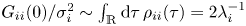 $G_{ii}(0)/\sigma _i^2 \sim \int _\mathbb {R}{{\rm d}}{\tau }\, \rho _{ii}(\tau ) = 2\lambda _i^{-1}$, recalling that
  $\lambda _i^{-1}$ equals the integral time scale (Yaglom Reference Yaglom1962; Tennekes & Lumley Reference Tennekes and Lumley1972). Figure 12 shows that the normalised spectral estimates are close to unity as
  $\omega \to 0$. The normalised model power spectra (3.17) proceed along the same lines to yield
 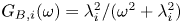 $G_{{B},i}(\omega ) = \lambda _i^2/(\omega ^2 + \lambda _i^2)$. Obviously,
  $G_{{B}_i}(\omega \to 0) \to 1$, as can also be seen in figure 12.
As discussed in § 1, vortex meandering is repeatedly assumed to be associated with some preferred frequency of the order of  $fc/U_\infty \sim 1$. Indeed, if one such meandering frequency exists, then it would show up as a peak in the spectral estimates. On the other hand, it is well known that power spectra computed from finite samples are subject to erratic peaks. The sample power spectra shown in figure 12 display several such potential peaks. Taking a decision on a statistical basis, we consider any peak as significant that has significantly larger variance than the conjectured model power spectrum. Our meandering model assumes a red noise power spectrum (3.17), which is known to admit no preferred frequency. Thus, a suitable statistical test for the existence of any preferred meandering frequency is readily constructed by assuming the null hypothesis that the population has a red noise power spectrum, i.e.
  $H_0: G_{ii}(\omega ) = G_{{B},i}(\omega )$. Assuming (5.21) as the test statistic, a frequency
  $\omega _j$ is significant at the
  $1-\tilde {p}$ level if for the associated squared amplitude estimate
  $\hat {A}_j^2$ we have (Wilks Reference Wilks2006)
 \begin{equation} \hat{A}_j^2 \geq
\frac{G_{B}(\omega_j)}{2K_D}\,\mathfrak{x}_{\tilde{p}}^U,
\quad\text{where}\
\mathfrak{x}_{\tilde{p}}^U: P_{\chi^2(2K_D)}(\mathfrak{x}
\geq \mathfrak{x}_{\tilde{p}}^U) .
\end{equation}
\begin{equation} \hat{A}_j^2 \geq
\frac{G_{B}(\omega_j)}{2K_D}\,\mathfrak{x}_{\tilde{p}}^U,
\quad\text{where}\
\mathfrak{x}_{\tilde{p}}^U: P_{\chi^2(2K_D)}(\mathfrak{x}
\geq \mathfrak{x}_{\tilde{p}}^U) .
\end{equation}The test (5.23) is appropriate for a priori known frequencies, whereas if no such frequency is specified beforehand, then we must account for test multiplicity by the Bonferroni method, yielding the modified test criterion (Wilks Reference Wilks2006)
 \begin{equation} \hat{A}_j^2
\geq
\frac{G_{B}(\omega_j)}{2K_D}\,\mathfrak{x}_{\tilde{p}^*}^U
\quad\text{where}\ \tilde{p}^* = 1
- \alpha^* = 1 - \frac{2\alpha}{N_b} .
\end{equation}
\begin{equation} \hat{A}_j^2
\geq
\frac{G_{B}(\omega_j)}{2K_D}\,\mathfrak{x}_{\tilde{p}^*}^U
\quad\text{where}\ \tilde{p}^* = 1
- \alpha^* = 1 - \frac{2\alpha}{N_b} .
\end{equation}
In (5.24),  $N_{b}/2 = 2048$ is the number of frequencies in the estimator, and
  $\alpha ^* = {5\times 10^{-2}}$ and
  $\alpha \approx 2.4\times 10^{-5}$ are the nominal and actual test levels, respectively. The dashed lines in figure 12 display the squared amplitude threshold resulting from (5.24), beyond which the null hypothesis that there exists no preferred frequency can be rejected at the 5 % level of significance. Since the sample power spectra always remain below this threshold, we conclude that vortex meandering, at least in the present experiment, is not associated with any distinguished characteristic frequency at the given level of significance.
5.7. Ergodicity of vortex meandering
Taking measurements after initial transients have died out, we tacitly assume the dynamics to be characterised by an ergodic probability measure. Thus, taking time averages (as we did throughout) is asymptotically equivalent to computing expectations from the equilibrium ensemble. As is well known, a stochastic process can be ergodic only if it is also stationary (Bendat & Piersol Reference Bendat and Piersol2010), shown to be true in § 5.3. According to Hänggi & Thomas (Reference Hänggi and Thomas1982), finite values of the power spectra as  $\omega \to 0$ further constitute a sufficient condition for ergodicity. This was shown to be the case in figure 12 of § 5.6. As a matter of fact, ergodicity holds for the class of stationary, Gaussian random processes having absolutely continuous power spectra, i.e. having no discrete frequencies associated with distinct periodicities (Bendat & Piersol Reference Bendat and Piersol2010). In §§ 5.3–5.6, we provided statistical evidence that vortex meandering corresponds to a stationary Gauss–Markov process, being a subset of this class. We therefore conclude that vortex meandering in the experiment is ergodic.
6. Conclusion
Meandering constitutes the main manifestation of vortex unsteadiness commonly observed in experiments, and serves as the prototype of the slow vortex response dynamics. In this study, we review previous approaches at explaining the phenomenon, and develop a unified stochastic model in the context of linear response theory. The resulting theory identifies experimental vortex meandering as a form of Brownian motion, and is the first model that is consistent with all fundamental characteristics observed universally in experiments, namely (i) the Gaussian distribution of the vortex position with (ii) growing slow-scale variance downstream and (iii) the broadband power spectral signature.
The statistical identification of characteristic features in experimental data and relating them to theoretical models are ubiquitous problems in physics. However, past fluid dynamics studies regularly resorted to qualitative comparisons and subjective judgements in the interpretation of statistical characteristics. In the present study, we introduce an objective statistical methodology for the systematic and quantitative characterisation of experimental data relative to theoretical models. While this framework is of basic relevance for fluid dynamics experiments in general, we discuss its application to a prototypical problem in experimental vortex dynamics. This allows us to robustly identify experimental vortex meandering with our proposed Brownian-motion-like model at a precisely specified level of certainty.
In particular, working at the 5 % level of significance, we provide statistical evidence that vortex meandering observed in experiments constitutes the manifestation of a stationary Gauss–Markov (Ornstein–Uhlenbeck) process and is therefore ergodic. Physically, this finding is equivalent to stating that vortex meandering is the manifestation of a Brownian motion, as suggested recently by Bölle (Reference Bölle2023). This result implies several important corollaries. Probably most notably, experimental vortex meandering corresponds to a linear dynamics for which, due to Gaussianity, no statistical closure is needed. Due to Gaussianity, the standard deviation (meandering amplitude) constitutes a characteristic perturbation scale. Furthermore, the Markov property identifies vortex meandering with a stochastically memoryless process. Our analysis eventually suggests that the characteristic time scale of the meandering dynamics is not a certain period, as thought previously. Rather, the characteristic meandering time scale  $\lambda _i^{-1}$ is a measure of the vortex response, acting to stabilise, or dampen, external excitation. From a practical perspective, the Markov property and
  $\lambda _i^{-1}$ also indicate a time scale of predictability, which may be relevant for control applications or wake–vortex encounters in aviation.
Acknowledgements
I would like to acknowledge valuable comments from T. Leweke, S. Le Dizès, V. Brion, A. Stephan and three anonymous reviewers, which helped to improve this paper. I am also grateful to ONERA, the French Aerospace Lab, for providing access to the experimental data.
Declaration of interests
The author reports no conflict of interest.
Appendix. Model–experiment comparison in upstream measurement planes
Other than figure 6, this study focuses on a detailed discussion of the experimental vortex meandering characteristics in a single measurement plane at  $z/c = 26$. In this appendix, we show supplementary results from upstream measurement planes at
  $z/c \in \{2,4,12,20\}$ of the same experiment (§ 2.1) that support the proposed Brownian motion meandering model.
Figure 13 shows that the empirical probability densities are well approximated by a Gaussian distribution (as implied by the model) in all measurement planes. They collapse when standardised, i.e. normalised on the standard deviation, as implied by the theory.

Figure 13. Comparison between the standardised normal probability density  $f_{\mathcal {N}}(x_{0,i}\,|\,x_i,t)$ (thick black) with the standardised empirical probability densities
  $\hat {f}(x_{0,i}\,|\,x_i,t)$, assuming 60 bins: (a) first and (b) second principal component time series. Progressively lighter grey colour of the histograms corresponds to more downstream measurement planes (see figure 14 for further details).
Figure 14 shows that the empirical power spectra in the last measurement planes ( $z/c \gtrsim 10$) collapse when scaled on the local variance level and the integral vortex response time scale. The empirical spectra in the first two planes (
 $z/c = 2,4$) qualitatively follow a similar law, but differ quantitatively in the attained variance levels at low frequencies. This difference in the spectral signature seems to be due mainly to the time scale estimates: in the more upstream planes, the dynamics is still close to white noise (flat spectrum). This is consistent with our Brownian-motion-like model. At the same time, it cannot be excluded that other effects not covered by the model contribute to the experimentally observed spectral signature in the first measurement planes. This may be due to the roll-up, transient amplifications, etc. These dynamics are out of the scope of this work.

Figure 14. Comparison between the model power spectrum (3.17) (thick black) with the spectral estimates for the (a) first and (b)second principal component time series.
The spectral trend visible in figure 14 is also consistent with the leading-order vortex response modes. For the given experiment, a dipolar pattern can be identified in the fluctuation vorticity by a POD already in the most upstream measurement plane at  $z/c = 2$ that qualitatively is identical to the one shown in figure 3 (Bölle Reference Bölle2021; Bölle et al. Reference Bölle, Brion, Couliou and Molton2023). The main difference is that, unlike figure 4, this mode contributes only a small fraction to the total variance. Hence, although vortex meandering seems to be present already at the upstream stations (
 $z/c = 2,4$), it has an almost white noise signature. The variance then gradually accumulates in the leading POD modes (Bölle et al. (Reference Bölle, Brion, Couliou and Molton2023) and figure 6). This is the essence of a Brownian motion, and is consistent with the power spectral evolution in figure 14.


 Open access