


1. Introduction
Thermally driven turbulence in liquid metal occurs widely in geophysical and astrophysical systems (Lohse & Shishkina Reference Lohse and Shishkina2023), e.g. in the outer core of the Earth, the convection of liquid iron is believed to be responsible for the generation of Earth's magnetic field (Glatzmaier et al. Reference Glatzmaier, Coe, Hongre and Roberts1999). In these systems, the stabilizing forces produced by rotation or magnetic field are always found to inhibit turbulence (Chandrasekhar Reference Chandrasekhar1961), leading to unexpected enhancement of heat transport (see e.g. Zhong et al. Reference Zhong, Stevens, Clercx, Verzicco, Lohse and Ahlers2009; Lim et al. Reference Lim, Chong, Ding and Xia2019). Recent studies demonstrate that the stabilizing force introduced by spatial confinement in thermal turbulence shows surprisingly similar behaviour as the dynamic constraint by rotation, leading to condensation of the coherent structures and unexpected heat transport enhancement (Huang et al. Reference Huang, Kaczorowski, Ni and Xia2013; Chong et al. Reference Chong, Yang, Huang, Zhong, Stevens, Verzicco, Lohse and Xia2017; Xia et al. Reference Xia, Huang, Xie and Zhang2023). It thus becomes essential to understand how the stabilization effects generated by spatial confinement alter the flow-state evolution, especially the transition to fully developed turbulence in liquid-metal convection.
The classical Rayleigh–Bénard convection (RBC) system is usually employed as a model system to study thermally driven flow. It contains a horizontally infinite fluid layer heated from below and cooled from above (for reviews, see e.g. Ahlers, Grossmann & Lohse Reference Ahlers, Grossmann and Lohse2009; Lohse & Xia Reference Lohse and Xia2010; Chillá & Schumacher Reference Chillá and Schumacher2012; Xia Reference Xia2013). The system is governed by the Oberbeck–Boussinesq equations and the continuity equation below:
 \begin{align} \frac{\partial \boldsymbol{u}}{\partial t}+(\boldsymbol{u}\boldsymbol{\cdot}\boldsymbol{\nabla})\boldsymbol{u}={-}\boldsymbol{\nabla} p+\sqrt{\frac{Pr}{Ra}}\nabla^2 \boldsymbol{u}+T\hat{z}, \quad \frac{\partial T}{\partial t}+(\boldsymbol{u}\boldsymbol{\cdot}\boldsymbol{\nabla}) T=\sqrt{\frac{1}{Ra Pr}}\nabla^2 T,\quad \boldsymbol{\nabla}\boldsymbol{\cdot}\boldsymbol{u} = 0. \end{align}
 The equations (1.1a–c) have been made dimensionless using the cell height  $H$, the temperature difference across the cell
  $\Delta T$, the free-fall velocity
  $u_{ff}=\sqrt {\alpha g \Delta T H}$ and the free-fall time scale
  $\tau _{ff}=H/u_{ff}$. Here
  $\boldsymbol{u}$, p and T are the velocity vector, pressure and temperature, respectively. The vertical unit vector is denoted as
  $\hat{z}$. The RBC system is controlled by two dimensionless parameters, i.e. the Rayleigh number
  $Ra=\alpha g \Delta T H^3/(\nu \kappa )$ and the Prandtl number
  $Pr=\nu /\kappa$. Here
  $\alpha$,
  $\nu$ and
  $\kappa$ are the thermal expansion coefficient, the kinematic viscosity and the thermal diffusivity of the working fluid, respectively. The applied temperature difference and the gravitational acceleration constant are denoted as
  $\Delta T$ and
  $g$, respectively. Studying the regime with strong spatial confinement, characterized by the aspect ratio
  $\varGamma \!=\!D/H<1$ (
 $D$ is the cell diameter) is of particular importance because, from the definition of
  $Ra$, one recognizes that
  $Ra\propto H^3$. It thus becomes relatively easy to achieve high
  $Ra$ with
  $\varGamma <1$ for a cell with fixed
  $D$. However, compared with many studies in the
  $\varGamma \geq 1$ regime (see, for example, Funfschilling et al. Reference Funfschilling, Brown, Nikolaenko and Ahlers2005; Bailon-Cuba, Emran & Schumacher Reference Bailon-Cuba, Emran and Schumacher2010; Van Der Poel, Stevens & Lohse Reference Van Der Poel, Stevens and Lohse2011; Wang et al. Reference Wang, Verzicco, Lohse and Shishkina2020), the effects of the spatial confinement on the flow-state evolution in liquid-metal convection remain obscure.
For the onset of convection, recent theories show that the onset Rayleigh number  $Ra_c\sim \varGamma ^{-4}$ in the limit of
  $\varGamma \ll 1$ (Chandrasekhar Reference Chandrasekhar1961; Shishkina Reference Shishkina2021; Ahlers et al. Reference Ahlers2022; Zhang & Xia Reference Zhang and Xia2023). For a cell with
  $\varGamma =1/10$, similarities between the fluctuations of velocity and temperature statistics are found when compared to a cell with
  $\varGamma =25$ (Pandey et al. Reference Pandey, Krasnov, Schumacher, Samtaney and Sreenivasan2022). In turbulent liquid-metal convection with
  $\varGamma =1/2$, the collapse of the large-scale circulation was reported (Schindler et al. Reference Schindler, Eckert, Zürner, Schumacher and Vogt2022) and a strong coupling between the internal flow structure and heat transport efficiency was found (Chen et al. Reference Chen, Xie, Yang and Ni2023). As
  $Ra$ increases, the liquid-metal convection exhibits rich dynamics, i.e. the flow evolves from conduction to convection, oscillation, chaos and turbulence (Verzicco & Camussi Reference Verzicco and Camussi1997; Ren et al. Reference Ren, Tao, Zhang, Ni, Xia and Xie2022). How the flow-state transitions, especially the onset of convection and the transition to fully developed turbulence, will be altered in the strongly confined regime motivates the present experimental and numerical study.
We will show that with increasing spatial confinement, the flow-state evolution mentioned above remains. The transitional  $Ra$ between different flow states is postponed due to the stabilization effect in the strongly confined cells. However, the transition to the fully developed turbulent state is accelerated in cells with
  $\varGamma \ll 1$ if the flow state is characterized by a supercritical Rayleigh number
  $Ra/Ra_c$. For example, while the flow becomes fully developed turbulence at
  $Ra\approx 200Ra_c$ in a
  $\varGamma =1$ cell, the same transition in a
  $\varGamma =1/20$ cell only requires
  $Ra\approx 3Ra_c$. Using direct numerical simulation (DNS) and linear stability analysis (LSA), we will show that when
  $\varGamma \ll 1$, the system develops multiple vertically aligned rolls just above the onset of convection, allowing more vertical high-wavenumber modes to develop with decreasing
  $\varGamma$. The frequent transitions between different vertical flow modes when
  $Ra$ is increased results in the flow becoming turbulent in a much earlier stage when
  $\varGamma \ll 1$.
2. The experimental and numerical set-ups
The experiment was carried out in cylindrical RBC cells with liquid-metal alloy gallium-indium-tin (GaInSn) as the working fluid. The physical properties of GaInSn are documented in Ren et al. (Reference Ren, Tao, Zhang, Ni, Xia and Xie2022). Its Prandtl number is  $Pr=0.029$ at a mean fluid temperature of
  $35\,^\circ$C. To cover a large
  $Ra$ range, two sets of convection cells with diameters of
  $D=20.14$ mm and
  $D=40.37$ mm were constructed. They are referred to as set A and set B hereafter. For set A, the aspect ratio of the cells vary in the range of
  $1/20\le \varGamma \le 1$. For set B, the aspect ratio changes in the range of
  $1/3\le \varGamma \le 1$. The details on the cell diameter D and height
  $H$ can be found in table 2 in the Appendix. In addition, table 2 lists some parameters of the experiment, such as the range of
  $\Delta T$, applied heat flux at the bottom plate q and the range of Biot number
  $Bi$.
$Bi$.
In total eight convection cells were constructed. They were identical in design. The detailed construction of the convection cell and experimental procedure can be found in Ren et al. (Reference Ren, Tao, Zhang, Ni, Xia and Xie2022). We mention here the essential features of a cell from set A with  $\varGamma =1$. It consists of a top copper cooling plate, a bottom copper heating plate, and a Plexiglas sidewall. The top plate with a diameter of 20.14 mm was cooled by circulating temperature-regulated cooling water. The temperature stability of the cooling water is better than 0.01 K (Julabo, Dyneo DD-1000). The bottom plate was heated with a wire heater embedded in grooves on its backside. The heater was connected to a power supply with a long-term stability of 99.99 % (Ametex, XG 1500). The sidewall with a height of
  $H=20.03$ mm was made of Plexiglas. Its thermal conductivity is 0.192 W (mK)
 $^{-1}$.
Temperatures of the top (bottom) plate were measured using 3 (4) thermistors (Omega, 44031), from which  $Ra$ and
  $Pr$ were calculated. The thermistor heads were located at a distance of 3 mm from the fluid–plate contact surface. The heat flux
  $q$ supplied at the bottom plates was calculated using the measured current
  $I$ and voltage
  $V$ supplied to the heater with a four-wire method, i.e.
  $q=4VI/({\rm \pi} D^2)$. The Nusselt number, which quantifies the ratio between the heat flux transported by the system and that by conduction alone, is calculated using
  $Nu=qH/(\lambda \Delta T)$ with
  $\lambda =24.9$ W (mK)
 $^{-1}$ being the thermal conductivity of GaInSn. The resistances of the thermistors and the voltage supplied to the heater were measured using a digital multimeter (Keysight, 34972A) at a sampling rate of 0.35 Hz. The heat leakage was minimized by adding temperature-controlled side and bottom thermal shields to the cell. The convection cells were levelled better than
  $0.029^\circ$. The temperature boundary condition at the sidewall is approximately adiabatic. The time-averaged spatial temperature homogeneity as measured by 4 (3) embedded thermistors in the bottom (top) plate is within 3 % of
  $\Delta T$. The root-mean-square (r.m.s.) temperatures of the top and bottom plates are within 2 % of
  $\Delta T$ for most of the cells. Two exceptions are the set B cells with
  $\varGamma =1/2$ and 1/3. It is observed that the r.m.s. temperature of the bottom plate in these two cells reaches 6 % and 4 % of
  $\Delta T$. A thermistor with a head diameter of 0.38 mm and a time constant of 30 ms in liquid (Measurement Specialties, GAG22K7MCD419) was placed at the cell centre to probe the temperature fluctuation. In addition, a multi-thermal probe method (Xie, Wei & Xia Reference Xie, Wei and Xia2013) was used to measure the large-scale flow (LSF) structures inside the convection cell. This method could measure the structure and dynamics of LSF in liquid-metal convection accurately (Zürner et al. Reference Zürner, Schindler, Vogt, Eckert and Schumacher2019; Ren et al. Reference Ren, Tao, Zhang, Ni, Xia and Xie2022). Combining the measurements of the temperature fluctuation at the cell centre and the LSF structure and dynamics, the flow states in the five cells with different
  $\varGamma$ can be determined. We refer to Ren et al. (Reference Ren, Tao, Zhang, Ni, Xia and Xie2022) for more details on determining the flow states.
Complementary DNS of the governing Oberbeck–Boussinesq equations was carried out using the CUPS code in the  $1/50\le \varGamma \leq 1$ range. The simulation was conducted in cylindrical domains with no-slip velocity boundary conditions at all walls, adiabatic temperature conditions at the sidewall, and isothermal boundary conditions at the top and bottom plates. For details on the CUPS code and its verification, we refer to Chong, Ding & Xia (Reference Chong, Ding and Xia2018). The
  $Ra_c$ was evaluated from the DNS data. The flow structure at
  $Ra=3Ra_c$ (note
  $Ra_c$ depends on
  $\varGamma$) was simulated to illustrate how spatial confinement alters the flow structures. In addition, LSA was carried out to determine the stability curve of different vertical flow modes.
3. Results and discussions
3.1. The critical Rayleigh number  $Ra_c$ for the onset of convection vs $\varGamma$


In this section, we study how confinement affects the onset of convection. Note that  $Ra_c$ is independent of
  $Pr$ from LSA (Chandrasekhar Reference Chandrasekhar1961). Figure 1(a) plots the measured
  $Nu-1$ as a function of
  $Ra$ together with the scaled time-averaged amplitude
  $\delta /\Delta T$ of the first Fourier mode measured from the azimuthal temperature profile at the midheight of a
  $\varGamma =1$ cell. We have
  $Nu-1=0$ and
  $\delta /\Delta T=0$ in the conduction state. The measured
  $\delta$ aligns with the smallest temperature difference we can resolve experimentally (the dashed line in the figure). However, due to unknown parasitic heat leakage, the
  $Nu$ measured in the conduction state is slightly above 1. Combining
  $Nu$ and
  $\delta$ measurements, we conclude that the system starts from the conduction state at
  $Ra\sim 4000$ and evolves into the convection state with increasing
  $Ra$. The inset shows the streamlines of the flow field obtained at
  $Ra\approx Ra_c$ numerically in a
  $\varGamma=1$ cell with red and blue colours representing ascending and descending flow, respectively. The LSF is a single-roll structure, consistent with the observation that the first Fourier mode is the dominant mode obtained from the sidewall temperature profiles.

Figure 1. (a) Determination of the critical Rayleigh number  $Ra_c$ for the onset of convection in a
  $\varGamma =1$ cell based on
  $Nu$ (squares) and the amplitude
  $\delta /\Delta T$ of the LSF (circles) obtained from experiment. (b) The
  $Ra_c$ vs
  $\varGamma$ from present experiment and DNS. The dashed line marks
  $Ra_c\sim \varGamma ^{-4.05}$ fitted to the data with
  $\varGamma \le 1/10$. The solid line is a theoretical prediction from Shishkina (Reference Shishkina2021). The triangles are
  $Ra_c$ measured in the
  $\varGamma \ge 1$ regime with
  $Pr=28.9$ from Hébert et al. (Reference Hébert, Hufschmid, Scheel and Ahlers2010).
It was predicted theoretically that the  $Nu$ just above the onset of convection depends linearly on
  $Ra$ (Malkus & Veronis Reference Malkus and Veronis1958). Thus, by fitting the
  $Nu$ data deviated from the horizontal dashed line (the conduction state) and finding the intersection point between the extrapolation of this linear fitting function with the horizontal dashed line, we determine
  $Ra_c=5170$ from
  $Nu$ measurement. Figure 1(a) also shows that
  $\delta /\Delta T$ increases linearly with
  $Ra$ just above onset. Similar to
  $Nu-1$, we can also determine
  $Ra_c$ from
  $\delta /\Delta T$ by the linear fitting method, which yields
  $Ra_c=5095$. The two values of
  $Ra_c$ agree with each other within 2 %.
The above analysis of  $Nu$ measured experimentally in the range of
  $1/20\le \varGamma \le 1/2$ and that obtained numerically for
  $1/50\le \varGamma \le 1$ were repeated. The so-determined
  $Ra_c$ as a function of
  $\varGamma$ is plotted in figure 1(b). The experimentally determined
  $Ra_c$ agrees with the numerically obtained
  $Ra_c$. Similar to the observation by Zhang & Xia (Reference Zhang and Xia2023) and Müller, Neumann & Weber (Reference Müller, Neumann and Weber1984), with decreasing
  $\varGamma$,
  $Ra_c$ shows a rapid increase. For comparison, we also plot in the figure
  $Ra_c$ measured experimentally for
  $\varGamma \ge 1$ in a working fluid with
  $Pr=28.9$ from Hébert et al. (Reference Hébert, Hufschmid, Scheel and Ahlers2010) and the theoretical prediction of
  $Ra_{c,\varGamma }=(2{\rm \pi} )^4(1+(1.4876/\varGamma ^2))(1+(0.3435/\varGamma ^2))$ from Shishkina (Reference Shishkina2021) with adiabatic sidewall temperature boundary conditions. Figure 1(b) shows the experimental data, numerical data and theoretical prediction agree excellently with each other over almost three decades in
  $\varGamma$. The results also imply the sidewall boundary condition of the experiment can be treated as adiabatic to a good approximation. In addition, when
  $\varGamma \le 1/10$, the data can be fitted by
  $Ra_c=915\varGamma ^{-4.05}$ (the dashed line).
3.2. Flow-state evolution in spatially confined cells ($\varGamma <1$)

We now study the flow-state evolutions when  $Ra$ increases beyond
  $Ra_c$. Previous studies in liquid-metal convection with
  $\varGamma =1$ show that the flow evolves from the convection state to an oscillation state, a chaotic state, a transition-to-turbulence state and a fully developed turbulent state (Verzicco & Camussi Reference Verzicco and Camussi1997; Ren et al. Reference Ren, Tao, Zhang, Ni, Xia and Xie2022). The different flow states exhibit different natures of the temperature fluctuations at the cell centre. For the convection state, there is hardly any temperature fluctuation. The scaled r.m.s. temperature at the cell centre
  $\sigma _{T_c}/\Delta T$ increases beyond zero when the system becomes time-dependent, i.e. in the oscillation state. In the chaotic state and the transition-to-turbulence state,
  $\sigma _{T_c}/\Delta T$ increases with
  $Ra$. But these two states are characterized by different scaling relations between
  $\sigma _{T_c}/\Delta T$ and
  $Ra$. The
  $\sigma _{T_c}/\Delta T$ reaches maximum at the boundary between the transition-to-turbulence state and the fully developed turbulence state. When the system becomes fully developed, one observes a negative scaling law between
  $\sigma _{T_c}/\Delta T$ and
  $Ra$ that is widely observed in working fluid like water (see, for example, Xie et al. Reference Xie, Cheng, Hu and Xia2019). Thus, the transitional value of
  $Ra$ between different states can be determined based on the temperature fluctuation measured at the cell centre.
Figures 2(a)–2(d) plot the scaled temperature fluctuation in cells with  $\varGamma =1/2$, 1/3, 1/10 and 1/20, respectively. Following Ren et al. (Reference Ren, Tao, Zhang, Ni, Xia and Xie2022), the temperature fluctuations for different states are fitted by respective power laws. The transitional Rayleigh numbers between different states are then determined when two power laws cross. The so-determined flow states are labelled in figure 2. Note the flow-state transition can also be determined from the dynamics of the LSF, i.e. its flow strength
  $\delta$, azimuthal orientation
  $\theta$, and their respective fluctuations. The boundaries between different flow states show no noticeable qualitative difference based on either the temperature fluctuation method or the dynamics of the LSF.

Figure 2. Determination of the flow state based on the experimentally measured scaled temperature fluctuations at the cell centre  $\sigma _{T_c}/\Delta T$ as a function of
  $Ra$ in cells with (a)
  $\varGamma =1/2$; (b)
  $\varGamma =1/3$; (c)
  $\varGamma =1/10$ and (d)
  $\varGamma =1/20$. The blue squares represent data measured in the set A cells and the red circles in (a,b) are data measured in the set B cells. In (b) the SR and DR refer to single-roll and double-roll, respectively.
To study systematically the effects of  $\varGamma$ on flow-state evolution, we plot the flow state in a two-dimensional phase space composed of either
  $\varGamma -Ra$ or
  $\varGamma -(Ra/Ra_c)$. The results are plotted in figures 3(a) and 3(b), respectively. Note in figure 3(b),
  $Ra$ for each
  $\varGamma$ is normalized by its own
  $Ra_c$. We first examine the flow-state evolution in the
  $\varGamma -Ra$ plot. One sees that the flow in cells with
  $1/20\le \varGamma \le 1$ all exhibit a conduction state, a convection state, an oscillation state, a chaotic state, a transition-to-turbulence state and a fully developed turbulent state. However, with decreasing
  $\varGamma$, significant changes in the flow-state transition can be observed. Not only
  $Ra_c$ is postponed to larger values as discussed in § 3.1. The transitional values of the other flow states are all postponed to larger
  $Ra$ due to the stabilization effect caused by spatial confinement. The transitional Rayleigh number to the fully developed turbulent state, defined as
  $Ra_f$ here (see purple left-pointing triangles in figure 3a) can be fitted by a power law with
  $\varGamma$ for
  $\varGamma \le 1/3$, i.e.
  $Ra_f=5.40\times 10^4\varGamma ^{-3.01}$. The results suggest that the damping effect on the transition to the fully developed turbulent state by the stabilization effects of the wall when decreasing
  $\varGamma$ becomes weak when compared with that on the onset of convection, which is
  $Ra_c\sim \varGamma ^{-4.05}$. It should be noted that the
  $Ra_f\sim \varGamma ^{-3.01}$ scaling is only valid in the studied parameter range, i.e,
  $1/20\le \varGamma \le 1/3$. In addition, we note if the observed scaling is valid for
  $\varGamma \ll 1$, one obtains
  $Ra_f/Ra_c\sim \varGamma ^{-3.01}/\varGamma ^{-4.05}\sim \varGamma$. However, since the
  $\varGamma$ is not asymptotically small and the range of
  $\varGamma$ in the present study is limited, one sees that
  $Ra_f/Ra_c\sim \varGamma ^{1.33}$ to the first order as shown in figure 3(b). It will be very interesting to study what will happen when
  $\varGamma$ becomes even smaller than the present study.

Figure 3. (a) Experimentally obtained flow-state evolution in the  $\varGamma -Ra$ phase space. The flow states are marked by different colours indicated in the legend. The symbols are experimentally determined transitional Rayleigh numbers between different flow states. The solid lines are used to guide the eye. The lower dashed line marks the onset Rayleigh number
  $Ra_c=915\varGamma ^{-4.05}$ and the upper dashed line marks the transition to fully developed turbulence Rayleigh number
  $Ra_f=5.40\times 10^4\varGamma ^{-3.01}$. (b) The phase diagram plotted in the
  $\varGamma -(Ra/Ra_c)$ phase space. The dashed line is a fitting of
  $Ra_f/Ra_c\sim \varGamma ^{1.33}$.
Although we do not have a theoretical understanding of this  $\varGamma ^{-3.01}$ dependence, we note a similar
  $\varGamma ^{-3}$ dependence for the transition to the ultimate state in turbulent RBC with gas as the working fluid was reported (Roche et al. Reference Roche, Gauthier, Kaiser and Salort2010; Ahlers et al. Reference Ahlers2022; He, Bodenschatz & Ahlers Reference He, Bodenschatz and Ahlers2022). As we will show later, the transition to the fully developed turbulent state is characterized by the loss of spatial coherence of the LSF. In contrast, the transition to the ultimate regime results from the boundary layer becoming turbulent (Kraichnan Reference Kraichnan1962). Thus, the two
  $\varGamma ^{-3}$ scalings may originate from different flow physics.
Now let us discuss the flow-state evolution in the  $\varGamma -(Ra/Ra_c)$ plot shown in figure 3(b), which is usually employed when studying flow-state transitions in the vicinity of onset. When
  $\varGamma$ is changed from 1 to 1/2, one sees that all the transitions are advanced, occurring at smaller values of
  $Ra/Ra_c$. The initiation of the oscillation instability occurs at
  $Ra/Ra_c\approx 1.6$, and it is almost independent of
  $\varGamma$ for
  $1/20 \le \varGamma \le 1/3$. For
  $1/20\le \varGamma \le 1/10$, the transition from the oscillation state to the chaotic state and that from the chaotic state to the transition-to-turbulence state occur at
  $Ra/Ra_c=1.68$ and
  $Ra/Ra_c=1.86$, respectively. Both seem to be independent of
  $\varGamma$. The enlarged portion of the oscillation state and the consequent delay of the chaotic state in the cell with
  $\varGamma =1/3$ originates from a bifurcation of the flow from a single-roll (SR) structure to a double-roll (DR) structure, which we will discuss in detail elsewhere (authors' unpublished observations). Figure 3(b) also reveals that the transition to fully developed turbulence occurs at a much earlier stage for smaller
  $\varGamma$, e.g. the flow in the
  $\varGamma =1$ cell becomes fully developed turbulence at
  $Ra\approx 200Ra_c$. It occurs at
  $Ra\approx 3Ra_c$ in the cell with
  $\varGamma =1/20$. The observation suggests that despite delaying the onset of convection due to the stabilization effects caused by strong spatial confinement, it advanced the transition to turbulence. Thus, slender geometries could be utilized to achieve fully developed turbulence in a relatively accessible way by reducing the cell diameter.
Recently, Zhang & Xia (Reference Zhang and Xia2023) studied heat transport in slender cuboid RBC using water as the working fluid with the  $Pr=4.38$. They classified the flow states in their quasi-one-dimensional cells based on the heat transport behaviour of the system, i.e. a viscous-dominated regime, a plume-controlled regime and a classical boundary-layer-controlled regime. The present study differs from Zhang & Xia (Reference Zhang and Xia2023) in two ways: firstly, we are working with
  $Pr$ which is two orders of magnitude smaller than that reported in Zhang & Xia (Reference Zhang and Xia2023); secondly, the phase diagram shown in figure 3 is not based on the heat transport, but based on the structure and dynamics of the flow.
3.3. Dynamics of the LSF with decreasing $\varGamma$

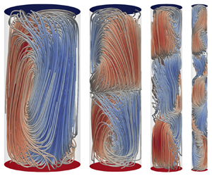
To reveal the mechanism that accelerates the transition to turbulence in strongly confined cells, we study the structure and dynamics of the LSF. Figures 4(a)–4(f) show the instantaneous flow structure numerically obtained at  $Ra/Ra_c=3$ in cells with
  $1/20 \le\varGamma\le1$. Supplementary movies are available at https://doi.org/10.1017/jfm.2024.86 showing the temporal evolution of the flow structure. While the flow is in the convection state for
  $\varGamma =1$, the oscillation state for
  $\varGamma =1/2$ and 1/3, the chaotic state for
  $\varGamma =1/5$, it is in the turbulent state for
  $\varGamma \le 1/10$. Following Zwirner, Tilgner & Shishkina (Reference Zwirner, Tilgner and Shishkina2020), we use the relation between the horizontally averaged squared horizontal velocity
  $E_h=\sum _{i=x,y}\langle u_{i}^2\rangle _S/U_S^2$ and the squared vertical velocity
  $E_v=\langle u_{z}^2\rangle _S/U_S^2$ to identify the flow structures. Here
  $\langle \cdots \rangle _S$ means averaging over a horizontal cross-section and
  $U_S^2=\sum _{i=x,y,z}\langle u_{i}^2\rangle _S$ is the total energy at a certain horizontal cross-section. The left subplot of each panel in figure 4 shows the streamlines with red and blue colours representing ascending and descending flow, respectively. The right subplot of each panel shows the vertical profiles of
  $E_h$ (blue line) and
  $E_v$ (red line). For a continuous vertical roll to exist, we require
  $E_v(z)>E_h(z)$. To determine the junction between two neighbouring rolls, we first find two neighbouring
  $E_v(z)=E_h(z)$ points. The midpoint of these two neighbouring points with
  $E_h(z)>E_v(z)$ is then defined as the junction between two rolls (see the dashed line in the right subplots of each panel in figure 4). From figure 4(a,b), one sees that for
  $\varGamma =1$ and 1/2, the LSF is in the form of a single-roll structure similar to the onset of convection (inset of figure 1a). This is also verified by the observation that
  $E_v>E_h$ for the entire cell except for the locations very close to the top and bottom boundaries where large parts of the flow in the boundary layers are in the horizontal directions, resulting in
  $E_h>E_v$. When
  $\varGamma \le 1/3$, the flow structure becomes complex: a double-roll structure in the
  $\varGamma =1/3$ cell and a triple-roll structure in the
  $\varGamma =1/5$ cell. There are eight vertically stacked rolls for the extreme case with
  $\varGamma =1/20$.

Figure 4. Numerically obtained instantaneous flow structure at  $Ra/Ra_c=3$ for (a)
  $\varGamma =1$ with number of rolls being
  $n=1$ ; (b)
  $\varGamma =1/2$,
  $n=1$; (c)
  $\varGamma =1/3$,
  $n=2$; (d)
  $\varGamma =1/5$,
  $n=3$; (e)
  $\varGamma =1/10$,
  $n=6$; and (f)
  $\varGamma =1/20$,
  $n=8$. For each panel, the left subplot shows the streamlines with red and blue colours representing ascending and descending flow, respectively. The right subplot shows the vertical profiles of the horizontally averaged normalized squared horizontal velocity
  $E_h(z)=\sum _{i=x,y}\langle u_{i}^2(z)\rangle _S/U_S^2(z)$ (blue line) and the squared vertical velocity
  $E_v(z)=\langle u_z^2(z)\rangle _S/U_S^2(z)$ (red line). Here
  $\langle \cdots \rangle _S$ means averaging over a horizontal cross-section and
  $U_S^2(z)=\sum _{i=x,y,z}\langle u^2_{i}(z)\rangle _S$ is the total energy at a certain
  $z$. The horizontal dashed lines mark the boundary between adjacent rolls.
To study systematically the temporal evolution of the flow structure, we show in figure 5 the time trace of the number of rolls  $n$, the corresponding
  $Nu$ and
  $Re$. Table 1 summarizes the statistics of different flow modes in cells with
  $1/20\le \varGamma \le 1/2$, including their mean lifetime
  $\tau$, the probability of occurrence
  $P$ and the corresponding
  $Nu$. The symbol ‘—’ means no such flow mode is observed during the simulation, which runs at least 1800
  $\tau _{ff}$. In the
  $\varGamma =1$ cell (not shown), the structure of the LSF is a stable single roll similar to the instantaneous examples shown in figure 4(a). When decreasing
  $\varGamma$, one sees that, firstly, the maximum number of rolls the system can develop
  $n_{max}$ increases significantly from
  $n_{max}=1$ for
  $\varGamma =1$ to
  $n_{max}=11$ for
  $\varGamma =1/20$. Secondly, the system switches more frequently between flow mode with different
  $n$ for smaller
  $\varGamma$, e.g. for the
  $\varGamma =1/3$ cell, the system switches almost periodically between the
  $n=1$ and
  $n=2$ modes; it switches frequently and chaotically between flow modes from
  $n=1$ to
  $n=13$ in the
  $\varGamma =1/20$ cell. As a result of the increased number of rolls and frequent switching among them, the average lifetime of each mode decreases dramatically with decreasing
  $\varGamma$. For example, in the
  $\varGamma =1/3$ cell, the mean lifetime
  $\tau$ for the
  $n=1$ and the
  $n=2$ modes are
  $\tau _{1}=14.61\tau _{ff}$ and
  $\tau _{2}=5.21\tau _{ff}$, respectively. In contrast, in the
  $\varGamma =1/20$ cell, due to the frequent transitions between modes with different
  $n$, the mean lifetime of each mode is less than
  $\tau _{ff}$. The maximum lifetime observed is
  $\tau _{1}=0.75\tau _{ff}$ and the minimum mean lifetime observed is
  $\tau _{10}=0.18\tau _{ff}$. These observations suggest that in the strongly confined cells, the single-roll large-scale circulation observed in systems with
  $\varGamma \sim 1$ collapses. As a result of this new dynamical process of flow-mode transition discussed above that exists only in confined geometries, the flow becomes turbulent very quickly after the onset of convection.

Figure 5. Time series of the number of rolls  $n$ (blue solid line), the Nusselt number
  $Nu$ (black dashed line) and the Reynolds number
  $Re$ (red dash-dotted line) in cells with (a)
  $\varGamma =1/3$; (b)
  $\varGamma =1/5$; (c)
  $\varGamma =1/10$; and (d)
  $\varGamma =1/20$ obtained numerically at
  $Ra/Ra_c=3$. In the vertical axis title, X represents either Nu, Re or n, and
  $\sigma_X$ represents their respective r.m.s. value.
Table 1. The mean lifetime  $\tau$ in units of free-fall time
  $\tau _{ff}$, the probabilities of occurrence
  $P$ and the mean heat transport efficiency
  $Nu$ of the
  $n$-roll flow mode for
  $Ra/Ra_c=3$ at
  $Pr=0.029$. The symbol ‘—’ means no such flow modes are observed in the study. Each simulation runs at least 1800
  $\tau _{ff}$ after the system has reached a steady state.

The change in the flow state with  $\varGamma$ is also reflected on the
  $Nu$ and
  $Re$ time series shown in figure 5. One sees that both
  $Nu$ and
  $Re$ oscillate periodically in the cell with
  $\varGamma =1/3$. With decreasing
  $\varGamma$, the fluctuation of
  $Nu$ and
  $Re$ increases. They reach up to four times the r.m.s. value in the
  $\varGamma =1/20$ cell. Consistent with the finding by Zwirner et al. (Reference Zwirner, Tilgner and Shishkina2020), for a given
  $\varGamma$, the higher the number of vertical rolls, the smaller the heat transport efficiency of the system. For example, in the cell with
  $\varGamma =1/20$, the maximum
  $Nu$ observed for
  $n=1$ mode is 50 % higher than
  $Nu$ of the
  $n=11$ mode. It should also be noted that there is a negative time delay between
  $n$ and
  $Nu$ or
  $Re$, suggesting that the flow-mode change is probably the cause for the variation in
  $Nu$ and
  $Re$.
$Re$.
Finally, let us try to understand the origin of the multiple vertically stacked rolls based on LSA. We consider an RBC cell with no-slip and constant temperature boundary conditions at the top and bottom walls. The two horizontal directions are periodic. The height of the cell  $H$ is fixed to be 1. Thus, its aspect ratio is
  $\varGamma =D/H=D$. Limiting the discussion with only one cell in the horizontal direction requires
  $k_xD={\rm \pi}$. Following the standard LSA procedure (Chandrasekhar Reference Chandrasekhar1961), we obtain the marginal stability curve for the cell with the horizontal wavenumber
  $k^2=k_x^2+k_y^2=2k_x^2$ and different numbers of vertically stacked rolls
  $n$. Here
  $k_x$ and
  $k_y$ are the two horizontal wavenumbers. Next we replace
  $k$ from the LSA analysis with
  $\varGamma$ using the relation
  $\varGamma ={\rm \pi} /k_x={\rm \pi} /k_y=\sqrt {2}{\rm \pi} /k$. Figure 6(a) plots the marginal stability curve from
  $n=1$ to
  $n=10$ vertically stacked rolls in the
  $Ra-\varGamma$ diagram. Firstly, it is seen that the marginal stability curves for different modes do not cross each other with decreasing
  $\varGamma$. Secondly, the curves for the
  $n>1$ modes gradually approach the limit of
  $Ra_{c,n=1}=390\varGamma ^{-4}$ (the dashed line) for
  $\varGamma \ll 1$, suggesting that in the strongly confined regime, the high-order modes become unstable just above the onset of convection. This can be seen more clearly from figure 6(b), where the marginal stability curves for the
  $n>1$ modes are normalized by that of the
  $n=1$ mode. The figure suggests that for
  $Ra=3Ra_c$ and
  $\varGamma <1/10$, all modes up to
  $n=9$ will grow, consistent with the DNS observation.

Figure 6. (a) Marginal stability curve for different numbers of vertically aligned rolls  $n$ vs the aspect ratio
  $\varGamma$. The dashed line marks
  $Ra_c\sim \varGamma ^{-4}$ for the
  $n=1$ mode. (b) The marginal stability curve of the
  $n>1$ modes normalized by that of the
  $n=1$ mode as a function of
  $\varGamma$.
4. Conclusion
We have systematically studied the flow-state evolution in liquid-metal convection in a strongly confined regime. Combining experiment, DNS and LSA, we show that not only the onset of Rayleigh–Bénard instability is delayed due to the stabilizing effect in strongly confined geometries, but the various flow-state transitions are all postponed. The onset Rayleigh number  $Ra_c$ and the transition to fully developed turbulence Rayleigh number
  $Ra_f$ depend on the aspect ratio
  $\varGamma$ with
  $Ra_c\sim \varGamma ^{-4.05}$ for
  $\varGamma \le 1/10$ and
  $Ra_f\sim \varGamma ^{-3.01}$ for
  $\varGamma \le 1/3$, implying that the stabilization effects are weaker on the transition to fully developed turbulence when compared with that on the onset. The study shows that spatial confinement facilitates the transition to turbulence if the flow-state transition is expressed in terms of a supercritical Rayleigh number, i.e.
  $Ra/Ra_c$. The reason for this can be attributed to a new mechanism for transition to turbulence in the strongly confined limit. The LSA shows high-order vertical flow modes appear just above the onset of convection in strong spatially confined cells. With increasing
  $Ra$, the system stochastically switches between different vertical flow modes. As a result of this frequent flow-mode switching, the usually observed single-roll structure in the
  $\varGamma \sim 1$ regime breaks down, and the system becomes fully developed turbulence in an early stage. Turbulence with stabilization forces is common in nature and industry, such as rotation and magnetic fields in geophysical and astrophysical applications. The newly discovered mechanism for transition to fully developed turbulence may find applications in other turbulent flows.
Supplementary movies
Supplementary movies showing the temporal evolution of the large-scale flow structure in different  $\varGamma$ cells are available at https://doi.org/10.1017/jfm.2024.86.
Acknowledgements
We are grateful to R. Kerswell for pointing us to the analysis of the problem using LSA. We also thank C. Sun, S.-D. Huang and L. Zhang for discussions.
Funding
This work was supported by the NSFC grant nos 92152104, 12232010, 12072144 and a XJTU Young Talent Support Plan.
Declaration of interests
The authors report no conflict of interest.
Author contributions
L.R. and X.T. contributed equally to this work.
Appendix
Table 2 lists some of the parameters of the convection cells and of the experiment in the present study. In total, eight convection cells were used. In the table, the cell diameter  $D$, height
  $H$, the aspect ratio
  $\varGamma$, the range of temperature difference between the top and bottom plate
  $\Delta T$, the range of the heat flux q supplied at the bottom plate and the Biot number
  $Bi$ are listed.
Table 2. Some parameters of the convection cells and of the experiment. Here  $\varGamma =D/H$ is the aspect ratio of the cell with
  $D$ and
  $H$ being the cell diameter and height, respectively. The nominal
  $\varGamma$ is used to refer to each cell in the main text;
  $\Delta T=T_{bot}-T_{top}$ denotes the time-averaged temperature difference between the bottom plate
  $T_{bot}$ and the top plate
  $T_{top}$. The heat flux supplied at the bottom plate is listed as
  $q$. The range of the Biot number, defined as
  $Bi=Nu(\lambda /\lambda _{Cu})(H_{Cu}/H))$, is shown in the last column for each cell with
  $\lambda _{Cu}=401$ W (mK)
 $^{-1}$ and
  $H_{Cu}=19$ mm for the bottom plate and 15 mm for the top plate.


