


1. Introduction
The high-frequency sampling of flow data has increasingly drawn attention in the turbulence research community as it has become an important means for understanding the underlying fluid dynamics within the turbulence kinetic energy cascade. However, there remains a great challenge in developing hardware for acquiring highly time-resolved turbulence data, compromising the balancing of the spatial resolution and temporal sampling rate. Although data-driven reconstruction techniques, such as linear stochastic estimation (LSE) and machine learning (ML), have brought new impetus to super-temporal-resolution (STR) reconstruction using time-sparse spatially resolved flow fields, the resultant evolution at small scales is commonly incorrect owing to the reduced-order reconstruction, the lack of physical constraint or insufficient temporal information in the training database. This leads to high demand for the development of model-assisted data-driven techniques such as data assimilation (DA).
As one of the earliest approaches for STR reconstruction, LSE (Adrian & Moin Reference Adrian and Moin1988) attempts to integrate the advantages of a high spatial resolution in field-based measurements and a high sampling rate of probe signals. It has been established on the foundation of non-local flow properties and was widely used in early studies for time-resolved reduced-order reconstruction. Relatively inexpensive discrete probes provide high-sampling-rate measurement data while capturing not only the temporal information but also some degree of the spatial information in flow fields. Linear stochastic estimation approximates the conditional averages of the fields in terms of the measurement data and has been sequentially modified to couple with proper orthogonal decomposition (POD) in the estimation of the time series of mode amplitudes used to reconstruct reduced-order flow fields (Hudy, Naguib & Humphreys Reference Hudy, Naguib and Humphreys2007; Tinney, Ukeiley & Glauser Reference Tinney, Ukeiley and Glauser2008). However, the implementation of LSE is mainly suited to the reduced-order reconstruction of flows having periodic or quasi-periodic behaviours, and the resultant realisations are built in preference to energetic large-scale flow structures represented by several leading POD modes. Moreover, LSE suffers from the problem of overfitting through the amplification of singular eigenvalues of small amplitude (Podvin et al. Reference Podvin, Nguimatsia, Foucaut, Cuvier and Fraigneau2018). Although such a process has been improved using the multi-time-delay approach (Durgesh & Naughton Reference Durgesh and Naughton2010; Kerherve, Roux & Mathis Reference Kerherve, Roux and Mathis2017), the Kalman smoother (Tu et al. Reference Tu, Griffin, Hart, Rowley, Cattafesta and Ukeiley2013), a new variant of the formulation (Podvin et al. Reference Podvin, Nguimatsia, Foucaut, Cuvier and Fraigneau2018) and multichannel singular spectrum analysis (Hosseini, Martinuzzi & Noack Reference Hosseini, Martinuzzi and Noack2015), there remains a connatural limitation when there are far fewer probes than degrees of freedom of the flow fields. This limits the number of POD modes that can be used in the LSE reconstruction and induces error in amplitude determination. The limitation becomes important when the flow is broad-band and little kinetic energy is contained in the leading POD modes.
Due to the rapid development of computer science in recent years, ML techniques have been widely used in fluid dynamic research including flow and heat transfer prediction (Lee & You Reference Lee and You2019; Kim & Lee Reference Kim and Lee2020), turbulence modelling (Duraisamy, Iaccarino & Xiao Reference Duraisamy, Iaccarino and Xiao2019; Sirignano & MacArt Reference Sirignano and Macart2023) and active control (Park & Choi Reference Park and Choi2020; Pino et al. Reference Pino, Schena, Rabault and Mendez2023). Comprehensive reviews on ML-augmented fluid mechanics were presented by Brenner, Eldredge & Freund (Reference Brenner, Eldredge and Freund2019) and Brunton, Noack & Koumoutsakos (Reference Brunton, Noack and Koumoutsakos2019). As a representative application using ML techniques, super-resolution reconstruction can be achieved by constructing a convolutional neural network that directly maps the low-resolution fields to the high-resolution fields once trained using both a low- and a high-resolution database (Fukami, Fukagata & Taira Reference Fukami, Fukagata and Taira2019; Liu et al. Reference Liu, Tang, Huang and Lu2020). In addition, high-sampling-rate training data can be used for STR reconstruction (Fukami, Fukagata & Taira Reference Fukami, Fukagata and Taira2021). While these supervised deep-learning models require labelled low- and high-resolution data pairs for training, unpaired data are more practical to use as noted by Kim et al. (Reference Kim, Kim, Won and Lee2021), who proposed an unsupervised deep-learning model for super-resolution reconstruction adopting a cyclic-consistent generative adversarial network. However, purely ML methods often yield non-physical features when the resolution ratio between the target and input fields is large due to the lack of physical constraint in the data-driven optimisation process. The approach based on POD or extended POD, similar to that used in LSE, is usually adopted to avoid irregular prediction. It has been demonstrated that ML techniques account for nonlinearities in flows in the interpolation of the model coefficients and thus perform better in reconstructions using more POD modes than the conventional LSE approach. Recent work has demonstrated the advantages of ML approaches over LSE in reduced-order STR reconstruction (Deng et al. Reference Deng, Chen, Liu and Kim2019; Guemes, Discetti & Ianiro Reference Guemes, Discetti and Ianiro2019; Giannopoulos & Aider Reference Giannopoulos and Aider2020; Jin et al. Reference Jin, Laima, Chen and Li2020). Although POD-based approaches enable us to recover the main dynamic patterns of the turbulence fluctuations in STR reconstruction, the high-order modes with temporally varying frequencies higher than the sampling rate pose a challenge. The aforementioned works largely aimed at understanding either large-scale motion in the flows or flow feedback control. Additionally, the approaches are only applicable to statistically stable flows as a large database is required in the training process. In the fields of computer vision and video processing, STR reconstruction is commonly known as frame interpolation (Niklaus, Mai & Liu Reference Niklaus, Mai and Liu2017; Chi et al. Reference Chi, Nasiri, Liu, Lu and Plataniotis2020; Bao et al. Reference Bao, Lai, Zhang, Gao and Yang2021) and is widely used to artificially increase the frame rate of a video by creating fake frames containing sufficient image details between real frames. However, similar studies have rarely been conducted for turbulent flows with the recovery of small-scale structures having evolution frequencies much higher than the sampling rate.
Being different from the purely data-driven techniques, DA (Evensen, Vossepoel & Leeuwen Reference Evensen, Vossepoel and Leeuwen2022) integrates measurement data (observations) with physical or semi-physical equations (predictive models). Thus, DA avoids irregular motions of the reproduced vortical structures and substantially reduces the training database requirement, and it is undoubtedly an important approach to increasing the data reach and augmenting methodology interpretability. Data assimilation has been applied in fluid mechanics for acoustic state and model parameter predictions using the Bayesian ensemble method (Nóvoa & Magri Reference Nóvoa and Magri2022), ocean wave forecasting using the high-order spectral method coupled with the ensemble Kalman filter (Wang & Pan Reference Wang and Pan2021) and data-driven numerical simulation using a nudging strategy (Zauner et al. Reference Zauner, Mons, Marquet and Leclaire2022). Among various DA algorithms, variational DA benefits from the driving of adjoint equations and is able to determine the optimal field with extremely large dimensions and a lower data requirement. Variational DA includes the three-dimensional type for steady-state processes (Foures et al. Reference Foures, Dovetta, Sipp and Schmid2014; Mons & Marquet Reference Mons and Marquet2021) and four-dimensional type (4D-Var) for unsteady-state prediction (Chandramouli, Memin & Heitz Reference Chandramouli, Memin and Heitz2020). In addition, variational DA can be implemented in either discrete or continuous form. The former implementation discretises the system before the derivation of the adjoint equation, which has a large memory requirement for expensive matrix computation (Papoutsis-Kiachagias & Giannakoglou Reference Papoutsis-Kiachagias and Giannakoglou2016), and the latter implementation is thus preferred for complex flow configurations (Foures et al. Reference Foures, Dovetta, Sipp and Schmid2014; He et al. Reference He, Liu and Gan2018a; Li et al. Reference Li, Zhang, Dong and Abdullah2019; Chandramouli et al. Reference Chandramouli, Memin and Heitz2020; He, Wang & Liu Reference He, Wang and Liu2021). We focus on 4D-Var as the unsteady state is the current topic of interest. Four-dimensional variation is a generalisation of three-dimensional variation that handles observations distributed in time. It thus optimises the constraint problem via an objective function presenting the deviation of the model forecast from the observations in time integration. The classical strong-constraint 4D-Var (Evensen et al. Reference Evensen, Vossepoel and Leeuwen2022; Wang, Wang & Zaki Reference Wang, Wang and Zaki2022) seeks an initial condition such that the forecast best fits the observations within the assimilation interval, under the assumption that a precise predictive model entirely determines the true state once initialised. Its applications in fluid mechanics include the determination of the inflow and initial conditions for direct numerical simulation (Gronskis, Heitz & Mémin Reference Gronskis, Heitz and Mémin2013), the de-noising of particle image velocimetry (PIV) data (Gillissen, Bouffanais & Yue Reference Gillissen, Bouffanais and Yue2019) and the reconstruction of small-scale structures in Kolmogorov flows (Li et al. Reference Li, Zhang, Dong and Abdullah2019). However, in the case of turbulent flows, 4D-Var is prone to be a weak constraint (Bennett Reference Bennett2002; Tremolet Reference Tremolet2007) owing to the error in the predictive models induced by either the subgrid stress or the inappropriate boundary conditions. Weak-constraint 4D-Var has not yet been extensively considered for turbulent flows, except in a few studies involving the simple example of the reactive–diffusive equation (Vidard et al. Reference Vidard, Blayo, Dimet and Piacentini2000), the development of POD-based reduced-order models in turbulence dynamics (Artana et al. Reference Artana, Cammilleri, Carlier and Mémin2012; Stefanescu, Sandu & Navon Reference Stefanescu, Sandu and Navon2015) and stochastic model-error assimilation in a turbulent wake (Chandramouli et al. Reference Chandramouli, Memin and Heitz2020). In addition, STR reconstruction using weak-constraint 4D-Var is suited to turbulence research, yet this has not been considered in previous work.
This paper concentrates on STR reconstruction beyond the Nyquist limit with the recovery of vortex temporal evolution with frequencies much higher than the sampling rate of the measurements. The only observations are the two flow realisations at the start and end instants of the assimilation window, without any training database. A segregated weak-constraint 4D-Var DA procedure is proposed to determine the initial condition, the inflow boundary condition and the model error term separately. In the comprehensive verification of the DA approach for the reconstruction of intermediate instantaneous fields, time-sparse large-eddy simulation (LES) data of a turbulent round jet containing many small-scale structures are used to produce observations. Additionally, tomographic PIV (tomo-PIV) observations generated from synthetic particle images are used in the DA approach, with the discussion largely focusing on the authenticity and enhancement of dynamical features within the evolution of the injected small-scale structures. Furthermore, the accuracy of Lagrangian particle prediction based on the reconstructed STR flows is evaluated for potential application in particle tracking velocimetry (PTV).
2. The DA fundamentals
2.1. General framework
The objective of the present DA is to reconstruct detailed turbulent flow fields between two given three-dimensional realisations with a large time interval. The flow is governed by the incompressible Navier–Stokes (NS) equations subject to initial and boundary conditions. When adopting the DA process in practice, the system predictive (physical or primary) model is subject to errors due to the initial condition, turbulent subgrid stress and boundary condition effects, leading to the weak-constraint problem when using 4D-Var. In the present work, the velocity  $\boldsymbol{u}$ and kinematic pressure p (the static pressure divided by the fluid density) constitute the state variables in the DA system. The predictive model reads
 \begin{gather}{\partial _t}\boldsymbol{u} + \boldsymbol{u}\boldsymbol{\cdot }\boldsymbol{\nabla }\boldsymbol{u} + \boldsymbol{\nabla }p - \nu \mathrm{\Delta }\boldsymbol{u} - \boldsymbol{\xi } = 0,\end{gather}
 \begin{gather}\boldsymbol{\nabla }\boldsymbol{\cdot }\boldsymbol{u} = 0,\end{gather}
where  $\boldsymbol{\xi }$ is the model error varying in space and time. The objective function of the constrained Lagrangian optimisation problem is expressed as
 \begin{align}
\mathrm{\mathcal{L}}(\boldsymbol{u},p,\boldsymbol{\xi
},\boldsymbol{s}) & = \int_{{t_0}}^{{t_0} +
\mathrm{\Delta }T} {{{[\boldsymbol{u} -
\mathrm{\mathbb{H}}({\boldsymbol{u}^{obs}})]}^\textrm{T}}C_{\boldsymbol{\epsilon
\epsilon }}^{ - 1}[\boldsymbol{u} -
\mathrm{\mathbb{H}}({\boldsymbol{u}^{obs}})]\delta (t -
{t^{obs}})\,\textrm{d}t} \notag\\ & \quad + \int_{{t_0}}^{{t_0} +
\mathrm{\Delta }T} {{{[\boldsymbol{v},q]}^\textrm{T}}\boldsymbol{\mathcal{R}}\,\textrm{d}t} +
{\boldsymbol{s}^{\mathrm{\ast T}}}C_{\boldsymbol{\eta \eta
}}^{ - 1}[\boldsymbol{u}({t_0}) - \boldsymbol{s}] +
\int_{{t_0}}^{{t_0} + \mathrm{\Delta }T} {\dfrac{\alpha
}{2}{\boldsymbol{\xi }^\textrm{T}}C_{\boldsymbol{\xi \xi
}}^{ - 1}\boldsymbol{\xi }\,\textrm{d}t} .
\end{align}
\begin{align}
\mathrm{\mathcal{L}}(\boldsymbol{u},p,\boldsymbol{\xi
},\boldsymbol{s}) & = \int_{{t_0}}^{{t_0} +
\mathrm{\Delta }T} {{{[\boldsymbol{u} -
\mathrm{\mathbb{H}}({\boldsymbol{u}^{obs}})]}^\textrm{T}}C_{\boldsymbol{\epsilon
\epsilon }}^{ - 1}[\boldsymbol{u} -
\mathrm{\mathbb{H}}({\boldsymbol{u}^{obs}})]\delta (t -
{t^{obs}})\,\textrm{d}t} \notag\\ & \quad + \int_{{t_0}}^{{t_0} +
\mathrm{\Delta }T} {{{[\boldsymbol{v},q]}^\textrm{T}}\boldsymbol{\mathcal{R}}\,\textrm{d}t} +
{\boldsymbol{s}^{\mathrm{\ast T}}}C_{\boldsymbol{\eta \eta
}}^{ - 1}[\boldsymbol{u}({t_0}) - \boldsymbol{s}] +
\int_{{t_0}}^{{t_0} + \mathrm{\Delta }T} {\dfrac{\alpha
}{2}{\boldsymbol{\xi }^\textrm{T}}C_{\boldsymbol{\xi \xi
}}^{ - 1}\boldsymbol{\xi }\,\textrm{d}t} .
\end{align}
In (2.3),  ${\boldsymbol{u}^{obs}}$ is the observation;
  $\mathrm{\mathbb{H}}$ represents the interpolation from the observational grid to the DA grid;
  ${C_{\boldsymbol{\xi \xi }}}$,
  ${C_{\boldsymbol{\eta \eta }}}$ and
  ${C_{\boldsymbol{\epsilon \epsilon }}}$ are the error covariances, which affect the convergence speed of the computation and are cumbersome to construct as noted by Chandramouli et al. (Reference Chandramouli, Memin and Heitz2020);
  $\delta $ is the Dirac delta function; and
  ${t^{obs}}$ is the instant when the observations are available. This formulation enables the treatment of 4D-Var problems when the time interval of the observations is much longer than the time step of the DA computations. Here
  $\boldsymbol{\mathcal{R}}$ denotes the governing equations as given in (2.1) and (2.2). The variables of the Lagrangian multiplier
  $[\boldsymbol{v},q]$ are referred to as adjoint variables in the following sections. Terms
  $\boldsymbol{s}$ and
  ${\boldsymbol{s}^\mathrm{\ast }}$ are the initial condition to be assimilated and its adjoint variable, respectively. The last term is the regularisation term which avoids ill-conditioned results of the system and removes noise, with a user-specified coefficient
  $\alpha $. Length
  $\mathrm{\Delta }T$ is the temporal length of the DA window in which the assimilation is performed with the start time
  ${t_0}$. Accordingly, the initial condition
  $\boldsymbol{s}$, model error
  $\boldsymbol{\xi }$ and inflow boundary condition can be assimilated using the adjoint formulations.
2.2. Continuous adjoint formulations
Continuous adjoint formulations are used to solve the large-scale optimisation problem in the present DA work. The error covariances can be interpreted as the relative importance of the observational data in the minimising procedure and are set to unity in this study, which means that the observational data at different spatial locations are equally important. This simplification is found to have no appreciable effect on the computational convergence or the DA results in this study. The objective function is thus expressed in a spatial integral as
 \begin{align}
\mathrm{\mathcal{L}}(\boldsymbol{u},p,\boldsymbol{\xi
},\boldsymbol{s}) & = \int_{{t_0}}^{{t_0} +
\mathrm{\Delta }T} {\int_\varOmega {{{[\boldsymbol{u} -
\mathrm{\mathbb{H}}({\boldsymbol{u}^{obs}})]}^2}\delta (t -
{t^{obs}})\,\textrm{d}\kern0.7pt\boldsymbol{x}\,\textrm{d}t} } +
\int_{{t_0}}^{{t_0} + \mathrm{\Delta }T} {\int_\varOmega
{(\boldsymbol{v},q)\boldsymbol{\mathcal{R}}\,\textrm{d}\kern0.7pt\boldsymbol{x}\,\textrm{d}t} } \notag\\
& \quad + \int_\varOmega {{\boldsymbol{s}^\mathrm{\ast
}}[\boldsymbol{u}({t_0}) -
\boldsymbol{s}]\,\textrm{d}\kern0.7pt\boldsymbol{x}} + \dfrac{\alpha
}{2}\int_{{t_0}}^{{t_0} + \mathrm{\Delta }T}
{\int_\varOmega {{\boldsymbol{\xi
}^2}\,\textrm{d}\kern0.7pt\boldsymbol{x}\,\textrm{d}t} } .
\end{align}
\begin{align}
\mathrm{\mathcal{L}}(\boldsymbol{u},p,\boldsymbol{\xi
},\boldsymbol{s}) & = \int_{{t_0}}^{{t_0} +
\mathrm{\Delta }T} {\int_\varOmega {{{[\boldsymbol{u} -
\mathrm{\mathbb{H}}({\boldsymbol{u}^{obs}})]}^2}\delta (t -
{t^{obs}})\,\textrm{d}\kern0.7pt\boldsymbol{x}\,\textrm{d}t} } +
\int_{{t_0}}^{{t_0} + \mathrm{\Delta }T} {\int_\varOmega
{(\boldsymbol{v},q)\boldsymbol{\mathcal{R}}\,\textrm{d}\kern0.7pt\boldsymbol{x}\,\textrm{d}t} } \notag\\
& \quad + \int_\varOmega {{\boldsymbol{s}^\mathrm{\ast
}}[\boldsymbol{u}({t_0}) -
\boldsymbol{s}]\,\textrm{d}\kern0.7pt\boldsymbol{x}} + \dfrac{\alpha
}{2}\int_{{t_0}}^{{t_0} + \mathrm{\Delta }T}
{\int_\varOmega {{\boldsymbol{\xi
}^2}\,\textrm{d}\kern0.7pt\boldsymbol{x}\,\textrm{d}t} } .
\end{align}
Data assimilation looks for appropriate  $\boldsymbol{\xi }$ and
  $\boldsymbol{s}$ that minimise
  $\mathrm{\mathcal{L}}$, giving rise to the extremum problem of the total variation:
 \begin{equation}\delta \mathrm{\mathcal{L}}(\boldsymbol{u},p,\boldsymbol{\xi },\boldsymbol{s}) = {\delta _{\boldsymbol{u}}}\mathrm{\mathcal{L}} + {\delta _p}\mathrm{\mathcal{L}} + {\delta _{\boldsymbol{\xi }}}\mathrm{\mathcal{L}} + {\delta _{\boldsymbol{s}}}\mathrm{\mathcal{L}} = 0.\end{equation}
This problem can be simplified by choosing appropriate adjoint variables  $\boldsymbol{v}$ and q that reduce the variation with respect to the state variables:
 \begin{equation}{\delta _{\boldsymbol{u}}}\mathrm{\mathcal{L}} + {\delta _p}\mathrm{\mathcal{L}} = 0.\end{equation}
The adjoint NS equations are thus derived from the spatial integral of (2.6) according to He, Liu & Gan (Reference He, Liu and Gan2020):
 \begin{gather}- \frac{{\partial \boldsymbol{v}}}{{\partial t}} - (\boldsymbol{u}\boldsymbol{\cdot }\boldsymbol{\nabla })\boldsymbol{v} - \nu \mathrm{\Delta }\boldsymbol{v} =- \boldsymbol{\nabla }\boldsymbol{u}\boldsymbol{\cdot }\boldsymbol{v} - \nabla q - \frac{{2\gamma }}{{U_0^2}}[\boldsymbol{u} - \mathrm{\mathbb{H}}({\boldsymbol{u}^{obs}})]\delta (t - {t^{obs}}),\end{gather}
 \begin{gather}\boldsymbol{\nabla }\boldsymbol{\cdot }\boldsymbol{v} = 0.\end{gather}
The last term in (2.7) is the source for adjoint flow production (i.e. adjoint source) stemming from the difference between prediction and observation. The adjoint flow approaches zero with the convergence of the iterations. A referential velocity  $U_0$ is introduced in the source term for normalisation; it is also important for the scaling of the adjoint velocity amplitudes to retain a low adjoint Courant–Friedrichs–Lewy (CFL) number using the same time step as that used in solving the primary equations. Term
  $\gamma $ is the dimension converter of value unity, which addresses the dimensional inconsistency. The tensor form of the adjoint transpose convection term is given for clarification as
 \begin{equation}\boldsymbol{\nabla }\boldsymbol{u}\boldsymbol{\cdot }\boldsymbol{v} = {v_j}\frac{{\partial {u_j}}}{{\partial {x_i}}}.\end{equation}
The adjoint boundary conditions can be derived from the surface integral of (2.6) by deduction (He et al. 2018) and are reproduced here. On the inflow, wall and far-field boundaries where the primary state variable  $\boldsymbol{u}$ is specified, the boundary conditions for the adjoint velocity
  $\boldsymbol{v}$ are
 \begin{gather}{v_\tau } = 0,\quad {v_n} = 0,\end{gather}
 \begin{gather}\boldsymbol{n}\boldsymbol{\cdot }\boldsymbol{\nabla }q = 0.\end{gather}
For the outflow boundaries, where the zero-gradient condition is used for the primary state variables  $\boldsymbol{u}$, the adjoint velocity conditions are
 \begin{gather}{u_n} \cdot {v_\tau } + \nu (\boldsymbol{n}\boldsymbol{\cdot }\boldsymbol{\nabla }){u_\tau } = 0,\end{gather}
 \begin{gather}{u_n} \cdot {v_n} + \nu (\boldsymbol{n}\boldsymbol{\cdot }\boldsymbol{\nabla }){u_n} - q = 0.\end{gather}
Here, the subscripts n and  $\tau $ denote the normal and tangential components of the variables, respectively. Vector
  $\boldsymbol{n}$ is the unit normal vector at the boundaries. The outflow boundary conditions are usually simplified as zero-gradient conditions to improve the computational stability (He et al. 2018). According to Othmer (Reference Othmer2008), the boundary conditions for the adjoint pressure q are the same as those for the primary pressure p, since q enters the adjoint NS equations in a manner similar to how p enters the primary equations. Practical considerations of all the boundary conditions in the present study are presented in § 2.3. The adjoint terminal and initial conditions are derived from the time-dependent term of (2.6) as
 \begin{gather}\boldsymbol{v}({t_0} + \mathrm{\Delta }T) = 0,\end{gather}
 \begin{gather}{\boldsymbol{s}^\mathrm{\ast }} = \boldsymbol{v}({t_0}).\end{gather}
The total variation thus reduces to
 \begin{align}
\delta \mathrm{\mathcal{L}} & = {\delta _{\boldsymbol{\xi
}}}\mathrm{\mathcal{L}} + {\delta
_{\boldsymbol{s}}}\mathrm{\mathcal{L}} =
\int_{{t_0}}^{{t_0} + \mathrm{\Delta }T} {\int_\varOmega
{\textrm{(}\boldsymbol{v},q\textrm{)}{\delta
_{\boldsymbol{\xi }}}\boldsymbol{\mathcal{R}}\,\textrm{d}\kern0.7pt\boldsymbol{x}\,\textrm{d}t} } +
\alpha \int_{{t_0}}^{{t_0} + \mathrm{\Delta }T}
{\int_\varOmega {\boldsymbol{\xi
}\,\textrm{d}\kern0.7pt\boldsymbol{x}\,\textrm{d}t} } -
\int_\varOmega {{\boldsymbol{s}^\mathrm{\ast
}}\,\textrm{d}\kern0.7pt\boldsymbol{x}} \notag\\ & =- \int_{{t_0}}^{{t_0} +
\mathrm{\Delta }T} {\int_\varOmega
{\boldsymbol{v}\,\textrm{d}\kern0.7pt\boldsymbol{x}\,\textrm{d}t} } +
\alpha \int_{{t_0}}^{{t_0} + \mathrm{\Delta }T}
{\int_\varOmega {\boldsymbol{\xi
}\,\textrm{d}\kern0.7pt\boldsymbol{x}\,\textrm{d}t} } -
\int_\varOmega {{\boldsymbol{s}^\mathrm{\ast
}}\,\textrm{d}\kern0.7pt\boldsymbol{x}} .
\end{align}
\begin{align}
\delta \mathrm{\mathcal{L}} & = {\delta _{\boldsymbol{\xi
}}}\mathrm{\mathcal{L}} + {\delta
_{\boldsymbol{s}}}\mathrm{\mathcal{L}} =
\int_{{t_0}}^{{t_0} + \mathrm{\Delta }T} {\int_\varOmega
{\textrm{(}\boldsymbol{v},q\textrm{)}{\delta
_{\boldsymbol{\xi }}}\boldsymbol{\mathcal{R}}\,\textrm{d}\kern0.7pt\boldsymbol{x}\,\textrm{d}t} } +
\alpha \int_{{t_0}}^{{t_0} + \mathrm{\Delta }T}
{\int_\varOmega {\boldsymbol{\xi
}\,\textrm{d}\kern0.7pt\boldsymbol{x}\,\textrm{d}t} } -
\int_\varOmega {{\boldsymbol{s}^\mathrm{\ast
}}\,\textrm{d}\kern0.7pt\boldsymbol{x}} \notag\\ & =- \int_{{t_0}}^{{t_0} +
\mathrm{\Delta }T} {\int_\varOmega
{\boldsymbol{v}\,\textrm{d}\kern0.7pt\boldsymbol{x}\,\textrm{d}t} } +
\alpha \int_{{t_0}}^{{t_0} + \mathrm{\Delta }T}
{\int_\varOmega {\boldsymbol{\xi
}\,\textrm{d}\kern0.7pt\boldsymbol{x}\,\textrm{d}t} } -
\int_\varOmega {{\boldsymbol{s}^\mathrm{\ast
}}\,\textrm{d}\kern0.7pt\boldsymbol{x}} .
\end{align}Therefore, the model error and the initial condition are solved iteratively according to
 \begin{gather}\boldsymbol{\xi } = \boldsymbol{\xi } - {\lambda _{\boldsymbol{\xi }}}\frac{{\partial \mathrm{\mathcal{L}}}}{{\partial \boldsymbol{\xi }}} = (1 - \alpha {\lambda _{\boldsymbol{\xi }}})\boldsymbol{\xi } + {\lambda _{\boldsymbol{\xi }}}\boldsymbol{v},\end{gather}
 \begin{gather}\boldsymbol{s} = \boldsymbol{s} - {\lambda _{\boldsymbol{s}}}\frac{{\partial \mathrm{\mathcal{L}}}}{{\partial \boldsymbol{s}}} = \boldsymbol{s} + {\lambda _{\boldsymbol{s}}}{\boldsymbol{s}^\mathrm{\ast }} = \boldsymbol{s} + {\lambda _{\boldsymbol{s}}}\boldsymbol{v}({t_0}),\end{gather}
in a finite-volume code using the steepest descent algorithm with an appropriate choice of the step lengths  ${\lambda _{\boldsymbol{\xi }}}$ and
  ${\lambda _{\boldsymbol{s}}}$ (see § 2.3). Equation (2.17) shows that the necessary condition of
  $\alpha $ to ensure that the iteration procedure converges is
  $0 \le \alpha {\lambda _{\boldsymbol{\xi }}} \le 1$. Parameter
  $\alpha $ can be set at
  $1/{\lambda _{\boldsymbol{\xi }}}$ to remove noise, and should be smaller in cases of problematic instability or observations with a high signal-to-noise ratio.
The inflow boundary condition  ${\boldsymbol{u}_{in}}$ was assimilated in a manner similar to that for the initial condition in the work of Lemke (Reference Lemke2015). However, considering the observations of two snapshots at the start and end instants (
 $\mathrm{\Delta }T \gg \mathrm{\Delta }t$, where
  $\mathrm{\Delta }t$ is the time step of the computation) of the assimilation window throughout the three-dimensional domain, this inflow assimilation strategy exhibits strong instability and high sensitivity to the step size of the steepest descent algorithm. Moreover, cross-talk exists in the DA procedure between the behaviour of the forcing and the initial and inflow conditions. This cross-talk results from the fact that the DA residual is still reduced by the updating of
  $\boldsymbol{\xi }$ even if incorrect initial and inflow conditions are used. Assimilating the model error and initial and inflow conditions all at once does not achieve the desired results even though the objective function has decreased to a minimum. A segregated approach is thus proposed to assimilate the desired quantities separately. Detailed algorithms are presented in Appendix A.
2.3. Numerical and practical considerations
As the computational domain considered in this study is a small cuboid, consistent with a typical tomo-PIV or 4D-PTV measurement, it is far from sufficient for conventional numerical simulations. The first aspect that should be carefully considered is the boundary conditions for both the primary and adjoint equations. Once the inflow field has been assimilated, the Dirichlet condition for the primary velocity  $\boldsymbol{u}$ can be applied. The convective velocity condition can be applied at the outflow boundary for
  $\boldsymbol{u}$. The Neumann condition for the primary pressure p is used for the inflow boundary; this also includes the correcting pressure
  $\delta p$ in the algorithm of the semi-implicit method for pressure-linked equations (SIMPLE). To improve the computational stability, the Neumann condition is used on the outflow boundary for p, but the Dirichlet condition is used for
  $\delta p$. This gives rise to a relatively steady and spatially smooth pressure distribution near the outflow boundary, which avoids divergence in the pressure correction step in the SIMPLE algorithm. The free-slip condition for velocity and Neumann condition for pressure are applied on the side surfaces for both primary and adjoint equations. The above treatment indeed induces error in the primary flows, but this error is included in the model error
  $\boldsymbol{\xi }$ and is thus assimilated in the DA procedure. Equation (2.10) presents the no-slip wall condition for the adjoint velocity
  $\boldsymbol{v}$ at the inflow boundary, which reverses the adjoint flows to the downstream direction. This condition is applicable for large DA domains including a considerable portion of a free-stream region without observational data (He et al. 2018). However, the present application with full-field observations inevitably suffers from the conservation problem as all the adjoint flows are directed upstream, and an outflow for
  $\boldsymbol{v}$ is required to maintain the flow continuity. Therefore, the equivalent Neumann condition is applied to both the inflow and outflow boundaries by extrapolating
  $\boldsymbol{v}$ and q from the inner grid onto the boundary (Ferziger, Peric & Street Reference Ferziger, Peric and Street2020). For the sidewalls of the computational domain, which have no appreciable effects on the computational stability and are almost parallel to the flow mainstream, the free-slip condition for both
  $\boldsymbol{u}$ and
  $\boldsymbol{v}$ and the Neumann condition for both p and q are used.
The second aspect that should be addressed is the discretisation scheme. The second-order backward scheme is used for the instantaneous terms of both the primary and adjoint equations. The central differencing scheme is used to discretise the pressure and viscous terms. For the primary convection terms, the total-variation diminishing scheme with the SuperBee limiter (Waterson & Deconinck Reference Waterson and Deconinck2007) is used; the scheme is implemented through deferred correction (Ferziger et al. Reference Ferziger, Peric and Street2020) to improve the numerical stability. For the adjoint convection terms, the central differencing scheme is used in most parts of the computational domain, whereas it blends to the downwind scheme near the inflow and outflow boundaries. The adjoint transpose convection and adjoint source terms are implemented explicitly.
The numerical stability and convergence speed are sensitive to the step lengths  ${\lambda _{\boldsymbol{\xi }}}$ and
  ${\lambda _{\boldsymbol{s}}}$ in (2.17) and (2.18). A larger step length accelerates the convergence but may induce severe instability. An appropriate step length can be estimated according to the flow sensitivity with respect to
  $\boldsymbol{\xi }$ or
  $\boldsymbol{s}$ and is then fixed throughout the computation (He et al. Reference He, Liu and Gan2020). In the present application, however, a constant step length results in extremely slow convergence after dozens of iterative loops. The linear search algorithm can be used to improve the convergence behaviour in combination with using nonlinear conjugate gradient methods to determine the optimal search direction (Lemke Reference Lemke2015; Li et al. Reference Li, Zhang, Dong and Abdullah2019) rather than using the steepest descent method. Chandramouli et al. (Reference Chandramouli, Memin and Heitz2020) used a second-order limited-memory Broyden–Fletcher–Goldfarb–Shanno method for their 4D-Var problem. However, such optimisation algorithms rely on additional computations of the direct problem, which treble the computational cost in each loop. Moreover, these approaches do not give converging results in the present study as the residual is assessed only at the terminal time of the DA window. Therefore, a new algorithm based on the steepest descent method with an adaptive step length (ALSD) is proposed. The algorithm is based on the estimation of
  $\lambda _{\boldsymbol{\xi }}^0$ and
  $\lambda _{\boldsymbol{s}}^0$ according to He et al. (Reference He, Liu and Gan2020), followed by an increase in
  $\lambda _{\boldsymbol{\xi }}^k$ when the residual
  ${\varepsilon _{\boldsymbol{\xi }}}$ decays or a decrease in
  $\lambda _{\boldsymbol{\xi }}^k$ (or
  $\lambda _{\boldsymbol{s}}^k$) when the residual
  ${\varepsilon _{\boldsymbol{\xi }}}$ (or
  ${\varepsilon _{\boldsymbol{s}}}$) increases. The superscript k denotes the loop number of the iteration. The algorithm is formulated as
 \begin{gather}\lambda _{\boldsymbol{s}}^k = \left\{ {\begin{array}{*{20}{@{}ll}} {\lambda_{\boldsymbol{s}}^{k - 1}}&{(\varepsilon_{\boldsymbol{s}}^k \le \varepsilon_{\boldsymbol{s}}^{k - 1})}\\ {0.2\lambda_{\boldsymbol{s}}^{k - 1}}&{(\varepsilon_{\boldsymbol{s}}^k > \varepsilon_{\boldsymbol{s}}^{k - 1}),} \end{array}} \right.\end{gather}
 \begin{gather}\lambda _{\boldsymbol{\xi }}^k = \left\{ {\begin{array}{*{20}{@{}ll}} {\sqrt {\dfrac{{\varepsilon_{\boldsymbol{\xi }}^0}}{{\varepsilon_{\boldsymbol{\xi }}^{k - 1}}}} \lambda_{\boldsymbol{\xi }}^{k - 1}}&{(\varepsilon_{\boldsymbol{\xi }}^k \le \varepsilon_{\boldsymbol{\xi }}^{k - 1})}\\ {0.5\lambda_{\boldsymbol{\xi }}^{k - 1}}&{(\varepsilon_{\boldsymbol{\xi }}^k > \varepsilon_{\boldsymbol{\xi }}^{k - 1}).} \end{array}} \right.\end{gather}
The determination of  $\lambda _{\boldsymbol{\xi }}^0$ and
  $\lambda _{\boldsymbol{s}}^0$ depends on a rough estimation. These initial step lengths can be initialised through trial and error using the first DA window. The resultant cost increase relative to the overall DA is negligible (<1 %). The use of the ALSD method greatly reduces the number of iterations required to reach the convergence criterion but does not increase the computational cost for each iteration.
The last aspect of concern is storage, which is a well-known issue for 4D-Var. It is necessary to store the primary and adjoint flow fields at all time steps, resulting in great demands for storage space and a long reading and writing time. A checkpointing strategy has been widely used in 4D-Var, where the primary or adjoint simulation is checked at selected points with flow data stored in memory. All the intermediary data between the checkpoints in the adjoint or primary simulation are obtained through re-computation. However, in the present application, all the flow data of the primary and adjoint equations in the previous iteration are stored in memory owing to the small length of the DA window. This substantially reduces the time required for re-computation and that required for reading and writing.
All the computations are conducted using an in-house finite-volume code written in Fortran 90. The code solves the primary and adjoint NS equations on a structured Cartesian grid with a collocated arrangement using the SIMPLE algorithm for velocity–pressure coupling. The primary NS solver is adapted from the work of Ferziger et al. (Reference Ferziger, Peric and Street2020) and has considerable computational efficiency and stability. Although only the serial version has been developed presently, this code has high computational efficiency and is capable of large-scale computations with millions of cells.
3. Computational and synthesis tomo-PIV set-ups
3.1. Description of the raw LES data
The observational data required in the DA computation are obtained from the LES results of a circular jet with Reynolds number  $Re = 6000$ based on a nozzle diameter
  $D = 0.014\ \textrm{mm}$ and jet bulk velocity at the nozzle exit
  ${U_0} = \; 0.42\ \textrm{m}\ {\textrm{s}^{ - 1}}$ (He et al. Reference He, Liu and Yavuzkurt2018b). This LES was performed on a multiblock grid with adaptive refinement based on the velocity gradients. This resulted in a grid of approximately 9 million nodes in the computational domain. The length scale of the grid cells was approximately 300 μm in the region of DA computation. The dissipation rate of the jet flow can be estimated as (Panchapakesan & Lumley Reference Panchapakesan and Lumley1993)
 \begin{equation}\varepsilon \approx 0.015\frac{{U_c^3}}{{{r_{1/2}}}},\end{equation}
where  ${U_c}$ is the centreline velocity and
  ${r_{1/2}}$ is the jet half-width. Adopting the above approximation, the Taylor microscale and Kolmogorov scale are estimated to be 1 mm and 60 μm, respectively. This suggests that the computational grid has extremely high spatial resolution for the LES. The time step is fixed at
  $\mathrm{\Delta }{t_{LES}} = 0.0002\ \textrm{s}$, resulting in a maximum local CFL number of approximately 1. The mean velocity and the fluctuation are validated using planar PIV data by He et al. (2018). Data are written with a time interval of
  $\mathrm{\Delta }t = 0.001\ \textrm{s}$, and 1500 instantaneous fields are saved for the following DA computation and validation.
3.2. Synthetic tomo-PIV measurement
Tomographic PIV is applied to synthetic particle images produced from the LES data. Four virtual cameras with a resolution of 1000 × 2000 pixels are installed azimuthally with an included angle of approximately 20° around the jet using the layout adopted by He et al. (Reference He, Wang, Liu and Gan2022). The virtual measurement domain has fixed dimensions of 0.106 m  $(7.57D)$, 0.053 m
  $(3.79D)$ and 0.053 m
  $(3.79D)$ in the x, y and z directions, respectively, and is placed 0.037 m
  $(2.64D)$ downstream of the nozzle exit. Therefore, a column along the x direction being slightly larger than the measurement domain is considered to be illuminated by a virtual laser. Particles are initialised in the illumination region with a mutual distance exceeding 50 μm. New particles are seeded randomly from the LES inflow boundary and are advected downstream to the illumination region with the consideration of particle entrainment from the side surface of the illumination region. After sufficient advection, the particle distribution in the illumination region reaches statistical stability and the particle concentration in the jet mainstream remains appreciably higher than the ambient concentration. The coordinates of the particles are then projected to the cameras, and synthetic images are generated following the procedure described by Tan et al. (Reference Tan, Salibindla, Masuk and Ni2020). Images are thus produced with a particle diameter of approximately 3–5 pixels on the images and a particle concentration of 0.02 particles per pixel. Particle images are Gaussian-filtered (3 × 3 pixels) and noise-contaminated (standard deviation of 0.1) to approach real experimental conditions.
The cameras are calibrated using a synthetic dotted plane that can be shifted in the z direction as in the work of He et al. (Reference He, Wang, Liu and Gan2022). Calibration images are generated in the manner described above, and the projection matrix is then determined. During the tomography reconstruction, the virtual measurement domain is discretised to 1380 × 690 × 690 voxels with a physical spatial resolution close to that of the particle images. The voxel size is approximately 0.072 mm. The particle displacement in the mainstream for each pair of images is approximately 4 pixels according to the imaging time interval. GPU-accelerated code (Zeng, He & Liu Reference Zeng, He and Liu2022) based on the MART algorithm, combined with the iterative multigrid volumetric cross-correlation approach with a final pass interrogation volume size of 32 × 32 × 32 voxels and 50 % overlap, is used to determine the three-dimensional velocity fields. This yields a spatial resolution of the velocity vectors of 1.2 mm. One thousand instantaneous velocity fields are obtained with a time step  $\mathrm{\Delta }t = 0.001\ \textrm{s}$.
3.3. The DA computational set-up
The DA domain used in this study is a cuboid that has dimensions of 0.1 m  $(7.17D)$, 0.05 m
  $(3.57D)$ and 0.05 m
  $(3.57D)$ in the x, y and z directions, respectively, and is placed 0.04 m
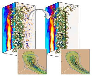
  $(2.86D)$ downstream of the nozzle, as shown in figure 1. This domain is typical for tomo-PIV and 4D-PTV measurements but far from sufficient for conventional numerical simulations as the inflow and outflow boundary conditions affect the flow. It is noted that the DA domain is selected to be slightly smaller than the virtual measurement domain mentioned in § 3.2 for ease of grid interpolation. The grid used in DA is Cartesian with 256, 128 and 128 elements uniformly distributed along the x, y and z directions, respectively, yielding a total of 4.36 million nodes with a spatial resolution of approximately 400 μm. This grid resolution meets the requirement of LES but does not enable reliable flow predictions owing to the undersized domain and inappropriate boundary conditions. The observations are produced by linearly interpolating (as expressed by
  $\mathrm{\mathbb{H}}$ (2.3)) the LES or tomo-PIV data onto the whole DA grid with a time interval
  $\mathrm{\Delta }T$. Boundary conditions, differential schemes and step lengths are applied according to the discussion in § 2.3.

Figure 1. Schematic of the computational domains. The large region denotes the cylindrical LES domain whereas the white box indicates the cuboid DA domain. The z coordinate is directed outwards perpendicular to the paper as noted by ‘⊙’. Lengths  ${L_f}$ and
  ${D_f}$ are plotted using different scales without showing the full range.
The DA cases considered in this study are listed in table 1. Clear cases (1–3) have ideal conditions with clear LES data as observations, and the regularisation in the DA computation is thus turned off. Different window lengths are tested to evaluate the sampling rate of the observations for the STR reconstruction. Noisy cases (4–6) use the LES data with white-noise contamination and box filtering (3 × 3 × 3 elements on the DA grid) as observations for evaluation of the de-noising capability. The noise standard deviation is approximately  $0.3{U_0}$ as that used by Gillissen et al. (Reference Gillissen, Bouffanais and Yue2019), and is introduced by adding random numbers in the range of
  $[ - {A_{noise}},{A_{noise}}]$ to the LES data, where
 \begin{equation}{A_{noise}}(\boldsymbol{x}) = 0.6\textrm{max}(||\boldsymbol{u}(\boldsymbol{x})||,0.2).\end{equation}
The coefficient 0.6 is used to tune the noise standard deviation to the desired value, and the minimum value of 0.2 is used to produce the noise in the ambient flow. The DA-Tomo case (case 7) uses the tomo-PIV data  ${\boldsymbol{u}^{tomo}}$ as observations, whereas in the DA-SS case (8), small-scale coherent structures are injected into the tomo-PIV observations according to
 \begin{equation}{\boldsymbol{u}^{obs}}(t) = {\boldsymbol{u}^{tomo}}(t) + {\boldsymbol{u}^{LES}}(t^{\prime}) - \widetilde{\boldsymbol{u}^{LES}}(t^{\prime}).\end{equation}
Here,  ${\boldsymbol{u}^{LES}}$ represents the velocity in LES, where
  $\widetilde{\boldsymbol{u}^{LES}}$ is the box-filtered LES data on the DA grid with a filter size of 7 × 7 × 7 elements, which is close to the physical size of the tomo-PIV interrogation volume. The time
  $t^{\prime} = t + 0.5\ \textrm{s}$ is used to ensure that the injected small-scale structures are not correlated with the tomo-PIV fields. The DA-SSN case (case 9) is similar to DA-SS except that white noise defined by (3.2) is added for further verification. The time step of the computation (i.e. the time interval of the STR reconstructed fields) is fixed at
  $\Delta t = 0.001\ \textrm{s}$, while
  $\Delta T$ denotes the length of each DA window. Time T is the total physical time counting all the DA windows in each case.
Table 1. List of DA cases and parameters.

Time  $\mathrm{\Delta }t\textrm{ }( = 0.001\ \textrm{s})$ is the time step of the DA computation;
  $\mathrm{\Delta }T$ is the length of the DA window; T is the total physical time for all the DA windows.
All the computations are performed on a desktop computer with an Intel Xeon E-2144G quad-core processor and 64 G memory. The serial computation of each multi-window case (cases 4–9) takes approximately 78 hours to find the optimal solution including the initial and inflow conditions, with there being 1000 instantaneous fields within the total time of 1.0 s (50 DA windows). Multitask parallel computing is conducted by submitting four cases at the same time to accelerate the overall computation by a factor of more than 3. The data writing is the most time-consuming step and further improvements can thus be made through the appropriate compression of the result files rather than writing ASCII data directly as done presently.
4. Results and discussion
4.1. Super-temporal-resolution reconstruction with down-sampled observations
Data assimilation is first applied for STR reconstruction using the observations of down-sampled LES data containing many small-scale turbulence structures. The computational cases are listed as cases 1–6 in table 1. The length of the intermediate DA window  $20\Delta t$ equals 100 LES time steps. For cases 4–6, 50 DA windows are computed within a total time T corresponding to 9 turnovers of the largest-scale mode (Hussain & Zaman Reference Hussain and Zaman2006) according to the Strouhal number St = 0.3. Figure 2 presents the iteration residuals for different step-length strategies in clear and noisy cases. In the initial field DA phase as shown in figure 2(a), the instantaneous flow at a random instant is used as the first guess. The adaptive step lengths are computed using (2.19a,b). The residual has an increasing descent rate with respect to the initial step length, with only 10 iterations required using
  $\lambda _{\boldsymbol{s}}^0 = 500$. Nevertheless, the residual grows rapidly after reaching a minimum when a constant step length is used; this growth is well suppressed by the adaptive formulation. In the model-error DA phase as shown in figure 2(b), there is an increasing descent rate with respect to the initial step length. When adopting the adaptive scheme, a gradual increase in the step length according to (2.20a) is effective in accelerating convergence whereas a large step length is prone to cause divergence. This problem can be solved using the adaptive step length with the combined use of (2.20a) and (2.20b). Although this adaptive scheme relies on trial and error to determine the optimal initial step length, the complementary computations can be performed only in the first time step or the first DA window, yielding an increase in the computational cost of less than 1 % in total in this study. In noisy cases, the residual gradient with respect to the iteration number is better suited to convergence evaluation as the residual level is strongly associated with the regularisation coefficient
  $\alpha $. Obviously, larger
  $\alpha $ results in better de-noising effects in the DA procedure and thus greater discrepancy between the DA results and observations. As shown in figure 2(c), the residual gradient has the highest convergence speed in the DA-Noisy5e-5 case, reducing to below 10−5 after 10 rounds of iteration. The number of iterations is fixed at 50 in the model-error DA phase of all noisy cases.

Figure 2. Residuals and their gradients in DA computations: (a) initial field DA, (b) model error DA in the case of DA-Clear30 and (c) residual gradients in the model error DA of noisy cases.
In the STR reconstruction, the flow at the middle instant between the two observations is undoubtedly subject to the largest reconstruction error. This suggests the need to inspect the reconstructed flow snapshot at the middle instant in the case of DA-Clear30 as shown in figure 3. The clear LES data and the POD optimal reconstruction (Appendix C) from the down-sampled observations with time interval  $30\mathrm{\Delta }t$ are also presented for comparison. The DA result is similar to the LES data on both longitudinal and cross-section planes as shown in figure 3(a–d). There are also slight differences in the upstream region near the inflow boundary, where some plume-like signatures are missing from the jet mainstream in the DA results. This is largely due to the error in the assimilated inflow conditions. In addition, the temporal evolution of these reconstructed fields shows the advantage of DA in STR reconstruction compared with interpolation-based approaches, which basically rely on temporally resolving the turbulence events with a sampling rate up to that meeting the Nyquist law. A POD full mode reconstruction (reconstruction using all of the modes) using the existing observations disrupts the real evolution process of the convecting small-scale vortices and is thus applicable only to slowly evolving vortices. A POD optimal reconstruction, as shown in figure 3(e,f), selects the most energetic modes that are temporally correlated for interpolation. This correctly recovers the flow convective properties but preserves less than 90 % of the total kinetic energy.

Figure 3. Instantaneous flow fields at the middle instant in the DA window: (a,b) DA reconstruction, (c,d) clear LES data and (e,f) POD optimal reconstruction. (a,c,e) The longitudinal middle sections and (b,d,f) the cross-sections at the location marked by the dashed line.
Figure 4 presents the pointwise error defined as
 \begin{gather}{\varepsilon _t} = {{\sum\limits_{(x,y,z)} {||\boldsymbol{u}(t) - {\boldsymbol{u}^{LES}}(t)||} } / {\sum\limits_{(x,y,z)} {||{\boldsymbol{u}^{LES}}(t)||} }},\end{gather}
 \begin{gather}{\varepsilon _x} = {{\sum\limits_{(t,y,z)} {||\boldsymbol{u}(x) - {\boldsymbol{u}^{LES}}(x)||} } / {\sum\limits_{(t,y,z)} {||{\boldsymbol{u}^{LES}}(x)||} }},\end{gather}
for each reconstruction scheme in clear cases. The summations are applied for all possible coordinates  $(x,y,z)$ and
  $(t,y,z)$, respectively. In this application, the terminal observation is fixed at
  $t/\Delta t = 30$ whereas the initial observations are selected at
  $t/\Delta t = 0$, 10 and 20 for the cases of DA-Clear30, DA-Clear20 and DA-Clear10, respectively. The direct simulation by solving the NS equation for the initial field at
  $t/\Delta t = 0$ yields an error that increases monotonically with respect to time, as shown in figure 4(a). This error is largely induced by the boundary conditions imposed on the compact numerical domain and is absorbed by the model error in this study. Data assimilation is performed from each selected initial field and yields the largest error at the middle time of the DA window before reaching a minimum at the end. The error is slightly higher than zero at each start and end time owing to the finite residual level at the final iterative loop. With assimilation of the model error
  $\boldsymbol{\xi }$, the error of the DA reconstruction is appreciably lower than that of the direct simulation and maintains a clear descending trend with respect to the decreasing DA window length
  $\Delta T$. Additionally, the POD full modes and optimal reconstructions are compared with the DA results for each corresponding observational time interval. As the full mode reconstruction at an observational time (start or end of the DA window) produces the exact fields, the error is reduced to zero. However, the reconstruction error at the intermediate instants remains much higher than that of the DA results for each window length. The POD optimal reconstruction reduces the maximum error for large observational time intervals but performs even worse than the POD full mode reconstruction for small time intervals. The above results indicate that although POD reconstruction plays important roles in the feature recovery of large-scale evolution, the lack of temporal information on small scales in the raw observations remains a barrier for the temporal resolution enhancement of turbulence details. In the DA reconstruction, the error is mainly concentrated in the upstream region, where the jet speed is high, as shown in figure 4(b); the error is manifested as the convection lag of the flow events, as shown by the instantaneous vertical velocity distributions. In addition, the inflow and outflow boundary conditions have notable local effects. Nevertheless, most of the error is below 1 % in the case of DA-Clear30, indicating the high accuracy of the proposed DA scheme for STR reconstruction even with a long time interval.

Figure 4. Pointwise error of the reconstructed flow in each clear case: (a) domain integration at different instants and (b) cross-wise and temporal integrations at different downstream locations. Instantaneous vertical velocities are inset in (b) for comparison.
As an analogy to the measurement noise in a real experiment (e.g. PTV), the noisy observations are synthesised by adding white noise to the clear LES data according to (3.2) and box filtering using 3 × 3 × 3 elements on a DA grid. In these cases, DA is performed successively in 50 windows using the terminal fields of the previous window for initialisation. Detailed parameters are given in table 1. To assess the accuracy of the DA field throughout the domain, the cross-correlation coefficient for the streamwise velocity is calculated using the clear LES data as reference for each instant in the DA window:
 \begin{equation}{C_x}(t) =
\frac{{\sum\limits_{\boldsymbol{x}}
{[u(\boldsymbol{x},t)\boldsymbol{\cdot
}{u^{LES}}(\boldsymbol{x},t)]} }}{{\sqrt
{\sum\limits_{\boldsymbol{x}} {{{[u(\boldsymbol{x},t)]}^2}}
\boldsymbol{\cdot }\sum\limits_{\boldsymbol{x}}
{{{[{u^{LES}}(\boldsymbol{x},t)]}^2}} }
}},\end{equation}
\begin{equation}{C_x}(t) =
\frac{{\sum\limits_{\boldsymbol{x}}
{[u(\boldsymbol{x},t)\boldsymbol{\cdot
}{u^{LES}}(\boldsymbol{x},t)]} }}{{\sqrt
{\sum\limits_{\boldsymbol{x}} {{{[u(\boldsymbol{x},t)]}^2}}
\boldsymbol{\cdot }\sum\limits_{\boldsymbol{x}}
{{{[{u^{LES}}(\boldsymbol{x},t)]}^2}} }
}},\end{equation}
where  $t \in [{t_0},{t_0} + \Delta T]$, and the summations are applied for each spatial location
  $\boldsymbol{x} = (x,y,z)$ on the DA grid. The cross-correlation coefficients for other velocity components are defined similar to (4.3). The final cross-correlation coefficients are averaged for each relative time with respect to the start instants in all the DA windows. The correlation coefficients for all the noisy cases, as well as the noisy observations, are shown in figure 5. The correlation coefficients of the noisy observations remain appreciably lower than those of all the DA cases owing to the noise contamination. This clearly indicates the strong capacity of DA to recover the turbulence properties even when taking noisy measurement data as observations. Comparatively, the regularisation term in the objective function not only eliminates noise but also plays an important role in improving the facticity of the reconstructed flow fields. The correlation coefficient is the highest at the middle instant of the DA window for the cases of DA-Noise5e-6 and DA-Noise5e-7 owing to the propagation of the governing equations. This trend is obviously different from that of the clear cases, where the error is largest in the middle of the window. When a smaller value of
  $\alpha $ is used, DA applies a larger weighting to the noisy observational data and thus introduces more error into the instantaneous field near the initial and terminal instants. We thus observe straighter correlation lines along time with larger
  $\alpha $, and the best performance with nearly constant correlations in the DA window is achieved in the case of DA-Noise5e-5. The optimal
  $\alpha $ is not readily obtained from figure 5 for different DA cases. The value of
  $\alpha $ is obviously case-dependent but can be cheaply determined adopting the DA procedure with only one window. In the remaining discussion of noisy cases, only DA-Noise5e-5 is taken as the representative example.

Figure 5. Cross-correlation coefficients of the reconstructed velocity fields with the referential LES data: (a) x component, (b) y component and (c) z component. The noisy LES data are averaged over all time. Different ordinate scales are used for clear illustration.
The assimilated  $\boldsymbol{\xi }$ term acts as a compensator of error between the model prediction and observation. It also plays an important role in the turbulence evolution. The physical interpretability of the compensator has increasingly drawn attention for numerous data-driven techniques. The compensator not only directly reduces the predictive error between two datasets but also is a feature vital for the flow to evolve correctly. Term
  $\boldsymbol{\xi \; }$ has equivalent effects on flows with pressure gradients in the NS equations but is always divergence-free according to (2.17). Helmholtz decomposition casts
  $\boldsymbol{\xi \; }$ in two parts as
 \begin{equation}\boldsymbol{\xi } = \boldsymbol{\psi } - \boldsymbol{\nabla }\varphi ,\end{equation}
where  $\boldsymbol{\psi }$ is stochastic forcing due to, for example, the subgrid stress. The reconstruction error is included in
  $\boldsymbol{\psi }$ in the present DA framework. Term
  $\boldsymbol{\nabla }\varphi $ is the irrotational part, which is lumped into the pressure gradient. The pressure and pressure gradient component in the x direction are first explored in figure 6. There is a visible difference in the pressure and its gradient distributions between the clear LES result and the other results. Simulation by solving the original NS equations directly does not reproduce the pressure and gradient correctly, as shown in figure 6(a–d). The quantitative comparison presented in figure 7 shows the model error effects on the confined computational domain. The results obtained by simulation and DA have high similarity, as shown in figure 6(c–f), with only slight discrepancy observed quantitatively in figure 7. The above results demonstrate the important contribution of the irrotational part
  $\boldsymbol{\nabla }\varphi $ in compensating for the pressure gradient discrepancies stemming from the compact computational domain. The results also indicate that further computation steps after DA are required to reconstruct the pressure fields correctly. An explicit calculation of
  $\boldsymbol{\nabla }\varphi $ and
  $\boldsymbol{\psi }$ can be readily made considering the difference in the pressure gradients between the LES and DA, i.e.
 \begin{gather}\boldsymbol{\nabla }\varphi = \boldsymbol{\nabla }{p^{LES}} - \boldsymbol{\nabla }{p^{DA}},\end{gather}
 \begin{gather}\boldsymbol{\psi } = \boldsymbol{\xi } + \boldsymbol{\nabla }{p^{LES}} - \boldsymbol{\nabla }{p^{DA}}.\end{gather}
Probability density functions (PDFs) of  ${\xi _x}$,
  ${\psi _x}$ and
  ${\nabla _x}\varphi $ are plotted in figure 8, where
  ${\nabla _x}$ is the streamwise component of the gradient. All quantities are normalised by
  $U_0^2/D$. Herein, PDFs are separately calculated for all DA windows at the second instant immediately after the initial time (figure 8a), at the middle instant (figure 8b) and at the terminal instant (figure 8c) using data in the region
  $r/D < 1$ (where
  $r = \sqrt {{y^2} + {z^2}} $). The results of averaging across all instants are shown in figure 8(d). The curves for the negative part of the abscissa are mirrored to the positive part to demonstrate the asymmetry with respect to the ordinate axis. The PDFs of
  ${\xi _x}$ have a sharp peak at the origin and rapidly decay in both positive and negative directions of the abscissa. There are clear differences between the positive and negative bunches, especially at the first instant, as shown in figure 8(a). This indicates that
  ${\xi _x}$ has a pronounced bias towards the positive direction and complements the pressure gradient from the perspective of the whole region of interest. Recalling that direct simulation yields a lower speed of convection in the downstream direction as depicted in figure 4(b),
  ${\xi _x}$ is physically interpreted as the driving force for the model prediction to keep up with the observation evolution. However, the importance of the driving force varies in time and largely prevails in the first half of the DA window. This depends on
  ${\nabla _x}\varphi $, which is biased against the driving force. The PDFs of
  ${\xi _x}$ and
  ${\nabla _x}\varphi $ averaged across all the instants and shown in figure 8(d) clearly demonstrate the above mentioned complementation mechanism during the flow evolution in the DA window, although there is slightly anomalous behaviour at the terminal instant in figure 8(c), probably due to computational error. Supplemental evidence for this supposition is provided by the PDFs of
  ${\psi _x}$, which show good agreement for the positive and negative bunches at each instant in the figure. This result is consistent with our previous conjecture as the remaining part of
  ${\xi _x}$, when subtracting the irrotational part
  $\boldsymbol{\nabla }\varphi $, has unbiased stochastic behaviours that are responsible for the production and dissipation of turbulence.

Figure 6. Instantaneous pressure (a,c,e) and streamwise-component pressure gradient (b,d,f) fields in (a,b) clear LES, (c,d) simulation and (e,f) the case of DA-Noise5e-5.

Figure 7. Quantitative comparison of (a) the pressure and (b) its streamwise-component gradient along a streamwise line at  $y/D = 0.5$.

Figure 8. The PDFs of the quantities  ${\xi _x}$,
  ${\psi _x}$ and
  ${\nabla _x}\varphi $ at (a) the second instant, (b) the middle instant, (c) the terminal instant and (d) all instants. The data on the negative abscissa are mirrored to be positive. Here
  $\varTheta $ denotes
  ${\xi _x}$,
  ${\psi _x}$ or
  ${\nabla _x}\varphi $ as indicated by the arrows.
A direct view of the STR reconstruction is acquired from figure 9, where the temporal variations of the original and reconstructed velocities are plotted. The streamwise velocities at  $x/D = 3.5D$ on the jet centreline are quantitatively compared in figure 9(a). The rapid variation of the clear LES results represents the small-scale coherent structures in the jet turbulence. The down-sampling of the observations (‘Noisy LES obs.’) only captures the large-scale events even when adopting spline interpolation, and the observational noise induces appreciable deviation from the clear LES data. However, the DA results recover the small-scale fluctuations well, even though slight discrepancies are still observed. A salient feature of DA is that the STR results do not strictly follow the variation of the observations, manifesting remarkable de-noising and correcting effects when erroneous observations are used. The spatiotemporal plots of the streamwise velocities at the cross-section
  $x/D = 3.5D$ are present in figure 9(b–d). The clear LES data in figure 9(b) reveal appreciable temporal fluctuations along with the small-scale variation showing apparent coherent tubular structures. The detailed small vortex organisations are seen in the vorticity contours. In the down-sampled observations shown in figure 9(c), although a smooth isosurface is obtained, the loss of details between successive snapshots is an issue. This situation is equivalent to direct temporal interpolation, which makes sense only when the original sampling frequency meets the requirement of the Nyquist sampling law. The DA reconstruction shows obvious advantages in the recovery of flow details even when using the noisy down-sampled observations. The DA results with the sampling rate equalling that of the clear LES data are shown in figure 9(d). The contours of the streamwise vorticity clearly demonstrate the reconstructed flow details. The red circles mark the moderate-scale vortices that exist in the clear LES data and are successfully reconstructed by DA but are lost in the down-sampled observations.

Figure 9. Temporal plots of the velocity and vortical structures (Q = 500) from the original and DA reconstructed flow fields at  $x/D = 3.5D$: (a) streamwise velocity variation on the jet centreline, (b) clear LES data with the time interval
  $\Delta t = 0.001\ \textrm{s}$, (c) noisy LES observations with the time interval
  $\Delta T = 0.02\ \textrm{s}$, (d) STR reconstructions with the time interval
  $\Delta t = 0.001\ \textrm{s}$. The green dots and the dashed line in (a) denote the observational data and the spline fitting, respectively. The black dashed lines in (b–d) indicate the observational instants.
In-depth analysis of the small scales recovery of DA is conducted using the velocity spectra. Power spectral densities (PSDs) are computed using Welch's method (Welch Reference Welch1967) with all 1000 snapshots for each case. Although the window size of 200 (corresponding to 1.8 turnovers of the largest-scale flow fluctuation) with an overlap of 100 in the PSD computation does not provide a good estimation of the spectra at low frequencies due to the data size, the results are not visibly different from those obtained using larger windows. Our present analysis focuses on high-frequency structures with Strouhal numbers larger than 0.2, which can be well captured by the present PSD algorithm. Figure 10 shows the PSDs of the streamwise velocity at various radial locations. The PSDs of the time-sparse noisy LES data are lower than the others due to the normalisation using the root mean square of the velocity signals, and it is only possible to resolve vortical structures up to  $St = 0.1$ with a relatively flat distribution due to the noise. The POD optimal reconstruction recovers the large-scale vortices well but yields a rapid decay of the PSDs at
  $St > 0.5$ due to the lack of small-scale information. The DA reconstruction produces the best results up to
  $St = 5$, although with a plateau higher than that for the clear LES data due to the noise in the observations. An observable feature of the PSDs at different radial locations is the underestimation of the DA reconstruction at
  $r/D = 0$ but a slight overestimation at
  $r/D = 1.5$. This feature is reasonable in the present computations due to the high noise ratio at far radial locations where the flow speed is low.

Figure 10. PSDs on the streamwise velocity at the downstream position  $x/D = 3.5D$ at various radial locations: (a)
  $r/D = \textrm{0}$, (b)
  $r/D = 1$ and (c)
  $r/D = 1.5$.
4.2. Super-temporal-resolution reconstruction for tomo-PIV with small scales injection
Although tomo-PIV has become one of the most widely used volumetric measurement techniques in fluid mechanics, the compromise between the measurement domain size and the spatial resolution resulting from the cross-correlation (Lawson & Dawson Reference Lawson and Dawson2014; Naka et al. Reference Naka, Tomita, Shimura, Fukushima, Tanahashi and Miyauchi2016; Fiscaletti et al. Reference Fiscaletti, Ragni, Overmars, Westerweel and Elsinga2022) is the major issue that limits its application in certain circumstances. The present study evaluates the field correction for the low-sampling-rate tomo-PIV results through DA reconstruction, with much effort being given to the regeneration of the turbulence structures by small scales (SS) injection from the observations. It is worth noting that the small vortices cannot be injected from the initial condition as done by Li et al. (Reference Li, Zhang, Dong and Abdullah2019) because of the weak-constraint nature of the present DA algorithm and the time-sparse observations.
The case of DA-Tomo (see table 1) is first discussed on the basis of the snapshots selected at the terminal instant of the DA window. The comparison of the tomo-PIV data (observation) and the DA result presented in figure 11(a,b) shows excellent similarity in terms of the velocity contours and even the three-dimensional vortical structures (Q-criterion isosurface, Q = 500). However, a notable feature of the DA procedure is the prominent ability to remove the velocity divergence error, which is important for post-processing, such as vorticity computation and pressure determination, using the existing three-dimensional fields. A snapshot obtained by box filtering (denoted  $\widetilde {\boldsymbol{u}^{LES}}$, filtered using 7 × 7 × 7 elements on the DA grid, which is close to the physical size of the tomo-PIV interrogation volume) from the clear LES data at a selected instant is shown in figure 11(c). The velocity contours barely show any difference between the different data, but the isosurface of the Q criterion in the box-filtered field is more coherent with many elongated vortex tubes distributed in the jet shear layer. This indicates that the cross-correlation process in tomo-PIV measurements involves far more than spatial filtering than what has been commonly understood before, and more complex effects should be considered.

Figure 11. Instantaneous velocity fields and vortical structures  $(Q = 500)$ of (a) the synthetic tomo-PIV measurements, (b) DA reconstruction and (c) filtered LES data on the DA grid.
The turbulence fields of the reconstructed flow can be inspected in more depth by plotting the joint PDFs of the invariants  ${Q^\ast }$ and
  ${R^\ast }$, which are defined as (Rishita & Girimaji Reference Rishita and Girimaji2022)
 \begin{gather}{Q^\ast } =- {\textstyle{1 \over 2}}{b_{ij}}{b_{ji}},\end{gather}
 \begin{gather}{R^\ast } =- {\textstyle{1 \over 3}}{b_{ij}}{b_{jk}}{b_{ki}},\end{gather}
where  ${b_{ij}} = {A_{ij}}/||A||$. Here, the asterisk is added to the invariants to distinguish them from the vortex Q criterion. The velocity gradient tensor is
  ${A_{ij}} = \partial {u_i}/\partial {x_j}$, and
  $||\cdot ||$ denotes the Frobenius norm. The zero-discriminant lines are determined according to
  ${Q^{{\ast} 3}} + 27{R^{{\ast} 3}}/4 = 0$. It has been well established that the
  ${Q^\ast }$–
 ${R^\ast }$ PDFs have a characteristic teardrop shape (i.e. a Vieillefosse tail) (Vieillefosse Reference Vieillefosse1984) in various turbulent flows, with a high probability of occurrence along the right discriminant line. This characteristic probability map represents the predominance of sheet-like structures in the fourth quadrant and that of vortex stretching in the second quadrant. In this study,
  ${Q^\ast }$–
 ${R^\ast }$ maps are calculated using all the flow instantaneous fields in the region of
  $r/D < 0.75$. A map of the clear LES data is plotted using solid contours in each panel of figure 12 for comparison. Figure 12(a) shows that both the clear and filtered LES data have the well-known teardrop shape in the
  ${Q^\ast }$–
 ${R^\ast }$ plane, whereas the filtered flow has a slightly slimmer tail indicating fewer sheet-like structures and less vortex compression effects. However, there is an appreciable difference in the tomo-PIV data, where the predominant occurrences of the high PDFs are located slightly above the discriminant lines, as shown in figure 12(b). Misalignment in tomo-PIV data has previously been observed (Khashehchi et al. Reference Khashehchi, Elsinga, Ooi, Soria and Marusic2010) but with high PDFs slightly below the discriminant lines. This misalignment is obviously case-dependent, whereas tomo-PIV invariably fails to capture the detailed turbulence dynamics. The DA reconstruction produces a
  ${Q^\ast }$–
 ${R^\ast }$ map having a well-organised teardrop shape, which is shown in figure 12(c) and is more like the filtered LES results. This implies an improvement of the DA procedure in turbulence reconstruction even though the improved reconstruction can be hardly distinguished from the vortical structures, as shown in figure 11. Additionally, there is a slight difference, with a sharper Vieillefosse tail, relative to both the clear and filtered LES data. In contrast, Vieillefosse tails were observed to be shorter and blunter in the work of Li et al. (Reference Li, Zhang, Dong and Abdullah2019) owing to the use of different DA algorithms.

Figure 12. Joint PDFs of the velocity gradient invariables  ${Q^\ast }$ and
  ${R^\ast }$. The solid contours show the clear LES data, while the coloured dashed lines show (a) filtered LES results, (b) tomo-PIV data and (c) the DA reconstruction. White dashed lines in the third and fourth quadrants represent the zero-discriminant lines
  ${Q^{{\ast} 3}} + 27{R^{{\ast} 3}}/4 = 0$. The PDFs are normalised by the mean values on the
  ${Q^\ast }$–
 ${R^\ast }$ plane.
The filtered flow  $\widetilde {\boldsymbol{u}^{LES}}$ is then subtracted from the clear LES fields to derive the small-scale structures, which can be added to the tomo-PIV observations for the SS injection. To remove the correlation between the injected small scales and the tomo-PIV snapshots, a time shift of 0.5 s (approximately 4.5 turnovers of the largest-scale jet oscillation) is applied for the observations in the cases of DA-SS and DA-SSN. This approach is analogous to real tomo-PIV work where small-scale information is injected from independent numerical data. Recalling that the SS injection from initial fields is subject to extremely expensive computation, taking 15 days to determine a single initial field in a long DA window as noted by Li et al. (Reference Li, Zhang, Dong and Abdullah2019), the observation injection in the present study requires less than 5 minutes to determine each optimal field on a desktop computer, with the number of computational grid elements being twice that used by Li et al. (Reference Li, Zhang, Dong and Abdullah2019). This SS injection is principally achieved by the adjoint source, which transfers the large-scale information from the observations to the primary flow quantities, with the system equations serving as the physical filter for the vortex correction and noise removal. A qualitative understanding of the DA reconstruction for small scales recovery is acquired from figure 13, which presents different observations and the DA results. It is noted that the Q value (3000) used to show the three-dimensional vortical structures is much larger than that used for figure 11. The tomo-PIV field and its DA result in figure 13(a,d) thus show few vortical structures and a low vorticity magnitude with much emphasis on the small scales in the cases of SS injection. Recalling that the regularisation coefficient
  $\alpha $ is selected to minimise the difference between the mid-time and terminal-time reconstructed fields and for de-noising in noisy cases, the DA reconstructions in figure 13(e,f) have a certain attenuation of the vorticity magnitude relative to the observations in figure 13(b,c) but are still considerably higher than those in the tomo-PIV field. These results are clear demonstrations of SS injection, with small-scale structures regenerated in the DA fields differing from those in the observations. The authenticity of these reproduced small-scale turbulence dynamics is thus evaluated subsequently.

Figure 13. Instantaneous vorticity magnitude contours and vortical structures (Q = 3000) of the observations (a–c) and DA reconstructions (d–f): (a) tomo-PIV observation, (b) tomo-PIV observation with SS injection, (c) tomo-PIV observation with SS injection and noise, (d) DA-Tomo, (e) DA-SS and (f) DA-SSN. The instant at the terminal of a DA window is taken.
The joint PDFs of the invariants  ${Q^\ast }$ and
  ${R^\ast }$ of the observations and DA results are shown in figure 14. These invariant maps are computed according to (4.7) and (4.8). The invariant map of the clear LES data is plotted in each panel for comparison. It is observed that with SS injection, the tomo-PIV generates the teardrop shape of the invariant map much better than the original measurements (figure 14a). The Vieillefosse tails shift onto the right discriminant line but are still shorter than those of the clear LES data. The noise greatly deteriorates the map pattern such that the characteristic teardrop shape is not seen, as shown in figure 14(b). The induced error is prone to raise the high-PDF regions in the third and fourth quadrants above the discriminant lines, which is also seen in the original tomo-PIV data in figure 12(b). Despite the unphysical turbulence in the observations, DA is able to improve the dynamical feature substantially, resulting in the well-organised teardrop shapes of PDFs on the
  ${Q^\ast }$–
 ${R^\ast }$ plane as shown in figure 14(c,d).

Figure 14. Joint PDFs of the velocity gradient invariables  ${Q^\ast }$ and
  ${R^\ast }$. The solid contours show the clear LES data, while the coloured dashed lines show (a) tomo-PIV observations with SS injection, (b) tomo-PIV observations with SS injection and noise, (c) the case of DA-SS and (d) the case of DA-SSN. White dashed lines in the third and fourth quadrants represent the zero-discriminant lines
  ${Q^{{\ast} 3}} + 27{R^{{\ast} 3}}/4 = 0$. The PDFs are normalised by the mean value on the
  ${Q^\ast }$–
 ${R^\ast }$ plane.
An important feature of velocity gradients in turbulence flows is the alignment of the vorticity along the eigenvectors of the strain-rate tensor  ${S_{ij}}$ (Ashurst et al. Reference Ashurst, Kerstein, Kerr and Gibson1987). This alignment largely determines the vortex stretching term
  ${S_{ij}}{\omega _i}{\omega _j}$, which is the main source of the enstrophy growth. By examining the PDFs of the cosines of angles between the vorticity vector and the eigenvectors of
  ${S_{ij}}$ (i.e.
  $|{\hat{\boldsymbol{e}}_1}\boldsymbol{\cdot }\hat{\boldsymbol{\omega }}|$,
  $|{\hat{\boldsymbol{e}}_2}\boldsymbol{\cdot }\hat{\boldsymbol{\omega }}|$ and
  $|{\hat{\boldsymbol{e}}_3}\boldsymbol{\cdot }\hat{\boldsymbol{\omega }}|$, where the eigenvectors
  ${\hat{\boldsymbol{e}}_1}$,
  ${\hat{\boldsymbol{e}}_2}$ and
  ${\hat{\boldsymbol{e}}_3}$ are arranged in descending order of the corresponding eigenvalues
  ${\lambda _1} > {\lambda _2} > {\lambda _3}$, and
  $\hat{\boldsymbol{\omega }}$ denotes the normalised vorticity vector), the preferential alignment of
  $\hat{\boldsymbol{\omega }}$ with
  ${\hat{\boldsymbol{e}}_2}$ is observed. Checking the vorticity alignments in the different fields provides a useful means for assessing the effectiveness of the DA scheme in recovering the turbulence dynamic features. Figure 15 shows that the alignment of the vorticity vector with each eigenvector in the clear LES data has a tendency similar to that in a turbulent jet, as shown by Buxton & Ganapathisubramani (Reference Buxton and Ganapathisubramani2010), and to that in spatially developing flow, as shown by Gomes-Fernandes, Ganapathisubramani & Vassilicos (Reference Gomes-Fernandes, Ganapathisubramani and Vassilicos2014), with the preferential alignment of the vorticity being along the second eigenvector. For other data in figure 15, there are certain discrepancies of the alignments compared with the clear LES. The vorticity alignments in the case of DA-tomo-PIV have a tendency almost identical to that of the original tomo-PIV results except for the third eigenvector, where there is a slight improvement, as shown in figure 15(c). This suggests that the DA procedure hardly changes the vortex orientation when using the tomo-PIV data as observations due to an absence of small-scale vortices. The SS injection improves the vorticity alignment with the first eigenvector, as shown in figure 15(a), whereas the case of DA-SS further augments the alignments with the second and third eigenvectors, as shown in figure 15(b,c). We see here evidence for the dynamic feature enhancement of small-scale turbulence structures; this is more conspicuous when there is noise in the observations, as the alignment is improved substantially in the case of DA-SSN from a rather poor tendency in the noisy observations.

Figure 15. Alignment of the vorticity vectors with the eigenvectors of the strain-rate tensor. (a) Alignment with the first (extensive) eigenvector, (b) alignment with the second (intermediate) eigenvector and (c) alignment with the third (compressive) eigenvector. The ordinate scales differ across panels.
Another important feature of turbulence flows is the modulation of the small-scale vortices by the large-scale gradients. Many studies have shown that large-scale structures modulate small scales both in amplitude and frequency (Mathis, Hutchins & Marusic Reference Mathis, Hutchins and Marusic2009; Ganapathisubramani et al. Reference Ganapathisubramani, Hutchins, Monty, Chung and Marusic2012; Fiscaletti, Ganapathisubramani & Elsinga Reference Fiscaletti, Ganapathisubramani and Elsinga2015) rather than the scales being independent of each other as had long been considered. In jet flows, the small-scale signal has a stronger amplitude for positive fluctuations of the large-scale signal independently of the radial location (Fiscaletti et al. Reference Fiscaletti, Ganapathisubramani and Elsinga2015). There is also preferential alignment between the vorticities on the small and large scales, indicating that the vorticity direction does not vary appreciably across the scales (Fiscaletti et al. Reference Fiscaletti, Attili, Bisetti and Elsinga2016). This body of research suggests that the anisotropy of the large scales is partially preserved at the small scale, which seems to be in contrast with the local isotropy hypothesis (Pope Reference Pope2000). The small scales have been defined to be smaller than the Taylor length scale  ${\lambda _T}$. Fiscaletti et al. (Reference Fiscaletti, Attili, Bisetti and Elsinga2016) reported that the scale modulation was weakened at larger scales but remained appreciable at scales up to
  $3{\lambda _T}$. Inspection of the scale modulation of the DA results is thus important in evaluating the DA scheme on the accurate recovery of the scale organisation in the cascade mechanism.
Following Fiscaletti et al. (Reference Fiscaletti, Attili, Bisetti and Elsinga2016), the amplitude modulation is assessed by defining the local vorticity root mean square  $A_{gL}^\ast $ and the large-scale velocity gradient
  $g_L^\ast $ as
 \begin{gather}A_{gL}^\ast (\boldsymbol{x}) = \sqrt {\frac{1}{N}\sum\limits_{i = 1}^N {(||{\boldsymbol{\omega }_i} - \tilde{\boldsymbol{\omega }}||)} } ,\end{gather}
 \begin{gather}g_L^\ast (\boldsymbol{x}) = \frac{1}{N}\mathop \sum \limits_{i = 1}^N \sqrt {\left. {\frac{{\partial {{\tilde{u}}_x}}}{{\partial y}}} \right|_i^2 + \left. {\frac{{\partial {{\tilde{u}}_x}}}{{\partial z}}} \right|_i^2 + \left. {\frac{{\partial {{\tilde{u}}_y}}}{{\partial x}}} \right|_i^2 + \left. {\frac{{\partial {{\tilde{u}}_y}}}{{\partial z}}} \right|_i^2 + \left. {\frac{{\partial {{\tilde{u}}_z}}}{{\partial x}}} \right|_i^2 + \left. {\frac{{\partial {{\tilde{u}}_z}}}{{\partial y}}} \right|_i^2} .\end{gather}
Here,  $A_{gL}^\ast $ is a measure of small-scale vortical structures whereas
  $g_L^\ast (\boldsymbol{x})$ only includes the shear components of the large-scale velocity gradients. Both quantities are normalised by the corresponding mean values. The tilde denotes the large-scale quantities in each dataset, and N is the number of nodes in the filtering window where the large scales are computed. Herein, the definition of large scales is not straightforward, as simply imposing filters does not give a reasonable and clear separation of the different scales in the present jet. In the clear LES, noisy LES and DA-Noisy5e-5 results, the filtered LES results obtained using a filter size of 7 × 7 × 7 elements on the DA grid (as shown in figure 11c) are taken as the large scales. The tomo-PIV original data are used as large scales for observations of SS injection and SS injection with noise. In the DA-SS and DA-SSN cases, the DA-Tomo results are used as large scales. With these definitions, the filter size is estimated to be approximately
  $3{\lambda _T}$ using the dissipation formulation of (3.1), and the scale modulation should still be appreciable according to the above discussion. Statistics of the activity at small scales conditioned on the large-scale gradients are shown in figure 16(a). Computations are performed in the region of
  $r/D \le 0.75$. The results show that the clear LES results have a nearly linear correlation as obtained by Fiscaletti et al. (Reference Fiscaletti, Attili, Bisetti and Elsinga2016) for
  $0.5 < g_L^\ast < 2.5$. This confirms that large-scale gradients strongly modulate small-scale structures. Even with a high level of noise in observations with attenuated correlation (see ‘Noisy LES’), this modulation is substantially improved in the case of DA-Noisy5e-5. The accuracy of the modulation recovery by DA is indeed region-dependent, as much better recovery can be observed (not shown here) by checking only the jet shear layer region at
  $r/D \approx 0.5$. It is seen that in the case of DA-SS, there is notable improvement relative to the SS-injected observations even with temporally sparse observational data. A loss of the scale modulation in the SS injection with and without noise is expected as the large- and small-scale structures are fully uncorrelated. Data assimilation improves the modulation properties regardless of the observational noise. This modulation recovery is an important criterion with which to assess the DA scheme in the reconstruction of real turbulence even when the small-scale structures are synthetic or contaminated with noise in measurement applications.

Figure 16. Modulation and alignment of vortices at different scales. (a) Local vorticity root mean square  $A_{gL}^\ast $ conditioned on the fluctuations of the large-scale gradients
  $g_L^\ast $. (b) Alignment of large-scale vorticity vectors with small-scale vorticity vectors.
The modulation is also reflected in the vortex alignment between the small- and large-scale structures. The PDFs of the cosine of the angle between large and small scales (expressed as  $|{\boldsymbol{\omega }_L}\boldsymbol{\cdot }{\boldsymbol{\omega }_S}|$) are plotted in figure 16(b). It is seen that in the clear LES data, the small-scale vortices have a preferential alignment with the large-scale vortices, as demonstrated by the rapid increase in the PDFs as
  $|{\boldsymbol{\omega }_L}\boldsymbol{\cdot }{\boldsymbol{\omega }_S}|$ approaches 1. We also see that this alignment is almost fully recovered even with noisy observations in the case of DA-Noisy5e-5. There is nearly no alignment correlation of different scales in the observations of SS injection and that with noise, with PDFs being almost horizontal in the range of
  $0 \le |{\boldsymbol{\omega }_L}\boldsymbol{\cdot }{\boldsymbol{\omega }_S}|\le 1$. This is further evidence that the small- and large-scale structures are independent in the original SS-injected observations. However, the vortex alignment is clearly improved by DA with the PDFs increasing at large values of
  $|{\boldsymbol{\omega }_L}\boldsymbol{\cdot }{\boldsymbol{\omega }_S}|$.
4.3. Lagrangian particle tracking through STR reconstruction
One of the motivations of the present study on STR reconstruction is to establish an auxiliary role for the successive prediction of particle positions in 4D-PTV. Four-dimensional PTV relies on the successive tracking of densely distributed particles at different instants to form long trajectories. This greatly increases the spatial resolution of the velocity vectors and improves the measurement accuracy by eliminating ghost particles that exist in tomo-PIV measurements, when using the same instrument configuration. The shake-the-box (STB) technique (Schanz, Gesemann & Schrder Reference Schanz, Gesemann and Schrder2016) is a representative 4D-PTV technology that predicts the new particle positions after the trajectory initialisation, followed by position perturbation for the iterative correction. Physically constrained interpolation schemes are adopted to reconstruct velocity fields on an Euler grid (Gesemann et al. Reference Gesemann, Huhn, Schanz and Schroder2016; Schneiders & Scarano Reference Schneiders and Scarano2016). However, a high frequency of camera imaging (i.e. small displacements of the particles at two successive sampling instants) is required to identify the same particles in the image sequence (i.e. particle pairing) (Khojasteh et al. Reference Khojasteh, Yang, Heitz and Laizet2021). This requirement limits the use of the STB technique to low-speed flows for currently available measurement devices. Lagrangian particle tracking largely depends on the particle prediction for the next instant before the position correction (shaking). A Wiener filter (Wiener Reference Wiener1949) is used in the prediction phase of the STB technique, with the accuracy of prediction deteriorating drastically for short trajectories and large particle displacement (Schanz et al. Reference Schanz, Gesemann and Schrder2016). Although a multi-pulse strategy using more cameras and lasers overcomes this difficulty by equivalently increasing the sampling rate and thus reducing the particle displacement (Manovski et al. Reference Manovski, Novara, Mohan, Geisler and Schrder2021), we prefer less expensive methods based on STR reconstruction for artificially increasing the imaging frequency. This relies on the accurate recovery of the detailed turbulence between the two given snapshots, which can be tentatively determined by either tomo-PIV or conventional PTV using the double-exposure mode of the cameras. Although the practice of this measurement strategy is left as a topic of future study, Lagrangian particle tracking using the existing flow fields is evaluated here as a preliminary demonstration.
Once the velocity fields are obtained, the new particle position  ${\boldsymbol{x}_t}$ is computed from the previous position
  ${\boldsymbol{x}_{t - 1}}$ and previous local velocity
  ${\boldsymbol{u}_{t - 1}}$ as
 \begin{equation}{\boldsymbol{x}_t} = {\boldsymbol{x}_{t - 1}} + {\boldsymbol{u}_{t - 1}}\boldsymbol{\cdot }(\Delta t\ \textrm{or}\ \Delta T).\end{equation}
The time step of the DA computation  $\Delta t$ or the time interval of the observations (DA window length)
  $\Delta T$ is used in (4.11) depending on the data used in different cases. This particle tracking formulation neglects various forces exerted on the particles by the fluid or adjacent particles; i.e. particles are distributed at a certain distance from each other and fully follow the flow as required for particle seeding in 4D-PTV measurements. We assume that the terminal field has been iteratively corrected in real experiments but includes a certain level of error. This implies that the terminal field does not need to be strictly accurate in using the present STR reconstruction. The particle prediction using the field of POD optimal reconstruction (Appendix C) and the Wiener prediction (Schanz et al. Reference Schanz, Gesemann and Schrder2016; Tan et al. Reference Tan, Salibindla, Masuk and Ni2019) are evolved for comparison.
Prediction errors are evaluated at the terminal instants in different DA windows using the clear DA cases. This evaluation demonstrates the best prediction that the DA can achieve using the present STR reconstruction strategy. To compute the error, particles are initialised at different radial and streamwise locations before they are convected downstream until the terminal instant in the DA window. The errors are computed as the distance from the predicted particles to the true particles at the terminal instant, and they are normalised using the voxel size in the tomo-PIV measurement as mentioned in § 3.2. Figure 17 shows the azimuthally averaged prediction errors for different lengths of the DA window. The largest error is found to be 13 voxels in the upstream region when the window length  $\Delta T = 30\Delta t$ as shown in figure 17(a). This clearly demonstrates that the error decreases as the location moves downstream and the window size decreases. For a window length
  $\Delta T = 20\Delta t$ as shown in figure 17(b), the error is smaller than 6 voxels at all the considered locations, and the error becomes less than 2 voxels in the downstream half-domain when the window length is reduced to
  $\Delta T = 10\Delta t$ as shown in figure 17(c).

Figure 17. Particle prediction errors in the clear DA cases at the terminal instant: (a) window length  $\Delta T = 30\Delta t$, (b) window length
  $\Delta T = 20\Delta t$ and (c) window length
  $\Delta T = 10\Delta t$. Results are averaged in the azimuthal direction.
Particle prediction is performed for each DA window independently in noisy cases as shown in figure 18; i.e. the particles are moved to the true positions (black dots on the true track) at each initial instant and the errors are evaluated at the terminal instant in a DA window. Data assimilation needs only two flow snapshots to compute the track whereas the Wiener prediction requires at least four previous positions for track initialisation and many more historical positions for improved accuracy. At time  $t = 0$, two particles are initialised at
  $r/D = 0$ and
  $r/D = 0.5$ on the inflow surface. Figure 18(a) shows the seventh to the tenth true positions of the centreline particle. The true trajectory is computed using the clear LES data with time interval
  $\Delta t$ in (4.11), but the time interval between two successive black dots shown in figure 18(a) is
  $\Delta T = 20\Delta t$. The fifth-order Wiener prediction is applied using all the previous true positions with a time interval
  $\Delta T$, as we assume that only the down-sampled observations are known. It is seen that the Wiener prediction using the previous eight true positions determines the ninth position far from the truth; this also occurs for the prediction of the tenth position. The small red dots denote the DA prediction in the case of DA-Noisy5e-5 with short-time marching realised through STR reconstruction. This prediction is thus more accurate, being much closer to the true positions. Figure 18(b) presents the error evolution with time. It is seen that the error in the DA prediction decays with time as the particle convects downstream. The largest error is approximately 30 voxels in the upstream region. The error decay in the DA prediction is mainly due to the increase in accuracy of the STR reconstruction in the downstream region. The Wiener prediction has an error greater than 100 voxels in the upstream region and decays as more historical information becomes available. However, the error in the Wiener prediction remains higher than that in the DA prediction even at the last several instants. Indeed, the Wiener prediction improves when there are more historical data, but it is not applicable as the particles exit the measurement domain on excessively long trajectories. The DA procedure is thus preferable over the Wiener filter for particle prediction with long time intervals.

Figure 18. Particle prediction and position errors at different times: (a) three-dimensional tracking process and (b) errors at each terminal instant. The true track is computed using the clear LES data whereas the DA prediction is based on the case of DA-Noisy5e-5.
Figure 19 shows the particle prediction error for conditions closer to those of a real experiment subject to various flow measurement errors. The computational procedures are similar to those used in obtaining the results in figure 17 but involve further averaging across all the DA windows. The noisy LES and tomo-PIV results are computed using the time-sparse flow data with the time interval  $\Delta T = 20\Delta t$ as if the high-sampling-rate fields were not available, whereas all DA predictions use the time interval
  $\Delta t$. The case of DA-Clear20 is reproduced here as a lower bound for the present STR strategy, and the POD optimal reconstruction, which yields much higher particle error, is also shown for comparison. The particle prediction using the tomo-PIV fields, which has been widely used in conventional PTV algorithms, has errors larger than 15 voxels in most of the measurement domain. The DA predictions in the cases of DA-SS and DA-SSN have errors similar to the error in the tomo-PIV results, whereas the DA prediction in the case of DA-Tomo has slightly less error owing to the STR reconstruction with a much smaller time step. Among all the discussed DA approaches, the case of DA-Noisy5e-5 is the most promising and has a particle prediction error much smaller than that of tomo-PIV used in conventional PTV algorithms. This DA case, with particle error smaller than 10 voxels, is thus much more suitable for Lagrangian particle tracking in a fluid with high particle density than the Wiener prediction. Additionally, this suggests that the uncorrelated SS injection does not benefit the particle tracking. Thus, correct small-scale structures should be included in the observations to improve the particle prediction; this can be done iteratively and is left for future work.

Figure 19. Particle prediction errors in different cases at the terminal instants of DA windows with  $\Delta T = 20\Delta t$: (a)
  $x/D = 1$, (b)
  $x/D = 3$ and (c)
  $x/D = 5$. Results are averaged in the azimuthal direction and in different DA windows.
5. Conclusions
This study adopted 4D-Var-based data assimilation to reconstruct flow fields with high temporal resolution from time-sparse flow snapshots of a turbulent jet at Reynolds number  $Re = 6000$. The highly resolved LES data were used to produce synthetic measurements that were used as observations and for validation. The DA procedure was decoupled into three phases to assimilate the initial condition, inflow boundary condition and model error separately. In the model error phase, 4D-Var was adopted by computing the primary and adjoint equations in a forward manner and backward manner, respectively, in a DA window between two observations with time interval
  $\Delta T$, which was much longer than the computational time step
  $\Delta t$. The STR reconstruction could thus be realised after the computation. The 4D-Var was performed in each window successively with all the intermediate quantities stored in memory, and high computational efficiency was thus achieved together with a newly proposed ALSD technique.
Different types of observation were used to evaluate the STR reconstruction of the present DA method. The first type of observation was down-sampled LES data containing many small-scale turbulence structures with or without synthetic noise. These data were considered suitable for evaluating the capacity of the present DA method in the STR reconstruction of turbulence details beyond the Nyquist limit. For clear LES observations with different window lengths, the flow instantaneous fields at the terminal instants were well recovered by DA, while the largest error was observed at the middle instant in each DA window. Even at the middle instant, the error was less than 25 % of that of the POD optimal reconstruction. Noisy cases (DA-Noisy5e-5, DA-Noisy5e-6 and DA-Noisy5e-7) demonstrated that the de-noising capacity of the present DA was strongly associated with the regularisation coefficient  $\alpha $. A good estimation of
  $\alpha $ was that it was approximately equal to or smaller than
  $1/\lambda _\xi ^0$, where
  $\lambda _\xi ^0$ is the initial steepest descent step length of the model error. It was found that
  $\alpha = 1/\lambda _\xi ^0$ yielded a good balance between the noise removal and small-scale recovery in the noisy cases. The PDF of the streamwise component of the model error term
  ${\xi _x}$ had a notable bias in the positive direction, providing good compensation for the pressure gradient difference between the truth and prediction. The temporal variation of the flow showed that small-scale structures were well recovered even with noise contaminating the observations. The spectra were resolved to a frequency approximately one order higher than that captured by the observations within the Nyquist limit.
The second type of observation was low-sampling-rate tomo-PIV data with or without SS injection. These data were obtained by synthesising the particle images from the LES results and then conducting a virtual experiment using the tomo-PIV algorithm. Additionally, small-scale structures were reconstructed by adding uncorrelated synthetic turbulence to the tomo-PIV results. The tomo-PIV results showed vortical structures different from those of the filtered LES data when using a similar filter size, although the statistical results were similar. This suggests that the PIV results were more complex than the spatially averaged results obtained from the ground truth. Data assimilation showed strong noise removal and divergence correction capacities on tomo-PIV data. Also, DA had the important feature of correcting the dynamic behaviours of the turbulence structures even when the small-scale structures were injected from uncorrelated external data. This feature was manifested by the reproduction of teardrop-shape joint PDF maps of the velocity gradient invariables and the preferential alignment of the vorticity vector with the second eigenvector of the strain-rate tensor. The modulation between the large-scale gradients captured by tomo-PIV and the small-scale structures injected externally was improved. The small-scale vortices exhibited remarkable alignment with the large-scale vortices after the DA procedure even though they were originally uncorrelated in the observations with SS injection.
Lagrangian particle tracking through STR reconstruction is a promising method for PTV conducted at a high flow speed. This study evaluated the particle prediction error in different DA cases. The results showed that in the clear DA cases, the largest particle error was approximately 13 voxels at a window length of  $\mathrm{\Delta }T = 30\mathrm{\Delta }t$. The particle error decreased to 2 voxels at a window length of
  $\mathrm{\Delta }T = 10\mathrm{\Delta }t$. In particle prediction in noisy cases, the largest error was less than 25 % of the prediction using the Wiener filter with a window length of
  $\mathrm{\Delta }T = 20\mathrm{\Delta }t$. The particle prediction was not improved in tomo-PIV DA cases with the injection of small-scale structures. The present results suggest that the authenticity and correlation of the small-scale turbulence in observations are important to particle prediction. Such authenticity and correlation can be achieved adopting advanced measurement techniques, which is left as future work.
Funding
The authors are grateful for financial support from the National Natural Science Foundation of China (12272231, 12227803) and thank Professor H.J. Sung (KAIST) for his insightful discussion and comments on the manuscript revision.
Declaration of interests
The authors report no conflict of interest.
Appendix A. Segregated DA procedures
The initial condition can be assimilated using the observation at the start time of the DA window. In each iterative loop, the adjoint velocity  $\boldsymbol{v}$ and adjoint pressure q are solved using (2.7) and (2.8), before the initial condition is updated using (2.18). In this strategy, the primary (2.1) and (2.2) are not solved and
  $\boldsymbol{\xi }$ is thus not required. The computational procedure is presented in table 2.
Table 2. The DA procedure for the initial condition.

The above DA procedure assimilates a filtered initial field that fulfils the divergence-free condition and best fits the provided observation at the same instant. When this strategy is used for the assimilation of the flow realisation before the observation, the inflow boundary condition of the previous time step can be extracted from the assimilated initial field. This provides a computational strategy for assimilation of the inflow condition that is realisable in the present study. The computational procedure is presented in table 3. For the inflow DA procedure, the model error  $\boldsymbol{\xi }$ is neglected because it does not cause an appreciable discrepancy for a short-time prediction. The historical inflow information strongly relates to the flow field immediately downstream of the inflow boundary. The adjoint equations propagate the primary flow information upstream to the inflow surface and thus determine the inflow condition in the manner of time reversal recursion. However, the error accumulation causes a certain discrepancy for early-time flow recovery; this is extensively assessed in Appendix B.
Table 3. The DA procedure for the inflow boundary condition.

The model error  $\boldsymbol{\xi }$ can be assimilated after the determination of the initial and inflow boundary conditions. This is done through the forward and backward integration of the primary and adjoint equations, respectively, in a selected DA window from time
  ${t_0}$ to
  ${t_0} + \mathrm{\Delta }T$. The computational procedure is presented in table 4. There are observations only at the initial and terminal instants of the DA window with time interval
  $\mathrm{\Delta }T$, as shown in figure 20(a). The time step of the DA computation
  $\mathrm{\Delta }t$ is at least one order of magnitude smaller than
  $\mathrm{\Delta }T$. The terminal time for solving the adjoint equations is shifted to
  ${t_0} + \mathrm{\Delta }T + \mathrm{\Delta }t$, at which instant the terminal condition
  $\boldsymbol{v} = 0$ is applied; this treatment avoids
  $\boldsymbol{\xi }$ being zero when computing the primary equations at
  ${t_0} + \mathrm{\Delta }T$. The adjoint source is only applied at instant
  ${t_0} + \mathrm{\Delta }T$ and the adjoint flow develops freely with upstream advection. The STR reconstruction is thus achieved by obtaining the flow instantaneous fields with time interval
  $\mathrm{\Delta }t$.
Table 4. The DA procedure for the model error.


Figure 20. Schematic of the DA routine for STR reconstruction. (a) Computation process for the model error assimilation. (b) Routine for multi-window batch processing.
Figure 20(a) shows the forward and backward integrations of the present DA algorithm for STR reconstruction. Prior to this, the DA for initial and inflow conditions should be performed. It is noted that the DA for the initial condition needs be conducted only at the start time of the first window, while the terminal field is used to initialise the computation in the next adjacent DA window. The routine for the multi-window batch processing is shown in figure 20(b), with the notation w increasing to iterate over all DA windows. It is noted that this segregated DA strategy is necessary for the present application with time-sparse observations, as simultaneous assimilation of all the quantities would result in an indeterminacy problem in which the residual evaluated at the terminal step is insensitive to the initial and boundary conditions. The present 4D-Var algorithm is indeed different from the sequential DA scheme in our previous work (He et al. Reference He, Liu and Gan2020, Reference He, Wang, Liu and Gan2022), where the backward integration was eliminated by limiting the DA window to one computational time step. Sequential DA solves the adjoint equations only at the instants that the observations exist and induces discontinuous variation of the flow quantities at the observational time. It is thus inappropriate for the purpose of STR reconstruction. Nevertheless, sequential DA is particularly suited to small-data-driven simulations with much more confidence on the predictive model.
Appendix B. Evaluation on inflow boundary condition
The inflow boundary condition is obtained through reverse recursion starting from a terminal time to the start time  ${t_0} = 0$ using the algorithm in table 3. The accuracy of the inflow field reconstructions is quantitatively assessed on the inflow surface using the cross-correlation coefficient defined in (4.3). The correlations of the inflow field reconstructed by DA in the case of DA-Clear30 with the clear LES data are shown in figure 21 by the black solid curves. It is seen that the correlations approach 1 close to the terminal time, i.e.
  $t \to 30\Delta t$. With the reverse recursion, the correlations gradually decrease as time marches from
  $t = 30\Delta t$ to 0. This error most probably results from neglecting the model error in the inflow DA phase. For the present window length
  $\Delta T = 30\Delta t$, the overall evaluation of the correlation should be the accumulative mean computed by averaging each correlation coefficient throughout the DA window. Common sense suggests that the overall correlation increases with the increasing sampling rate of the observations. If the start time is selected at t instead of time zero, the length of the DA window decreases to
  $\Delta T - t$. The accumulative mean should be computed by averaging over the range
  $[t,\Delta T]$. By varying the start time t, the accumulative mean is obtained as shown by the red dashed curves. The accumulative mean is larger than the correlation coefficient (black solid curve) due to the strong correlation of the inflow data near the terminal time which has been averaged in the accumulation. This accumulative mean is thus more appropriate for the quality assessment of the inflow condition reconstructed by DA. It is noted that the correlation in the x direction remains appreciably higher than those in other directions owing to the jet mainstream.

Figure 21. Cross-correlation coefficients of the reconstructed velocity fields with the clear LES data on the inflow boundary for the case DA-Clear30: (a) x component, (b) y component and (c) z component. Different ordinate scales are used in the panels for clear illustration.
In POD reconstructions, we select the clear LES data with the time interval  $\Delta T - t$, and STR can be achieved by interpolating the model coefficients before the reconstruction. In the POD optimal reconstruction, the optimal number of leading modes is used for the reconstruction (see Appendix C). The POD full mode reconstruction uses all the modes and is equivalent to direct flow interpolation. The correlation of the inflow field reconstructed using the clear LES data with different time intervals can be obtained by varying time t, such that all the curves can be plotted in the same figure together with the DA results. Figure 21 shows that the correlations of the POD optimal reconstruction almost overlap with those of the DA results but become appreciably higher for
  $t/\mathrm{\Delta }t < 10$. This suggests that the model error is dominant for DA-based inflow reconstruction at an early time. However, the accumulative mean of the correlation remains appreciably higher than those of all other reconstruction schemes. This suggests a better performance of the present DA scheme in the determination of the inflow boundary condition compared with solely data-driven POD reconstruction. Nevertheless, the POD full reconstruction using all the modes has appreciably stronger correlation than that of the optimal reconstruction. Although this reconstruction cannot preserve the convective properties owing to the randomness of the small-scale structures, it can still be considered as an alternative choice for inflow boundary conditions, especially in cases in which observations contain large errors and noise.
Figure 21 clearly demonstrates that when the time interval of the observations is longer than  $5\Delta t$ (
 $t/\mathrm{\Delta }t < 25$) in the cases of DA-Clear10, DA-Clear20 and DA-Clear30, the present DA procedure determines the inflow condition much better than POD-based reconstruction methods. This also holds in the cases of DA-Noisy5e-5, DA-Noisy5e-6 and DA-Noisy5e-7 by further calculation. Therefore, the DA reconstructions of inflow fields are used in obtaining all the results presented in § 4.1. However, the POD full model reconstruction is adopted to produce the inflow condition for the results discussed in § 4.2, as the DA approach does not produce satisfactory results in the tomo-PIV cases.
Appendix C. Proper orthogonal decomposition optimal reconstruction
Super-temporal resolution can be also achieved by interpolating the temporal coefficients  ${a_i}$ of the POD (Sirovich Reference Sirovich1987; Lumley Reference Lumley2012) mode in time before the reconstruction. However, the fixed sampling of the observational data gives rise to chaotic variation of the temporal coefficients for the high-order modes. Direct interpolation of these coefficients incorrectly captures the variation of the flow; thus, the high-order mode coefficients are usually discarded in the reconstruction. The POD optimal reconstruction provides the best choice of the POD modes in the reconstruction procedure. The highest order of the POD modes can be determined by the requirement that the coefficient has appreciable autocorrelation in time with the specified sampling rate. For the ith-order mode, the autocorrelation
  ${C_{aa}}$ is calculated as
 \begin{equation}{C_{aa}}(i) = \int {\frac{{{a_i}(t){a_i}(t + \Delta T)}}{{a_i^T{a_i}}}\,\textrm{d}t}. \end{equation}
Figure 22 shows the autocorrelation of the model coefficients for the clear LES data on the inflow boundary. Other datasets can also be used for such computation. Model 0 denotes the mean flow, the autocorrelation  ${C_{aa}}$ of which equals 1. Autocorrelation
  ${C_{aa}}$ decreases with an increasing mode number. Large
  ${C_{aa}}$ indicates that the mode coefficients vary in time smoothly, and interpolation can thus be performed for STR reconstruction. The critical point
  $i = 50$ is defined, through a quintic polynomial fitting of the autocorrelation data, as the largest mode number above which
  ${C_{aa}}$ becomes negative. We thus use the leading 50 POD modes for the optimal reconstruction. The critical point varies for different datasets and should be determined separately. In the present case, the optimal reconstruction recovers only 89.6 % of the total kinetic energy. Using all of the POD modes leads to the POD full mode reconstruction, which is equivalent to direct interpolation on the flow fields.

Figure 22. Autocorrelation of the mode coefficients and the accumulated energy for the clear LES data on the inflow boundary.


