


1. Introduction
Turbulent spots are widely recognised as a prominent phenomenon that occurs during the late stage of transition from laminar to turbulent flow. Understanding the development and evolution of turbulent spots is of great research interest, as they play an essential role in boundary layer transition. Emmons (Reference Emmons1951) was the first to observe turbulent spots in a water-table boundary-layer flow, noting that they grow in a cone-like manner. Later, experiments by Schubauer & Klebanoff (Reference Schubauer and Klebanoff1956) revealed that turbulent spots in a boundary layer flow have an arrowhead shape with the arrowhead pointing downstream. They also identified overhang regions at the head and sides of turbulent spots, with a trailing calmed region, where the velocity profile is much fuller than the Blasius profile. The leading edge and trailing edge celerity of turbulent spots were initially investigated by Wygnanski et al. (Reference Wygnanski, Sokolov and Friedman1976). Their measurements indicated that in a zero pressure gradient flow, the velocities of the leading and trailing edges are approximately
 $89\, \%$
and
$89\, \%$
and
 $50\, \%$
of the free stream velocity, respectively. Turbulent spots were observed to spread spanwise with a lateral half-angle of approximately 10
$50\, \%$
of the free stream velocity, respectively. Turbulent spots were observed to spread spanwise with a lateral half-angle of approximately 10
 $^{\circ }$
. They concluded that developed turbulent spots exhibit a universal shape, which remains consistent regardless of variations in Reynolds number
$^{\circ }$
. They concluded that developed turbulent spots exhibit a universal shape, which remains consistent regardless of variations in Reynolds number
 $Re$
or the type initiating perturbation.
$Re$
or the type initiating perturbation.
As the flow in both nature and engineering applications is typically three-dimensional and subject to pressure gradients, the influence of pressure gradients on turbulent spots has been the subject of numerous experiments and simulations. The application of a pressure gradient has been shown to affect the characteristics of turbulent spots, including the convection velocity of the leading and trailing edges, and the lateral spread half-angle. Under favourable pressure gradients, turbulent spots experience reduced growth and undergo a transition in shape from the typical arrowhead shape to a more rounded triangular shape (Katz et al. Reference Katz, Seifert and Wygnanski1990). Seifert & Wygnanski (Reference Seifert and Wygnanski1995) reported that an adverse pressure gradient increases the spanwise rate of spread of a turbulent spot. Furthermore, stronger initial perturbations reduce the asymptotic rate of spread of turbulent spots. The experimental visualisation results of Zhong et al. (Reference Zhong, Kittichaikan, Hodson and Ireland2000) showed that under an adverse gradient, the difference in celerity between the leading and trailing edges is greater than that for a zero pressure gradient, resulting in a faster streamwise growth rate. Sabatino & Smith (Reference Sabatino and Smith2008) investigated surface heat transfer beneath turbulent spots. Their experiment revealed that the heat transfer beneath turbulent spots is lower than that for a turbulent boundary layer. However, a peak in heat transfer develops within the calmed region of a turbulent spot. The presence of the high-speed cold flow near the wall in the calmed region creates a larger temperature gradient, resulting in higher surface heat transfer values.
The similarities between turbulent spots and fully developed turbulent boundary layers have been widely acknowledged (Wu Reference Wu2023). Perry et al. (Reference Perry, Lim and Teh1981) observed that the spacing between surface streaks within turbulent spots is comparable to the spacing of low-speed streaks observed in fully developed turbulent boundary layers. Acarlar & Smith (Reference Acarlar and Smith1987) showed that the hydrogen bubble visualisation patterns generated by hairpin vortices are remarkably similar to the flow patterns observed in the near-wall region of fully developed turbulent boundary layers. Wu et al. (Reference Wu, Moin, Wallace, Skarda, Lozano-Durán and Hickey2017) identified turbulent–turbulent spots in a fully turbulent zero-pressure gradient flat plate boundary layer, suggesting that turbulent–turbulent spots constitute a fundamental module of turbulent boundary layers. Marxen & Zaki (Reference Marxen and Zaki2019) statistically analysed both turbulent spots and fully developed turbulent boundary layers. Their results illustrated that the wall-normal velocity profile, wall-normal fluctuating velocity profile and turbulent kinetic energy budget within the body of a turbulent spot are consistent with those within a fully developed turbulent boundary layer. Furthermore, they noted that the skin friction coefficient at the centre of a turbulent spot exceeds that of a fully turbulent level because of a fuller velocity profile at the centre of a turbulent spot.
The growth mechanisms of turbulent spots are different in the wall-normal, spanwise and streamwise directions. Cantwell et al. (Reference Cantwell, Coles and Dimotakis1978) showed that the main entrainment on the symmetry plane of a turbulent spot occurs at the rear of the spot. Gad-El-Hak et al. (Reference Gad-El-Hak, Blackwelderf and Riley1981) compared wall-normal and spanwise growth rates of turbulent spots. They observed that the spanwise growth mechanism is not the classical entrainment mechanism responsible for the wall-normal growth of turbulent spots. They concluded that the breakdown of laminar flow along the spanwise edges of turbulent spots was responsible for the spanwise growth. Meanwhile, Krishnan & Sandham (Reference Krishnan and Sandham2007) proposed an alternative spanwise growth mechanism, suggesting that at the spanwise boundaries of a turbulent spot, the difference in streamwise velocities between the fluid inside the spot and the surrounding laminar fluid generates wall-normal vorticity, which subsequently evolves into streamwise vortices. Brinkerhoff & Yaras (Reference Brinkerhoff and Yaras2014) proposed that the spanwise growth of turbulent spots results from the generation of hairpin vortex packets at the spanwise edges, whereas the longitudinal growth is caused by the development of hairpin vortices in the overhang and trailing region of the turbulent spot. Using a quantitative analysis of the non-viscous vorticity transport equation, they determined that the spanwise vorticity present in the laminar flow along the spanwise edges of turbulent spots tilts in the streamwise direction, subsequently evolving into streamwise vortices. In a more recent numerical study (Wu et al. Reference Wu, Moin, Wallace, Skarda, Lozano-Durán and Hickey2017), transitional and turbulent boundary layers were simulated to study the formation of turbulent spots. The incipient turbulent spots were observed to cause adjacent low-speed streaks to meander and eventually break down, resulting in the spanwise growth of the turbulent spot. Zhao et al. (Reference Zhao, Xiong, Yang and Chen2018) employed Lagrangian approaches to illustrate that turbulent spots cause the adjacent surface streaks to deform into a sinuous-type configuration, eventually giving rise to complex hairpin vortices.
The investigation of coherent structures within turbulent spots is an active research area. Various coherent structures have been identified within turbulent spots, such as low-speed streaks, high-speed streaks, quasi-streamwise vortices, hairpin vortices, reverse hairpin vortices, hairpin vortex packets, vortex loops and 3-D waves. The experiment by Cantwell et al. (Reference Cantwell, Coles and Dimotakis1978) illustrated that in conical similarity coordinates, the streamline derived from the ensemble-averaged velocity field revealed the existence of two vortices within a turbulent spot. The visualisation results indicated the presence of streaky structures within turbulent spots. Subsequent experiments by Gad-El-Hak et al. (Reference Gad-El-Hak, Blackwelderf and Riley1981) and Perry et al. (Reference Perry, Lim and Teh1981) also observed the presence of streaky structures in turbulent spots. Gad-El-Hak et al. (Reference Gad-El-Hak, Blackwelderf and Riley1981) showed the presence of numerous vortices within a turbulent spot. Additionally, they observed streaky structures in the calmed region and believed that these structures were caused by streamwise vortices that extended from the trailing region into the calmed region. The simulation of Singer & Joslin (Reference Singer and Joslin1994) indicated a large number of quasi-stream-direction vortexes within turbulent spots separated by high-pressure regions. More recent experiments (Schröder & Kompenhans Reference Schröder and Kompenhans2004; Wang et al. Reference Wang, Choi, Gaster, Atkin, Borodulin and Kachanov2021) and simulations (Singer Reference Singer1996; Cherubini et al. Reference Cherubini, Robinet, Bottaro and de Palma2010) showed that there exist low- and high-speed streaks within a turbulent spot. Sabatino & Smith (Reference Sabatino and Smith2008), using a thin heated sheet with thermochromic liquid crystals, showed the presence of manifold streak-like instantaneous heat transfer patterns below a turbulent spot. Their study revealed spanwise instantaneous surface patterns of high–low heat transfer which are consistent with the typical spanwise high–low streak pattern characteristic of a turbulent boundary. Wang et al. (Reference Wang, Choi, Gaster, Atkin, Borodulin and Kachanov2021) observed that low-speed streaks away from the wall within a turbulent spot amalgamate, resulting in larger-scale low-speed regions near the centre of the turbulent spot. Wang et al. (Reference Wang, Choi, Gaster, Atkin, Borodulin and Kachanov2022) used a wall-normal jet ejected from a spanwise slot as opposition control, generating fluid with low streamwise velocity. The low-speed fluid from the wall-normal jet displaces the high-speed fluid of turbulent spots near the wall, thereby diminishing the intensity of the velocity fluctuations within turbulent spots.

Figure 1. Wave-like behaviour of low-speed streaks in the O-type transition boundary layers: (
 $a$
) material surface of Jiang et al. (Reference Jiang, Lee, Chen, Smith and Linden2020a
) (used with permission); (
$a$
) material surface of Jiang et al. (Reference Jiang, Lee, Chen, Smith and Linden2020a
) (used with permission); (
 $b$
) spanwise timelines of Jiang et al. (Reference Jiang, Lee, Smith, Chen and Linden2020b
) (used with permission).
$b$
) spanwise timelines of Jiang et al. (Reference Jiang, Lee, Smith, Chen and Linden2020b
) (used with permission).
Experiments (Adrian et al. Reference Adrian, Meinhart and Tomkins2000; Schröder et al. Reference Schröder, Geisler, Elsinga, Scarano and Dierksheide2008) and simulations (Wu et al. Reference Wu, Moin, Wallace, Skarda, Lozano-Durán and Hickey2017; Zhao et al. Reference Zhao, Xiong, Yang and Chen2018) have shown the significant role of hairpin vortices and hairpin vortex packets in transitional and turbulent boundary layers. Schröder et al. (Reference Schröder, Geisler, Elsinga, Scarano and Dierksheide2008) identified hairpin vortices in the trailing region of a turbulent spot using particle image velocimetry (PIV). Wu & Moin (Reference Wu and Moin2009) used numerical simulations to study the bypass transition mechanism. Their simulations revealed that a
 $\Lambda$
-like vortex would develop into a hairpin vortex packet, ultimately leading to the formation of a turbulent spot. The generation of hairpin vortices is believed to be crucial for the growth of turbulent spots. The classical experiments (Acarlar & Smith Reference Acarlar and Smith1987; Haidari & Smith Reference Haidari and Smith1994) showed that secondary vortices can be generated between the legs of, or to either side of, a primary hairpin vortex. The latter regeneration mechanism was confirmed by Guo et al. (Reference Guo, Lian, Li and Hai2004) in their hydrogen bubble experiment. However, the hairpin vortices generated on either side of the primary hairpin vortex did not appear as single hairpin vortices, but rather in the form of a group. Kim et al. (Reference Kim, Sung and Adrian2008) studied the influence of background noise on the development of hairpin vortices. Their simulation reported that background noise causes hairpin vortices to become asymmetrical, resulting in more complex hairpin vortex packets. In a more recent study, Wu et al. (Reference Wu, Cruickshank and Ghaemi2020) reported the existence of reverse hairpin vortices inside turbulent spots, which cause locally negative skin friction. Lee (Reference Lee1998) discovered the presence of soliton-like coherent structures (SCS) in the whole plate boundary layer, characterised by 3-D waves (Lee et al. Reference Lee, Hong, Kachanov, Borodulin and Gaponenko2000). Such 3-D waves called SCS in transitional flows were further confirmed by Jiang et al. (Reference Jiang, Lee, Chen, Smith and Linden2020a
). They showed that these wave structures exhibit a wave-peak pattern on material surfaces and timelines (see figure 1). They observed that these wave structures align in the streamwise direction and evolve into low-speed streaks. Subsequent work by Jiang et al. (Reference Jiang, Lee, Smith, Chen and Linden2020b
) indicated that the low-speed streaks in turbulent boundary layers also exhibit a surface pattern similar to surface patterns observed in transitional boundary layers. Lee & Wu (Reference Lee and Wu2008) proposed that a turbulent spot is composed of several SCSs and vortical structures induced by SCSs. Recently, Jiang et al. (Reference Jiang, Gu, Lee, Smith and Linden2021) confirmed that several streamwise-aligned 3-D waves within turbulent spots resemble a low-speed streak.
$\Lambda$
-like vortex would develop into a hairpin vortex packet, ultimately leading to the formation of a turbulent spot. The generation of hairpin vortices is believed to be crucial for the growth of turbulent spots. The classical experiments (Acarlar & Smith Reference Acarlar and Smith1987; Haidari & Smith Reference Haidari and Smith1994) showed that secondary vortices can be generated between the legs of, or to either side of, a primary hairpin vortex. The latter regeneration mechanism was confirmed by Guo et al. (Reference Guo, Lian, Li and Hai2004) in their hydrogen bubble experiment. However, the hairpin vortices generated on either side of the primary hairpin vortex did not appear as single hairpin vortices, but rather in the form of a group. Kim et al. (Reference Kim, Sung and Adrian2008) studied the influence of background noise on the development of hairpin vortices. Their simulation reported that background noise causes hairpin vortices to become asymmetrical, resulting in more complex hairpin vortex packets. In a more recent study, Wu et al. (Reference Wu, Cruickshank and Ghaemi2020) reported the existence of reverse hairpin vortices inside turbulent spots, which cause locally negative skin friction. Lee (Reference Lee1998) discovered the presence of soliton-like coherent structures (SCS) in the whole plate boundary layer, characterised by 3-D waves (Lee et al. Reference Lee, Hong, Kachanov, Borodulin and Gaponenko2000). Such 3-D waves called SCS in transitional flows were further confirmed by Jiang et al. (Reference Jiang, Lee, Chen, Smith and Linden2020a
). They showed that these wave structures exhibit a wave-peak pattern on material surfaces and timelines (see figure 1). They observed that these wave structures align in the streamwise direction and evolve into low-speed streaks. Subsequent work by Jiang et al. (Reference Jiang, Lee, Smith, Chen and Linden2020b
) indicated that the low-speed streaks in turbulent boundary layers also exhibit a surface pattern similar to surface patterns observed in transitional boundary layers. Lee & Wu (Reference Lee and Wu2008) proposed that a turbulent spot is composed of several SCSs and vortical structures induced by SCSs. Recently, Jiang et al. (Reference Jiang, Gu, Lee, Smith and Linden2021) confirmed that several streamwise-aligned 3-D waves within turbulent spots resemble a low-speed streak.
The present study investigates the evolution of flow structures during the development of turbulent spots and further delineates the role that 3-D waves play in the development of turbulent spots. Most previous experimental investigations of turbulent spots typically used flow visualisations or hot-wire anemometry. The present study employs a combined approach of tomographic particle image velocimetry (Tomo-PIV) and direct numerical simulation (DNS) to obtain 3-D data on the evolution of turbulent spots from the initial disturbance to a developed turbulent spot. In addition to Eulerian methods, the present study also uses Lagrangian tracking methods to extract flow structure characteristics from the 3-D data. The remaining sections of the paper are organised as follows: in § 2, the experimental model and Tomo-PIV measurement set-up, numerical set-up and Lagrangian tracking methods are described; in § 3, the Tomo-PIV measurement results are illustrated; in § 4, the numerical results are analysed; in § 5, the mechanisms of turbulent spot development are discussed; and conclusions are given in § 6.
2. Experimental and computational set-up
2.1. Experimental set-up
2.1.1. Experimental facility and model

Figure 2. Experiment set-up: (
 $a$
) schematic of experimental facility; (
$a$
) schematic of experimental facility; (
 $b$
) a linear configuration of Tomo-PIV.
$b$
) a linear configuration of Tomo-PIV.
Tomo-PIV measurements were performed at the Peking University Water Tunnel (PWT), which has the dimensions of 6.0 m
 $\times$
0.4 m
$\times$
0.4 m
 $\times$
0.4 m (length
$\times$
0.4 m (length
 $\times$
width
$\times$
width
 $\times$
height). The turbulence level is less than
$\times$
height). The turbulence level is less than
 $1\, \%$
at velocities ranging from 0.1 to 1.3 m s
$1\, \%$
at velocities ranging from 0.1 to 1.3 m s
 $^{-1}$
. In this paper, the coordinate axes
$^{-1}$
. In this paper, the coordinate axes
 $x$
,
$x$
,
 $y$
and
$y$
and
 $z$
are the streamwise, wall-normal and spanwise directions, respectively. The coordinate origin is defined as the centre of the perturbation jet orifice. The time origin of each measurement domain is defined as the moment when the leading edge of the turbulent spot appears in the specific measurement domain. A flat plate, of 1.8 m length, 0.5 m span and 18 mm thickness, was placed vertically in the water tunnel at zero angle of attack. A flap attached at the trailing edge of the flat plate was used to adjust the pressure gradient on its working surface, ensuring a zero pressure gradient. The perturbations were generated by a 2 mm diameter orifice wall-normal jet located 400 mm downstream from the leading edge of the flat plate. In the present experiments, the free stream velocity
$z$
are the streamwise, wall-normal and spanwise directions, respectively. The coordinate origin is defined as the centre of the perturbation jet orifice. The time origin of each measurement domain is defined as the moment when the leading edge of the turbulent spot appears in the specific measurement domain. A flat plate, of 1.8 m length, 0.5 m span and 18 mm thickness, was placed vertically in the water tunnel at zero angle of attack. A flap attached at the trailing edge of the flat plate was used to adjust the pressure gradient on its working surface, ensuring a zero pressure gradient. The perturbations were generated by a 2 mm diameter orifice wall-normal jet located 400 mm downstream from the leading edge of the flat plate. In the present experiments, the free stream velocity
 $U_\infty$
is 0.275 m s
$U_\infty$
is 0.275 m s
 $^{-1}$
, which is used as the reference velocity. As illustrated in figure 2(
$^{-1}$
, which is used as the reference velocity. As illustrated in figure 2(
 $a$
), a pulse signal from a signal generator activated a loudspeaker to trigger a pulsed wall-normal jet with an average velocity of 0.32
$a$
), a pulse signal from a signal generator activated a loudspeaker to trigger a pulsed wall-normal jet with an average velocity of 0.32
 $U_\infty$
. The duration of the wall-normal jet was 70 ms. The wall-normal jet can reach an approximate height of 5.5
$U_\infty$
. The duration of the wall-normal jet was 70 ms. The wall-normal jet can reach an approximate height of 5.5
 $\delta ^*_0$
at its end. The reference displacement thickness
$\delta ^*_0$
at its end. The reference displacement thickness
 $\delta ^*_0$
is 1.78 mm, which is consistent with the reference displacement thickness employed in the subsequent numerical simulation. Here,
$\delta ^*_0$
is 1.78 mm, which is consistent with the reference displacement thickness employed in the subsequent numerical simulation. Here,
 $t$
is the dimensionless time, which is scaled on
$t$
is the dimensionless time, which is scaled on
 $\delta ^*_0/U_\infty$
.
$\delta ^*_0/U_\infty$
.
2.1.2. Tomo-PIV set-up
As shown in figure 2(
 $b$
), a linear camera configuration was employed for the Tomo-PIV measurements. Four Phantom v2512 high-speed cameras, resolution of 1280
$b$
), a linear camera configuration was employed for the Tomo-PIV measurements. Four Phantom v2512 high-speed cameras, resolution of 1280
 $\times$
800 pixels, were used. The cameras used Nikon lenses with 200 mm focal length. To satisfy the Scheimpflug criterion (Prasad & Jensen Reference Prasad and Jensen1995), a Scheimpflug adapter was used to connect the cameras and the lens, which ensures particles within the measurement area are in focus. The aperture was set to
$\times$
800 pixels, were used. The cameras used Nikon lenses with 200 mm focal length. To satisfy the Scheimpflug criterion (Prasad & Jensen Reference Prasad and Jensen1995), a Scheimpflug adapter was used to connect the cameras and the lens, which ensures particles within the measurement area are in focus. The aperture was set to
 $f/16$
, which is a compromise between the depth of field and the light intensity of the tracking particles. A single-cavity DPQ- 527–60PIV-DF high-speed Laser (Nd:YLF, 527 nm, 30 mJ pulse
$f/16$
, which is a compromise between the depth of field and the light intensity of the tracking particles. A single-cavity DPQ- 527–60PIV-DF high-speed Laser (Nd:YLF, 527 nm, 30 mJ pulse
 $^{-1}$
at 1 KHz), manufactured by Beijing ZK Laser, was used as the light source. The laser beam source was expanded using two cylindrical lenses to a laser light volume with a thickness of 15 mm, illuminating the measurement domain. The cameras and laser were synchronised by a LaVision Programmable Timing Unit (PTU). The control of the measurement system and subsequent Tomo-PIV calculations were both performed in Davis 10.1 software. Hollow glass spheres of mean diameter 11
$^{-1}$
at 1 KHz), manufactured by Beijing ZK Laser, was used as the light source. The laser beam source was expanded using two cylindrical lenses to a laser light volume with a thickness of 15 mm, illuminating the measurement domain. The cameras and laser were synchronised by a LaVision Programmable Timing Unit (PTU). The control of the measurement system and subsequent Tomo-PIV calculations were both performed in Davis 10.1 software. Hollow glass spheres of mean diameter 11
 $\unicode {x03BC}$
m, provided by LaVision, were seeded in the water tunnel as tracking particles. The particle seeding density was approximately 0.035 particles per pixel, which is acceptable for tomographic reconstruction (Elsinga et al. Reference Elsinga, Scarano, Wieneke and van Oudheusden2006). After seeding the tracking particles, the water tunnel was kept running for several hours to ensure uniform particle distribution.
$\unicode {x03BC}$
m, provided by LaVision, were seeded in the water tunnel as tracking particles. The particle seeding density was approximately 0.035 particles per pixel, which is acceptable for tomographic reconstruction (Elsinga et al. Reference Elsinga, Scarano, Wieneke and van Oudheusden2006). After seeding the tracking particles, the water tunnel was kept running for several hours to ensure uniform particle distribution.
The Tomo-PIV data was acquired at a sampling rate of 500 Hz, for a time resolution of
 $\Delta t=0.002$
s. To establish the mapping relation between the world coordinate system and pixel coordinate system, perspective calibration was carried out. The volume self-calibration (Wieneke Reference Wieneke2008) was then employed to refine the previous calibration. This process was repeated until the maximum calibration error was reduced to less than 0.1 voxels. The measurements were made from 410 to 650 mm downstream of the leading edge of the flat plate, covering the entire development process from the initial disturbance to a turbulent spot. By using the time-resolved recordings in the present experiment, the sequential motion tracking enhancement (SMTE) approach (Lynch & Scarano Reference Lynch and Scarano2015) was automatically employed to reconstruct the particles in the measurement domain. While the dimensions of the three measurement regions differ, the cross-correlation set-up and post-processing of vectors remained the same. The various parameters of the Tomo-PIV measurements in the three domains are summarised in table 1. The final interrogation window size for all measurement domains was set to 24
$\Delta t=0.002$
s. To establish the mapping relation between the world coordinate system and pixel coordinate system, perspective calibration was carried out. The volume self-calibration (Wieneke Reference Wieneke2008) was then employed to refine the previous calibration. This process was repeated until the maximum calibration error was reduced to less than 0.1 voxels. The measurements were made from 410 to 650 mm downstream of the leading edge of the flat plate, covering the entire development process from the initial disturbance to a turbulent spot. By using the time-resolved recordings in the present experiment, the sequential motion tracking enhancement (SMTE) approach (Lynch & Scarano Reference Lynch and Scarano2015) was automatically employed to reconstruct the particles in the measurement domain. While the dimensions of the three measurement regions differ, the cross-correlation set-up and post-processing of vectors remained the same. The various parameters of the Tomo-PIV measurements in the three domains are summarised in table 1. The final interrogation window size for all measurement domains was set to 24
 $\times$
24
$\times$
24
 $\times$
24 voxels with a
$\times$
24 voxels with a
 $75\,\%$
overlap. To remove outliers, a 3-D vector post-processing technique was used. A Gaussian smoothing with 5
$75\,\%$
overlap. To remove outliers, a 3-D vector post-processing technique was used. A Gaussian smoothing with 5
 $\times$
5
$\times$
5
 $\times$
5 vectors was used to reduce the background noise in the data set.
$\times$
5 vectors was used to reduce the background noise in the data set.
Table 1. Parameters of three measurement regions:
 $x_{d}$
is the distance from the centre of the measurement region to the leading edge of the flat plate;
$x_{d}$
is the distance from the centre of the measurement region to the leading edge of the flat plate;
 $L_{x}$
,
$L_{x}$
,
 $L_{y}$
and
$L_{y}$
and
 $L_{z}$
are the dimensions of the region in the streamwise, wall-normal and spanwise directions, respectively;
$L_{z}$
are the dimensions of the region in the streamwise, wall-normal and spanwise directions, respectively;
 $\varDelta _{x}$
,
$\varDelta _{x}$
,
 $\varDelta _{y}$
and
$\varDelta _{y}$
and
 $\varDelta _{z}$
are the spatial resolution in the streamwise, wall-normal and spanwise directions, respectively.
$\varDelta _{z}$
are the spatial resolution in the streamwise, wall-normal and spanwise directions, respectively.

2.1.3. PIV accuracy and resolution

Figure 3. Comparison between the measured velocity profiles and Blasius profile.
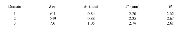
In figure 3, the time and spanwise-averaged velocity profiles at the centre location of each measurement are compared with the Blasius profile (White & Majdalani Reference White and Majdalani2006). The local boundary layer displacement thickness was determined and employed to non-dimensionalise the wall-normal distance; velocities were scaled on the free stream velocity
 $U_\infty$
. The velocity profiles measured by Tomo-PIV exhibit a good agreement with the Blasius profile. The boundary layer parameters of these velocity profiles are summarised in table 2, demonstrating that the initial boundary layer in the present experiment is a typical Blasius laminar boundary layer. The time resolution is
$U_\infty$
. The velocity profiles measured by Tomo-PIV exhibit a good agreement with the Blasius profile. The boundary layer parameters of these velocity profiles are summarised in table 2, demonstrating that the initial boundary layer in the present experiment is a typical Blasius laminar boundary layer. The time resolution is
 $\Delta t=0.002$
s for all cases and the spatial resolution for each region is presented in table 1. Using perspective calibration and volume self-calibration operations, the calibration error was reduced to less than 0.1 pixels. The signal-to-noise ratio (SNR) measures the quality of the reconstructed volume, calculated by comparing the intensity of the illuminated volume to the intensity outside of it. The SNR of each measurement domain is presented in table 1. All measurements have an SNR larger than 2, which indicates a high-quality reconstruction (Scarano Reference Scarano2013).
$\Delta t=0.002$
s for all cases and the spatial resolution for each region is presented in table 1. Using perspective calibration and volume self-calibration operations, the calibration error was reduced to less than 0.1 pixels. The signal-to-noise ratio (SNR) measures the quality of the reconstructed volume, calculated by comparing the intensity of the illuminated volume to the intensity outside of it. The SNR of each measurement domain is presented in table 1. All measurements have an SNR larger than 2, which indicates a high-quality reconstruction (Scarano Reference Scarano2013).
Table 2. Boundary layer characteristics:
 $\textrm {Re}_{\delta ^*}$
is the Reynolds number based on local displacement thickness;
$\textrm {Re}_{\delta ^*}$
is the Reynolds number based on local displacement thickness;
 $\delta _{\theta }$
is the momentum thickness;
$\delta _{\theta }$
is the momentum thickness;
 $\delta ^*$
is the displacement thickness;
$\delta ^*$
is the displacement thickness;
 $H$
is the shape factor.
$H$
is the shape factor.
2.2. Numerical method
2.2.1. DNS set-up
DNS was performed using an open-source pseudo-spectral solver Simson (Chevalier et al. Reference Chevalier, Schlatter, Lundbladh and Henningson2007), which has been employed by many previous boundary layer simulation investigations (Brandt & Henningson Reference Brandt and Henningson2002; Brandt et al. Reference Brandt, Schlatter and Henningson2004). The incompressible Navier–Stokes equations were solved to obtain a data set for turbulent spots developing within a zero pressure gradient flat plate boundary layer.
The spatial discretisation in the streamwise and spanwise directions employs Fourier series expansions. Chebyshev polynomial series are used in wall-normal direction discretisation. For time discretisation, a second-order Crank–Nicolson method is used to handle the linear term, while a third-order four-stage Runge–Kutta method is employed for the nonlinear components. The coordinate system is defined to match that used in the experiment, allowing comparison between the simulation and experimental results.

Figure 4. Schematic diagram of the computational domain.
As illustrated in figure 4, the computational domain dimensions in the streamwise, wall-normal and spanwise directions are
 $400\delta ^*_0$
,
$400\delta ^*_0$
,
 $25\delta ^*_0$
and
$25\delta ^*_0$
and
 $90\delta ^*_0$
, respectively, where
$90\delta ^*_0$
, respectively, where
 $\delta ^*_0$
is the displacement thickness at the inlet of the computational domain. Grid resolution was selected based on studies (Levin & Henningson Reference Levin and Henningson2007) at comparable Reynolds numbers. Verification was conducted on three different grid densities: Grid 1 (800, 181 and 360 nodes in the streamwise, spanwise and wall-normal directions, respectively); Grid 2 (1600, 241 and 480 nodes); and Grid 3 (2000, 301 and 600 nodes). A comparison of structures within the young turbulent spot showed no observable differences between Grids 2 and 3. Consequently, Grid 2 was employed for this numerical simulation, featuring uniformly distributed nodes in the
$\delta ^*_0$
is the displacement thickness at the inlet of the computational domain. Grid resolution was selected based on studies (Levin & Henningson Reference Levin and Henningson2007) at comparable Reynolds numbers. Verification was conducted on three different grid densities: Grid 1 (800, 181 and 360 nodes in the streamwise, spanwise and wall-normal directions, respectively); Grid 2 (1600, 241 and 480 nodes); and Grid 3 (2000, 301 and 600 nodes). A comparison of structures within the young turbulent spot showed no observable differences between Grids 2 and 3. Consequently, Grid 2 was employed for this numerical simulation, featuring uniformly distributed nodes in the
 $x$
and
$x$
and
 $z$
directions, with a mesh refinement near the wall in the
$z$
directions, with a mesh refinement near the wall in the
 $y$
direction.
$y$
direction.
Periodic boundary conditions are applied in all horizontal directions. To achieve spatial simulation, an additional fringe region of length 100
 $\delta ^*_0$
is added following the physical domain to dampen disturbances and ensure that the flow returns to the inlet condition. A no-slip boundary condition is specified at the wall surface. The upper surface of the computational domain is a uniform free stream boundary condition.
$\delta ^*_0$
is added following the physical domain to dampen disturbances and ensure that the flow returns to the inlet condition. A no-slip boundary condition is specified at the wall surface. The upper surface of the computational domain is a uniform free stream boundary condition.
In the present simulation, the Reynolds number is expressed as
 $Re=U_0\delta ^*/\nu$
, where
$Re=U_0\delta ^*/\nu$
, where
 $\delta ^*$
is the displacement thickness at the local position and
$\delta ^*$
is the displacement thickness at the local position and
 $\nu$
is the kinematic viscosity. The Reynolds number at the inlet of the domain is prescribed as 490. The displacement thickness
$\nu$
is the kinematic viscosity. The Reynolds number at the inlet of the domain is prescribed as 490. The displacement thickness
 $\delta ^*_0$
at the inlet is used to scale the length in the present simulation. Here,
$\delta ^*_0$
at the inlet is used to scale the length in the present simulation. Here,
 $U_0$
is the reference velocity, where
$U_0$
is the reference velocity, where
 $U_0$
is free stream velocity. The reference time is
$U_0$
is free stream velocity. The reference time is
 $\delta ^*_0/U_0$
. Turbulent spots are initialised by localised blowing of duration
$\delta ^*_0/U_0$
. Turbulent spots are initialised by localised blowing of duration
 $t=3$
, where
$t=3$
, where
 $t$
is the dimensionless time. The blowing location is 59
$t$
is the dimensionless time. The blowing location is 59
 $\delta ^*_0$
downstream from the inlet. The Reynolds number is 571 at the blowing location, which is greater than the flat plate boundary layer critical Reynolds number of
$\delta ^*_0$
downstream from the inlet. The Reynolds number is 571 at the blowing location, which is greater than the flat plate boundary layer critical Reynolds number of
 $ {Re}_{crit}=520$
(Schlichting & Gersten Reference Schlichting and Gersten2016). The dimensions of the blowing disturbance in the
$ {Re}_{crit}=520$
(Schlichting & Gersten Reference Schlichting and Gersten2016). The dimensions of the blowing disturbance in the
 $x$
and
$x$
and
 $z$
directions are 2.4
$z$
directions are 2.4
 $\delta ^*_0$
and 2
$\delta ^*_0$
and 2
 $\delta ^*_0$
, respectively. The spatial and temporal distribution of the perturbation is given by
$\delta ^*_0$
, respectively. The spatial and temporal distribution of the perturbation is given by
 \begin{equation} v_{wall}=A_0f(x)f(z)f(t), \end{equation}
where the function
 $f$
is defined as
$f$
is defined as
 \begin{equation} f(x)=S\left (\frac {x-x_{start}}{\varDelta _{rise}}\right )-S\left (\frac {x-x_{end}}{\varDelta _{fall}}+1\right ), \end{equation}
 \begin{equation} S(x) = \left \{ \begin{array}{ll} 0, & x\leqslant 0, \\[6pt] 1/\left [1+\exp ({1/(x-1)+1/x})\right ], & 0\lt x\lt 1, \\[6pt] 1, & x\geqslant 1. \end{array} \right . \end{equation}
Here,
 $v_{wall}$
is the wall-normal velocity at the wall surface;
$v_{wall}$
is the wall-normal velocity at the wall surface;
 $\varDelta _{rise}$
and
$\varDelta _{rise}$
and
 $\varDelta _{fall}$
are the rise and fall distance of the function
$\varDelta _{fall}$
are the rise and fall distance of the function
 $f(x)$
. The amplitude
$f(x)$
. The amplitude
 $A_0$
is set to 0.8, which was determined to be sufficient to trigger a turbulent spot.
$A_0$
is set to 0.8, which was determined to be sufficient to trigger a turbulent spot.
2.3. Lagrangian tracking approach
The 3-D velocity fields obtained from Tomo-PIV measurements and DNS are used for Lagrangian tracking of specific particles, enabling the observation of flow patterns created by a turbulent spot. Streaklines are constructed by connecting multiple particles initiated at different times, from a fixed position. Timelines are obtained by simultaneously tracking multiple particles initiated at different initial positions but at the same initial time. Tracking a group of particles comprising an initially flat surface allows the behaviour and evolution of an initially flat material surface to be assessed. The trajectory of a particle in a fluid medium is determined by numerically integrating the following ordinary differential equation (ODE):
 \begin{equation} \overrightarrow {V}(\overrightarrow {X}(t),t)= {\rm d}\overrightarrow {X}(t)/{\rm d}t. \end{equation}
The instantaneous velocity,
 $V(X,t)$
, is derived from the datasets obtained from the Tomo-PIV experiments or DNS. The integration time step,
$V(X,t)$
, is derived from the datasets obtained from the Tomo-PIV experiments or DNS. The integration time step,
 ${\rm d}t$
, is used to calculate the displacement vector,
${\rm d}t$
, is used to calculate the displacement vector,
 ${\rm d}X(t)$
, for each integration step. The integration time step (
${\rm d}X(t)$
, for each integration step. The integration time step (
 ${\rm d}t$
) for the experimental tracking is 0.002 s, consistent with the time resolution of the Tomo-PIV. The integration time step (
${\rm d}t$
) for the experimental tracking is 0.002 s, consistent with the time resolution of the Tomo-PIV. The integration time step (
 ${\rm d}t$
) for the DNS tracking is one dimensionless time unit. The integration process is conducted from the initial time,
${\rm d}t$
) for the DNS tracking is one dimensionless time unit. The integration process is conducted from the initial time,
 $t_0$
, to the final time,
$t_0$
, to the final time,
 $t_1$
, with an initial condition of
$t_1$
, with an initial condition of
 $X_0$
. A MATLAB algorithm using the Dormand–Prince method is employed to numerically solve (2.4), with absolute and relative tolerances of the ODE solver set at
$X_0$
. A MATLAB algorithm using the Dormand–Prince method is employed to numerically solve (2.4), with absolute and relative tolerances of the ODE solver set at
 $10^{-6}$
. The present study employs the Lagrangian tracking methods developed by Jiang et al. (Reference Jiang, Lee, Chen, Smith and Linden2020a
,Reference Jiang, Lee, Smith, Chen and Linden
b
, Reference Jiang, Gu, Lee, Smith and Linden2021), which have been used effectively for transitional and turbulent boundary layers.
$10^{-6}$
. The present study employs the Lagrangian tracking methods developed by Jiang et al. (Reference Jiang, Lee, Chen, Smith and Linden2020a
,Reference Jiang, Lee, Smith, Chen and Linden
b
, Reference Jiang, Gu, Lee, Smith and Linden2021), which have been used effectively for transitional and turbulent boundary layers.
3. Experiment results
The detailed experimental conditions were described in § 2.1. Three Tomo-PIV measurement domains cover the region from the initiation of a turbulent spot to a fully developed turbulent spot. By analysing the characteristic patterns within the three domains, the main flow characteristics and potential flow structures of the turbulent spot evolution process have been identified. The local coordinate systems of the three domains used in the Tomo-PIV measurements are transformed into the coordinates system defined in § 2.1.1, thereby allowing the determination of the relative location for the three domains.

Figure 5. Evolution of the streamwise fluctuating velocity of turbulent spots in the
 $y$
–
$y$
–
 $t$
plane: (
$t$
plane: (
 $a$
)
$a$
)
 $x/\delta ^\ast_0=25$
in Domain 1; (
$x/\delta ^\ast_0=25$
in Domain 1; (
 $b$
)
$b$
)
 $x/\delta ^\ast_0=45$
in Domain 1; (
$x/\delta ^\ast_0=45$
in Domain 1; (
 $c$
)
$c$
)
 $x/\delta ^\ast_0=55$
in Domain 2; (
$x/\delta ^\ast_0=55$
in Domain 2; (
 $d$
)
$d$
)
 $x/\delta ^\ast_0=75$
in Domain 2; (
$x/\delta ^\ast_0=75$
in Domain 2; (
 $e$
)
$e$
)
 $x/\delta ^\ast_0=115$
in Domain 3; (
$x/\delta ^\ast_0=115$
in Domain 3; (
 $f$
)
$f$
)
 $x/\delta ^\ast_0=135$
in Domain 3.
$x/\delta ^\ast_0=135$
in Domain 3.
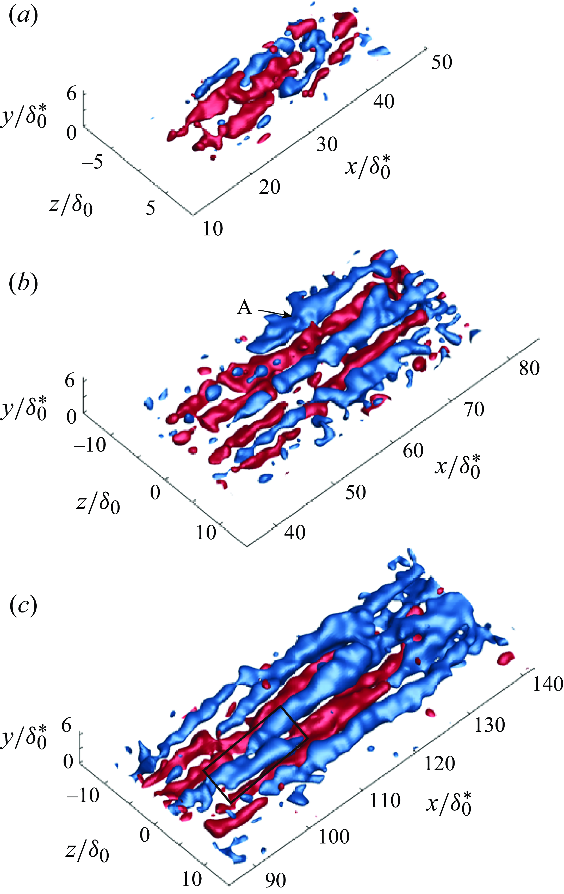
Figure 6. Evolution of the isosurfaces of streamwise fluctuating velocity in the experiment: (
 $a$
) Domain 1; (
$a$
) Domain 1; (
 $b$
) Domain 2; (
$b$
) Domain 2; (
 $c$
) Domain 3. The blue and red isosurfaces correspond to the negative and positive streamwise fluctuating velocities, respectively. The isosurfaces in panel (
$c$
) Domain 3. The blue and red isosurfaces correspond to the negative and positive streamwise fluctuating velocities, respectively. The isosurfaces in panel (
 $a{-}c$
) correspond to
$a{-}c$
) correspond to
 $u'/U_{\infty } = \pm 6.5\, \%$
. There is no time correlation among panels (
$u'/U_{\infty } = \pm 6.5\, \%$
. There is no time correlation among panels (
 $a$
), (
$a$
), (
 $b$
) and (
$b$
) and (
 $c$
).
$c$
).
The fluctuating velocity field in the experiment was determined by subtracting the time-average undisturbed laminar boundary layer velocity field from the instantaneous velocity field. Figure 5 shows the spatial/temporal behaviour of the streamwise fluctuating velocity on the central plane of a turbulent spot in
 $y$
–
$y$
–
 $t$
coordinates. In Domain 1, the low-speed fluid ejected by the wall-normal jet quickly moves outside the boundary layer. The disturbance can be still detected at approximately
$t$
coordinates. In Domain 1, the low-speed fluid ejected by the wall-normal jet quickly moves outside the boundary layer. The disturbance can be still detected at approximately
 $y/\delta ^\ast_0=6.5$
. In Domain 2, the low-speed region expands in the streamwise direction and moves further away from the wall, with the highest detectable disturbance position at approximately
$y/\delta ^\ast_0=6.5$
. In Domain 2, the low-speed region expands in the streamwise direction and moves further away from the wall, with the highest detectable disturbance position at approximately
 $y/\delta ^\ast_0=6.8$
. In Domain 3, the low-speed region at the centre of the turbulent spot rises further, reaching a height of approximately
$y/\delta ^\ast_0=6.8$
. In Domain 3, the low-speed region at the centre of the turbulent spot rises further, reaching a height of approximately
 $y/\delta ^\ast_0=7$
. As the initial disturbance advects downstream, both the dimensions and intensity of the low-speed regions increase, with these low-speed regions progressively moving away from the wall and high-speed regions developing near the wall. The patterns of the streamwise fluctuating velocity shown in figure 5 agree well with previous observations of turbulent spots (Wygnanski et al. Reference Wygnanski, Zilberman and Haritonidis1982; Wang et al. Reference Wang, Choi, Gaster, Atkin, Borodulin and Kachanov2021).
$y/\delta ^\ast_0=7$
. As the initial disturbance advects downstream, both the dimensions and intensity of the low-speed regions increase, with these low-speed regions progressively moving away from the wall and high-speed regions developing near the wall. The patterns of the streamwise fluctuating velocity shown in figure 5 agree well with previous observations of turbulent spots (Wygnanski et al. Reference Wygnanski, Zilberman and Haritonidis1982; Wang et al. Reference Wang, Choi, Gaster, Atkin, Borodulin and Kachanov2021).
To further illustrate the development of high- and low-speed streaks within the turbulent spot, figure 6 displays isosurfaces of streamwise fluctuating velocity for the three measurement domains. As shown in figure 6, the high- (red) and low-speed (blue) regions within the turbulent spot are arranged in somewhat alternating patterns. In figure 6(
 $a$
) (Domain 1), the high- and low-speed regions appear shorter and less organised. As the low-speed regions travel downstream, they become more organised, and grow in both streamwise and spanwise directions. By comparison with the structures observed in Domain 1, figure 6(
$a$
) (Domain 1), the high- and low-speed regions appear shorter and less organised. As the low-speed regions travel downstream, they become more organised, and grow in both streamwise and spanwise directions. By comparison with the structures observed in Domain 1, figure 6(
 $b$
) (Domain 2) shows the development of two low-speed regions at approximately
$b$
) (Domain 2) shows the development of two low-speed regions at approximately
 $z/\delta ^\ast_0=\pm 7$
. Figure 6(
$z/\delta ^\ast_0=\pm 7$
. Figure 6(
 $c$
) shows that by Domain 3, the low-speed regions further increase in breadth and length, and additional low-speed regions begin to develop near the trailing sides of the turbulent spot. The results indicate that as the turbulent spot advances downstream, low-speed regions appear at the turbulent spot edges, contributing to the expansion of the turbulent spot. Moreover, the low-speed region that appears within the rectangular box indicated in figure 6(
$c$
) shows that by Domain 3, the low-speed regions further increase in breadth and length, and additional low-speed regions begin to develop near the trailing sides of the turbulent spot. The results indicate that as the turbulent spot advances downstream, low-speed regions appear at the turbulent spot edges, contributing to the expansion of the turbulent spot. Moreover, the low-speed region that appears within the rectangular box indicated in figure 6(
 $c$
) appears to result from the merging of two low-speed regions. This phenomenon will be further investigated in subsequent sections. Similar observations of low-speed streak amalgamation have been reported by Wang et al. (Reference Wang, Choi, Gaster, Atkin, Borodulin and Kachanov2021). Figure 6 suggests that the development of low-speed streaks at the periphery of the turbulent spot is closely associated with the growth of turbulent spots.
$c$
) appears to result from the merging of two low-speed regions. This phenomenon will be further investigated in subsequent sections. Similar observations of low-speed streak amalgamation have been reported by Wang et al. (Reference Wang, Choi, Gaster, Atkin, Borodulin and Kachanov2021). Figure 6 suggests that the development of low-speed streaks at the periphery of the turbulent spot is closely associated with the growth of turbulent spots.

Figure 7. Timeline patterns in measurement Domain 1 initiated at
 $x/\delta ^\ast_0 =20.7$
and
$x/\delta ^\ast_0 =20.7$
and
 $y/\delta ^\ast_0=1.43$
: (
$y/\delta ^\ast_0=1.43$
: (
 $a$
) timeline pattern at
$a$
) timeline pattern at
 $t=49.4$
; (
$t=49.4$
; (
 $b$
) timeline pattern at
$b$
) timeline pattern at
 $t=61.7$
.
$t=61.7$
.

Figure 8. Timeline patterns in measurement Domain 2 initiated at
 $x/\delta ^\ast_0 =48.5$
and
$x/\delta ^\ast_0 =48.5$
and
 $y/\delta ^\ast_0=1.37$
: (
$y/\delta ^\ast_0=1.37$
: (
 $a$
) timeline pattern at
$a$
) timeline pattern at
 $t=68$
; (
$t=68$
; (
 $b$
) timeline pattern at
$b$
) timeline pattern at
 $t=77$
.
$t=77$
.
The timelines reconstructed from the 3-D velocity field are similar to the hydrogen bubble visualisation. In previous studies, Jiang et al. (Reference Jiang, Lee, Chen, Smith and Linden2020a
,Reference Jiang, Lee, Smith, Chen and Linden
b
) used timelines to visualise the low-speed streaks in transitional and turbulent boundary layers. Here, timelines are used to visualise the flow patterns created by turbulent spots. The colour of the timelines represents their distance from the wall. Their spanwise profiles are indicative of the streamwsie velocity in the corresponding region, which shows the high- and low-speed regions within turbulent spots. The timeline patterns of the turbulent spot for Domains 1 and 2 are illustrated in figures 7 and 8, respectively. In figure 7, spanwise timelines are initiated at
 $x/\delta ^\ast_0 =20.7$
,
$x/\delta ^\ast_0 =20.7$
,
 $y/\delta ^\ast_0 =1.43$
in Domain 1 to show the initial structure downstream of the jet orifice. In figure 7(
$y/\delta ^\ast_0 =1.43$
in Domain 1 to show the initial structure downstream of the jet orifice. In figure 7(
 $a$
), an uplifted
$a$
), an uplifted
 $\Lambda$
-shaped region labelled as A is discernible. Subsequently, figure 7(
$\Lambda$
-shaped region labelled as A is discernible. Subsequently, figure 7(
 $b$
) shows an
$b$
) shows an
 $\Lambda$
-shaped vortex, characterised by the intertwining of timelines labelled as A. Furthermore, the intertwining observed in the timelines labelled B suggests the formation of vortices on the inner side of structure A.
$\Lambda$
-shaped vortex, characterised by the intertwining of timelines labelled as A. Furthermore, the intertwining observed in the timelines labelled B suggests the formation of vortices on the inner side of structure A.
To show the timeline patterns created by the turbulent spot in Domain 2, in figure 8, spanwise timelines are initiated at
 $x/\delta ^\ast_0 =48.5$
and
$x/\delta ^\ast_0 =48.5$
and
 $y/\delta ^\ast_0 =1.37$
. In figure 8, the dashed lines S1 and S2 roughly indicate two low-speed streaks, which correspond to the low-speed streaks at
$y/\delta ^\ast_0 =1.37$
. In figure 8, the dashed lines S1 and S2 roughly indicate two low-speed streaks, which correspond to the low-speed streaks at
 $z/\delta ^\ast_0=\pm 7$
on the lateral edges of the turbulent spot shown in figure 6(
$z/\delta ^\ast_0=\pm 7$
on the lateral edges of the turbulent spot shown in figure 6(
 $b$
). The low-speed region S1 in figure 8 approximately spans
$b$
). The low-speed region S1 in figure 8 approximately spans
 $z/\delta ^\ast_0 =-8$
to
$z/\delta ^\ast_0 =-8$
to
 $-5$
. Additionally, an adjacent high-speed region is observed spanning
$-5$
. Additionally, an adjacent high-speed region is observed spanning
 $z/\delta ^\ast_0 =-5$
to
$z/\delta ^\ast_0 =-5$
to
 $-2.5$
. The low-speed region S2 approximately spans
$-2.5$
. The low-speed region S2 approximately spans
 $z/\delta ^\ast_0 =4.7$
to 7.7, with an adjacent high-speed region located between
$z/\delta ^\ast_0 =4.7$
to 7.7, with an adjacent high-speed region located between
 $z/\delta ^\ast_0 =2.1$
and 4.7. In figure 8(
$z/\delta ^\ast_0 =2.1$
and 4.7. In figure 8(
 $a$
), the timelines near
$a$
), the timelines near
 $z/\delta ^\ast_0=\pm 7$
do not exhibit significant intertwining or rotational behaviour, suggesting that these two low-speed streaks are not the result of vortex interactions. Figure 8(
$z/\delta ^\ast_0=\pm 7$
do not exhibit significant intertwining or rotational behaviour, suggesting that these two low-speed streaks are not the result of vortex interactions. Figure 8(
 $b$
) shows that the timelines within the regions of the two low-speed streaks, S1 and S2, begin to concentrate at the interface between the low-speed and high-speed regions, indicating the development of high-shear layers.
$b$
) shows that the timelines within the regions of the two low-speed streaks, S1 and S2, begin to concentrate at the interface between the low-speed and high-speed regions, indicating the development of high-shear layers.

Figure 9. Evolution of spanwise timelines initiated at
 $x/\delta ^\ast_0=41$
,
$x/\delta ^\ast_0=41$
,
 $y/\delta ^\ast_0=1.1$
and
$y/\delta ^\ast_0=1.1$
and
 $t=24.7$
showing the low-speed streak labelled A in figure 6(
$t=24.7$
showing the low-speed streak labelled A in figure 6(
 $b$
): (
$b$
): (
 $a$
)
$a$
)
 $t=30.9$
; (
$t=30.9$
; (
 $b$
)
$b$
)
 $t=38.6$
; (
$t=38.6$
; (
 $c$
)
$c$
)
 $t=46.3$
; (
$t=46.3$
; (
 $d$
)
$d$
)
 $t=54.0$
. The sequence of red dots corresponds to a streakline initiated at
$t=54.0$
. The sequence of red dots corresponds to a streakline initiated at
 $z/\delta ^\ast_0=7$
.
$z/\delta ^\ast_0=7$
.

Figure 10. Vorticity colour maps in the
 $x$
–
$x$
–
 $z$
plane at
$z$
plane at
 $y/\delta ^\ast_0=1.1$
and
$y/\delta ^\ast_0=1.1$
and
 $t=54$
: (
$t=54$
: (
 $a$
) wall-normal vorticity
$a$
) wall-normal vorticity
 $\omega _y$
; (
$\omega _y$
; (
 $b$
) streamwise vorticity
$b$
) streamwise vorticity
 $\omega _x$
.
$\omega _x$
.
To illustrate the temporal evolution of the low-speed streaks at the lateral edge of the turbulent spot in Domain 2, the low-speed region labelled A in figure 6 (
 $b$
) is more closely examined in figure 9. The timelines are initiated at
$b$
) is more closely examined in figure 9. The timelines are initiated at
 $x/\delta ^\ast_0=41$
and
$x/\delta ^\ast_0=41$
and
 $y/\delta ^\ast_0=1.37$
. The red dotted lines in figure 9 show a streakline initiated at
$y/\delta ^\ast_0=1.37$
. The red dotted lines in figure 9 show a streakline initiated at
 $z/\delta ^\ast_0=7$
. The low-speed region A is approximately located between
$z/\delta ^\ast_0=7$
. The low-speed region A is approximately located between
 $z/\delta ^\ast_0=-8$
and
$z/\delta ^\ast_0=-8$
and
 $-5$
, flanked by high-speed regions on either side. The sequence of timeline patterns in figure 9 illustrates that an accumulation of timelines mainly occurs at the interface between high- and low-speed regions, indicating the presence of strong shear at the boundary between these regions.
$-5$
, flanked by high-speed regions on either side. The sequence of timeline patterns in figure 9 illustrates that an accumulation of timelines mainly occurs at the interface between high- and low-speed regions, indicating the presence of strong shear at the boundary between these regions.
Figure 10 shows the wall-normal and streamwise vorticity contours on the
 $y/\delta ^\ast_0=1.1$
plane for the region corresponding to figure 9 at
$y/\delta ^\ast_0=1.1$
plane for the region corresponding to figure 9 at
 $t=54$
. As shown in figure 10(
$t=54$
. As shown in figure 10(
 $a$
), the positive wall-normal voricity between
$a$
), the positive wall-normal voricity between
 $x/\delta ^\ast_0=45$
and 55 primarily concentrates around
$x/\delta ^\ast_0=45$
and 55 primarily concentrates around
 $z/\delta ^\ast_0=-5$
. In the range of
$z/\delta ^\ast_0=-5$
. In the range of
 $x/\delta ^\ast_0=40{-}45$
, the positive wall-normal vorticity is inclined in the streamwise direction, indicating a streamwise inclination of the boundary between the low-speed region and the high-speed region in this area. The negative wall-normal vorticity related to the low-speed region concentrates around
$x/\delta ^\ast_0=40{-}45$
, the positive wall-normal vorticity is inclined in the streamwise direction, indicating a streamwise inclination of the boundary between the low-speed region and the high-speed region in this area. The negative wall-normal vorticity related to the low-speed region concentrates around
 $z/\delta ^\ast_0=-8$
, but its intensity is weaker than that of the positive wall-normal vorticity. Figure 10(
$z/\delta ^\ast_0=-8$
, but its intensity is weaker than that of the positive wall-normal vorticity. Figure 10(
 $b$
) shows that the positive streamwise vorticity primarily concentrates in the region of
$b$
) shows that the positive streamwise vorticity primarily concentrates in the region of
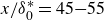 $x/\delta ^\ast_0=45{-}55$
near
$x/\delta ^\ast_0=45{-}55$
near
 $z/\delta ^\ast_0=-5$
, while the development of negative streamwise vorticity is relatively weak. Cumulatively, figures 9(
$z/\delta ^\ast_0=-5$
, while the development of negative streamwise vorticity is relatively weak. Cumulatively, figures 9(
 $d$
) and 10 show that vorticity primarily concentrates along the boundary between the high-speed and low-speed regions. The streamwise and spanwise vorticity on the
$d$
) and 10 show that vorticity primarily concentrates along the boundary between the high-speed and low-speed regions. The streamwise and spanwise vorticity on the
 $z/\delta ^\ast_0=-5$
side is stronger because the high-speed region around
$z/\delta ^\ast_0=-5$
side is stronger because the high-speed region around
 $z/\delta ^\ast_0=-5$
exhibits a higher streamwise velocity compared with the high-speed region near
$z/\delta ^\ast_0=-5$
exhibits a higher streamwise velocity compared with the high-speed region near
 $z/\delta ^\ast_0=-8$
.
$z/\delta ^\ast_0=-8$
.

Figure 11. Behaviour of a material surface initiated at
 $y/\delta ^\ast_0=1.1$
illustrating the effects of the low-speed streak labelled A in figure 6(
$y/\delta ^\ast_0=1.1$
illustrating the effects of the low-speed streak labelled A in figure 6(
 $b$
): (
$b$
): (
 $a$
)
$a$
)
 $t=30.9$
; (
$t=30.9$
; (
 $b$
)
$b$
)
 $t=38.6$
; (
$t=38.6$
; (
 $c$
)
$c$
)
 $t=46.3$
; (
$t=46.3$
; (
 $d$
)
$d$
)
 $t=54.0$
.
$t=54.0$
.
To illustrate the spatio-temporal evolution of the low-speed streak labelled A in figure 6(b), a material surface was initiated at
 $y/\delta ^\ast_0=1.1$
and
$y/\delta ^\ast_0=1.1$
and
 $t=30.9$
, within the low-speed streak region. Figure 11 shows the sequential deformation undergone by the material surface. Figure 11(
$t=30.9$
, within the low-speed streak region. Figure 11 shows the sequential deformation undergone by the material surface. Figure 11(
 $b$
) shows that the central portion of the material surface begins to lift up. Meanwhile, the spanwise edge of the material surface undergoes a downward movement, which illustrates that the surrounding fluid moves towards the wall. Figure 11(
$b$
) shows that the central portion of the material surface begins to lift up. Meanwhile, the spanwise edge of the material surface undergoes a downward movement, which illustrates that the surrounding fluid moves towards the wall. Figure 11(
 $c$
) shows bulges labelled A and B developing on the material sheet. Figure 11(
$c$
) shows bulges labelled A and B developing on the material sheet. Figure 11(
 $d$
) shows that as these bulges continue to develop, the central portion of the material surface develops into a lifted streaky region. The deformation of the material surface observed in figure 11 closely resembles the deformation of material surfaces (see figure 1
$d$
) shows that as these bulges continue to develop, the central portion of the material surface develops into a lifted streaky region. The deformation of the material surface observed in figure 11 closely resembles the deformation of material surfaces (see figure 1
 $a$
) observed by Jiang et al. (Reference Jiang, Lee, Chen, Smith and Linden2020a
) during the later stages of transition flows. The behaviour of the material surface shown in figure 11 suggests that the lift-up of the local low-speed streak behaves as 3-D waves.
$a$
) observed by Jiang et al. (Reference Jiang, Lee, Chen, Smith and Linden2020a
) during the later stages of transition flows. The behaviour of the material surface shown in figure 11 suggests that the lift-up of the local low-speed streak behaves as 3-D waves.

Figure 12. Spanwise timelines showing the low-speed streaks within the turbulent spot in Domain 3. (a,b) Spanwise timelines initiated at
 $x/\delta ^\ast_0=106.3$
,
$x/\delta ^\ast_0=106.3$
,
 $y/\delta ^\ast_0=1.6$
and
$y/\delta ^\ast_0=1.6$
and
 $t =74.1$
. (c,d) Spanwise timelines initiated at
$t =74.1$
. (c,d) Spanwise timelines initiated at
 $x/\delta ^\ast_0=122.1$
,
$x/\delta ^\ast_0=122.1$
,
 $y/\delta ^\ast_0=1.6$
and
$y/\delta ^\ast_0=1.6$
and
 $t =95.7$
. The sequences of the red particles are streaklines initiated at
$t =95.7$
. The sequences of the red particles are streaklines initiated at
 $z/\delta ^\ast_0=0.4$
, 3.2, and 7.9: (
$z/\delta ^\ast_0=0.4$
, 3.2, and 7.9: (
 $a$
)
$a$
)
 $t=92.6$
; (
$t=92.6$
; (
 $b$
)
$b$
)
 $t=95.7$
; (
$t=95.7$
; (
 $c$
)
$c$
)
 $t=114.2$
; (
$t=114.2$
; (
 $d$
)
$d$
)
 $t=117.3$
.
$t=117.3$
.

Figure 13. Deformation of a material surface initiated at
 $t=86.4$
, at
$t=86.4$
, at
 $y/\delta ^\ast_0=1.4$
, reflecting subsequent behaviour of the low-speed streaks shown in figure 12: (
$y/\delta ^\ast_0=1.4$
, reflecting subsequent behaviour of the low-speed streaks shown in figure 12: (
 $a$
)
$a$
)
 $t=92.6$
; (
$t=92.6$
; (
 $b$
)
$b$
)
 $t=95.7$
; (
$t=95.7$
; (
 $c$
)
$c$
)
 $t=98.8$
; (
$t=98.8$
; (
 $d$
)
$d$
)
 $t=101.9$
.
$t=101.9$
.
In figure 6(
 $c$
) (Domain 3), the amalgamation between low-speed streaks was identified using a rectangular box in the figure. To investigate this amalgamation process, the data set obtained from measurement Domain 3 was further analysed. Spanwise timelines were initiated in the region of Domain 3 where amalgamation of the low-speed streaks takes place. The timelines are initiated at a frequency of 500 Hz. Figures 12(
$c$
) (Domain 3), the amalgamation between low-speed streaks was identified using a rectangular box in the figure. To investigate this amalgamation process, the data set obtained from measurement Domain 3 was further analysed. Spanwise timelines were initiated in the region of Domain 3 where amalgamation of the low-speed streaks takes place. The timelines are initiated at a frequency of 500 Hz. Figures 12(
 $a$
) and 12(
$a$
) and 12(
 $b$
) illustrate the presence of three low-speed streaks at
$b$
) illustrate the presence of three low-speed streaks at
 $t=92.6$
and 95.7 within this region. The sequences of red particles in figures 12(
$t=92.6$
and 95.7 within this region. The sequences of red particles in figures 12(
 $a$
) and 12(
$a$
) and 12(
 $b$
) are streaklines, roughly indicating the locations of the three low-speed streaks. The three low-speed streaks are identified as I, II and III from top to bottom. Note that the spacing between low-speed streaks I and II is smaller than the spacing between streaks II and III, indicating a higher likelihood of amalgamation between low-speed streaks I and II. In figures 12(
$b$
) are streaklines, roughly indicating the locations of the three low-speed streaks. The three low-speed streaks are identified as I, II and III from top to bottom. Note that the spacing between low-speed streaks I and II is smaller than the spacing between streaks II and III, indicating a higher likelihood of amalgamation between low-speed streaks I and II. In figures 12(
 $a$
) and 12(
$a$
) and 12(
 $b$
), A high-speed streak is clearly observed at approximately
$b$
), A high-speed streak is clearly observed at approximately
 $z/\delta ^\ast_0=2$
between low-speed streaks I and II. Figures 12(
$z/\delta ^\ast_0=2$
between low-speed streaks I and II. Figures 12(
 $c$
) and 12(
$c$
) and 12(
 $d$
) show the timelines initiated at a further downstream location
$d$
) show the timelines initiated at a further downstream location
 $x/\delta ^\ast_0=122.1$
. The high-speed streak observed at approximately
$x/\delta ^\ast_0=122.1$
. The high-speed streak observed at approximately
 $z/\delta ^\ast_0=2$
in figures 12(
$z/\delta ^\ast_0=2$
in figures 12(
 $a$
) and 12(
$a$
) and 12(
 $b$
) is almost not visible in the timelines shown in figures 12(
$b$
) is almost not visible in the timelines shown in figures 12(
 $c$
) and 12(
$c$
) and 12(
 $d$
), which means that the boundary between low-speed streaks I and II has become indistinct, and that low-speed streaks I and II are undergoing an amalgamation.
$d$
), which means that the boundary between low-speed streaks I and II has become indistinct, and that low-speed streaks I and II are undergoing an amalgamation.
To further illustrate the behaviour and effects of low-speed streaks I, II and III, a localised material surface is initiated at
 $y/\delta ^\ast_0=1.4$
and
$y/\delta ^\ast_0=1.4$
and
 $t=86.4$
in the region spanning
$t=86.4$
in the region spanning
 $2\lt z/\delta ^\ast_0\lt 9$
by
$2\lt z/\delta ^\ast_0\lt 9$
by
 $105\lt x/\delta ^\ast_0\lt 114$
. Figure 13 shows the subsequent spatial-temporal evolution of the material surface. Figure 13(
$105\lt x/\delta ^\ast_0\lt 114$
. Figure 13 shows the subsequent spatial-temporal evolution of the material surface. Figure 13(
 $a$
) shows that by
$a$
) shows that by
 $t=92.6$
three streamwise lift-up regions develop in the material sheet, which corresponds to the three low-speed streaks identified in figures 12(
$t=92.6$
three streamwise lift-up regions develop in the material sheet, which corresponds to the three low-speed streaks identified in figures 12(
 $a$
) and 12(
$a$
) and 12(
 $b$
). The material surface reveals depressions on both sides of the lift-up regions, indicating a downward motion of higher-speed fluid. The alternating distributions of the uplift and depression of the material surface in the spanwise direction are directly associated with the alternating distribution of high- and low-speed streaks within the turbulent spot. Figure 13 shows that each low-speed streak, as it lifts up from the near-wall region, exhibits a wave-like pattern on the material sheet. The colour contours of the material surface in figure 13(
$b$
). The material surface reveals depressions on both sides of the lift-up regions, indicating a downward motion of higher-speed fluid. The alternating distributions of the uplift and depression of the material surface in the spanwise direction are directly associated with the alternating distribution of high- and low-speed streaks within the turbulent spot. Figure 13 shows that each low-speed streak, as it lifts up from the near-wall region, exhibits a wave-like pattern on the material sheet. The colour contours of the material surface in figure 13(
 $d$
) indicate that the three low-speed streaks exhibit different degrees of lift, suggesting that they are at different stages of development.
$d$
) indicate that the three low-speed streaks exhibit different degrees of lift, suggesting that they are at different stages of development.

Figure 14. The y–z plane cross-sections of material surfaces initiated at a series of heights and
 $t=86.4$
: (
$t=86.4$
: (
 $a$
)
$a$
)
 $x/\delta ^\ast_0=112$
and
$x/\delta ^\ast_0=112$
and
 $t=92.6$
; (
$t=92.6$
; (
 $b$
)
$b$
)
 $x/\delta ^\ast_0=114$
and
$x/\delta ^\ast_0=114$
and
 $t=95.7$
; (
$t=95.7$
; (
 $c$
)
$c$
)
 $x/\delta ^\ast_0=116$
and
$x/\delta ^\ast_0=116$
and
 $t=98.8$
; (
$t=98.8$
; (
 $d$
)
$d$
)
 $x/\delta ^\ast_0=118$
and
$x/\delta ^\ast_0=118$
and
 $t=101.9$
.
$t=101.9$
.

Figure 15. Contours of streamwise fluctuating velocity displaying the amalgamation of the low-speed streaks: (
 $a$
)
$a$
)
 $x/\delta ^\ast_0=112$
and
$x/\delta ^\ast_0=112$
and
 $t=92.6$
; (
$t=92.6$
; (
 $b$
)
$b$
)
 $x/\delta ^\ast_0=114$
and
$x/\delta ^\ast_0=114$
and
 $t=95.7$
; (
$t=95.7$
; (
 $c$
)
$c$
)
 $x/\delta ^\ast_0=116$
and
$x/\delta ^\ast_0=116$
and
 $t=98.8$
; (
$t=98.8$
; (
 $d$
)
$d$
)
 $x/\delta ^\ast_0=118$
and
$x/\delta ^\ast_0=118$
and
 $t=101.9$
.
$t=101.9$
.
Material surfaces at heights ranging from
 $y/\delta ^\ast_0=0.5$
to
$y/\delta ^\ast_0=0.5$
to
 $y/\delta ^\ast_0=4.5$
, initially spaced at intervals of 0.5, were introduced in the same regions as the material surface shown in figure 13. These material surfaces were initiated at
$y/\delta ^\ast_0=4.5$
, initially spaced at intervals of 0.5, were introduced in the same regions as the material surface shown in figure 13. These material surfaces were initiated at
 $t=86.4$
and allowed to develop downstream. In figure 14, cross-sections of these manifold material surfaces at sequential streamwise distances and times illustrate the lift-up process for the three low-speed streaks of figures 12 and 13. Figure 14(
$t=86.4$
and allowed to develop downstream. In figure 14, cross-sections of these manifold material surfaces at sequential streamwise distances and times illustrate the lift-up process for the three low-speed streaks of figures 12 and 13. Figure 14(
 $a$
) identifies three peaks in the material cross-sections, corresponding to the uplift of streaks I, II and III identified in figures 12(
$a$
) identifies three peaks in the material cross-sections, corresponding to the uplift of streaks I, II and III identified in figures 12(
 $a$
) and 12(
$a$
) and 12(
 $b$
). Note that the uplift of streaks I and II is more pronounced compared with streak III. The lowest cross-section displays the peak-valley pattern associated with streak behaviour, suggesting that the uplift of the streaks originates from the near wall. The results shown in figure 14 suggest that the upper material cross-sections are less influenced by the lift-up of the low-speed streaks as compared with the lower cross-sections. Figure 14(
$b$
). Note that the uplift of streaks I and II is more pronounced compared with streak III. The lowest cross-section displays the peak-valley pattern associated with streak behaviour, suggesting that the uplift of the streaks originates from the near wall. The results shown in figure 14 suggest that the upper material cross-sections are less influenced by the lift-up of the low-speed streaks as compared with the lower cross-sections. Figure 14(
 $d$
) shows that the material cross-sections in the vicinity of
$d$
) shows that the material cross-sections in the vicinity of
 $z/\delta ^\ast_0=0$
display a rotational tendency, indicating the development of vortices.
$z/\delta ^\ast_0=0$
display a rotational tendency, indicating the development of vortices.
Figure 15 shows contours of the streamwise fluctuating velocity in the
 $y{-}z$
plane at the streamwise locations and times as shown in figure 14. In figure 15(
$y{-}z$
plane at the streamwise locations and times as shown in figure 14. In figure 15(
 $a$
), three distinct velocity deficit regions are observed in the vicinity of
$a$
), three distinct velocity deficit regions are observed in the vicinity of
 $z/\delta ^\ast_0=0$
, 3 and 7, labelled as A, B and C from left to right, which correspond to the respective low-speed streaks I, II and III. Velocity deficit regions A and B have experienced significant uplift. The downward sweep of high-speed fluid compensates for the low-speed fluid comprising the uplift of streaks I and II, result in positive fluctuating velocity regions near the wall. However, due to the lesser uplift of streak III, no positive fluctuating velocity region is observed beneath deficit region C. In figure 15, there are three velocity excess regions near the wall marked as D, E and F from left to right. Note that the velocity deficit and velocity excess regions display a somewhat alternating pattern. The size and intensity of all velocity deficit regions gradually increase, showing a tendency for amalgamation between adjacent velocity deficit regions. Figures 15(
$z/\delta ^\ast_0=0$
, 3 and 7, labelled as A, B and C from left to right, which correspond to the respective low-speed streaks I, II and III. Velocity deficit regions A and B have experienced significant uplift. The downward sweep of high-speed fluid compensates for the low-speed fluid comprising the uplift of streaks I and II, result in positive fluctuating velocity regions near the wall. However, due to the lesser uplift of streak III, no positive fluctuating velocity region is observed beneath deficit region C. In figure 15, there are three velocity excess regions near the wall marked as D, E and F from left to right. Note that the velocity deficit and velocity excess regions display a somewhat alternating pattern. The size and intensity of all velocity deficit regions gradually increase, showing a tendency for amalgamation between adjacent velocity deficit regions. Figures 15(
 $c$
) and 15(
$c$
) and 15(
 $d$
) show an amalgamation of velocity deficits A and B. At the same time, the intensity of velocity excess region E weakens. Figure 15(
$d$
) show an amalgamation of velocity deficits A and B. At the same time, the intensity of velocity excess region E weakens. Figure 15(
 $d$
) shows the presence of only two velocity deficit regions and two velocity excess regions, while velocity deficit region B and excess region E disappear, apparently having merged with the remaining deficit and excess regions. The merging of velocity deficit regions A and B creates a larger velocity deficit region in the vicinity of
$d$
) shows the presence of only two velocity deficit regions and two velocity excess regions, while velocity deficit region B and excess region E disappear, apparently having merged with the remaining deficit and excess regions. The merging of velocity deficit regions A and B creates a larger velocity deficit region in the vicinity of
 $z/\delta ^\ast_0=2$
. At the same time, the velocity excess region F intensifies. After the merging of velocity deficit regions A and B, the alternating pattern between velocity deficit regions and excess regions remains unchanged, but with larger and stronger deficit regions.
$z/\delta ^\ast_0=2$
. At the same time, the velocity excess region F intensifies. After the merging of velocity deficit regions A and B, the alternating pattern between velocity deficit regions and excess regions remains unchanged, but with larger and stronger deficit regions.
4. Numerical results
4.1. Development of the turbulent spot
The simulation conditions are set to be the same as the experiment conditions. The Q criterion (Jeong & Hussain Reference Jeong and Hussain1995) is employed to illustrate the initial vortical structure development. Here, Q is the second invariant of the velocity-gradient tensor, which is defined as
 \begin{equation} Q=\frac {1}{2}\left ( \frac {\partial u_i}{\partial x_j}\frac {\partial u_i}{\partial x_j}-\frac {\partial u_i}{\partial x_j}\frac {\partial u_j}{\partial x_i}\right ). \end{equation}
Einstein summation is used here. Figure 16 shows the isosurfaces of the Q criterion at
 $t=$
16, 36, 56 and 76. The colour of the
$t=$
16, 36, 56 and 76. The colour of the
 $Q$
isosurfaces reflects the dimensionless distance
$Q$
isosurfaces reflects the dimensionless distance
 $y/\delta ^\ast_0$
to the wall surface. As shown in figure 16(
$y/\delta ^\ast_0$
to the wall surface. As shown in figure 16(
 $a$
), the near-wall fluid is ejected from the wall due to the initial localised blowing disturbances, resulting in the formation of a hairpin vortex referred to as the primary hairpin vortex A. Concurrently, the ejected low-speed fluid from the wall obstructs the surrounding flow, resulting in the formation of a U-shaped vortex labelled B, characterised by streamwise legs rotating opposite to the hairpin vortex legs. The vortex C in figure 16(
$a$
), the near-wall fluid is ejected from the wall due to the initial localised blowing disturbances, resulting in the formation of a hairpin vortex referred to as the primary hairpin vortex A. Concurrently, the ejected low-speed fluid from the wall obstructs the surrounding flow, resulting in the formation of a U-shaped vortex labelled B, characterised by streamwise legs rotating opposite to the hairpin vortex legs. The vortex C in figure 16(
 $a$
) is a secondary vortex loop near the wall, induced by the initial disturbance. In figure 16(
$a$
) is a secondary vortex loop near the wall, induced by the initial disturbance. In figure 16(
 $b$
), the primary hairpin vortex A evolves into a hairpin vortex with elongated legs and several spanwise vortices form above its legs. Figure 16(
$b$
), the primary hairpin vortex A evolves into a hairpin vortex with elongated legs and several spanwise vortices form above its legs. Figure 16(
 $b$
) shows that the U-shaped vortex B has evolved into two quasi-streamwise vortices by
$b$
) shows that the U-shaped vortex B has evolved into two quasi-streamwise vortices by
 $t=36$
. The vortex D shown in figure 16(b) consists of a pair of counter-rotating streamwise vortices located beneath the elongated legs of the primary vortex A, rotating in the opposite direction to the hairpin vortex legs. The elongated legs of the primary vortex A induce vortex D. As shown in figure 16(c), the primary hairpin vortex A at t = 36 has by
$t=36$
. The vortex D shown in figure 16(b) consists of a pair of counter-rotating streamwise vortices located beneath the elongated legs of the primary vortex A, rotating in the opposite direction to the hairpin vortex legs. The elongated legs of the primary vortex A induce vortex D. As shown in figure 16(c), the primary hairpin vortex A at t = 36 has by
 $t=56$
evolved into the primary vortex head A1, a secondary hairpin vortex A2 and a tertiary hairpin vortex A3. This evolution is similar to the hairpin vortex regeneration process observed by Sabatino & Rossmann (Reference Sabatino and Rossmann2016). As shown in figure 16(d), by
$t=56$
evolved into the primary vortex head A1, a secondary hairpin vortex A2 and a tertiary hairpin vortex A3. This evolution is similar to the hairpin vortex regeneration process observed by Sabatino & Rossmann (Reference Sabatino and Rossmann2016). As shown in figure 16(d), by
 $t=76$
, a large number of secondary hairpin vortices have developed from primary vortex A and are labelled A1 to A5 in the order of their formation. Vortex connections form between hairpin vortex A5 and the
$t=76$
, a large number of secondary hairpin vortices have developed from primary vortex A and are labelled A1 to A5 in the order of their formation. Vortex connections form between hairpin vortex A5 and the
 $\Lambda$
-shaped vortex C, sharing one vortex head labelled E in figure 16(d).
$\Lambda$
-shaped vortex C, sharing one vortex head labelled E in figure 16(d).

Figure 16. Evolution of the turbulent spot illustrated by iso-surface
 $Q/(U_{\infty }/\delta ^\ast_0)^{2}=0.0025$
: (
$Q/(U_{\infty }/\delta ^\ast_0)^{2}=0.0025$
: (
 $a$
)
$a$
)
 $t= 16$
; (
$t= 16$
; (
 $b$
)
$b$
)
 $t= 36$
; (
$t= 36$
; (
 $c$
)
$c$
)
 $t= 56$
; (
$t= 56$
; (
 $d$
)
$d$
)
 $t= 76$
.
$t= 76$
.

Figure 17. Evolution of the turbulent spot illustrated by iso-surface
 $Q/(U_{\infty }/\delta ^\ast_0)^{2}=0.0025$
: (
$Q/(U_{\infty }/\delta ^\ast_0)^{2}=0.0025$
: (
 $a$
)
$a$
)
 $t= 96$
; (
$t= 96$
; (
 $b$
)
$b$
)
 $t= 136$
; (
$t= 136$
; (
 $c$
)
$c$
)
 $t= 196$
; (
$t= 196$
; (
 $d$
)
$d$
)
 $t= 296$
.
$t= 296$
.

Figure 18. Development of the isosurfaces of streamwise fluctuating velocity for DNS: (
 $a$
)
$a$
)
 $t= 76$
; (
$t= 76$
; (
 $b$
)
$b$
)
 $t= 136$
; (
$t= 136$
; (
 $c$
)
$c$
)
 $t= 196$
; (
$t= 196$
; (
 $d$
)
$d$
)
 $t= 296$
. The blue and red isosurfaces correspond to the streamwise fluctuating velocity at
$t= 296$
. The blue and red isosurfaces correspond to the streamwise fluctuating velocity at
 $u'/U_{\infty }=-10\, \%$
and
$u'/U_{\infty }=-10\, \%$
and
 $u'/U_{\infty }=10\, \%$
, respectively, where
$u'/U_{\infty }=10\, \%$
, respectively, where
 $U_{\infty }$
is the free stream velocity.
$U_{\infty }$
is the free stream velocity.
Figure 17 shows the isosurfaces of the Q criterion at further developmental stages of the turbulent spot. In figure 17(
 $a$
), secondary hairpin vortices develop inside the legs of vortex C, while the hairpin head E evolves into an
$a$
), secondary hairpin vortices develop inside the legs of vortex C, while the hairpin head E evolves into an
 $\Omega$
-shaped vortex head. Figure 17(
$\Omega$
-shaped vortex head. Figure 17(
 $b$
) shows the generation of hairpin vortices labelled G at the spanwise edge of the incipient turbulent spot and a hairpin vortex head, labelled F, forms on the legs of vortex C. Meanwhile, the
$b$
) shows the generation of hairpin vortices labelled G at the spanwise edge of the incipient turbulent spot and a hairpin vortex head, labelled F, forms on the legs of vortex C. Meanwhile, the
 $\Omega$
-shaped head E is essentially separated from the main body of vortex C, which closely resembles the experimental observations of hairpin vortex regeneration in a laminar boundary layer (Sabatino & Rossmann Reference Sabatino and Rossmann2016). Additionally, figure 17(
$\Omega$
-shaped head E is essentially separated from the main body of vortex C, which closely resembles the experimental observations of hairpin vortex regeneration in a laminar boundary layer (Sabatino & Rossmann Reference Sabatino and Rossmann2016). Additionally, figure 17(
 $b$
) shows that several hairpin vortices develop inside the leg of vortex C, sharing one leg with vortex C. The appearance of these hairpin vortices results in the deformation and oscillation of the legs of vortex C, which eventually break into small-scale vortices. This process adds complexity to the vortical structures within the incipient turbulent spot. An apparent breaking away of the vortex head of vortex D observed in figure 17(
$b$
) shows that several hairpin vortices develop inside the leg of vortex C, sharing one leg with vortex C. The appearance of these hairpin vortices results in the deformation and oscillation of the legs of vortex C, which eventually break into small-scale vortices. This process adds complexity to the vortical structures within the incipient turbulent spot. An apparent breaking away of the vortex head of vortex D observed in figure 17(
 $c$
) is speculated to be the result of the isosurface visualisation process using the Qcriterion. Comparing figures 17(
$c$
) is speculated to be the result of the isosurface visualisation process using the Qcriterion. Comparing figures 17(
 $b$
) and 17(
$b$
) and 17(
 $c$
), downstream of vortex head E, a pair of streamwise vortices labelled D and several small hairpin vortices gradually weaken and eventually dissipate. These structures exhibit minimal influence on the further development of the turbulent spot. The dominant vortex structure developing into an incipient turbulent spot is the
$c$
), downstream of vortex head E, a pair of streamwise vortices labelled D and several small hairpin vortices gradually weaken and eventually dissipate. These structures exhibit minimal influence on the further development of the turbulent spot. The dominant vortex structure developing into an incipient turbulent spot is the
 $\Lambda$
-shaped vortex labelled as C in figure 17(
$\Lambda$
-shaped vortex labelled as C in figure 17(
 $a$
). The vortical structures shown in figure 17(
$a$
). The vortical structures shown in figure 17(
 $c$
) exhibit extreme complexity, as anticipated. The vortex head E has evolved into an apparent vortex loop. Due to the interaction with surrounding vortices, the vortex heads F do not develop into vortex loops like vortex head E. Figure 17(
$c$
) exhibit extreme complexity, as anticipated. The vortex head E has evolved into an apparent vortex loop. Due to the interaction with surrounding vortices, the vortex heads F do not develop into vortex loops like vortex head E. Figure 17(
 $c$
) indicates that by
$c$
) indicates that by
 $t=196$
, several vortices G develop in the streamwise direction, continually expanding in scale with streamwise distance. As the turbulent spot continues downstream, hairpin vortices continually develop at the spanwise edges of the spot, which is the reason for the continued spanwise growth of the spot, which is similar to the initial growth process shown in figure 17(
$t=196$
, several vortices G develop in the streamwise direction, continually expanding in scale with streamwise distance. As the turbulent spot continues downstream, hairpin vortices continually develop at the spanwise edges of the spot, which is the reason for the continued spanwise growth of the spot, which is similar to the initial growth process shown in figure 17(
 $b$
). As shown in figure 17(
$b$
). As shown in figure 17(
 $d$
), the incipient turbulent spot has matured into a characteristic arrowhead shape. The larger-scale vortices dominate the core region of the turbulent spot, while smaller-scale vortices develop and dominate in the spanwise and trailing edge regions.
$d$
), the incipient turbulent spot has matured into a characteristic arrowhead shape. The larger-scale vortices dominate the core region of the turbulent spot, while smaller-scale vortices develop and dominate in the spanwise and trailing edge regions.
The DNS fluctuating velocity field is obtained in the same way as for experimental figure 6, by subtracting the undisturbed laminar boundary layer velocity field from the instantaneous local velocity field, whose streamwise, wall-normal and spanwise components are represented as
 $u'$
,
$u'$
,
 $v'$
and
$v'$
and
 $w'$
, respectively. Figure 18 shows the isosurfaces of the streamwise fluctuating velocity at
$w'$
, respectively. Figure 18 shows the isosurfaces of the streamwise fluctuating velocity at
 $u'/U_{\infty }=-0.1$
(blue) and
$u'/U_{\infty }=-0.1$
(blue) and
 $u'/U_{\infty }=0.1$
(red). Figure 18(
$u'/U_{\infty }=0.1$
(red). Figure 18(
 $a$
) shows the initial low- and high-speed regions at
$a$
) shows the initial low- and high-speed regions at
 $t=76$
. By
$t=76$
. By
 $t=136$
, figure 18(
$t=136$
, figure 18(
 $b$
) shows that a low-speed streak labelled L1 develops at the spanwise edge of the incipient turbulent spot. The vortices labelled G in figures 17(
$b$
) shows that a low-speed streak labelled L1 develops at the spanwise edge of the incipient turbulent spot. The vortices labelled G in figures 17(
 $b$
) and 17(
$b$
) and 17(
 $c$
) straddle the low-speed streak L1. By
$c$
) straddle the low-speed streak L1. By
 $t=196$
, figure 18(
$t=196$
, figure 18(
 $c$
), the low-speed streak L1 has grown larger. By
$c$
), the low-speed streak L1 has grown larger. By
 $t=$
196 and 296, because of the interaction between vortices and low-speed streaks, the low-speed streaks within the turbulent spot become more sinuous. In figure 18(
$t=$
196 and 296, because of the interaction between vortices and low-speed streaks, the low-speed streaks within the turbulent spot become more sinuous. In figure 18(
 $d$
), the low-speed streaks within the turbulent spot have begun to amalgamate, which makes it challenging to differentiate the low-speed streaks L1. This amalgamation of low-speed streaks suggests intense interactions among the vortices within and comprising the turbulent spot, which is quite apparent in the previous figures 17(
$d$
), the low-speed streaks within the turbulent spot have begun to amalgamate, which makes it challenging to differentiate the low-speed streaks L1. This amalgamation of low-speed streaks suggests intense interactions among the vortices within and comprising the turbulent spot, which is quite apparent in the previous figures 17(
 $c$
) and 17(
$c$
) and 17(
 $d$
). This continued development of low-speed streaks near the edges of turbulent spots is consistent with the experimental results.
$d$
). This continued development of low-speed streaks near the edges of turbulent spots is consistent with the experimental results.

Figure 19. Timelines of the turbulent spot at a sequence of stages: (
 $a$
)
$a$
)
 $t=61$
; (
$t=61$
; (
 $b$
)
$b$
)
 $t=76$
; (
$t=76$
; (
 $c$
)
$c$
)
 $t=96$
; (
$t=96$
; (
 $d$
)
$d$
)
 $t=116$
. The timelines in panels (
$t=116$
. The timelines in panels (
 $a$
) and (
$a$
) and (
 $b$
) are initiated at
$b$
) are initiated at
 $t=16$
,
$t=16$
,
 $x/\delta ^\ast_0=16$
and
$x/\delta ^\ast_0=16$
and
 $y/\delta ^\ast_0=1.2$
. The timelines in panels (
$y/\delta ^\ast_0=1.2$
. The timelines in panels (
 $c$
) and (
$c$
) and (
 $d$
) are initiated at
$d$
) are initiated at
 $t=21$
,
$t=21$
,
 $x/\delta ^\ast_0=41$
and
$x/\delta ^\ast_0=41$
and
 $y/\delta ^\ast_0=1.2$
.
$y/\delta ^\ast_0=1.2$
.

Figure 20. Timelines of the turbulent spot at a sequence of stages: (
 $a$
)
$a$
)
 $t=156$
; (
$t=156$
; (
 $b$
)
$b$
)
 $t=176$
; (
$t=176$
; (
 $c$
)
$c$
)
 $t=276$
. The timelines in panels (
$t=276$
. The timelines in panels (
 $a$
) and (
$a$
) and (
 $b$
) are initiated at
$b$
) are initiated at
 $t=36$
,
$t=36$
,
 $x/\delta ^\ast_0=61$
and
$x/\delta ^\ast_0=61$
and
 $y/\delta ^\ast_0=1.2$
. The timelines in panel (
$y/\delta ^\ast_0=1.2$
. The timelines in panel (
 $c$
) are initiated at
$c$
) are initiated at
 $t=86$
,
$t=86$
,
 $x/\delta ^\ast_0=121$
and
$x/\delta ^\ast_0=121$
and
 $y/\delta ^\ast_0=1.2$
.
$y/\delta ^\ast_0=1.2$
.
To better understand the manifold behaviour taking place within the developing spot, spanwise timelines (similar to hydrogen bubble visualisation) are generated at a series of locations and initial times to visualise the timeline patterns created by the turbulent spot during the stages of its development. The timelines are initiated at time intervals of
 $\Delta t=1$
and shown in plan view (viewed towards the wall) in figures 19 and 20. The colour of the tracking particles indicates the wall-normal distance. In figure 19(
$\Delta t=1$
and shown in plan view (viewed towards the wall) in figures 19 and 20. The colour of the tracking particles indicates the wall-normal distance. In figure 19(
 $a$
), the timeline pattern of the initial structures at
$a$
), the timeline pattern of the initial structures at
 $t=61$
is shown. The intertwining timelines marked as A at
$t=61$
is shown. The intertwining timelines marked as A at
 $z/\delta ^\ast_0=0$
in figures 19(
$z/\delta ^\ast_0=0$
in figures 19(
 $a$
) and 19(
$a$
) and 19(
 $b$
) represent the elongated legs of the initial vortex A, as identified in figure 16. In figure 19(
$b$
) represent the elongated legs of the initial vortex A, as identified in figure 16. In figure 19(
 $a$
), timelines at locations B and C begin to intertwine due to the presence of vortices. Figure 19(
$a$
), timelines at locations B and C begin to intertwine due to the presence of vortices. Figure 19(
 $b$
) displays the timelines at
$b$
) displays the timelines at
 $t=76$
, which reveals the initial structures that are elongated in the streamwise direction. The intertwining of timelines at locations B and C clearly shows the development of vortical motions. Quasi-streamwise vortices and a
$t=76$
, which reveals the initial structures that are elongated in the streamwise direction. The intertwining of timelines at locations B and C clearly shows the development of vortical motions. Quasi-streamwise vortices and a
 $\Lambda$
-vortex are observed in locations B and C, respectively. Figure 19(
$\Lambda$
-vortex are observed in locations B and C, respectively. Figure 19(
 $c$
),
$c$
),
 $t=96$
, shows a similar, but more developed, pattern than figure 19(
$t=96$
, shows a similar, but more developed, pattern than figure 19(
 $b$
), displaying the quasi-streamwise vortices and
$b$
), displaying the quasi-streamwise vortices and
 $\Lambda$
-vortex. Meanwhile, three low-speed regions, labelled as D, are observed in the trailing area of the turbulent spot. Low-speed streaks, marked as I, are observed to develop to the outside of the
$\Lambda$
-vortex. Meanwhile, three low-speed regions, labelled as D, are observed in the trailing area of the turbulent spot. Low-speed streaks, marked as I, are observed to develop to the outside of the
 $\Lambda$
-vortex. By figure 19(
$\Lambda$
-vortex. By figure 19(
 $c$
), the timelines within the region I do not intertwine, indicating that vortices are very weak. The behaviour of these edge-region low-speed streaks I will be further discussed in § 4.2. The development of the low-speed streaks I is observed to contribute to both spanwise and streamwise growth of the turbulent spot. Figure 19(
$c$
), the timelines within the region I do not intertwine, indicating that vortices are very weak. The behaviour of these edge-region low-speed streaks I will be further discussed in § 4.2. The development of the low-speed streaks I is observed to contribute to both spanwise and streamwise growth of the turbulent spot. Figure 19(
 $d$
) shows that the associated structures are further elongated downstream. The accumulation and rotation of timelines in the low-speed streaks I suggest vortical behaviour, which eventually is incorporated into the turbulent spot. The black dashed line in figure 19(
$d$
) shows that the associated structures are further elongated downstream. The accumulation and rotation of timelines in the low-speed streaks I suggest vortical behaviour, which eventually is incorporated into the turbulent spot. The black dashed line in figure 19(
 $d$
) tracks the skeleton of the
$d$
) tracks the skeleton of the
 $\Lambda$
-vortex C from figure 19(
$\Lambda$
-vortex C from figure 19(
 $b$
). There is a tendency for the head of the
$b$
). There is a tendency for the head of the
 $\Lambda$
-vortex C to pinch off and separate from the main body of the
$\Lambda$
-vortex C to pinch off and separate from the main body of the
 $\Lambda$
-vortex. Note that the timeline patterns shown in figure 19 qualitatively agree with the experimental timeline patterns shown in figures 7 and 8. Timeline patterns in figure 19 display the development process from the initial disturbance to an incipient turbulent spot, which closely resembles the hydrogen bubble visualisation results shown in figures 15–18 of Haidari & Smith (Reference Haidari and Smith1994).
$\Lambda$
-vortex. Note that the timeline patterns shown in figure 19 qualitatively agree with the experimental timeline patterns shown in figures 7 and 8. Timeline patterns in figure 19 display the development process from the initial disturbance to an incipient turbulent spot, which closely resembles the hydrogen bubble visualisation results shown in figures 15–18 of Haidari & Smith (Reference Haidari and Smith1994).
Figure 20 shows the further development of the turbulent spot using the same timeline visualisation as figure 19. The timelines in figure 20(
 $a$
,
$a$
,
 $b$
) are initiated at
$b$
) are initiated at
 $x/\delta ^\ast_0=61$
and
$x/\delta ^\ast_0=61$
and
 $t=36$
. Figure 20(
$t=36$
. Figure 20(
 $a$
) shows that the vortices within the turbulent spot have evolved into small-scale vortices, leading to a random distribution of tracking particles within the centre of the incipient turbulent spot. Furthermore, certain tracking particles are drawn into the cores of vortices, akin to the phenomenon observed in experiments where hydrogen bubbles are drawn into vortex cores due to lower pressure within the vortex cores. In figure 20(
$a$
) shows that the vortices within the turbulent spot have evolved into small-scale vortices, leading to a random distribution of tracking particles within the centre of the incipient turbulent spot. Furthermore, certain tracking particles are drawn into the cores of vortices, akin to the phenomenon observed in experiments where hydrogen bubbles are drawn into vortex cores due to lower pressure within the vortex cores. In figure 20(
 $a$
), the label G highlights this concentration phenomenon within the low-speed streak I region identified in figure 19, indicating the formation of vortices in that area. In figure 20(
$a$
), the label G highlights this concentration phenomenon within the low-speed streak I region identified in figure 19, indicating the formation of vortices in that area. In figure 20(
 $b$
), the tracking particles drawn into vortex cores show the presence of hairpin vortices, which are labelled G. Comparison of the timeline patterns in figures 19(
$b$
), the tracking particles drawn into vortex cores show the presence of hairpin vortices, which are labelled G. Comparison of the timeline patterns in figures 19(
 $c$
,
$c$
,
 $d$
) and 20(
$d$
) and 20(
 $a$
,
$a$
,
 $b$
) suggests that the low-speed streaks I preceded the formation of hairpin vortices. Figure 20(
$b$
) suggests that the low-speed streaks I preceded the formation of hairpin vortices. Figure 20(
 $c$
) displays the timelines of a fully developed turbulent spot at
$c$
) displays the timelines of a fully developed turbulent spot at
 $t=276$
, which were initiated at
$t=276$
, which were initiated at
 $x/\delta ^\ast_0=121$
and
$x/\delta ^\ast_0=121$
and
 $t=86$
. The random arrangement of particles within the turbulent spot signifies a degeneration to small-scale turbulence and makes it challenging to discern the individual structures within the spot. The region marked H illustrates a similar process to that shown in figures 19(
$t=86$
. The random arrangement of particles within the turbulent spot signifies a degeneration to small-scale turbulence and makes it challenging to discern the individual structures within the spot. The region marked H illustrates a similar process to that shown in figures 19(
 $c$
) and 19(
$c$
) and 19(
 $d$
), wherein a low-speed region develops, followed by the formation of vortices. The region labelled II also indicates the development of low-speed regions in the trailing region of the turbulent spot. The timelines between
$d$
), wherein a low-speed region develops, followed by the formation of vortices. The region labelled II also indicates the development of low-speed regions in the trailing region of the turbulent spot. The timelines between
 $x/\delta ^\ast_0=121\ \mathrm{and}\ 140$
show that high- and low-speed streaks trail the turbulent spot.
$x/\delta ^\ast_0=121\ \mathrm{and}\ 140$
show that high- and low-speed streaks trail the turbulent spot.
4.2. Characteristics of low-speed streaks at edge of turbulent spots
The isosurfaces of streamwise fluctuating velocity and timelines shown in § 4.1 both reveal that low-speed regions develop at the edges of a turbulent spot, followed by the subsequent formation of vortices. In this section, we closely examine the localised region where this process takes place. Here, we use simultaneously generated spanwise and vertical timelines to investigate the evolution of the low-speed streaks labelled I in figure 19. The development of spanwise timelines at
 $t=$
81, 91 and 101 are shown in figure 21(
$t=$
81, 91 and 101 are shown in figure 21(
 $a$
–
$a$
–
 $c$
). The colour of the timelines indicates the distance from the wall surface. The timeline pattern in figure 21(
$c$
). The colour of the timelines indicates the distance from the wall surface. The timeline pattern in figure 21(
 $a$
) indicates the development of a low-speed streak between
$a$
) indicates the development of a low-speed streak between
 $x/\delta ^\ast_0=40\ \mathrm{and}\ 50$
and
$x/\delta ^\ast_0=40\ \mathrm{and}\ 50$
and
 $z/\delta ^\ast_0\approx -5$
. Figure 21(
$z/\delta ^\ast_0\approx -5$
. Figure 21(
 $b$
) shows two bulges marked as A and B in this region at
$b$
) shows two bulges marked as A and B in this region at
 $t=91$
, which are similar to the wave-like structures on timelines (figure 1
$t=91$
, which are similar to the wave-like structures on timelines (figure 1
 $b$
) observed by Jiang et al. (Reference Jiang, Lee, Smith, Chen and Linden2020b
) for an O-type transition boundary layer. As the low-speed streak travels downstream, it lifts away from the surface. In figure 21(
$b$
) observed by Jiang et al. (Reference Jiang, Lee, Smith, Chen and Linden2020b
) for an O-type transition boundary layer. As the low-speed streak travels downstream, it lifts away from the surface. In figure 21(
 $c$
), almost all particles within the low-speed streak are coloured red, which indicates they have moved upward. Meanwhile, the accumulation of timelines at
$c$
), almost all particles within the low-speed streak are coloured red, which indicates they have moved upward. Meanwhile, the accumulation of timelines at
 $z/\delta ^\ast_0=-5$
in the low-speed region suggests the development of vortices. These vortices eventually become part of the turbulent spot, contributing to the expansion in a spanwise direction.
$z/\delta ^\ast_0=-5$
in the low-speed region suggests the development of vortices. These vortices eventually become part of the turbulent spot, contributing to the expansion in a spanwise direction.

Figure 21. Plan-view and side-view timeline patterns displaying the temporal evolution of the low-speed streak labelled I in figure 19. The spanwise timelines at
 $t=81, 91$
and 101, are shown in panel (
$t=81, 91$
and 101, are shown in panel (
 $a{-}c$
) and are initiated at
$a{-}c$
) and are initiated at
 $x/\delta ^\ast_0=31$
,
$x/\delta ^\ast_0=31$
,
 $y/\delta ^\ast_0=1.2$
and
$y/\delta ^\ast_0=1.2$
and
 $t=31{-}64$
. The vertical timelines patterns at
$t=31{-}64$
. The vertical timelines patterns at
 $t=$
81, 91 and 101 are shown in panel (
$t=$
81, 91 and 101 are shown in panel (
 $d{-}f$
) and are initiated at
$d{-}f$
) and are initiated at
 $x/\delta ^\ast_0=31$
,
$x/\delta ^\ast_0=31$
,
 $z/\delta ^\ast_0=-5.4$
. The red, orange, blue and green particles in panel (
$z/\delta ^\ast_0=-5.4$
. The red, orange, blue and green particles in panel (
 $d$
–
$d$
–
 $f$
) correspond to streakline patterns at heights
$f$
) correspond to streakline patterns at heights
 $y/\delta ^\ast_0=1, 1.5, 2, 2.5$
, respectively.
$y/\delta ^\ast_0=1, 1.5, 2, 2.5$
, respectively.

Figure 22. Temporal evolution of the peaks of the two bulges in figure 21(
 $b$
) over the time
$b$
) over the time
 $t=81{-}91$
with a time interval of d
$t=81{-}91$
with a time interval of d
 $t=2$
: (
$t=2$
: (
 $a$
) A; (
$a$
) A; (
 $b$
) B.
$b$
) B.
The vertical timelines are initiated at the centre of the low-speed streak (
 $z/\delta ^\ast_0=-5.4$
) at time intervals of d
$z/\delta ^\ast_0=-5.4$
) at time intervals of d
 $t=2$
. Figure 21(
$t=2$
. Figure 21(
 $d$
–
$d$
–
 $f$
) displays the vertical timelines at
$f$
) displays the vertical timelines at
 $t=$
81, 91 and 101 (the same times as the horizontal timelines). The different coloured particles indicate the behaviour of streaklines originating at different wall-normal heights. Figure 21(
$t=$
81, 91 and 101 (the same times as the horizontal timelines). The different coloured particles indicate the behaviour of streaklines originating at different wall-normal heights. Figure 21(
 $d$
) shows the presence of an inflectional region in the vertical timelines within the low-speed region, indicating instability within this region. As the low-speed streak lifts up, the vertical timelines in figure 21(
$d$
) shows the presence of an inflectional region in the vertical timelines within the low-speed region, indicating instability within this region. As the low-speed streak lifts up, the vertical timelines in figure 21(
 $e$
) show an accumulation of timelines in the inflectional region. Subsequently, the vertical timelines in figure 21(
$e$
) show an accumulation of timelines in the inflectional region. Subsequently, the vertical timelines in figure 21(
 $f$
) begin to intertwine, indicating the development of vortices.
$f$
) begin to intertwine, indicating the development of vortices.

Figure 23. Development of a material surface initiated at
 $y/\delta ^\ast_0=$
1.5 and
$y/\delta ^\ast_0=$
1.5 and
 $t=76$
in the low-speed region labelled I in figure 19: (
$t=76$
in the low-speed region labelled I in figure 19: (
 $a$
)
$a$
)
 $t=76$
; (
$t=76$
; (
 $b$
)
$b$
)
 $t=82$
; (
$t=82$
; (
 $c$
)
$c$
)
 $t=88$
; (
$t=88$
; (
 $d$
)
$d$
)
 $t=94$
.
$t=94$
.

Figure 24. Development of a material surface initiated at
 $y/\delta ^\ast_0=1.0$
and
$y/\delta ^\ast_0=1.0$
and
 $t=76$
in the low-speed region labelled I in figure 19: (
$t=76$
in the low-speed region labelled I in figure 19: (
 $a$
)
$a$
)
 $t=76$
; (
$t=76$
; (
 $b$
)
$b$
)
 $t=82$
; (
$t=82$
; (
 $c$
)
$c$
)
 $t=88$
; (
$t=88$
; (
 $d$
)
$d$
)
 $t=94$
.
$t=94$
.
Figure 22 shows the temporal evolution of the peaks of the two bulges marked as A and B in figure 21(
 $b$
). Each curve in figure 22 is obtained by connecting the particles that pass through the peak of the bulge at specific moments. Figure 22 shows that the bulge peaks move downstream and lift away from the wall surface. The bulge peaks travel downstream at 55 % of the free stream velocity and move upward at 2 %–3 % of the free stream velocity. These findings agree with the observation by Jiang et al. (Reference Jiang, Lee, Smith, Chen and Linden2020b
) for low-speed streak behaviour in a turbulent boundary layer.
$b$
). Each curve in figure 22 is obtained by connecting the particles that pass through the peak of the bulge at specific moments. Figure 22 shows that the bulge peaks move downstream and lift away from the wall surface. The bulge peaks travel downstream at 55 % of the free stream velocity and move upward at 2 %–3 % of the free stream velocity. These findings agree with the observation by Jiang et al. (Reference Jiang, Lee, Smith, Chen and Linden2020b
) for low-speed streak behaviour in a turbulent boundary layer.
To further assess the lift-up behaviour of low-speed streak I, a material surface is initiated parallel to the
 $x{-}z$
plane at
$x{-}z$
plane at
 $y/\delta ^\ast_0=$
1.5 within the region of the low-speed streak I. The colour of the material surface indicates the distance from the wall. Figure 23(
$y/\delta ^\ast_0=$
1.5 within the region of the low-speed streak I. The colour of the material surface indicates the distance from the wall. Figure 23(
 $a$
) shows the initial material surface. At a subsequent time of
$a$
) shows the initial material surface. At a subsequent time of
 $t=82$
, the material surface displays two 3-D bulges, revealing a lift-up behaviour. Figure 23(
$t=82$
, the material surface displays two 3-D bulges, revealing a lift-up behaviour. Figure 23(
 $c{,}d$
) shows that as the two 3-D bulges progressively develop, the middle portion of the material surface exhibits wave-like peaks, which closely resemble the wave pattern on the material surface (figure 1
$c{,}d$
) shows that as the two 3-D bulges progressively develop, the middle portion of the material surface exhibits wave-like peaks, which closely resemble the wave pattern on the material surface (figure 1
 $a$
) observed by Jiang et al. (Reference Jiang, Lee, Chen, Smith and Linden2020a
) in the late stage of O-type transition. Simultaneously, the lateral sides of the material surface undergo a downflow, indicating a significant downward movement of fluid. The deformation of the material surface indicates that the low-speed streak lifts up and exhibits wave-like behaviour.
$a$
) observed by Jiang et al. (Reference Jiang, Lee, Chen, Smith and Linden2020a
) in the late stage of O-type transition. Simultaneously, the lateral sides of the material surface undergo a downflow, indicating a significant downward movement of fluid. The deformation of the material surface indicates that the low-speed streak lifts up and exhibits wave-like behaviour.
To further illustrate the near-wall behaviour of the low-speed streak region I, the evolution of a material surface even closer to the wall at
 $y/\delta ^\ast_0 =1$
is examined in figure 24. Contour lines and colouration are again used to illustrate height variations of the material surface. The development of the contour lines in figure 24 again shows two wave-like lift-up regions marked as W1 and W2, which were also observed in the timeline patterns of figure 21. As shown in figure 24(
$y/\delta ^\ast_0 =1$
is examined in figure 24. Contour lines and colouration are again used to illustrate height variations of the material surface. The development of the contour lines in figure 24 again shows two wave-like lift-up regions marked as W1 and W2, which were also observed in the timeline patterns of figure 21. As shown in figure 24(
 $d$
), two wave-like lift-up regions W1 and W2 form. The blue-coloured region at the right edge of the material sheet again indicates fluid moving towards the wall. This observation indicates that as the low-speed streaks lift up from the wall, higher-speed fluid moves down towards the wall, creating high-shear layers.
$d$
), two wave-like lift-up regions W1 and W2 form. The blue-coloured region at the right edge of the material sheet again indicates fluid moving towards the wall. This observation indicates that as the low-speed streaks lift up from the wall, higher-speed fluid moves down towards the wall, creating high-shear layers.

Figure 25. Cross-sections of streamwise fluctuating velocity and perturbation vorticity for the 3-D wave W1. (
 $a$
–
$a$
–
 $c$
) Colour maps and contour lines of
$c$
) Colour maps and contour lines of
 $u'/U_{\infty }$
. In panel (
$u'/U_{\infty }$
. In panel (
 $d$
–
$d$
–
 $l$
), the dashed (negative) and solid (positive) contour lines of the streamwise fluctuating velocity are overlaid on the colour maps of the perturbation vorticity. (
$l$
), the dashed (negative) and solid (positive) contour lines of the streamwise fluctuating velocity are overlaid on the colour maps of the perturbation vorticity. (
 $d$
–
$d$
–
 $f$
) Colour maps of
$f$
) Colour maps of
 $\omega '_x$
and contour lines of
$\omega '_x$
and contour lines of
 $u'/U_{\infty }$
; (
$u'/U_{\infty }$
; (
 $g$
–
$g$
–
 $i$
) colour maps of
$i$
) colour maps of
 $\omega '_y$
and contour lines of
$\omega '_y$
and contour lines of
 $u'/U_{\infty }$
; (
$u'/U_{\infty }$
; (
 $j$
–
$j$
–
 $l$
) colour maps of
$l$
) colour maps of
 $\omega '_z$
and contour lines of
$\omega '_z$
and contour lines of
 $u'/U_{\infty }$
. (
$u'/U_{\infty }$
. (
 $a$
,
$a$
,
 $d$
,g,
$d$
,g,
 $j$
) At
$j$
) At
 $t=82$
and
$t=82$
and
 $x/\delta ^\ast_0=43$
; (
$x/\delta ^\ast_0=43$
; (
 $b$
,
$b$
,
 $e$
,
$e$
,
 $h$
,
$h$
,
 $k$
) at
$k$
) at
 $t=88$
and
$t=88$
and
 $x/\delta ^\ast_0=46$
; (
$x/\delta ^\ast_0=46$
; (
 $c$
,
$c$
,
 $f$
,
$f$
,
 $i$
,
$i$
,
 $l$
) at
$l$
) at
 $t=94$
and
$t=94$
and
 $x/\delta ^\ast_0=49$
.
$x/\delta ^\ast_0=49$
.
As observed in this paper, and in the works of Jiang et al. (Reference Jiang, Lee, Smith, Chen and Linden2020b
, Reference Jiang, Gu, Lee, Smith and Linden2021, Reference Jiang, Lefauve, Dalziel and Linden2022), the lift-up of a low-speed streak appears to develop as the amplification of 3-D waves. The lift-up of near-wall low-speed fluid is accompanied by a downward sweep of higher-speed fluid at the flanks of the streak; this interaction of high- and low-speed fluid results in the development of local high-shear layers. The perturbation vorticity vector
 $\omega '_i$
is the curl of the fluctuating velocity vector
$\omega '_i$
is the curl of the fluctuating velocity vector
 $u'_i$
. To demonstrate the development of vorticity around a 3-D wave-like structure, the temporal evolution of the perturbation vorticity in the
$u'_i$
. To demonstrate the development of vorticity around a 3-D wave-like structure, the temporal evolution of the perturbation vorticity in the
 $y{-}z$
plane at the wave-like peak W1 identified in figures 23 and 24 is examined.
$y{-}z$
plane at the wave-like peak W1 identified in figures 23 and 24 is examined.

Figure 26. Plan-view and side-view timeline patterns showing the temporal evolution of the low-speed streak labelled II in figure 20. Spanwise timelines at
 $t=266, 271$
and 276 are shown in panels (
$t=266, 271$
and 276 are shown in panels (
 $a$
)–(
$a$
)–(
 $c$
), respectively, and were initiated at
$c$
), respectively, and were initiated at
 $x/\delta ^\ast_0=121$
,
$x/\delta ^\ast_0=121$
,
 $y/\delta ^\ast_0=1.2$
and
$y/\delta ^\ast_0=1.2$
and
 $t=236-266$
. Vertical timelines at
$t=236-266$
. Vertical timelines at
 $t=$
266, 271 and 276 are shown in panels (
$t=$
266, 271 and 276 are shown in panels (
 $d$
)–(
$d$
)–(
 $f$
) and were initiated at
$f$
) and were initiated at
 $x/\delta ^\ast_0=121$
,
$x/\delta ^\ast_0=121$
,
 $z/\delta ^\ast_0=-17.3$
. The red, orange, blue and green particles in panels (
$z/\delta ^\ast_0=-17.3$
. The red, orange, blue and green particles in panels (
 $d$
)–(
$d$
)–(
 $f$
) correspond to streakline patterns at
$f$
) correspond to streakline patterns at
 $y/\delta ^\ast_0=1.0, 1.5, 2.0, 2.5$
, respectively.
$y/\delta ^\ast_0=1.0, 1.5, 2.0, 2.5$
, respectively.

Figure 27. Development of material surfaces at
 $y/\delta ^\ast_0=1.2$
in the low-speed region labelled II in figure 20: (
$y/\delta ^\ast_0=1.2$
in the low-speed region labelled II in figure 20: (
 $a$
)
$a$
)
 $t=261$
; (
$t=261$
; (
 $b$
)
$b$
)
 $t=268$
; (
$t=268$
; (
 $c$
)
$c$
)
 $t=275$
; (
$t=275$
; (
 $d$
)
$d$
)
 $t=282$
.
$t=282$
.
Figure 25 shows the cross-sections of streamwise fluctuating velocity
 $u'/U_{\infty }$
and perturbation vorticity
$u'/U_{\infty }$
and perturbation vorticity
 $\omega '_i$
for the 3-D wave W1. Figure 25(
$\omega '_i$
for the 3-D wave W1. Figure 25(
 $a{-}c$
) shows that as the 3-D wave W1 amplifies, the position of the velocity deficit region undergoes a slight lift-up, accompanied by an expansion of its area and an increase in intensity. To display the positional relationship between the velocity deficit region and regions of vorticity concentration, figure 25(
$a{-}c$
) shows that as the 3-D wave W1 amplifies, the position of the velocity deficit region undergoes a slight lift-up, accompanied by an expansion of its area and an increase in intensity. To display the positional relationship between the velocity deficit region and regions of vorticity concentration, figure 25(
 $d{-}f$
) overlaps the dashed (negative) and solid (positive) contour lines of the streamwise fluctuating velocity on colour maps of perturbation vorticity
$d{-}f$
) overlaps the dashed (negative) and solid (positive) contour lines of the streamwise fluctuating velocity on colour maps of perturbation vorticity
 $\omega '_i$
. Figure 25(
$\omega '_i$
. Figure 25(
 $d$
–
$d$
–
 $f$
) shows that as the 3-D wave W1 lifts up, a concentration of streamwise perturbation vorticity begins to develop at the interface between the low-speed and high-speed regions. In figure 25(
$f$
) shows that as the 3-D wave W1 lifts up, a concentration of streamwise perturbation vorticity begins to develop at the interface between the low-speed and high-speed regions. In figure 25(
 $f$
), the strong concentration of streamwise perturbation vorticity
$f$
), the strong concentration of streamwise perturbation vorticity
 $\omega '_x$
at the right side of the velocity deficit region is attributed to a strong downward sweep motion of high-speed fluid on that side, as observed from the deformation of the material surface shown in figures 24(
$\omega '_x$
at the right side of the velocity deficit region is attributed to a strong downward sweep motion of high-speed fluid on that side, as observed from the deformation of the material surface shown in figures 24(
 $c$
) and 24(
$c$
) and 24(
 $d$
). Figure 25(
$d$
). Figure 25(
 $g$
–
$g$
–
 $i$
) shows that positive and negative wall-normal perturbation vorticity
$i$
) shows that positive and negative wall-normal perturbation vorticity
 $\omega '_y$
flank the velocity deficit region. Compared with the wall-normal perturbation vorticity
$\omega '_y$
flank the velocity deficit region. Compared with the wall-normal perturbation vorticity
 $\omega '_y$
on the left side of the velocity deficit region, a stronger concentration of wall-normal perturbation vorticity
$\omega '_y$
on the left side of the velocity deficit region, a stronger concentration of wall-normal perturbation vorticity
 $\omega '_y$
is observed on the right side of the velocity deficit region, which is attributed to the presence of strong high-speed fluid on the right side. Figure 25(
$\omega '_y$
is observed on the right side of the velocity deficit region, which is attributed to the presence of strong high-speed fluid on the right side. Figure 25(
 $j$
–
$j$
–
 $l$
) shows the colour maps of spanwise perturbation vorticity
$l$
) shows the colour maps of spanwise perturbation vorticity
 $\omega _z'$
with the overlaid contour lines of
$\omega _z'$
with the overlaid contour lines of
 $u'/U_{\infty }$
. As low-speed fluid lifts away from the wall, negative spanwise perturbation vorticity
$u'/U_{\infty }$
. As low-speed fluid lifts away from the wall, negative spanwise perturbation vorticity
 $\omega '_z$
appears at the top of the velocity deficit region. These results show that as the 3-D wave W1 develops, vorticity develops along its boundaries, serving as precursors to vortices. The difference in vorticity strength on either side of the velocity deficit region implies that the resulting vortices may exhibit asymmetry.
$\omega '_z$
appears at the top of the velocity deficit region. These results show that as the 3-D wave W1 develops, vorticity develops along its boundaries, serving as precursors to vortices. The difference in vorticity strength on either side of the velocity deficit region implies that the resulting vortices may exhibit asymmetry.
A low-speed region at the trailing edge of the spot, labelled II in figure 20(
 $c$
), was also examined. The formation of vortices at the trailing edge of the mature turbulent spot is closely associated with the development of low-speed region II. In figure 26, spanwise and vertical timelines are used to illustrate the behaviour of the low-speed region marked II. Figures 26(
$c$
), was also examined. The formation of vortices at the trailing edge of the mature turbulent spot is closely associated with the development of low-speed region II. In figure 26, spanwise and vertical timelines are used to illustrate the behaviour of the low-speed region marked II. Figures 26(
 $a$
)–26(
$a$
)–26(
 $c$
) show the spanwise timeline patterns for the low-speed region II at
$c$
) show the spanwise timeline patterns for the low-speed region II at
 $t=266,271$
and 276. Figures 26(
$t=266,271$
and 276. Figures 26(
 $a$
)–26(
$a$
)–26(
 $c$
) show the presence of a low-speed region in the vicinity of
$c$
) show the presence of a low-speed region in the vicinity of
 $z/\delta ^\ast_0=17.3$
, with an adjacent high-speed region located between
$z/\delta ^\ast_0=17.3$
, with an adjacent high-speed region located between
 $z/\delta ^\ast_0=16$
and
$z/\delta ^\ast_0=16$
and
 $z/\delta ^\ast_0=17$
. As the timelines move downstream, the timelines within the low-speed region II begin to lift up. The timelines on both sides of the low-speed region do not exhibit any rotational behaviour, indicating that vortices have not yet developed. Figures 26(
$z/\delta ^\ast_0=17$
. As the timelines move downstream, the timelines within the low-speed region II begin to lift up. The timelines on both sides of the low-speed region do not exhibit any rotational behaviour, indicating that vortices have not yet developed. Figures 26(
 $d$
)–26(
$d$
)–26(
 $f$
) show the vertical timelines at
$f$
) show the vertical timelines at
 $t=266,271$
and 276, which are initiated at the centre of the low-speed region (
$t=266,271$
and 276, which are initiated at the centre of the low-speed region (
 $z/\delta ^\ast_0=-17.3$
) at time intervals of d
$z/\delta ^\ast_0=-17.3$
) at time intervals of d
 $t=2$
. Due to the sight uplift of the low-speed region, the vertical timelines only exhibit a mild inflection profile. The low-speed region II shown in figure 26 is at an earlier development stage than the low-speed streak I shown in figure 21. The results suggest that the formation of vortices is correlated with the degree of lift-up of the low-speed streaks.
$t=2$
. Due to the sight uplift of the low-speed region, the vertical timelines only exhibit a mild inflection profile. The low-speed region II shown in figure 26 is at an earlier development stage than the low-speed streak I shown in figure 21. The results suggest that the formation of vortices is correlated with the degree of lift-up of the low-speed streaks.
In figure 27, the spatial-temporal evolution of the low-speed region II shown in figure 26(
 $a{-}c$
) is further examined using a material surface initiated within this region at
$a{-}c$
) is further examined using a material surface initiated within this region at
 $t=261$
and
$t=261$
and
 $y/\delta ^\ast_0=1.2$
. Figure 27(
$y/\delta ^\ast_0=1.2$
. Figure 27(
 $b$
) shows that the material surface displays a slight lift-up of the low-speed region. By figure 27(
$b$
) shows that the material surface displays a slight lift-up of the low-speed region. By figure 27(
 $c$
), a peak–valley pattern has developed, which is similar to the material surface pattern of wave structure in an O-type transitional boundary layer (Jiang et al. Reference Jiang, Lee, Chen, Smith and Linden2020 a
). Consistent with the material surface behaviour of the low-speed region I shown in figures 23 and 24, the material surface pattern of figures 27(
$c$
), a peak–valley pattern has developed, which is similar to the material surface pattern of wave structure in an O-type transitional boundary layer (Jiang et al. Reference Jiang, Lee, Chen, Smith and Linden2020 a
). Consistent with the material surface behaviour of the low-speed region I shown in figures 23 and 24, the material surface pattern of figures 27(
 $c$
) and 27(
$c$
) and 27(
 $d$
) suggest a wave-like behaviour of the low-speed region II. Figure 27(
$d$
) suggest a wave-like behaviour of the low-speed region II. Figure 27(
 $d$
) shows a more prominent downward movement of the material surface, coloured blue, on the right side of the surface, suggesting a strong downward movement of high-speed fluid.
$d$
) shows a more prominent downward movement of the material surface, coloured blue, on the right side of the surface, suggesting a strong downward movement of high-speed fluid.
This section examined the DNS results for two low-speed streaks developing at the edges of a turbulent spot. The timeline patterns and material surface behaviour closely resemble the wave structure patterns observed by Jiang et al. (Reference Jiang, Lee, Chen, Smith and Linden2020a ,Reference Jiang, Lee, Smith, Chen and Linden b ), which suggests that these low-speed streaks behave like 3-D waves. The vorticity concentrated around the 3-D wave W1, as shown in figure 25, is closely related to the formation of the hairpin vortices at the edge of a turbulent spot. These findings are consistent with the experimental results illustrated in § 3.
5. Discussion
The experimental and computational results of the present study indicate that the growth of turbulent spots is characterised by the development of numerous low-speed streaks at the periphery of turbulent spots. It is further determined that these low-speed streaks are composed of what appear to be 3-D waves that lift up and become unstable, eventually resulting in high-shear layers. Gad-El-Hak et al. (Reference Gad-El-Hak, Blackwelderf and Riley1981) discovered that the lateral growth rate of turbulent spots exceeds the wall-normal growth rate by an order of magnitude. They proposed that this lateral expansion occurs as turbulent spots destabilise the surrounding flow, leading to the breakdown of this surrounding flow and subsequent integration into the turbulent spot itself. Experiments (Wygnanski et al. Reference Wygnanski, Haritonidis and Kaplan1979; Glezer et al. Reference Glezer, Katz and Wygnanski1989) observed that turbulent spots are trailed by oblique wave packets. Depending on the stability of the surrounding fluid, these wave packets may either grow or decay. Those that grow eventually break down and evolve into turbulence, leading to the expansion of turbulent spots. Recently, Wu et al. (Reference Wu, Moin, Wallace, Skarda, Lozano-Durán and Hickey2017) obtained computational results showing that turbulent spots cause the meandering and subsequent breakdown of the low-speed streaks adjacent to the spots, contributing to the growth of the turbulent spot. Zhao et al. (Reference Zhao, Xiong, Yang and Chen2018), using Lagrangian methods, observed the appearance of sinuous streaky structures on the vortex surface around incipient turbulent spots. They observed that the sinuous streaky structures are induced by
 $\Omega$
-shaped vortices, which eventually lead to the generation of small-scale distorted hairpin vortex structures that promote the lateral growth of the turbulent spot. The observed phenomena in the present study, wherein low-speed streaks develop at the periphery of turbulent spots, are consistent with previous studies. Furthermore, by examining timeline patterns and material surface development, the present study further reveals that these low-speed streaks exhibit characteristics similar to 3-D waves, as they lift up from the near wall. The isosurfaces of streamwise fluctuating velocity shown in figure 18 reveal that when these low-speed streaks initially appear at the spanwise edge of turbulent spots, there is no significant meandering. However, Once vortices form around the low-speed streaks, they induce noticeable bending and deformation of the streaks. It is conjectured that the meandering of the low-speed streaks at the periphery of a turbulent spot may be attributed to the interaction between the developing vortices and the low-speed streaks.
$\Omega$
-shaped vortices, which eventually lead to the generation of small-scale distorted hairpin vortex structures that promote the lateral growth of the turbulent spot. The observed phenomena in the present study, wherein low-speed streaks develop at the periphery of turbulent spots, are consistent with previous studies. Furthermore, by examining timeline patterns and material surface development, the present study further reveals that these low-speed streaks exhibit characteristics similar to 3-D waves, as they lift up from the near wall. The isosurfaces of streamwise fluctuating velocity shown in figure 18 reveal that when these low-speed streaks initially appear at the spanwise edge of turbulent spots, there is no significant meandering. However, Once vortices form around the low-speed streaks, they induce noticeable bending and deformation of the streaks. It is conjectured that the meandering of the low-speed streaks at the periphery of a turbulent spot may be attributed to the interaction between the developing vortices and the low-speed streaks.
The inflection profiles in the vertical timeline patterns (figures 21 and 26) are indicative of the lift-up of the 3-D waves and the development of vorticity concentrations (figure 25) at the boundary of a low-speed streak are similar to the findings by Hack & Moin (Reference Hack and Moin2018) in their study of K-type transition. They identified a triangular region of low-speed fluid preceding the development of hairpin vortices, with vortices forming earliest on both sides of the low-speed region and eventually evolving into a hairpin vortex. They attributed the generation of the hairpin vortex to an inviscid instability induced by localised low-speed fluid. The triangular low-speed fluid observed in their study may represent a 3-D wave undergoing amplification as an inviscid instability. The observed lift-up and downward sweep events during the amplification of the 3-D waves, which closely resembles the burst events in a turbulent boundary layer (Kline et al. Reference Kline, Reynolds, Schraub and Runstadler1967), are the source of turbulence generation. This suggests that the lift-up and downward sweep events associated with the 3-D wave (Lee Reference Lee1998, Reference Lee2000) behaviour may be a key mechanism for turbulence generation at the edge of the turbulent spot.
In plane Poiseuille flow, Carlson et al. (Reference Carlson, Widnall and Peeters1982) observed oblique waves both at the leading edge and the trailing tip of turbulent spots. They found that the breakdown of these waves plays a key role in the growth of turbulence spots. In transitional boundary layers, Lee (Reference Lee2000) proposed that 3-D waves, called SCS, are the results of the interaction between two oblique waves. Additionally, Lee & Wu (Reference Lee and Wu2008) believe that low-speed streaks consist of several SCSs in the streamwise direction. In supplementary movie 1 available at https://doi.org/10.1017/jfm.2025.202, oblique waves were observed at the spanwise edges of the turbulent spot, similar to the oblique waves developing around turbulent spots in plane Poiseuille flow.
Jiang et al. (Reference Jiang, Lee, Chen, Smith and Linden2020a
) identified a common transitional pattern across K-type, O-type and N-type transitions and proposed a wave-induced model. In that model, the amplification and subsequent breakdown of shear layers around 3-D waves results in the formation of hairpin vortices. The behaviour of material surfaces initiated within the low-speed streak regions in the present study closely resembles the behaviour of material surfaces observed by Jiang et al. (Reference Jiang, Lee, Chen, Smith and Linden2020a
) during the later stages of transitional boundary layers. This suggests that low-speed streaks at the edge of a turbulent spot, as examined in the present study, are displaying wave-like behaviour. Recently, in a study of stratified shear layers, Jiang et al. (Reference Jiang, Lefauve, Dalziel and Linden2022) observed that the three-dimensional shear structures surrounding Holmboe waves evolve into hairpin vortices. Additionally, Jiang et al. (Reference Jiang, Gu, Lee, Smith and Linden2021) investigated how wave packets evolve into incipient turbulent spots. They observed
 $\Lambda$
-shaped vortices and low-speed streaks within nonlinear wave packets. Their findings suggested that the low-speed streaks near the wall comprise several streamwise-aligned 3-D waves. They illustrated that 3-D waves play an important role in the formation of incipient turbulent spots.
$\Lambda$
-shaped vortices and low-speed streaks within nonlinear wave packets. Their findings suggested that the low-speed streaks near the wall comprise several streamwise-aligned 3-D waves. They illustrated that 3-D waves play an important role in the formation of incipient turbulent spots.
The present study has further investigated the turbulent spot development process from the initial disturbance to a turbulent spot. Our results indicate that low-speed streaks develop at the edges of turbulent spots as they progress downstream. The spatial-temporal behaviour of timelines and material surfaces initiated in and near these low-speed streaks in turbulent spots is consistent with the behaviour of the low-speed streaks observed by Jiang et al. (Reference Jiang, Lee, Chen, Smith and Linden2020a ,Reference Jiang, Lee, Smith, Chen and Linden b ) in transitional and turbulent boundary layers, suggesting that these low-speed streaks also behave as 3-D waves. Additionally, our results indicate that the lift-up and downward sweep events associated with the 3-D waves lead to the development of vorticity adjacent to the streaks, eventually forming hairpin vortices at the edges of a turbulent spot. These findings support the wave-induced model proposed by Lee & Wu (Reference Lee and Wu2008) and Jiang et al. (Reference Jiang, Lee, Smith, Chen and Linden2020b ). Drawing upon previous research and our findings, we hypothesise that the wave-induced vortex process may represent a generic mechanism for vortex formation in shear layers and a sustaining mechanism for turbulent spots and boundary layers.
6. Conclusion
In the present study, time-resolved Tomo-PIV experiments and DNS were performed to investigate the evolution of a turbulent spot in a flat plate boundary layer. The data set obtained from Tomo-PIV and DNS covers the region from artificially initiated perturbations to a fully developed turbulent spot. The DNS simulation conditions were kept identical to the experimental conditions. In addition to use of an the Euler method examining isosurfaces of streamwise fluctuating velocity, Lagrangian methods, including timelines and material surface visualisation, were employed to examine the characteristics of flow structures within a turbulent spot.
From the experimental data, isosurfaces of streamwise fluctuating velocity illustrate that the expansion of a turbulent spot is closely associated with the development of low-speed streaks at the edges of a turbulent spot, which is also observed in the timeline patterns for a turbulent spot. Furthermore, the behaviour of material surfaces suggests that these low-speed streaks exhibit a behaviour resembling 3-D waves, same as the SCS observed in transitional and turbulent boundary layers (Lee Reference Lee1998, Reference Lee2000; Lee & Wu Reference Lee and Wu2008; Jiang et al. Reference Jiang, Lee, Chen, Smith and Linden2020a
,Reference Jiang, Lee, Smith, Chen and Linden
b
). Figure 6(
 $c$
) shows the amalgamation of low-speed streaks within a turbulent spot, a process through which the initial perturbations gradually develop into a mature turbulent spot. Further, figure 15 shows that closely spaced spanwise low-speed streaks, originating from the near-wall region, lift up, grow in size and intensity, and ultimately coalesce into larger low-speed regions.
$c$
) shows the amalgamation of low-speed streaks within a turbulent spot, a process through which the initial perturbations gradually develop into a mature turbulent spot. Further, figure 15 shows that closely spaced spanwise low-speed streaks, originating from the near-wall region, lift up, grow in size and intensity, and ultimately coalesce into larger low-speed regions.
From the DNS results, the isosurfaces of streamwise fluctuating velocity for the turbulent spot qualitatively agree with the experimental results, demonstrating the appearance of low-speed streaks along the edges of turbulent spots. The timeline patterns for the turbulent spot indicate that the development of low-speed streaks precedes the formation of hairpin vortices. After the lift-up of low-speed streaks, hairpin vortices form and straddle these low-speed streaks. Two such low-speed streaks were further investigated using spanwise and vertical timelines, as well as material surfaces. The timeline and material surface visualisation of developing low-speed streaks show that low-speed streaks lift up, creating inflections in both the vertical and spanwise velocity profiles. The material surface behaviour again suggests that the low-speed streaks behave like 3-D waves. Figure 22 shows the temporal evolution of the wave-like peaks of the two bulges, marked as A and B in figure 21(
 $b$
). These observations indicated that the downstream and upward advection velocities of these 3-D wave-like structures are 55 % and 2 % of free stream velocity, respectively, consistent with the results obtained by Jiang et al. (Reference Jiang, Lee, Smith, Chen and Linden2020b
). Figure 25 suggests that as 3-D waves lift up, the wall-normal vorticity and streamwise vorticity concentrate around the waves, while spanwise vorticity concentrates near the top of the waves. This concentration of vorticity eventually leads to the formation of hairpin vortices at the spanwise edges of a turbulent spot.
$b$
). These observations indicated that the downstream and upward advection velocities of these 3-D wave-like structures are 55 % and 2 % of free stream velocity, respectively, consistent with the results obtained by Jiang et al. (Reference Jiang, Lee, Smith, Chen and Linden2020b
). Figure 25 suggests that as 3-D waves lift up, the wall-normal vorticity and streamwise vorticity concentrate around the waves, while spanwise vorticity concentrates near the top of the waves. This concentration of vorticity eventually leads to the formation of hairpin vortices at the spanwise edges of a turbulent spot.
Both experiments and simulations show the important role of 3-D waves in the development of a turbulent spot. As the turbulent spot progresses downstream, low-speed streaks develop at the edges of the turbulent spot, which behave like 3-D waves. As fluid lifts up, waves amplify. Meanwhile, surrounding fluid sweeps towards the wall, creating vorticity at the edges of the 3-D waves. Consequently, high-shear layers form at the interface of the 3-D waves, which roll up to form vortices. Both experimental and simulation results support the hypothesis that 3-D waves are the initiators of vortices and play a significant role in the development of turbulent spots.
Supplementary movie.
Supplementary movie is available at http://dx.doi.org/10.1017/jfm.2025.202.
Acknowledgments.
The authors are grateful to Dr. X.Y. Jiang for providing Lagrangian tracking codes. The authors express gratitude to Dr. B.Y. Du and Dr. G.L. Yu for their assistance in performing the experiments.
Funding.
This work was supported by the National Natural Science Foundation of China (Grant Nos. 12072002, 109103010062, 10921202) and National Key Project (GJXM92579).
Declaration of interests.
The authors report no conflict of interest.


 Open access