


1 Introduction
Interactions between flowing fluid and permeable solids are of interest over a wide range of problems at different length scales, including the motion of coiled polymer molecules (Felderhof Reference Felderhof2014), the flow of blood adjacent to body tissue, and the absorption of wave energy by dykes built as piles of boulders rather than as solid walls (Chwang & Chan Reference Chwang and Chan1998). Kang et al. (Reference Kang, Dehdashti, Vandadi and Masoud2019) recently studied viscous energy losses inside oscillating permeable spheres and cylinders (both cylindrical and elliptical). The energy loss (and hence the degree of damping) can be maximized by choosing the permeability of the porous body to be such that the length scale for decay of fluid motion inside the porous body is comparable to the length scale for decay of vorticity outside the body.
Our aim here is to shed further light on the energy analysis of Kang et al. (Reference Kang, Dehdashti, Vandadi and Masoud2019) by considering a much simpler problem. The flow created by a rigid plane boundary oscillating in its own plane, first studied by Stokes (Reference Stokes1851) (and known as Stokes’ second problem) is a standard textbook example taught to undergraduates (Batchelor Reference Batchelor1973): here, we extend the analysis, replacing the boundary by a permeable half-space. For completeness, we then look at Stokes’ problem of the impulsive start-up from rest of a rigid plane moving in its own plane, and similarly replace the boundary by a permeable half-space.
The two-domain approach to studying hydrodynamic interactions between a porous body and surrounding fluid uses Darcy’s law to predict fluid motion within the porous body and the Navier–Stokes equations in the external fluid (Chwang & Chan Reference Chwang and Chan1998), but one then has to decide upon appropriate boundary conditions at the interface between the permeable body and external fluid. Beavers & Joseph (Reference Beavers and Joseph1967) showed that a tangential slip boundary condition can be more appropriate than no slip, though when slip is allowed the choice of the normal stress boundary condition is less obvious, since viscous normal stresses may be non-zero outside the body (Sherwood Reference Sherwood1990) when the tangential velocity is non-uniform. The jump in normal stress has been discussed by e.g. Ochoa-Tapia & Whitaker (Reference Ochoa-Tapia and Whitaker1995), Marciniak-Czochra & Mikelić (Reference Marciniak-Czochra and Mikelić2012), Valdés-Parada et al. (Reference Valdés-Parada, Aguilar-Madera, Ochoa-Tapia and Goyeau2013) and Carraro et al. (Reference Carraro, Goll, Marciniak-Czochra and Mikelić2013). An alternative one-domain approach uses a single governing equation with material properties that are functions of position. The two approaches are compared by Valdés-Parada et al. (Reference Valdés-Parada, Aguilar-Madera, Ochoa-Tapia and Goyeau2013). As an alternative to Darcy’s law, Brinkman (Reference Brinkman1947) suggested that the effect of the solid matrix within the permeable medium can be modelled as a forcing term in the Navier–Stokes equations, with strength inversely proportional to the permeability (and therefore zero outside the medium), i.e. the permeable medium and adjacent fluid are treated as a single domain. This approach allows us to assume continuity of fluid velocity and stress at the interface.
Here we adopt a one-domain approach based on Brinkman’s equation within the porous medium, in part because it provides a simple method to illustrate the effect of permeability on the flows considered by Stokes, but also because this was the approach adopted by Kang et al. (Reference Kang, Dehdashti, Vandadi and Masoud2019), whose work was the motivation for the studies presented here. Brinkman’s equation makes no attempt to include details of the flow within the tortuous pore space of the permeable medium (Scheidegger Reference Scheidegger1957), and neglects any nonlinear inertial contributions to fluid inertia which are present at the pore scale even if the average, Darcy velocity is uniform. This neglect means that it is most likely to be appropriate in the limit of zero solids volume fraction, i.e. porosity
 $\unicode[STIX]{x1D719}=1$
(Auriault Reference Auriault2009).
$\unicode[STIX]{x1D719}=1$
(Auriault Reference Auriault2009).
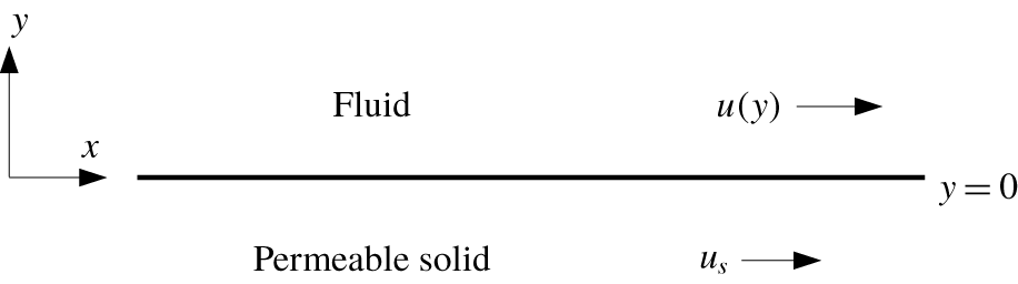
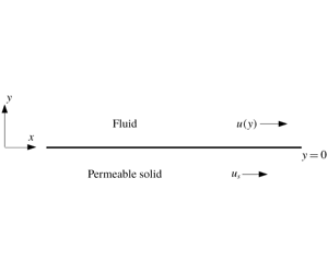
Figure 1. The region
 $y>0$
is occupied by fluid; the region
$y>0$
is occupied by fluid; the region
 $y<0$
is occupied by a permeable solid that oscillates in the
$y<0$
is occupied by a permeable solid that oscillates in the
 $x$
direction with velocity
$x$
direction with velocity
 $\tilde{u} _{s}\text{e}^{\text{i}\unicode[STIX]{x1D714}\tilde{t}}$
.
$\tilde{u} _{s}\text{e}^{\text{i}\unicode[STIX]{x1D714}\tilde{t}}$
.
2 The oscillating plane permeable wall
The problem is two-dimensional, as depicted in figure 1. The region
 ${\tilde{y}}>0$
is occupied by fluid, and the region
${\tilde{y}}>0$
is occupied by fluid, and the region
 ${\tilde{y}}<0$
by a fluid-filled permeable solid that oscillates in the
${\tilde{y}}<0$
by a fluid-filled permeable solid that oscillates in the
 $\tilde{x}$
direction with velocity given by (the real part of)
$\tilde{x}$
direction with velocity given by (the real part of)
 $\tilde{\boldsymbol{u}}_{s}=\tilde{u} _{s}\text{e}^{\text{i}\unicode[STIX]{x1D714}\tilde{t}}\hat{\boldsymbol{x}}$
, where
$\tilde{\boldsymbol{u}}_{s}=\tilde{u} _{s}\text{e}^{\text{i}\unicode[STIX]{x1D714}\tilde{t}}\hat{\boldsymbol{x}}$
, where
 $\unicode[STIX]{x1D714}$
is the angular frequency and
$\unicode[STIX]{x1D714}$
is the angular frequency and
 $\tilde{t}$
is time. The resulting fluid velocity
$\tilde{t}$
is time. The resulting fluid velocity
 $\tilde{u} \text{e}^{\text{i}\unicode[STIX]{x1D714}\tilde{t}}$
is also in the
$\tilde{u} \text{e}^{\text{i}\unicode[STIX]{x1D714}\tilde{t}}$
is also in the
 $\tilde{x}$
direction, with
$\tilde{x}$
direction, with
 $\tilde{u} \rightarrow 0$
as
$\tilde{u} \rightarrow 0$
as
 ${\tilde{y}}\rightarrow \infty$
, and
${\tilde{y}}\rightarrow \infty$
, and
 $\tilde{u}$
tending to a constant as
$\tilde{u}$
tending to a constant as
 ${\tilde{y}}\rightarrow -\infty$
. Thus we have rectilinear flow, and nonlinear terms
${\tilde{y}}\rightarrow -\infty$
. Thus we have rectilinear flow, and nonlinear terms
 $\tilde{\boldsymbol{u}}\boldsymbol{\cdot }\unicode[STIX]{x1D735}\tilde{\boldsymbol{u}}$
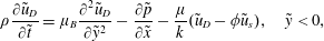
in the Navier–Stokes equation are zero. The fluid has density
$\tilde{\boldsymbol{u}}\boldsymbol{\cdot }\unicode[STIX]{x1D735}\tilde{\boldsymbol{u}}$
in the Navier–Stokes equation are zero. The fluid has density
 $\unicode[STIX]{x1D70C}$
and viscosity
$\unicode[STIX]{x1D70C}$
and viscosity
 $\unicode[STIX]{x1D707}$
. In the upper (fluid) half-space, the fluid velocity
$\unicode[STIX]{x1D707}$
. In the upper (fluid) half-space, the fluid velocity
 $\tilde{u}$
and pressure
$\tilde{u}$
and pressure
 $\tilde{p}$
satisfy
$\tilde{p}$
satisfy
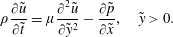 $$\begin{eqnarray}\unicode[STIX]{x1D70C}\frac{\unicode[STIX]{x2202}\tilde{u} }{\unicode[STIX]{x2202}\tilde{t}}=\unicode[STIX]{x1D707}\frac{\unicode[STIX]{x2202}^{2}\tilde{u} }{\unicode[STIX]{x2202}{\tilde{y}}^{2}}-\frac{\unicode[STIX]{x2202}\tilde{p}}{\unicode[STIX]{x2202}\tilde{x}},\quad {\tilde{y}}>0.\end{eqnarray}$$
The fluid is at rest far from the porous solid, with
 $\tilde{u}$
and
$\tilde{u}$
and
 $\unicode[STIX]{x2202}\tilde{p}/\unicode[STIX]{x2202}\tilde{x}$
tending to zero as
$\unicode[STIX]{x2202}\tilde{p}/\unicode[STIX]{x2202}\tilde{x}$
tending to zero as
 ${\tilde{y}}\rightarrow \infty$
. The
${\tilde{y}}\rightarrow \infty$
. The
 ${\tilde{y}}$
component of the Navier–Stokes equations tells us that
${\tilde{y}}$
component of the Navier–Stokes equations tells us that
 $\unicode[STIX]{x2202}\tilde{p}/\unicode[STIX]{x2202}{\tilde{y}}=0$
, and we conclude that
$\unicode[STIX]{x2202}\tilde{p}/\unicode[STIX]{x2202}{\tilde{y}}=0$
, and we conclude that
 $\unicode[STIX]{x1D735}p=0$
everywhere in
$\unicode[STIX]{x1D735}p=0$
everywhere in
 ${\tilde{y}}>0$
.
${\tilde{y}}>0$
.
In the lower half-space, the fluid velocity is again assumed to be solely in the
 $\tilde{x}$
direction. The solid matrix has porosity
$\tilde{x}$
direction. The solid matrix has porosity
 $\unicode[STIX]{x1D719}$
and the mean fluid velocity within the pores is
$\unicode[STIX]{x1D719}$
and the mean fluid velocity within the pores is
 $\langle \tilde{u} \rangle$
(where the average is taken over only the pore space). We set
$\langle \tilde{u} \rangle$
(where the average is taken over only the pore space). We set
 $\tilde{u} _{D}=\unicode[STIX]{x1D719}\langle \tilde{u} \rangle$
, so that when the solid is at rest
$\tilde{u} _{D}=\unicode[STIX]{x1D719}\langle \tilde{u} \rangle$
, so that when the solid is at rest
 $\tilde{u} _{D}$
denotes the Darcy superficial velocity within the porous medium.
$\tilde{u} _{D}$
denotes the Darcy superficial velocity within the porous medium.
Brinkman (Reference Brinkman1947) modified Darcy’s equation by adding a viscous term
 $\unicode[STIX]{x1D707}_{B}\unicode[STIX]{x1D6FB}^{2}\boldsymbol{u}_{D}$
. There is no reason to suppose
$\unicode[STIX]{x1D707}_{B}\unicode[STIX]{x1D6FB}^{2}\boldsymbol{u}_{D}$
. There is no reason to suppose
 $\unicode[STIX]{x1D707}_{B}=\unicode[STIX]{x1D707}$
(as discussed in appendix A), but in §§ 2 and 3 we assume
$\unicode[STIX]{x1D707}_{B}=\unicode[STIX]{x1D707}$
(as discussed in appendix A), but in §§ 2 and 3 we assume
 $\unicode[STIX]{x1D719}=1$
, in which case
$\unicode[STIX]{x1D719}=1$
, in which case
 $\tilde{u} _{D}=\langle \tilde{u} \rangle =\tilde{u}$
and it is generally accepted that
$\tilde{u} _{D}=\langle \tilde{u} \rangle =\tilde{u}$
and it is generally accepted that
 $\unicode[STIX]{x1D707}_{B}=\unicode[STIX]{x1D707}$
is a reasonable assumption. We add a linear inertial term to obtain a Brinkman equation of the form (when the solid matrix is at rest)
$\unicode[STIX]{x1D707}_{B}=\unicode[STIX]{x1D707}$
is a reasonable assumption. We add a linear inertial term to obtain a Brinkman equation of the form (when the solid matrix is at rest)
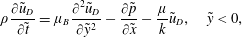 $$\begin{eqnarray}\unicode[STIX]{x1D70C}\frac{\unicode[STIX]{x2202}\tilde{u} _{D}}{\unicode[STIX]{x2202}\tilde{t}}=\unicode[STIX]{x1D707}_{B}\frac{\unicode[STIX]{x2202}^{2}\tilde{u} _{D}}{\unicode[STIX]{x2202}{\tilde{y}}^{2}}-\frac{\unicode[STIX]{x2202}\tilde{p}}{\unicode[STIX]{x2202}\tilde{x}}-\frac{\unicode[STIX]{x1D707}}{k}\tilde{u} _{D},\quad {\tilde{y}}<0,\end{eqnarray}$$
where
 $k$
is the Darcy permeability of the porous medium.
$k$
is the Darcy permeability of the porous medium.
When the solid moves with velocity
 $\tilde{u} _{s}$
, the mean velocity of the fluid relative to the solid matrix is
$\tilde{u} _{s}$
, the mean velocity of the fluid relative to the solid matrix is
 $\langle \tilde{u} \rangle -\tilde{u} _{s}$
and the Darcy drag term is modified to become
$\langle \tilde{u} \rangle -\tilde{u} _{s}$
and the Darcy drag term is modified to become
 $$\begin{eqnarray}\unicode[STIX]{x1D70C}\frac{\unicode[STIX]{x2202}\tilde{u} _{D}}{\unicode[STIX]{x2202}\tilde{t}}=\unicode[STIX]{x1D707}_{B}\frac{\unicode[STIX]{x2202}^{2}\tilde{u} _{D}}{\unicode[STIX]{x2202}{\tilde{y}}^{2}}-\frac{\unicode[STIX]{x2202}\tilde{p}}{\unicode[STIX]{x2202}\tilde{x}}-\frac{\unicode[STIX]{x1D707}}{k}(\tilde{u} _{D}-\unicode[STIX]{x1D719}\tilde{u} _{s}),\quad {\tilde{y}}<0,\end{eqnarray}$$
where
 $\tilde{u} _{D}=\unicode[STIX]{x1D719}\langle \tilde{u} \rangle$
denotes the scaled fluid velocity in the laboratory frame, rather than a Darcy velocity relative to the solid matrix. In the main body of this paper we assume
$\tilde{u} _{D}=\unicode[STIX]{x1D719}\langle \tilde{u} \rangle$
denotes the scaled fluid velocity in the laboratory frame, rather than a Darcy velocity relative to the solid matrix. In the main body of this paper we assume
 $\unicode[STIX]{x1D719}=1$
, so that
$\unicode[STIX]{x1D719}=1$
, so that
 $\tilde{u} _{D}=\langle \tilde{u} \rangle =\tilde{u}$
and
$\tilde{u} _{D}=\langle \tilde{u} \rangle =\tilde{u}$
and
 $\unicode[STIX]{x1D707}_{B}=\unicode[STIX]{x1D707}$
. (We shall relax the assumption
$\unicode[STIX]{x1D707}_{B}=\unicode[STIX]{x1D707}$
. (We shall relax the assumption
 $\unicode[STIX]{x1D719}=1$
in appendix A.) The governing equation (2.3) therefore becomes
$\unicode[STIX]{x1D719}=1$
in appendix A.) The governing equation (2.3) therefore becomes
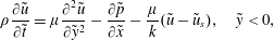 $$\begin{eqnarray}\unicode[STIX]{x1D70C}\frac{\unicode[STIX]{x2202}\tilde{u} }{\unicode[STIX]{x2202}\tilde{t}}=\unicode[STIX]{x1D707}\frac{\unicode[STIX]{x2202}^{2}\tilde{u} }{\unicode[STIX]{x2202}{\tilde{y}}^{2}}-\frac{\unicode[STIX]{x2202}\tilde{p}}{\unicode[STIX]{x2202}\tilde{x}}-\frac{\unicode[STIX]{x1D707}}{k}(\tilde{u} -\tilde{u} _{s}),\quad {\tilde{y}}<0,\end{eqnarray}$$
and
 $\tilde{f}=\unicode[STIX]{x1D707}(\tilde{u} _{s}-\tilde{u} )/k$
is the force per unit volume acting on the fluid due to the Darcy resistance to flow through the porous medium, with
$\tilde{f}=\unicode[STIX]{x1D707}(\tilde{u} _{s}-\tilde{u} )/k$
is the force per unit volume acting on the fluid due to the Darcy resistance to flow through the porous medium, with
 $\tilde{f}=0$
in
$\tilde{f}=0$
in
 ${\tilde{y}}>0$
.
${\tilde{y}}>0$
.
The rectilinear nature of the flow in
 ${\tilde{y}}<0$
ensures (as in
${\tilde{y}}<0$
ensures (as in
 ${\tilde{y}}>0$
) that
${\tilde{y}}>0$
) that
 $\tilde{\boldsymbol{u}}\boldsymbol{\cdot }\unicode[STIX]{x1D735}\tilde{\boldsymbol{u}}$
terms are absent from Brinkman’s equation of motion, and we conclude from the
$\tilde{\boldsymbol{u}}\boldsymbol{\cdot }\unicode[STIX]{x1D735}\tilde{\boldsymbol{u}}$
terms are absent from Brinkman’s equation of motion, and we conclude from the
 ${\tilde{y}}$
component of the equation that
${\tilde{y}}$
component of the equation that
 $\unicode[STIX]{x2202}\tilde{p}/\unicode[STIX]{x2202}{\tilde{y}}=0$
, as in the upper half-plane.
$\unicode[STIX]{x2202}\tilde{p}/\unicode[STIX]{x2202}{\tilde{y}}=0$
, as in the upper half-plane.
As is usual in one-domain models, we assume that the fluid velocity
 $\tilde{u}$
, shear stress
$\tilde{u}$
, shear stress
 $\unicode[STIX]{x1D707}\unicode[STIX]{x2202}\tilde{u} /\unicode[STIX]{x2202}{\tilde{y}}$
and pressure
$\unicode[STIX]{x1D707}\unicode[STIX]{x2202}\tilde{u} /\unicode[STIX]{x2202}{\tilde{y}}$
and pressure
 $\tilde{p}$
are continuous at
$\tilde{p}$
are continuous at
 $y=0$
. There are therefore no pressure gradients in this uni-directional flow, so from henceforth we set
$y=0$
. There are therefore no pressure gradients in this uni-directional flow, so from henceforth we set
 $\tilde{p}=0$
. If we multiply the governing equations (2.1) and (2.4) by
$\tilde{p}=0$
. If we multiply the governing equations (2.1) and (2.4) by
 $\tilde{u}$
and integrate (2.4) over
$\tilde{u}$
and integrate (2.4) over
 $-\tilde{L}<{\tilde{y}}<0$
and (2.1) over
$-\tilde{L}<{\tilde{y}}<0$
and (2.1) over
 $0<{\tilde{y}}<\tilde{M}$
, we obtain the energy equation
$0<{\tilde{y}}<\tilde{M}$
, we obtain the energy equation
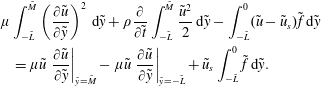 $$\begin{eqnarray}\displaystyle & & \displaystyle \unicode[STIX]{x1D707}\int _{-\tilde{L}}^{\tilde{M}}\left(\frac{\unicode[STIX]{x2202}\tilde{u} }{\unicode[STIX]{x2202}{\tilde{y}}}\right)^{2}\,\text{d}{\tilde{y}}+\unicode[STIX]{x1D70C}\frac{\unicode[STIX]{x2202}}{\unicode[STIX]{x2202}\tilde{t}}\int _{-\tilde{L}}^{\tilde{M}}\frac{\tilde{u} ^{2}}{2}\,\text{d}{\tilde{y}}-\int _{-\tilde{L}}^{0}(\tilde{u} -\tilde{u} _{s})\tilde{f}\,\text{d}{\tilde{y}}\nonumber\\ \displaystyle & & \displaystyle \quad =\unicode[STIX]{x1D707}\tilde{u} \left.\frac{\unicode[STIX]{x2202}\tilde{u} }{\unicode[STIX]{x2202}{\tilde{y}}}\right|_{{\tilde{y}}=\tilde{M}}-\unicode[STIX]{x1D707}\tilde{u} \left.\frac{\unicode[STIX]{x2202}\tilde{u} }{\unicode[STIX]{x2202}{\tilde{y}}}\right|_{{\tilde{y}}=-\tilde{L}}+\tilde{u} _{s}\int _{-\tilde{L}}^{0}\tilde{f}\,\text{d}{\tilde{y}}.\end{eqnarray}$$
The right-hand side of (2.5) represents the rate of input of energy by the solid matrix in
 ${\tilde{y}}<0$
as it moves with velocity
${\tilde{y}}<0$
as it moves with velocity
 $\tilde{u} _{s}$
, together with any work performed at the upper and lower boundaries
$\tilde{u} _{s}$
, together with any work performed at the upper and lower boundaries
 ${\tilde{y}}=\tilde{M}$
,
${\tilde{y}}=\tilde{M}$
,
 ${\tilde{y}}=-\tilde{L}$
. These boundary terms tend to zero as we allow
${\tilde{y}}=-\tilde{L}$
. These boundary terms tend to zero as we allow
 $\tilde{L}$
and
$\tilde{L}$
and
 $\tilde{M}$
to tend to infinity. The left-hand side of (2.5) represents viscous dissipation due to shear within both the permeable medium and the adjacent fluid, the rate of change of kinetic energy of the fluid, and the rate at which the motion of the fluid relative to the solid matrix performs work. The rate at which the solid performs work on the liquid determines the rate of damping of interest to Kang et al. (Reference Kang, Dehdashti, Vandadi and Masoud2019), and we therefore direct our attention to this final term on the right-hand side of (2.5).
$\tilde{M}$
to tend to infinity. The left-hand side of (2.5) represents viscous dissipation due to shear within both the permeable medium and the adjacent fluid, the rate of change of kinetic energy of the fluid, and the rate at which the motion of the fluid relative to the solid matrix performs work. The rate at which the solid performs work on the liquid determines the rate of damping of interest to Kang et al. (Reference Kang, Dehdashti, Vandadi and Masoud2019), and we therefore direct our attention to this final term on the right-hand side of (2.5).
We look for oscillatory solutions in which all quantities vary as
 $\text{e}^{\text{i}\unicode[STIX]{x1D714}\tilde{t}}$
, and from now on drop explicit mention of this exponential factor. We scale time by
$\text{e}^{\text{i}\unicode[STIX]{x1D714}\tilde{t}}$
, and from now on drop explicit mention of this exponential factor. We scale time by
 $\unicode[STIX]{x1D714}^{-1}$
, lengths in the
$\unicode[STIX]{x1D714}^{-1}$
, lengths in the
 $y$
direction by
$y$
direction by
 $L_{d}=(\unicode[STIX]{x1D707}/\unicode[STIX]{x1D70C}\unicode[STIX]{x1D714})^{1/2}$
(the length scale for diffusion of vorticity), velocities by
$L_{d}=(\unicode[STIX]{x1D707}/\unicode[STIX]{x1D70C}\unicode[STIX]{x1D714})^{1/2}$
(the length scale for diffusion of vorticity), velocities by
 $\tilde{u} _{s}$
, stress by
$\tilde{u} _{s}$
, stress by
 $\unicode[STIX]{x1D707}\tilde{u} _{s}/L_{d}$
and force per unit volume by
$\unicode[STIX]{x1D707}\tilde{u} _{s}/L_{d}$
and force per unit volume by
 $\unicode[STIX]{x1D707}\tilde{u} _{s}/L_{d}^{2}$
, and we denote non-dimensional quantities by the absence of a tilde. There are no pressure gradients. The governing equations become
$\unicode[STIX]{x1D707}\tilde{u} _{s}/L_{d}^{2}$
, and we denote non-dimensional quantities by the absence of a tilde. There are no pressure gradients. The governing equations become
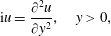
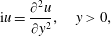 $$\begin{eqnarray}\displaystyle & \displaystyle \text{i}u=\frac{\unicode[STIX]{x2202}^{2}u}{\unicode[STIX]{x2202}y^{2}},\quad y>0, & \displaystyle\end{eqnarray}$$
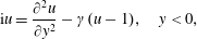 $$\begin{eqnarray}\displaystyle & \displaystyle \text{i}u=\frac{\unicode[STIX]{x2202}^{2}u}{\unicode[STIX]{x2202}y^{2}}-\unicode[STIX]{x1D6FE}(u-1),\quad y<0, & \displaystyle\end{eqnarray}$$
 $$\begin{eqnarray}\unicode[STIX]{x1D6FE}=\frac{L_{d}^{2}}{k}=\frac{\unicode[STIX]{x1D707}}{\unicode[STIX]{x1D70C}\unicode[STIX]{x1D714}k}.\end{eqnarray}$$
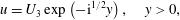
The solution of this pair of equations is straightforward, with
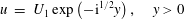 $$\begin{eqnarray}\displaystyle u & = & \displaystyle U_{1}\exp \left(-\text{i}^{1/2}y\right),\quad y>0\end{eqnarray}$$
 $$\begin{eqnarray}\displaystyle & = & \displaystyle \frac{\unicode[STIX]{x1D6FE}}{\unicode[STIX]{x1D6FE}+\text{i}}+U_{2}\exp \left((\unicode[STIX]{x1D6FE}+\text{i})^{1/2}y\right),\quad y<0,\end{eqnarray}$$
 $\text{i}^{1/2}$
and
$\text{i}^{1/2}$
and
 $(\unicode[STIX]{x1D6FE}+\text{i})^{1/2}$
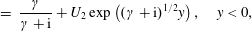
are chosen to have positive real part. Continuity of the fluid velocity and shear stress at
$(\unicode[STIX]{x1D6FE}+\text{i})^{1/2}$
are chosen to have positive real part. Continuity of the fluid velocity and shear stress at
 $y=0$
requires
$y=0$
requires 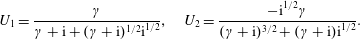 $$\begin{eqnarray}U_{1}=\frac{\unicode[STIX]{x1D6FE}}{\unicode[STIX]{x1D6FE}+\text{i}+(\unicode[STIX]{x1D6FE}+\text{i})^{1/2}\text{i}^{1/2}},\quad U_{2}=\frac{-\text{i}^{1/2}\unicode[STIX]{x1D6FE}}{(\unicode[STIX]{x1D6FE}+\text{i})^{3/2}+(\unicode[STIX]{x1D6FE}+\text{i})\text{i}^{1/2}}.\end{eqnarray}$$
The non-dimensional force that the solid exerts on the fluid is
 $f=\unicode[STIX]{x1D6FE}(1-u)$
per unit volume, so that the rate of working of the solid as it oscillates with non-dimensional velocity
$f=\unicode[STIX]{x1D6FE}(1-u)$
per unit volume, so that the rate of working of the solid as it oscillates with non-dimensional velocity
 $\text{Re}\{\text{e}^{\text{i}t}\}$
is
$\text{Re}\{\text{e}^{\text{i}t}\}$
is
 $$\begin{eqnarray}W(y,t)=\unicode[STIX]{x1D6FE}\text{Re}\left\{\left[1-\frac{\unicode[STIX]{x1D6FE}}{\unicode[STIX]{x1D6FE}+\text{i}}-U_{2}\exp \left((\unicode[STIX]{x1D6FE}+\text{i})^{1/2}y\right)\right]\text{e}^{\text{i}t}\right\}\text{Re}\left\{\text{e}^{\text{i}t}\right\}\end{eqnarray}$$
and the mean rate of working is
 $$\begin{eqnarray}\overline{W}(y)=\frac{1}{2\unicode[STIX]{x03C0}}\int _{0}^{2\unicode[STIX]{x03C0}}W(y,t)\,\text{d}t=\frac{\unicode[STIX]{x1D6FE}}{2(\unicode[STIX]{x1D6FE}^{2}+1)}-\frac{\unicode[STIX]{x1D6FE}}{2}\text{Re}\left\{U_{2}\exp ((\unicode[STIX]{x1D6FE}+\text{i})^{1/2}y)\right\}.\end{eqnarray}$$
Fluid inertia prevents the pore fluid from moving with the velocity of the solid, so that, by (2.8b
),
 $u\rightarrow \unicode[STIX]{x1D6FE}/(\unicode[STIX]{x1D6FE}+\text{i})$
as
$u\rightarrow \unicode[STIX]{x1D6FE}/(\unicode[STIX]{x1D6FE}+\text{i})$
as
 $y\rightarrow -\infty$
, representing a fluid velocity that oscillates out of phase relative to the solid matrix. As a result, the rate of working of the solid matrix, per unit volume, tends to a non-zero constant as
$y\rightarrow -\infty$
, representing a fluid velocity that oscillates out of phase relative to the solid matrix. As a result, the rate of working of the solid matrix, per unit volume, tends to a non-zero constant as
 $y\rightarrow -\infty$
. The depth-integrated mean rate of working of the solid in the region
$y\rightarrow -\infty$
. The depth-integrated mean rate of working of the solid in the region
 $-L<y<0$
, with
$-L<y<0$
, with
 $L\gg \unicode[STIX]{x1D6FE}^{-1/2}$
, is
$L\gg \unicode[STIX]{x1D6FE}^{-1/2}$
, is
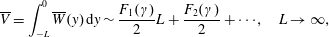 $$\begin{eqnarray}\overline{V}=\int _{-L}^{0}\overline{W}(y)\,\text{d}y\sim \frac{F_{1}(\unicode[STIX]{x1D6FE})}{2}L+\frac{F_{2}(\unicode[STIX]{x1D6FE})}{2}+\cdots \!,\quad L\rightarrow \infty ,\end{eqnarray}$$
where
 $$\begin{eqnarray}F_{1}(\unicode[STIX]{x1D6FE})=\frac{\unicode[STIX]{x1D6FE}}{\unicode[STIX]{x1D6FE}^{2}+1}\end{eqnarray}$$
and
 $$\begin{eqnarray}F_{2}(\unicode[STIX]{x1D6FE})=-\unicode[STIX]{x1D6FE}\text{Re}\left\{\int _{-\infty }^{0}U_{2}\exp \left((\unicode[STIX]{x1D6FE}+\text{i})^{1/2}y\right)\,\text{d}y\right\}=\text{Re}\left\{\frac{\text{i}^{1/2}\unicode[STIX]{x1D6FE}^{2}}{(\unicode[STIX]{x1D6FE}+\text{i})^{2}+(\unicode[STIX]{x1D6FE}+\text{i})^{3/2}\text{i}^{1/2}}\right\}.\end{eqnarray}$$
In dimensional form, the total mean rate of working (per unit length in the
 $x$
direction) by the solid matrix is
$x$
direction) by the solid matrix is
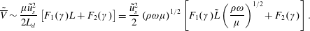 $$\begin{eqnarray}\tilde{\overline{V}}\sim \frac{\unicode[STIX]{x1D707}\tilde{u} _{s}^{2}}{2L_{d}}\left[F_{1}(\unicode[STIX]{x1D6FE})L+F_{2}(\unicode[STIX]{x1D6FE})\right]=\frac{\tilde{u} _{s}^{2}}{2}\left(\unicode[STIX]{x1D70C}\unicode[STIX]{x1D714}\unicode[STIX]{x1D707}\right)^{1/2}\left[F_{1}(\unicode[STIX]{x1D6FE})\tilde{L}\left(\frac{\unicode[STIX]{x1D70C}\unicode[STIX]{x1D714}}{\unicode[STIX]{x1D707}}\right)^{1/2}+F_{2}(\unicode[STIX]{x1D6FE})\right].\end{eqnarray}$$
If we allow the permeability
 $k$
to tend to zero, so that
$k$
to tend to zero, so that
 $\unicode[STIX]{x1D6FE}=L_{d}^{2}/k\rightarrow \infty$
, then
$\unicode[STIX]{x1D6FE}=L_{d}^{2}/k\rightarrow \infty$
, then
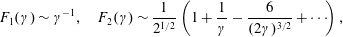 $$\begin{eqnarray}F_{1}(\unicode[STIX]{x1D6FE})\sim \unicode[STIX]{x1D6FE}^{-1},\quad F_{2}(\unicode[STIX]{x1D6FE})\sim \frac{1}{2^{1/2}}\left(1+\frac{1}{\unicode[STIX]{x1D6FE}}-\frac{6}{(2\unicode[STIX]{x1D6FE})^{3/2}}+\cdots \!\right),\end{eqnarray}$$
and as
 $\unicode[STIX]{x1D6FE}\rightarrow \infty$
the total rate of working tends towards the classical result for the rate of dissipation in fluid adjacent to an oscillating plane impermeable wall. In this limit, fluid within the permeable solid moves at almost the same velocity as the solid, except within a boundary layer of thickness
$\unicode[STIX]{x1D6FE}\rightarrow \infty$
the total rate of working tends towards the classical result for the rate of dissipation in fluid adjacent to an oscillating plane impermeable wall. In this limit, fluid within the permeable solid moves at almost the same velocity as the solid, except within a boundary layer of thickness
 $\unicode[STIX]{x1D6FE}^{-1/2}$
, within which the relative velocity is
$\unicode[STIX]{x1D6FE}^{-1/2}$
, within which the relative velocity is
 $O(\unicode[STIX]{x1D6FE}^{-1/2})$
, shear rates are
$O(\unicode[STIX]{x1D6FE}^{-1/2})$
, shear rates are
 $O(1)$
and the force
$O(1)$
and the force
 $f$
is
$f$
is
 $O(\unicode[STIX]{x1D6FE}^{1/2})$
. In consequence, the energy equation (2.5) represents a large force
$O(\unicode[STIX]{x1D6FE}^{1/2})$
. In consequence, the energy equation (2.5) represents a large force
 $\tilde{f}$
confined to a thin boundary layer at the surface of the permeable solid, balanced by dissipation almost entirely within the unbounded fluid in
$\tilde{f}$
confined to a thin boundary layer at the surface of the permeable solid, balanced by dissipation almost entirely within the unbounded fluid in
 $y>0$
, together with an oscillating kinetic energy term.
$y>0$
, together with an oscillating kinetic energy term.
As
 $\unicode[STIX]{x1D6FE}\rightarrow 0$
,
$\unicode[STIX]{x1D6FE}\rightarrow 0$
,
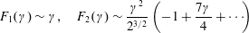 $$\begin{eqnarray}F_{1}(\unicode[STIX]{x1D6FE})\sim \unicode[STIX]{x1D6FE},\quad F_{2}(\unicode[STIX]{x1D6FE})\sim \frac{\unicode[STIX]{x1D6FE}^{2}}{2^{3/2}}\left(-1+\frac{7\unicode[STIX]{x1D6FE}}{4}+\cdots \!\right)\end{eqnarray}$$
and the highly permeable porous solid exerts little force on the fluid, which in consequence hardly moves. We plot the functions
 $F_{1}(\unicode[STIX]{x1D6FE})$
and
$F_{1}(\unicode[STIX]{x1D6FE})$
and
 $F_{2}(\unicode[STIX]{x1D6FE})$
in figure 2. We see that
$F_{2}(\unicode[STIX]{x1D6FE})$
in figure 2. We see that
 $F_{1}$
, associated with work performed within the interior of the porous slab, has a maximum at
$F_{1}$
, associated with work performed within the interior of the porous slab, has a maximum at
 $\unicode[STIX]{x1D6FE}=1$
, whereas
$\unicode[STIX]{x1D6FE}=1$
, whereas
 $F_{2}$
, associated with the region near the boundary at
$F_{2}$
, associated with the region near the boundary at
 $y=0$
, is not far from monotonic apart from a small overshoot near
$y=0$
, is not far from monotonic apart from a small overshoot near
 $\unicode[STIX]{x1D6FE}=10$
and a small undershoot near
$\unicode[STIX]{x1D6FE}=10$
and a small undershoot near
 $\unicode[STIX]{x1D6FE}=0.4$
. If the porous slab has thickness
$\unicode[STIX]{x1D6FE}=0.4$
. If the porous slab has thickness
 $L\gg \unicode[STIX]{x1D6FE}^{-1/2}$
the total rate of working of the solid (2.15) is dominated by the term
$L\gg \unicode[STIX]{x1D6FE}^{-1/2}$
the total rate of working of the solid (2.15) is dominated by the term
 $LF_{1}(\unicode[STIX]{x1D6FE})$
and exhibits a maximum near
$LF_{1}(\unicode[STIX]{x1D6FE})$
and exhibits a maximum near
 $\unicode[STIX]{x1D6FE}=1$
. If
$\unicode[STIX]{x1D6FE}=1$
. If
 $L\ll \unicode[STIX]{x1D6FE}^{-1/2}$
we expect the surface effects to play a dominant role. However, if the porous layer is shallow the expansion (2.12) for the mean rate of working when
$L\ll \unicode[STIX]{x1D6FE}^{-1/2}$
we expect the surface effects to play a dominant role. However, if the porous layer is shallow the expansion (2.12) for the mean rate of working when
 $L\gg \unicode[STIX]{x1D6FE}^{-1/2}$
is no longer valid, and we cannot ignore boundary conditions at
$L\gg \unicode[STIX]{x1D6FE}^{-1/2}$
is no longer valid, and we cannot ignore boundary conditions at
 $y=-L$
. One could investigate this limit by setting up an alternative geometry e.g. a symmetric problem with a porous slab occupying the region
$y=-L$
. One could investigate this limit by setting up an alternative geometry e.g. a symmetric problem with a porous slab occupying the region
 $-H<y<H$
, with fluid in the regions
$-H<y<H$
, with fluid in the regions
 $|y|>H$
, but we shall not pursue this.
$|y|>H$
, but we shall not pursue this.


3 Impulsive start-up from rest of a permeable wall
Stokes’ (Reference Stokes1851) analysis of fluid motion adjacent to a plane wall that starts to move impulsively in its own plane with a steady velocity
 $\tilde{U} _{s}H(t)$
(where
$\tilde{U} _{s}H(t)$
(where
 $H(t)$
is the Heaviside function) is a second textbook example taught to undergraduates (Batchelor Reference Batchelor1973). We again investigate the effect of replacing the plane wall at
$H(t)$
is the Heaviside function) is a second textbook example taught to undergraduates (Batchelor Reference Batchelor1973). We again investigate the effect of replacing the plane wall at
 ${\tilde{y}}=0$
by a permeable half-space
${\tilde{y}}=0$
by a permeable half-space
 ${\tilde{y}}<0$
.
${\tilde{y}}<0$
.
The fluid is at rest at time
 $\tilde{t}=0$
, and subsequently moves with velocity
$\tilde{t}=0$
, and subsequently moves with velocity
 $\tilde{u} (\tilde{t},{\tilde{y}})$
in the
$\tilde{u} (\tilde{t},{\tilde{y}})$
in the
 $\tilde{x}$
direction. Fluid motion in the region
$\tilde{x}$
direction. Fluid motion in the region
 ${\tilde{y}}>0$
obeys the Navier–Stokes equation (2.1); in the region
${\tilde{y}}>0$
obeys the Navier–Stokes equation (2.1); in the region
 ${\tilde{y}}<0$
it obeys the Brinkman equation (2.4). As in § 2, pressure gradients are zero, so we set
${\tilde{y}}<0$
it obeys the Brinkman equation (2.4). As in § 2, pressure gradients are zero, so we set
 $\tilde{p}=0$
.
$\tilde{p}=0$
.
We scale velocities by
 $\tilde{U} _{s}$
, and for the moment we scale lengths in the
$\tilde{U} _{s}$
, and for the moment we scale lengths in the
 $y$
direction by an arbitrary length scale
$y$
direction by an arbitrary length scale
 $\tilde{L}$
. Time is scaled by
$\tilde{L}$
. Time is scaled by
 $\tilde{L}^{2}\unicode[STIX]{x1D70C}/\unicode[STIX]{x1D707}$
, stress by
$\tilde{L}^{2}\unicode[STIX]{x1D70C}/\unicode[STIX]{x1D707}$
, stress by
 $\unicode[STIX]{x1D707}\tilde{U} _{s}/\tilde{L}$
, force per unit volume by
$\unicode[STIX]{x1D707}\tilde{U} _{s}/\tilde{L}$
, force per unit volume by
 $\unicode[STIX]{x1D707}\tilde{U} _{s}/\tilde{L}^{2}$
and we denote non-dimensional quantities by the absence of a tilde. The governing equations become
$\unicode[STIX]{x1D707}\tilde{U} _{s}/\tilde{L}^{2}$
and we denote non-dimensional quantities by the absence of a tilde. The governing equations become
 $$\begin{eqnarray}\displaystyle & \displaystyle \frac{\unicode[STIX]{x2202}u}{\unicode[STIX]{x2202}t}=\frac{\unicode[STIX]{x2202}^{2}u}{\unicode[STIX]{x2202}y^{2}},\quad y>0, & \displaystyle\end{eqnarray}$$
 $$\begin{eqnarray}\displaystyle & \displaystyle \frac{\unicode[STIX]{x2202}u}{\unicode[STIX]{x2202}t}=\frac{\unicode[STIX]{x2202}^{2}u}{\unicode[STIX]{x2202}y^{2}}-R(u-u_{s}),\quad y<0, & \displaystyle\end{eqnarray}$$
 $R=\tilde{L}^{2}/k$
and the non-dimensional solid velocity
$R=\tilde{L}^{2}/k$
and the non-dimensional solid velocity
 $u_{s}=H(t)$
. We take Laplace transforms, with
$u_{s}=H(t)$
. We take Laplace transforms, with  $$\begin{eqnarray}u^{\ast }(s,y)=\int _{0}^{\infty }u(t,y)\text{e}^{-st}\,\text{d}t.\end{eqnarray}$$
The governing equations become
 $$\begin{eqnarray}\displaystyle & \displaystyle su^{\ast }=\frac{\unicode[STIX]{x2202}^{2}u^{\ast }}{\unicode[STIX]{x2202}y^{2}},\quad y>0, & \displaystyle\end{eqnarray}$$
 $$\begin{eqnarray}\displaystyle & \displaystyle su^{\ast }=\frac{\unicode[STIX]{x2202}^{2}u^{\ast }}{\unicode[STIX]{x2202}y^{2}}-R\left(u^{\ast }-\frac{1}{s}\right),\quad y<0, & \displaystyle\end{eqnarray}$$
 $$\begin{eqnarray}\displaystyle & \displaystyle u^{\ast }=A(s)\exp \left(-s^{1/2}y\right),\quad y>0, & \displaystyle\end{eqnarray}$$
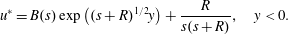 $$\begin{eqnarray}\displaystyle & \displaystyle u^{\ast }=B(s)\exp \left((s+R)^{1/2}y\right)+\frac{R}{s(s+R)},\quad y<0. & \displaystyle\end{eqnarray}$$
 $u^{\ast }$
and shear stress
$u^{\ast }$
and shear stress
 $\unicode[STIX]{x2202}u^{\ast }/\unicode[STIX]{x2202}y$
at
$\unicode[STIX]{x2202}u^{\ast }/\unicode[STIX]{x2202}y$
at
 $y=0$
gives
$y=0$
gives  $$\begin{eqnarray}A=\frac{R}{s(s+R)^{1/2}[(s+R)^{1/2}+s^{1/2}]},\quad B=-\frac{R}{s^{1/2}(s+R)[(s+R)^{1/2}+s^{1/2}]}.\end{eqnarray}$$
The fluid velocity in the permeable medium far from the interface (
 $y\rightarrow -\infty$
) depends solely on a balance between inertia and the Darcy resistance to flow, with
$y\rightarrow -\infty$
) depends solely on a balance between inertia and the Darcy resistance to flow, with
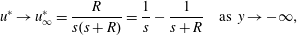 $$\begin{eqnarray}u^{\ast }\rightarrow u_{\infty }^{\ast }=\frac{R}{s(s+R)}=\frac{1}{s}-\frac{1}{s+R}\quad \text{as }y\rightarrow -\infty ,\end{eqnarray}$$
corresponding to
 $$\begin{eqnarray}u\rightarrow u_{\infty }=1-\exp (-Rt).\end{eqnarray}$$
The non-dimensional force that the solid exerts on the fluid is
 $f=R(1-u)$
per unit volume. In an unbounded porous medium this force would be
$f=R(1-u)$
per unit volume. In an unbounded porous medium this force would be
 $R(1-u_{\infty })=R\exp (-Rt)$
. The total additional force (per unit length in the
$R(1-u_{\infty })=R\exp (-Rt)$
. The total additional force (per unit length in the
 $x$
direction) due to the presence of the interface at
$x$
direction) due to the presence of the interface at
 $y=0$
is therefore
$y=0$
is therefore
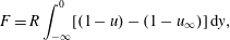 $$\begin{eqnarray}F=R\int _{-\infty }^{0}[(1-u)-(1-u_{\infty })]\,\text{d}y,\end{eqnarray}$$
with Laplace transform
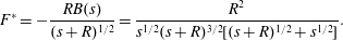 $$\begin{eqnarray}F^{\ast }=-\frac{RB(s)}{(s+R)^{1/2}}=\frac{R^{2}}{s^{1/2}(s+R)^{3/2}[(s+R)^{1/2}+s^{1/2}]}.\end{eqnarray}$$
In the limit of an impermeable solid (
 $k\rightarrow 0$
,
$k\rightarrow 0$
,
 $R=\tilde{L}^{2}/k\rightarrow \infty$
), for fixed
$R=\tilde{L}^{2}/k\rightarrow \infty$
), for fixed
 $s$
we find
$s$
we find
 $F^{\ast }\sim s^{-1/2}$
corresponding to non-dimensional and dimensional forces
$F^{\ast }\sim s^{-1/2}$
corresponding to non-dimensional and dimensional forces
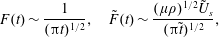 $$\begin{eqnarray}F(t)\sim \frac{1}{(\unicode[STIX]{x03C0}t)^{1/2}},\quad \tilde{F}(t)\sim \frac{(\unicode[STIX]{x1D707}\unicode[STIX]{x1D70C})^{1/2}\tilde{U} _{s}}{(\unicode[STIX]{x03C0}\tilde{t})^{1/2}},\end{eqnarray}$$
in agreement with the classical result for impulsive start-up from rest of an impermeable solid surface.
For more general
 $R$
, the transform pairs (Abramowitz & Stegun Reference Abramowitz and Stegun1972)
$R$
, the transform pairs (Abramowitz & Stegun Reference Abramowitz and Stegun1972)
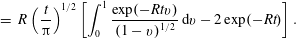
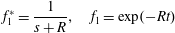 $$\begin{eqnarray}f_{1}^{\ast }=\frac{1}{s+R},\quad f_{1}=\exp (-Rt)\end{eqnarray}$$
and
 $$\begin{eqnarray}f_{2}^{\ast }=\frac{1}{s^{1/2}(s+R)^{1/2}[(s+R)^{1/2}+s^{1/2}]},\quad f_{2}=\frac{1}{R^{1/2}}\exp (-Rt/2)\text{I}_{1/2}(Rt/2)\end{eqnarray}$$
(where
 $\text{I}_{1/2}(z)=\sinh (z)(2/\unicode[STIX]{x03C0}z)^{1/2}$
is a modified Bessel function) can be combined to find the inverse transform of
$\text{I}_{1/2}(z)=\sinh (z)(2/\unicode[STIX]{x03C0}z)^{1/2}$
is a modified Bessel function) can be combined to find the inverse transform of
 $F^{\ast }$
(3.9), with
$F^{\ast }$
(3.9), with
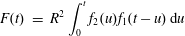 $$\begin{eqnarray}\displaystyle F(t) & = & \displaystyle R^{2}\int _{0}^{t}f_{2}(u)f_{1}(t-u)\,\text{d}u\end{eqnarray}$$
 $$\begin{eqnarray}\displaystyle & = & \displaystyle R\left(\frac{t}{\unicode[STIX]{x03C0}}\right)^{1/2}\left[\int _{0}^{1}\frac{\exp (-Rtv)}{(1-v)^{1/2}}\,\text{d}v-2\exp (-Rt)\right].\end{eqnarray}$$
When
 $Rt\ll 1$
we expand the exponential in (3.14) to obtain
$Rt\ll 1$
we expand the exponential in (3.14) to obtain
 $$\begin{eqnarray}F\sim \frac{2R^{2}t^{3/2}}{3\unicode[STIX]{x03C0}^{1/2}}-\frac{7R^{3}t^{5/2}}{15\unicode[STIX]{x03C0}^{1/2}}+\cdots \!,\end{eqnarray}$$
which could alternatively have been obtained by inverting term-by-term the expansion of
 $F^{\ast }$
(3.9) in the limit
$F^{\ast }$
(3.9) in the limit
 $s\rightarrow \infty$
 $$\begin{eqnarray}F^{\ast }\sim \frac{R^{2}}{2s^{5/2}}\left(1-\frac{7R}{4s}+\cdots \,\right)\!.\end{eqnarray}$$
The
 $t^{-1/2}$
singularity (3.10) when
$t^{-1/2}$
singularity (3.10) when
 $k=0$
has been removed. When
$k=0$
has been removed. When
 $Rt\gg 1$
we expand
$Rt\gg 1$
we expand
 $(1-v)^{-1/2}$
in (3.14) as a power series for small
$(1-v)^{-1/2}$
in (3.14) as a power series for small
 $v$
, to obtain
$v$
, to obtain
 $$\begin{eqnarray}F\sim \frac{1}{(\unicode[STIX]{x03C0}t)^{1/2}}+\frac{1}{2R\unicode[STIX]{x03C0}^{1/2}t^{3/2}}+\cdots \!.\end{eqnarray}$$


We now pick the length scale
 $L=k^{1/2}$
, so that
$L=k^{1/2}$
, so that
 $R=1$
. (The only reason for not adopting this natural choice straight away was so that we could consider the limit
$R=1$
. (The only reason for not adopting this natural choice straight away was so that we could consider the limit
 $k=0$
and thereby obtain (3.10).) Figure 3 shows the force
$k=0$
and thereby obtain (3.10).) Figure 3 shows the force
 $F$
(3.14), together with the asymptotes for
$F$
(3.14), together with the asymptotes for
 $t\ll 1$
(3.15), and
$t\ll 1$
(3.15), and
 $t\gg 1$
(3.17).
$t\gg 1$
(3.17).
The Laplace transform of the velocity on
 $y=0$
is
$y=0$
is
 $u^{\ast }(s,y=0)=A(s)$
, given by (3.5). To invert this, we note that the Laplace transform pair
$u^{\ast }(s,y=0)=A(s)$
, given by (3.5). To invert this, we note that the Laplace transform pair
 $$\begin{eqnarray}f_{3}^{\ast }=\frac{1}{s^{1/2}},\quad f_{3}=\frac{1}{(\unicode[STIX]{x03C0}t)^{1/2}}\end{eqnarray}$$
can be combined with the pair (3.12) to give
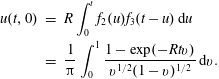 $$\begin{eqnarray}\displaystyle u(t,0) & = & \displaystyle R\int _{0}^{t}f_{2}(u)f_{3}(t-u)\,\text{d}u\nonumber\\ \displaystyle & = & \displaystyle \frac{1}{\unicode[STIX]{x03C0}}\int _{0}^{1}\frac{1-\exp (-Rtv)}{v^{1/2}(1-v)^{1/2}}\,\text{d}v.\end{eqnarray}$$
When
 $Rt\ll 1$
, we expand the exponential in (3.19) to obtain
$Rt\ll 1$
, we expand the exponential in (3.19) to obtain
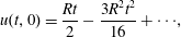 $$\begin{eqnarray}u(t,0)=\frac{Rt}{2}-\frac{3R^{2}t^{2}}{16}+\cdots \!,\end{eqnarray}$$
which can be obtained alternatively by inverting term-by-term the expansion of
 $A(s)$
for
$A(s)$
for
 $s\gg R$
. We see that non-zero permeability smooths out the step change in fluid velocity that occurs adjacent to an impermeable surface at
$s\gg R$
. We see that non-zero permeability smooths out the step change in fluid velocity that occurs adjacent to an impermeable surface at
 $t=0$
. When
$t=0$
. When
 $Rt\gg 1$
,
$Rt\gg 1$
,
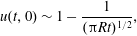 $$\begin{eqnarray}u(t,0)\sim 1-\frac{1}{(\unicode[STIX]{x03C0}Rt)^{1/2}},\end{eqnarray}$$
and the expansion of (3.4b
) for
 $s\ll R$
leads to
$s\ll R$
leads to
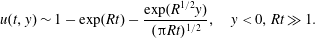 $$\begin{eqnarray}u(t,y)\sim 1-\exp (Rt)-\frac{\exp (R^{1/2}y)}{(\unicode[STIX]{x03C0}Rt)^{1/2}},\quad y<0,Rt\gg 1.\end{eqnarray}$$
4 Concluding remarks
The above Brinkman analysis includes an inertial
 $\unicode[STIX]{x1D70C}\,\unicode[STIX]{x2202}\boldsymbol{u}/\unicode[STIX]{x2202}t$
term, but studies of high Reynolds number flow inside model porous media have shown that nonlinear
$\unicode[STIX]{x1D70C}\,\unicode[STIX]{x2202}\boldsymbol{u}/\unicode[STIX]{x2202}t$
term, but studies of high Reynolds number flow inside model porous media have shown that nonlinear
 $\unicode[STIX]{x1D70C}\,\boldsymbol{u}\boldsymbol{\cdot }\unicode[STIX]{x1D735}\boldsymbol{u}$
inertial contributions due to tortuosity can be important within the porous medium, even when Darcy flow is nominally rectilinear (Mei & Auriault Reference Mei and Auriault1991; Koch & Hill Reference Koch and Hill2001; Graham & Higdon Reference Graham and Higdon2002) and such nonlinear terms are absent from the Brinkman equation (2.4). A recent study by Lasseux, Valdés-Parada & Bellet (Reference Lasseux, Valdés-Parada and Bellet2019) of high Reynolds number unsteady flow in a porous medium (of porosity 0.4) compared direct numerical simulations and an upscaling model against a heuristic model based solely on the fluid inertia
$\unicode[STIX]{x1D70C}\,\boldsymbol{u}\boldsymbol{\cdot }\unicode[STIX]{x1D735}\boldsymbol{u}$
inertial contributions due to tortuosity can be important within the porous medium, even when Darcy flow is nominally rectilinear (Mei & Auriault Reference Mei and Auriault1991; Koch & Hill Reference Koch and Hill2001; Graham & Higdon Reference Graham and Higdon2002) and such nonlinear terms are absent from the Brinkman equation (2.4). A recent study by Lasseux, Valdés-Parada & Bellet (Reference Lasseux, Valdés-Parada and Bellet2019) of high Reynolds number unsteady flow in a porous medium (of porosity 0.4) compared direct numerical simulations and an upscaling model against a heuristic model based solely on the fluid inertia
 $\unicode[STIX]{x1D70C}\,\unicode[STIX]{x2202}\boldsymbol{u}/\unicode[STIX]{x2202}t$
and the steady Darcy permeability. The heuristic model, equivalent to Brinkman’s equation when flow is unidirectional, overestimated the effect of oscillatory pressure gradient fluctuations by a factor
$\unicode[STIX]{x1D70C}\,\unicode[STIX]{x2202}\boldsymbol{u}/\unicode[STIX]{x2202}t$
and the steady Darcy permeability. The heuristic model, equivalent to Brinkman’s equation when flow is unidirectional, overestimated the effect of oscillatory pressure gradient fluctuations by a factor
 ${\approx}2$
. Although Brinkman’s equation should capture the essential physics of the problems discussed in §§ 2 and 3, the quantitative accuracy of its predictions will depend upon the details of the geometry of the porous medium and the flow regime within it.
${\approx}2$
. Although Brinkman’s equation should capture the essential physics of the problems discussed in §§ 2 and 3, the quantitative accuracy of its predictions will depend upon the details of the geometry of the porous medium and the flow regime within it.
Acknowledgements
I thank Professor H. Masoud for stimulating correspondence, anonymous referees for suggesting the analyses of appendix A and of § 3, and the Department of Applied Mathematics and Theoretical Physics, University of Cambridge, for hospitality.
Declaration of interests
The author reports no conflict of interest.
Appendix A. The oscillating permeable wall when
 $\unicode[STIX]{x1D719}<1$
and
$\unicode[STIX]{x1D707}_{B}\neq \unicode[STIX]{x1D707}$
$\unicode[STIX]{x1D719}<1$
and
$\unicode[STIX]{x1D707}_{B}\neq \unicode[STIX]{x1D707}$


In §§ 2 and 3 the porosity
 $\unicode[STIX]{x1D719}$
was assumed to be unity, and in this limit it is natural to assume that the tangential velocity
$\unicode[STIX]{x1D719}$
was assumed to be unity, and in this limit it is natural to assume that the tangential velocity
 $\tilde{u}$
and shear stress
$\tilde{u}$
and shear stress
 $\unicode[STIX]{x1D707}\unicode[STIX]{x2202}\tilde{u} /\unicode[STIX]{x2202}{\tilde{y}}$
are continuous at the interface
$\unicode[STIX]{x1D707}\unicode[STIX]{x2202}\tilde{u} /\unicode[STIX]{x2202}{\tilde{y}}$
are continuous at the interface
 ${\tilde{y}}=0$
. When
${\tilde{y}}=0$
. When
 $\unicode[STIX]{x1D719}<1$
there is no reason to suppose that the Brinkman viscosity
$\unicode[STIX]{x1D719}<1$
there is no reason to suppose that the Brinkman viscosity
 $\unicode[STIX]{x1D707}_{B}$
in (2.3) within the porous medium is equal to the fluid viscosity
$\unicode[STIX]{x1D707}_{B}$
in (2.3) within the porous medium is equal to the fluid viscosity
 $\unicode[STIX]{x1D707}$
. An attempt to determine
$\unicode[STIX]{x1D707}$
. An attempt to determine
 $\unicode[STIX]{x1D707}_{B}$
by a self-consistent cell model (Koplik, Levine & Zee Reference Koplik, Levine and Zee1983) suggested
$\unicode[STIX]{x1D707}_{B}$
by a self-consistent cell model (Koplik, Levine & Zee Reference Koplik, Levine and Zee1983) suggested
 $\unicode[STIX]{x1D707}_{B}\leqslant \unicode[STIX]{x1D707}$
(with equality when
$\unicode[STIX]{x1D707}_{B}\leqslant \unicode[STIX]{x1D707}$
(with equality when
 $\unicode[STIX]{x1D719}=1$
), whereas Kim & Russel (Reference Kim and Russel1985) (using averaged equations) found
$\unicode[STIX]{x1D719}=1$
), whereas Kim & Russel (Reference Kim and Russel1985) (using averaged equations) found
 $\unicode[STIX]{x1D707}_{B}\geqslant \unicode[STIX]{x1D707}$
(again with equality when
$\unicode[STIX]{x1D707}_{B}\geqslant \unicode[STIX]{x1D707}$
(again with equality when
 $\unicode[STIX]{x1D719}=1$
). Any experimental test of our analysis would in practice be performed at porosities
$\unicode[STIX]{x1D719}=1$
). Any experimental test of our analysis would in practice be performed at porosities
 $\unicode[STIX]{x1D719}<1$
, so that
$\unicode[STIX]{x1D719}<1$
, so that
 $\unicode[STIX]{x1D707}_{B}$
is unknown. A one-domain analysis of the oscillating permeable wall discussed in § 2 would require a transition region in which the porosity varies continuously from
$\unicode[STIX]{x1D707}_{B}$
is unknown. A one-domain analysis of the oscillating permeable wall discussed in § 2 would require a transition region in which the porosity varies continuously from
 $\unicode[STIX]{x1D719}=1$
at the interface
$\unicode[STIX]{x1D719}=1$
at the interface
 ${\tilde{y}}=0$
to some value
${\tilde{y}}=0$
to some value
 $\unicode[STIX]{x1D719}_{0}<1$
in the interior of the porous medium. The parameter
$\unicode[STIX]{x1D719}_{0}<1$
in the interior of the porous medium. The parameter
 $\unicode[STIX]{x1D707}_{B}$
would similarly vary continuously from
$\unicode[STIX]{x1D707}_{B}$
would similarly vary continuously from
 $\unicode[STIX]{x1D707}$
at
$\unicode[STIX]{x1D707}$
at
 ${\tilde{y}}=0$
to some unknown value
${\tilde{y}}=0$
to some unknown value
 $\unicode[STIX]{x1D707}_{0}$
in the interior, and the permeability
$\unicode[STIX]{x1D707}_{0}$
in the interior, and the permeability
 $k$
would vary continuously from infinity at
$k$
would vary continuously from infinity at
 ${\tilde{y}}=0$
to
${\tilde{y}}=0$
to
 $k_{0}$
in the interior. We instead investigate a two-domain representation of the flow, in which the fluid velocity
$k_{0}$
in the interior. We instead investigate a two-domain representation of the flow, in which the fluid velocity
 $\tilde{u}$
obeys the Navier–Stokes equation (2.1) in
$\tilde{u}$
obeys the Navier–Stokes equation (2.1) in
 ${\tilde{y}}>0$
and the scaled velocity
${\tilde{y}}>0$
and the scaled velocity
 $\tilde{u} _{D}=\unicode[STIX]{x1D719}\langle \tilde{u} \rangle$
obeys the Brinkman equation (2.3) within the porous medium in
$\tilde{u} _{D}=\unicode[STIX]{x1D719}\langle \tilde{u} \rangle$
obeys the Brinkman equation (2.3) within the porous medium in
 ${\tilde{y}}<0$
, with
${\tilde{y}}<0$
, with
 $\unicode[STIX]{x1D707}_{B}$
,
$\unicode[STIX]{x1D707}_{B}$
,
 $\unicode[STIX]{x1D719}$
and
$\unicode[STIX]{x1D719}$
and
 $k$
uniform within the porous medium, and we require appropriate boundary conditions at the interface
$k$
uniform within the porous medium, and we require appropriate boundary conditions at the interface
 ${\tilde{y}}=0$
.
${\tilde{y}}=0$
.
Valdés-Parada et al. (Reference Valdés-Parada, Aguilar-Madera, Ochoa-Tapia and Goyeau2013) suggest two general boundary conditions relating the stresses
 $\unicode[STIX]{x1D707}\unicode[STIX]{x2202}\tilde{u} /\unicode[STIX]{x2202}{\tilde{y}}$
and
$\unicode[STIX]{x1D707}\unicode[STIX]{x2202}\tilde{u} /\unicode[STIX]{x2202}{\tilde{y}}$
and
 $\unicode[STIX]{x1D707}_{B}\unicode[STIX]{x2202}\tilde{u} _{D}/\unicode[STIX]{x2202}{\tilde{y}}$
at
$\unicode[STIX]{x1D707}_{B}\unicode[STIX]{x2202}\tilde{u} _{D}/\unicode[STIX]{x2202}{\tilde{y}}$
at
 ${\tilde{y}}=0$
to the velocities
${\tilde{y}}=0$
to the velocities
 $\tilde{u}$
and
$\tilde{u}$
and
 $\tilde{u} _{D}$
(again at
$\tilde{u} _{D}$
(again at
 ${\tilde{y}}=0$
), and show that the boundary conditions adopted by Beavers & Joseph (Reference Beavers and Joseph1967) and by Ochoa-Tapia & Whitaker (Reference Ochoa-Tapia and Whitaker1995) are particular cases of these general conditions. Our aim here is merely to illustrate how the analysis proceeds when
${\tilde{y}}=0$
), and show that the boundary conditions adopted by Beavers & Joseph (Reference Beavers and Joseph1967) and by Ochoa-Tapia & Whitaker (Reference Ochoa-Tapia and Whitaker1995) are particular cases of these general conditions. Our aim here is merely to illustrate how the analysis proceeds when
 $\unicode[STIX]{x1D719}<1$
, and we restrict our attention to one simple example. We assume that the tangential Darcy velocity
$\unicode[STIX]{x1D719}<1$
, and we restrict our attention to one simple example. We assume that the tangential Darcy velocity
 $\tilde{u} _{D}$
within a stationary porous medium is related to the tangential fluid velocity
$\tilde{u} _{D}$
within a stationary porous medium is related to the tangential fluid velocity
 $\tilde{u}$
immediately outside by a jump condition
$\tilde{u}$
immediately outside by a jump condition
 $$\begin{eqnarray}\tilde{u} -\frac{\tilde{u} _{D}}{\unicode[STIX]{x1D6FC}}=\tilde{\unicode[STIX]{x1D706}}\frac{\unicode[STIX]{x2202}\tilde{u} }{\unicode[STIX]{x2202}{\tilde{y}}},\quad {\tilde{y}}=0,\end{eqnarray}$$
where
 $\unicode[STIX]{x1D6FC}$
and
$\unicode[STIX]{x1D6FC}$
and
 $\tilde{\unicode[STIX]{x1D706}}$
are constants. Ochoa-Tapia & Whitaker (Reference Ochoa-Tapia and Whitaker1995) take
$\tilde{\unicode[STIX]{x1D706}}$
are constants. Ochoa-Tapia & Whitaker (Reference Ochoa-Tapia and Whitaker1995) take
 $\unicode[STIX]{x1D6FC}=1$
,
$\unicode[STIX]{x1D6FC}=1$
,
 $\unicode[STIX]{x1D706}=0$
, which must hold (by continuity) for flow normal to the interface between the two regions. The Beavers & Joseph (Reference Beavers and Joseph1967) boundary condition for tangential flow corresponds to
$\unicode[STIX]{x1D706}=0$
, which must hold (by continuity) for flow normal to the interface between the two regions. The Beavers & Joseph (Reference Beavers and Joseph1967) boundary condition for tangential flow corresponds to
 $\unicode[STIX]{x1D6FC}=1$
,
$\unicode[STIX]{x1D6FC}=1$
,
 $\unicode[STIX]{x1D706}>0$
. For our second boundary condition (again in the frame in which the solid matrix is at rest), we assume that there is a jump in the shear stress of the form
$\unicode[STIX]{x1D706}>0$
. For our second boundary condition (again in the frame in which the solid matrix is at rest), we assume that there is a jump in the shear stress of the form
 $$\begin{eqnarray}\unicode[STIX]{x1D707}\frac{\unicode[STIX]{x2202}\tilde{u} }{\unicode[STIX]{x2202}{\tilde{y}}}-\unicode[STIX]{x1D707}_{B}\frac{\unicode[STIX]{x2202}\tilde{u} _{D}}{\unicode[STIX]{x2202}{\tilde{y}}}=\tilde{\unicode[STIX]{x1D6FD}}\tilde{u} ,\quad {\tilde{y}}=0,\end{eqnarray}$$
for some constant
 $\tilde{\unicode[STIX]{x1D6FD}}$
. This resembles boundary conditions adopted by Ochoa-Tapia & Whitaker (Reference Ochoa-Tapia and Whitaker1995) and by Valdés-Parada et al. (Reference Valdés-Parada, Aguilar-Madera, Ochoa-Tapia and Goyeau2013). If we now allow the solid matrix to move with velocity
$\tilde{\unicode[STIX]{x1D6FD}}$
. This resembles boundary conditions adopted by Ochoa-Tapia & Whitaker (Reference Ochoa-Tapia and Whitaker1995) and by Valdés-Parada et al. (Reference Valdés-Parada, Aguilar-Madera, Ochoa-Tapia and Goyeau2013). If we now allow the solid matrix to move with velocity
 $\tilde{u} _{s}$
, the fluid velocity in
$\tilde{u} _{s}$
, the fluid velocity in
 $y>0$
relative to the solid is
$y>0$
relative to the solid is
 $\tilde{u} -\tilde{u} _{s}$
, and the mean fluid velocity relative to the solid in
$\tilde{u} -\tilde{u} _{s}$
, and the mean fluid velocity relative to the solid in
 $y<0$
is
$y<0$
is
 $\langle \tilde{u} \rangle -\tilde{u} _{s}$
. The boundary conditions (A 1) and (A 2) become
$\langle \tilde{u} \rangle -\tilde{u} _{s}$
. The boundary conditions (A 1) and (A 2) become
 $$\begin{eqnarray}\tilde{u} -\frac{\tilde{u} _{D}}{\unicode[STIX]{x1D6FC}}=\tilde{\unicode[STIX]{x1D706}}\frac{\unicode[STIX]{x2202}\tilde{u} }{\unicode[STIX]{x2202}{\tilde{y}}}+\tilde{u} _{s}\left(1-\frac{\unicode[STIX]{x1D719}}{\unicode[STIX]{x1D6FC}}\right),\quad {\tilde{y}}=0,\end{eqnarray}$$
and
 $$\begin{eqnarray}\unicode[STIX]{x1D707}\frac{\unicode[STIX]{x2202}\tilde{u} }{\unicode[STIX]{x2202}{\tilde{y}}}-\unicode[STIX]{x1D707}_{B}\frac{\unicode[STIX]{x2202}\tilde{u} _{D}}{\unicode[STIX]{x2202}{\tilde{y}}}=\tilde{\unicode[STIX]{x1D6FD}}(\tilde{u} -\tilde{u} _{s}),\quad {\tilde{y}}=0.\end{eqnarray}$$
We make the same non-dimensionalizations as in § 2. The Navier–Stokes equation (2.1) and Brinkman equation (2.3) become
 $$\begin{eqnarray}\displaystyle & \displaystyle \text{i}u=\frac{\unicode[STIX]{x2202}^{2}u}{\unicode[STIX]{x2202}y^{2}},\quad y>0, & \displaystyle\end{eqnarray}$$
 $$\begin{eqnarray}\displaystyle & \displaystyle \text{i}u_{D}=M\frac{\unicode[STIX]{x2202}^{2}u_{D}}{\unicode[STIX]{x2202}y^{2}}-\unicode[STIX]{x1D6FE}(u_{D}-\unicode[STIX]{x1D719}),\quad y<0, & \displaystyle\end{eqnarray}$$
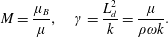 $$\begin{eqnarray}M=\frac{\unicode[STIX]{x1D707}_{B}}{\unicode[STIX]{x1D707}},\quad \unicode[STIX]{x1D6FE}=\frac{L_{d}^{2}}{k}=\frac{\unicode[STIX]{x1D707}}{\unicode[STIX]{x1D70C}\unicode[STIX]{x1D714}k}.\end{eqnarray}$$
The solution of this pair of equations is (cf. (2.8))
 $$\begin{eqnarray}\displaystyle & \displaystyle u=U_{3}\exp \left(-\text{i}^{1/2}y\right),\quad y>0, & \displaystyle\end{eqnarray}$$
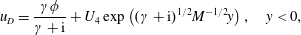 $$\begin{eqnarray}\displaystyle & \displaystyle u_{D}=\frac{\unicode[STIX]{x1D6FE}\unicode[STIX]{x1D719}}{\unicode[STIX]{x1D6FE}+\text{i}}+U_{4}\exp \left((\unicode[STIX]{x1D6FE}+\text{i})^{1/2}M^{-1/2}y\right),\quad y<0, & \displaystyle\end{eqnarray}$$
 $U_{3}$
,
$U_{3}$
,
 $U_{4}$
are constants that will be found when we apply the boundary conditions on
$U_{4}$
are constants that will be found when we apply the boundary conditions on
 $y=0$
. We see in (A 7b
) that higher shear stresses when
$y=0$
. We see in (A 7b
) that higher shear stresses when
 $M>1$
lead to a slower spatial rate of decay of the velocity
$M>1$
lead to a slower spatial rate of decay of the velocity
 $u_{D}$
as
$u_{D}$
as
 $y\rightarrow -\infty$
.
$y\rightarrow -\infty$
.
After non-dimensionalization, the boundary conditions (A 3) and (A 4) become
 $$\begin{eqnarray}u-\frac{u_{D}}{\unicode[STIX]{x1D6FC}}=\unicode[STIX]{x1D706}\frac{\unicode[STIX]{x2202}u}{\unicode[STIX]{x2202}y}+\left(1-\frac{\unicode[STIX]{x1D719}}{\unicode[STIX]{x1D6FC}}\right),\quad \frac{\unicode[STIX]{x2202}u}{\unicode[STIX]{x2202}y}-M\frac{\unicode[STIX]{x2202}u_{D}}{\unicode[STIX]{x2202}y}=\unicode[STIX]{x1D6FD}u-\unicode[STIX]{x1D6FD},\quad y=0,\end{eqnarray}$$
where
 $\tilde{\unicode[STIX]{x1D6FD}}=\unicode[STIX]{x1D6FD}\unicode[STIX]{x1D707}/L_{d}=\unicode[STIX]{x1D6FD}(\unicode[STIX]{x1D70C}\unicode[STIX]{x1D714}\unicode[STIX]{x1D707})^{1/2}$
and
$\tilde{\unicode[STIX]{x1D6FD}}=\unicode[STIX]{x1D6FD}\unicode[STIX]{x1D707}/L_{d}=\unicode[STIX]{x1D6FD}(\unicode[STIX]{x1D70C}\unicode[STIX]{x1D714}\unicode[STIX]{x1D707})^{1/2}$
and
 $\tilde{\unicode[STIX]{x1D706}}=L_{d}\unicode[STIX]{x1D706}=\unicode[STIX]{x1D706}(\unicode[STIX]{x1D707}/\unicode[STIX]{x1D70C}\unicode[STIX]{x1D714})^{1/2}$
. These boundary conditions lead to (cf. (2.9))
$\tilde{\unicode[STIX]{x1D706}}=L_{d}\unicode[STIX]{x1D706}=\unicode[STIX]{x1D706}(\unicode[STIX]{x1D707}/\unicode[STIX]{x1D70C}\unicode[STIX]{x1D714})^{1/2}$
. These boundary conditions lead to (cf. (2.9))
 $$\begin{eqnarray}U_{3}=\frac{\unicode[STIX]{x1D6FD}+M^{1/2}(\unicode[STIX]{x1D6FE}+\text{i})^{1/2}[\unicode[STIX]{x1D6FC}-\unicode[STIX]{x1D719}\text{i}/(\unicode[STIX]{x1D6FE}+\text{i})]}{\unicode[STIX]{x1D6FD}+\text{i}^{1/2}+\unicode[STIX]{x1D6FC}M^{1/2}(\unicode[STIX]{x1D6FE}+\text{i})^{1/2}(1+\text{i}^{1/2}\unicode[STIX]{x1D706})}\end{eqnarray}$$
and
 $$\begin{eqnarray}U_{4}=\frac{\unicode[STIX]{x1D6FD}(1+\text{i}^{1/2}\unicode[STIX]{x1D706})\unicode[STIX]{x1D6FC}-(\unicode[STIX]{x1D6FD}+\text{i}^{1/2})[\unicode[STIX]{x1D6FC}-\unicode[STIX]{x1D719}\text{i}/(\unicode[STIX]{x1D6FE}+\text{i})]}{\unicode[STIX]{x1D6FD}+\text{i}^{1/2}+\unicode[STIX]{x1D6FC}M^{1/2}(\unicode[STIX]{x1D6FE}+\text{i})^{1/2}(1+\text{i}^{1/2}\unicode[STIX]{x1D706})}.\end{eqnarray}$$
We note that when
 $\unicode[STIX]{x1D719}=1$
,
$\unicode[STIX]{x1D719}=1$
,
 $\unicode[STIX]{x1D6FC}=1$
,
$\unicode[STIX]{x1D6FC}=1$
,
 $M=1$
,
$M=1$
,
 $\unicode[STIX]{x1D6FD}=0$
,
$\unicode[STIX]{x1D6FD}=0$
,
 $\unicode[STIX]{x1D706}=0$
we recover the analysis of § 2, i.e.
$\unicode[STIX]{x1D706}=0$
we recover the analysis of § 2, i.e.
 $U_{3}=U_{1}$
,
$U_{3}=U_{1}$
,
 $U_{4}=U_{2}$
.
$U_{4}=U_{2}$
.
The force that the solid exerts on the fluid due to relative motion is
 $\unicode[STIX]{x1D707}(\unicode[STIX]{x1D719}\tilde{u} _{s}-\tilde{u} _{D})/k$
, and so the dimensionless rate of working of the solid as it oscillates is now (cf. (2.10))
$\unicode[STIX]{x1D707}(\unicode[STIX]{x1D719}\tilde{u} _{s}-\tilde{u} _{D})/k$
, and so the dimensionless rate of working of the solid as it oscillates is now (cf. (2.10))
 $$\begin{eqnarray}W(y,t)=\unicode[STIX]{x1D6FE}\text{Re}\left\{\left[\unicode[STIX]{x1D719}-\frac{\unicode[STIX]{x1D6FE}\unicode[STIX]{x1D719}}{\unicode[STIX]{x1D6FE}+\text{i}}-U_{4}\exp \left((\unicode[STIX]{x1D6FE}+\text{i})^{1/2}M^{-1/2}y\right)\right]\text{e}^{\text{i}t}\right\}\text{Re}\left\{\text{e}^{\text{i}t}\right\}.\end{eqnarray}$$
The rest of the analysis continues along the same lines as in § 2. We see that the use of these predictions to interpret experiments designed to investigate the Brinkman viscosity
 $\unicode[STIX]{x1D707}_{B}$
would involve a simultaneous investigation of the boundary conditions at the interface
$\unicode[STIX]{x1D707}_{B}$
would involve a simultaneous investigation of the boundary conditions at the interface
 $y=0$
.
$y=0$
.


 Open access