2.1. Basic equation of motion for 3-D and 2-D hydrodynamics

This paper is based on the Wyld diagrammatic technique for hydrodynamic turbulence (Wyld Reference Wyld1961) generalized by Martin, Siggia & Rose (Reference Martin, Siggia and Rose1973) and by Zakharov & L'vov (Reference Zakharov and L'vov1975). Its detailed review is available in L'vov & Procaccia (Reference L'vov and Procaccia1995). Generally speaking, the proposed technique can be applied straightforwardly to any integer dimensions, including either 2-D or 3-D turbulence that differs in the analytical form of the Navier–Stokes equations, as well as to other problems, for example, passive scalar. Its application for non-integer dimensions is more tricky and requires understanding how to perform integrations in non-integer dimensions; see e.g. L'vov et al. (Reference L'vov, Pomyalov and Procaccia2002).

In the 3-D case, the Euler equations for the velocity $\boldsymbol{v}(\boldsymbol{r},t)$ of an incompressible fluid with density $\rho =1$ have the well-known form (Landau & Lifshitz Reference Landau and Lifshitz2013)

(2.1a) \begin{equation} \frac{\partial \boldsymbol{v}(\boldsymbol{r},t)}{\partial t} + (\boldsymbol{v} \boldsymbol{\cdot} \boldsymbol{\nabla})\boldsymbol{v} + \boldsymbol{\nabla} p= 0, \quad \boldsymbol{\nabla} \boldsymbol{\cdot} \boldsymbol{v}= 0. \end{equation}

In the $(\boldsymbol{k}, t)$ representation for the vector components $u^\alpha (\boldsymbol{k}, t)$, (2.1a) can be rewritten as

(2.1b) \begin{equation} \frac{\partial v^\alpha (\boldsymbol{k}, t)}{\partial t}= \frac12 \int \frac{{\rm d}^3 k_1\, {\rm d}^3 k_2}{ (2{\rm \pi})^2}\,\delta (\boldsymbol{\kappa}+\boldsymbol{\kappa}_1+\boldsymbol{\kappa}_2)\,\varGamma_{k12}^{\alpha\beta\gamma}\, u^{* \,\beta }_{\kappa_1}\,u^{*\,\gamma}_{\kappa_2}; \end{equation}

see e.g. L'vov & Procaccia (Reference L'vov and Procaccia1995). Here, $\varGamma _{k12}^{\alpha \beta \gamma }$ is the interaction amplitude

(2.1c)\begin{equation} \varGamma_{k12}^{\alpha\beta\gamma}={\rm i}\sum_{\alpha'} \left( \delta_{\alpha \alpha'} -\frac{k^\alpha k^{\alpha'}}{k^2} \right)( k^{\beta}\delta_{\alpha'\gamma}+ k^\gamma \delta_{\alpha'\beta}), \end{equation}

where $\delta _{\alpha \beta }$ is $1$ if $\alpha =\beta$, and vanishes otherwise. Euler equation (2.1a) preserves the total energy of the flow

(2.1d)\begin{equation} \mathcal{E} = \int |\boldsymbol{v}(\boldsymbol{r},t)|^2 \,{\rm d}^3 r= \int |\boldsymbol{u}(\boldsymbol{k},t)|^2\,\frac{{\rm d}^3 k}{(2{\rm \pi})^3}. \end{equation}

Therefore $\varGamma _{k12}^{\alpha \beta \gamma }$ satisfies Jacobi identity

(2.1e)\begin{equation} \varGamma_{k12}^{\alpha\beta\gamma}+\varGamma_{2k1}^{\gamma\alpha\beta}+ \varGamma_{12k} ^{\beta\gamma\alpha}=0 \end{equation}

on the surface $\boldsymbol{k}+ \boldsymbol{k}_1+ \boldsymbol{k}_2=0$.

The basic equations of motion for 2-D turbulence have a structure similar to the 3-D case (2.1). The 2-D turbulence may be represented as a scalar equation for the vorticity, which simplifies analytical expressions. Therefore, for the transparency of the presentation, we illustrate our formalism for the 2-D turbulence. In the present work, following L'vov et al. (Reference L'vov, Pomyalov and Procaccia2002), we consider the Euler equation for the vorticity equation in 2-D:

(2.2)\begin{equation} \partial {\omega}/ \partial t+ ({\boldsymbol{u}}\boldsymbol{\cdot} {\boldsymbol \nabla}) \omega=0. \end{equation}

The velocity and vorticity of a 2-D flow may be derived from the stream function $\psi ({\boldsymbol{x}},t)$ as ${\boldsymbol{u}} ({\boldsymbol{x}},t)=-{\boldsymbol \nabla } \times \hat {\boldsymbol{z}}\, \psi (\hat {\boldsymbol{x}},t)$ and $\omega ({\boldsymbol{x}},t) = -\nabla ^2 \psi ({\boldsymbol{x}},t)$, where $\hat {\boldsymbol{z}}$ is a unit vector orthogonal to the $\hat {\boldsymbol{x}}$-plane, and $\nabla ^2$ is the Laplacian operator in the plane. In the $\boldsymbol{k}$ representation, $a(\boldsymbol{k},t)\equiv k\int {\rm d}{\boldsymbol{R}} \exp [-{\rm i}({ \boldsymbol{R}}\boldsymbol {\cdot }{\kappa } )]\,{\psi }(\boldsymbol{R},t)$. The Fourier transforms of and are denoted as ${\boldsymbol{v}}(\kappa,t)$ and ${ \varOmega }(\kappa,t)$, respectively. These Fourier transforms are expressed in terms $a(\kappa,t)$, re-designated for the shortness as $a_{\boldsymbol{k}}$: $\boldsymbol{v}(\kappa,t)={\rm i}(\hat {{\boldsymbol z}}\times \hat {\kappa }) a_\kappa$ and $\varOmega (\kappa,t)= -k a_\kappa$, where $\hat {\kappa } =\kappa /k$. Now, by (2.2),

(2.3) \begin{equation} \left.\begin{gathered} \frac{\partial a_\kappa }{ \partial t} = \int \frac{{\rm d}^2 k_1 \,{\rm d}^2 k_2}{2\times2{\rm \pi}}\,\delta (\boldsymbol{\kappa}+\boldsymbol{\kappa}_1+\boldsymbol{\kappa}_2)\,V_{k12} a^*_{\kappa_1}a^*_{\kappa_2},\\ V_{k12} = \frac{S_{k12}(k_2^2-k_1^2)}{2 kk_1k_2},\quad S_{k12} \equiv2 k_1 k_2 \sin \varphi_{12} , \\ S_{k12} =S_{2k1}=S_{12k}={-} S_{k21}={-} S_{1k2}={-} S_{21k},\\ |S_{k12}| = \sqrt{2(k^2k_1^2+k_1^2k_2^2+k_2^2k^2) -k^4-k_1^4-k_2^4} . \end{gathered}\right\} \end{equation}

Here, the interaction amplitude (or ‘vertex’) $V_{k12}$ is expressed via $S_{k12}$, where $|S_{k12}|/4$ is the area of the triangle formed by the vectors $\boldsymbol{\kappa}$, $\boldsymbol{\kappa}_1$ and $\boldsymbol{\kappa}_2$. Also, $\varphi _{12}=\varphi _1-\varphi _2$, with $\varphi _k$, $\varphi _1$ and $\varphi _2$ the angles in the triangular plane between the $x_1$-axis and the vectors $\kappa$, $\kappa _1$ and $\kappa _2$, respectively. The vertex $V_{k12}$ satisfies two Jacobi identities:

(2.4a,b)\begin{equation} (V_{k12}+V_{2k1}+V_{12k})=0, \quad (k^2V_{k12}+k_2^2V_{2k1}+k_1^2V_{12k})=0. \end{equation}

These two identities ensure the conservation of energy $\mathcal {E}$ in the inviscid forceless limit and the enstrophy $\mathcal {H}$ given by

(2.5a,b)\begin{equation} \mathcal{E}\equiv \int |a_k|^2\,\frac{{\rm d} ^2 k}{(2{\rm \pi})^2}, \quad \mathcal{H}\equiv \int k^2 |a_k|^2\,\frac{{\rm d} ^2 k}{(2{\rm \pi})^2}. \end{equation}

Equation (2.3) describes the 2-D hydrodynamic turbulence. One sees that it has the same form as the 3-D (2.1), but without additional vector indices. Therefore, the results of this paper are applicable for both 2-D and 3-D turbulence. The concrete conclusions of our paper depend on the presence of the Jacobi identity for the symmetry of the matrix element. The 2-D turbulence has two quadratic integrals of motion (energy and enstrophy) and two Jacobi identities (2.4a,b) that reflect this fact. The 3-D turbulence has one integral of motion and just one Jacobi identity (2.1e). As shown e.g. by Kraichnan & Montgometry (Reference Kraichnan and Montgometry1980), the physical properties of these two systems are different, yet they are described by the same technique and same triangular re-summation. To simplify our presentation, we focus in the paper on the 2-D turbulence.

Following Wyld (Reference Wyld1961), we divide the world into the system under consideration and the thermostat. The action of the thermostat on the system is modelled by random noise $f(\boldsymbol{k},t)$ and damping $\gamma _0(k)$. Then we replace $\partial a_\kappa / \partial t$ of (2.3) with $[\partial / \partial t+ \gamma _0(\boldsymbol{k}) ]a_\kappa - f(\boldsymbol{k},t)$, so that we obtain instead

(2.6)\begin{equation} \left[\frac{\partial }{\partial t}+ \gamma_0(\boldsymbol{k}) \right]a_\kappa =\int \frac{{\rm d}^2 k_1 \,{\rm d}^2 k_2}{2\times2{\rm \pi}}\,\delta (\boldsymbol{\kappa}+\boldsymbol{\kappa}_1+\boldsymbol{\kappa}_2)\,V_{k12} a^*_{\kappa_1}a^*_{\kappa_2}+f(\boldsymbol{k},t), \end{equation}

where the average statistics of the noise $f(\boldsymbol{k},t)$ is assumed to satisfy $\langle\,f(\boldsymbol{k},t)\, f(\boldsymbol{k}',t') \rangle \propto$ $T\,\gamma _0(\boldsymbol{k},t)\,\delta (\boldsymbol{k}- \boldsymbol{k}')\,\delta (t-t')$. Here, $\langle \cdot \rangle$ denotes an average with respect to the thermo- dynamic equilibrium ensemble with temperature $T$. The presence of the thermostat force and the damping allows (2.6) to have non-trivial solutions. After the Dyson–Wyld line-re-summation, described below, we will disconnect our system from the thermostat by taking the limit $\gamma _0(\boldsymbol{k})\to 0$. It was shown by Wyld (Reference Wyld1961) and Zakharov, L'vov & Starobinets (Reference Zakharov, L'vov and Starobinets1975) that the result is independent of the thermostat parameters.

After the Fourier transformation with respect to time $t$, (2.6) in the ${\boldsymbol q}=(\boldsymbol{k}, \omega )$ representation becomes

(2.7)\begin{equation} a_{\boldsymbol q}=\,{}^{0}\!\mathcal{G}_{\boldsymbol q}\left[ \frac12\int \frac{{\rm d} \boldsymbol{q}_1 \,{\rm d} \boldsymbol{q}_2}{ (2{\rm \pi})^{d+1}}\,\delta^{d+1}_{q12} V_{k 1 2} a^*_1 a^*_2 + f_{\boldsymbol q}\right], \quad {}^{0}\!\mathcal{G}_{\boldsymbol{q}}= {\rm i}/[\omega+{\rm i}\,\gamma_0(\boldsymbol{k})]. \end{equation}

Here, $^{0}\!\mathcal {G}_{\boldsymbol{q}}$ is the bare Green's function, ${\rm d} \boldsymbol{q}_j \equiv {\rm d}^2 k_j \,{\rm d}\omega _j$, and $V_{\boldsymbol{k} \boldsymbol{1} \boldsymbol{2}} \equiv V(\boldsymbol{k} ,\boldsymbol{k}_1 ,\boldsymbol{k}_2)$ is the interaction matrix element describing the strength of interactions between wavenumbers $\boldsymbol{k}$, $\boldsymbol{k}_1$ and $\boldsymbol{k}_2$.

2.2. Iterative expansion for field variables $a$$_{q}$

Introducing the zero-order solution of this equation, $^{0}\!a_{\boldsymbol{q}} \equiv {}^{0}\!\mathcal {G}_{\boldsymbol{q}}\, f_{\boldsymbol q}$, we can get its iterative solution as a formal infinite series with respect to powers of $^{0}\!a_{\boldsymbol{q}}$: , where

(2.8a)

(2.8b)

(2.8c)

(2.8d)

(2.8e)

(2.8f)

(2.8g)

Here, $\boldsymbol{q}_1+\boldsymbol{q}_2+\boldsymbol{q}_3=0$, $\mathcal {G}_j \equiv \mathcal {G}(\boldsymbol{q}_j)$ and ${\mathcal {F}}_j \equiv \mathcal {F}(\boldsymbol{q}_j)$, and a subscript with an overline denotes the negative of the corresponding wave vector, e.g. $\bar {j}=-\boldsymbol{q}_j$. Here, and are the zeroth-, first-, second-, third- and fourth-order iterations in the powers of interaction matrix element $V$; the number to the left of $a$ denotes the order of the iteration. For the third and fourth orders, there are contributions of different topologies, so the letters ‘a’, ‘b’ and ‘c’ are used to differentiate between them.

Using graphical notation shown in figure 1, we can present each term in this series in a graphical form as a ‘tree’ diagram, as shown in figure 2. In these diagrams, the Green's function ${}^{0}\!G_{\boldsymbol{q}}$ is shown as a thin wavy–straight line, the ${}^0\!a_{\boldsymbol{q}}$ is shown as a short thin wavy line. The ${}^0\!a_{\boldsymbol{q}}$ are shown as thin wavy lines that are connected by vertex $V_{123}$ shown as a fat dot ‘$\bullet$’. The vertex has one straight tail, belonging to ${}^{0}\!G_{\boldsymbol{q}_1}$ and two wavy tails, belonging to ${}^0\!a_{\boldsymbol{q}_2}$ and ${}^0\!a_{\boldsymbol{q}_3}$. The key realization that gives birth to the diagrammatic technique is that instead of deriving (2.8), we could have had drawn all possible topologically different trees, without deriving (2.8) analytically first.

Figure 1. Graphical notation for the line re-summed Wyld's diagrammatic expansion. A short wavy line stands for the canonical variable $a_{\boldsymbol{q}} =a(\boldsymbol{k},\omega )$. A straight line stands for the random force field $f(\boldsymbol{r},t)$ that appears in (2.6). The Green's function $\mathcal {G}(\boldsymbol{k},\omega )$, which is the response in the vorticity to some force, is made up of a short wavy line and a short straight line. A long wavy line represents double correlation functions $\mathcal {F}(\boldsymbol{k}, \omega )$ of the velocities. The vertex $V_{123}$ (see (2.6)) is a fat dot with three tails. One straight tail belongs to the Green's function, and two wavy tails represent velocities. A triangle with three wavy lines represents simultaneous three-point correlators of the first order ${}^3\! \mathcal {F}^{{{I}}}_{123}$ (thin triangle) and of the third order ${}^3\! \mathcal {F}^{{{III}}}_{123}$ (thick triangle), and a fully dressed three-point correlator (in all orders) ${}^3\! \mathcal {F} _{123}$ (red filled triangle).

Figure 2. Graphical representation of the iterative expansion of $a_{\boldsymbol{q}}$, given by (2.8). We have reserved indices 1, 2, 3 and 4 ($\boldsymbol{q}_1$, $\boldsymbol{q}_2$, $\boldsymbol{q}_3$ and $\boldsymbol{q}_4$) for the arguments of the correlation functions. Therefore, we supplied wavy tails of the trees for ${}^n\! a_j$ with indices $j=5,6,\ldots$. Here, the left superscript ${}^n$ denotes the iteration order (the number of the vertices in trees).

Analysing (2.8) and figure 2 with the trees, we see that the trees with the symmetrical elements have a numerical prefactor that is given by $1/N$, where $N$ is the number of elements of the symmetry group of a diagram. This is a constructive demonstration of the ${1}/{N}$ symmetry rule for the trees. We will see this rule again when we consider diagrams for the correlation function. The symmetry factor appears as a consequence of the ${\boldsymbol{k}_1}\leftrightarrow {\boldsymbol{k}_2}$ symmetry and factor $1/2$ in the equation of motion (2.6). The rigorous proof of the ${1}/{N}$ symmetry rule is beyond the scope of the present paper. The ${1}/{N}$ symmetry rule will play a crucial role below, as it will lead to the natural grouping of the diagrams into triads. It would be much harder to see this rule by looking at analytical expressions alone.

The next important advantage of a diagrammatic technique is that from topological properties of the diagrams, one can make conclusions about the corresponding analytical expression without detailed analysis, and even perform a partial re-summation of diagrams with particular topological properties. This observation leads to the Dyson–Wyld line re-summation of reducible diagrams. A reducible diagram is one that contain fragments that can be disconnected from the rest of the diagram by cutting two lines. If these cut lines are wavy and straight ones, then the infinite sum of the corresponding fragments becomes ‘dressed’, Green's function $\mathcal {G}_{\boldsymbol{q}}$, defined as $\langle \partial a_{\boldsymbol q}/ \partial f_{\boldsymbol{q}'}\rangle =(2{\rm \pi} )^{d+1} \delta ^{d+1} ({\boldsymbol q}-\boldsymbol{q}')\,\mathcal {G}_{\boldsymbol{q}}$. This Green's function can be presented as (see e.g. Wyld Reference Wyld1961; Zakharov, L'vov & Musher Reference Zakharov, L'vov and Musher1972; Martin et al. Reference Martin, Siggia and Rose1973)

(2.9a,b)\begin{equation} \mathcal{G}_{\boldsymbol{q}}= {\rm i} / [\omega + {\rm i}\,\gamma_0(\boldsymbol{k})-\varSigma_{\boldsymbol{q}} ], \quad -{\rm Im}[\varSigma_{\boldsymbol q}] =\varGamma_{\boldsymbol{q}}=k^2\, \nu_{{turb}}(k), \end{equation}

where the ‘mass operator’ $\varSigma _{\boldsymbol{q}}$ is an infinite sum of diagrams that begin and end with a vertex, and determines the ‘turbulent’ dissipation $\nu _{{turb}}$. In the case where cut lines in the reducible diagram are two wavy lines, the infinite sum corresponds to the ‘dressed’ double correlator ${\mathcal {F}}_{\boldsymbol{q}}$, defined in the next subsection by (2.10a), shown in diagrams as long thick wavy lines.

After performing the Dyson–Wyld line re-summation, in the expansion (2.8) it is possible to replace the bare Green's functions ${}^{0}\!\mathcal {G}_{\boldsymbol{q}}$ by their dressed counterparts $\mathcal {G}_{\boldsymbol{q}}$. Furthermore, it is possible to replace the bare field ${}^{0}\!a_{\boldsymbol{q}}$ by the dressed field $a_{\boldsymbol{q}}$. Such modification presents the essence of ‘dressing’, i.e. moving terms from higher orders of the perturbation theory to lower orders, and combining them into the ‘dressed’ objects. The ‘dressed’ version of (2.8) will be used in the rest of the paper.

2.3. Diagrammatic expansion of correlation functions

2.3.1. Definitions and procedure

We define the two-, three-, four- and $n$-point correlators in $\boldsymbol{q}=(\boldsymbol{k},\omega )$ space as

(2.10a)\begin{gather} \left.\begin{gathered} (2{\rm \pi})^{d+1}\delta( {\boldsymbol{q}_1}+{\boldsymbol{q}_2}) \,{}^{2}\! {\mathcal{F}} ({\boldsymbol{q}_1},{\boldsymbol{q}_2}) = \frac{\langle a_{\boldsymbol{q}_1} a_{\boldsymbol{q}_2}\rangle}{ 2!} , \\ (2{\rm \pi} )^{d+1}\delta( {\boldsymbol{q}_1}+{\boldsymbol{q}_2}+{\boldsymbol{q}_3}) \, {}^{3}\! {\mathcal{F}}({\boldsymbol{q}_1},{\boldsymbol{q}_2},{\boldsymbol{q}_3}) = \frac{\langle a_{\boldsymbol{q}_1} a_{\boldsymbol{q}_2}a_{\boldsymbol{q}_3}\rangle}{ 3!}, \end{gathered}\right\} \end{gather}

(2.10b)\begin{gather} (2{\rm \pi})^{d+1}\delta( {\boldsymbol{q}_1}+{\boldsymbol{q}_2}+{\boldsymbol{q}_3}+{\boldsymbol{q}_4}) \, {}^ {4}\! {\mathcal{F}}({\boldsymbol{q}_1},{\boldsymbol{q}_2},{\boldsymbol{q}_3},{\boldsymbol{q}_4}) = \langle a_{\boldsymbol{q}_1} a_{\boldsymbol{q}_2}a_{\boldsymbol{q}_3} a_{\boldsymbol{q}_4}\rangle/(4!), \end{gather}

(2.10c)\begin{gather} \left.\begin{gathered} (2{\rm \pi})^{d+1}\delta\left(\sum_{j=1}^n {\boldsymbol{q}_j}\right)\, {}^{n}\! {\mathcal{F}} ({\boldsymbol{q}_1},\ldots, {\boldsymbol{q}_n}) \equiv {\left\langle \prod_{j=1}^n a_{\boldsymbol{q}_j}\right\rangle}/ {( n!)} ,\quad n = 2,3,\ldots,\\ ^{2}\!\mathcal{F}(\boldsymbol{q}) \equiv {}^{2}\!\mathcal{F}(\boldsymbol{q}, -\boldsymbol{q}). \end{gathered}\right\} \end{gather}

Here, $d$ is the dimension of space. In the case of 2-D turbulence, $d=2$. We have included prefactor $1/ n!$ in the definition (2.10) of $n$-point correlation function ${}^{n}\!\mathcal {F}$. Note that $n!$ is the number of elements of the symmetry group of a correlator, which is equal to the number of permutations in the definition of ${}^{n}\!\mathcal {F}$ in the definition (2.10a). This is precisely the choice that ensures the applicability of our $1/N$ symmetry rule for the correlation functions. As we will see below, this particular choice simplifies the appearance of final expressions for ${}^{n}\!\mathcal {F}$. Notice that the notation ${}^{2}\!\mathcal {F} ({\boldsymbol{q}},{\boldsymbol{q}'})$ involves two arguments, while actually, it depends on only one argument, say $\boldsymbol{q}$. Therefore, in (2.10c), we define it in the more traditional way.

Diagrammatic presentations of ${}^{2}\!\mathcal{F}$, ${}^{3}\!\mathcal {F}$ and ${}^{4}\!\mathcal {F}$ can be obtained by gluing together two, three and four trees. The gluing is a graphical representation of the averaging over the ensemble of the random force. On the corresponding diagrams of two glued trees, the dashed line crossing out the double correlator is the point where the ‘branches’ of two trees were ‘glued’ to form a double correlator. The number of possible combinations of the glued trees will be of crucial importance in further investigation of the diagrammatic series.

For the Gaussian process, the high-order correlation functions can be presented as a product of all possible second-order correlators. Specifically, this means that

(2.11a–c)\begin{equation} \langle a_k^* a^*_l a_p a_n \rangle = \mathcal{F} _k \mathcal{F}_l(\delta^k_p\delta ^l_n + \delta^k_n\delta ^l_p),\quad \langle a_k^* a_l a_p a_n\rangle =0 , \quad \langle a_k a_l a_p a_n\rangle = 0. \end{equation}

In this paper, the $n$-point correlators ${}^{n}\!\mathcal {F}$ also will be classified by the number $m$ of interacting vortices in the diagrams, shown as superscript on the right: ${}^{n}\!\mathcal {F}^m$. Thus the lowest and next to lowest diagrams for ${}^{3}\!\mathcal{F}$ and ${}^{4}\!\mathcal {F}$ are denoted as ${}^{3}\!\mathcal {F}^{{{I}}}$, ${}^{3}\!{\mathcal {F}}^{{{III}}}$ and ${}^{4}\!\mathcal {F}^{{{II}}}$, ${}^{4}\!\mathcal {F}^{{{IV}}}$. We will see that the numerical prefactors before the diagrams play a critical role in the triangular re-summation.

2.3.3. Third-order correlator ${}^{3}\!{\mathcal {F}}^{{{I}}}$ and ${}^{3}\!\mathcal {F}^{{{III}}}$

We consider first-order diagrams for triple correlator ${}^{3}\mathcal{F}^1$. Its first representative ${}^{3}\!{\mathcal {F}}_{123}^{1A}$ is shown in figure 3(a) as a diagram ${}^{1}\!\!\mathcal {A}_{1,23}$. From definition (2.10a), one gets

(2.12a)\begin{equation} \left.\begin{gathered} (2{\rm \pi})^{d+1}\delta_{123} \,{}^3\! \mathcal{F}_{123}^{1A} = \underset{123}{\boldsymbol P}{}^1\!\!\mathcal{A}_{1,23}, \quad (2{\rm \pi})^{d+1}\delta_{123} \, {}^1\!\!\mathcal{A}_{1,23} = \tfrac{1}{2} \langle a_1^{ 1 } a_2 a_3 \rangle , \\ \delta_{123} \equiv \delta(\boldsymbol{q}_1+\boldsymbol{q}_2+\boldsymbol{q}_3). \end{gathered}\right\} \end{equation}

Here, $\underset {123}{\boldsymbol P}$ is the permutation operator that, when acting on the function, produces a sum of all possible permutations of its indices divided by the number of all possible permutations of the indices. For example, $\underset {123}{\boldsymbol P}{\mathcal {A}}_{1,23} \equiv \frac {1}{3!}( {\mathcal {A}}_{1,23}+{\mathcal {A}}_{1,32}+{\mathcal {A}}_{2,13} + {\mathcal {A}}_{2,31}+{\mathcal {A}}_{3,12}+{\mathcal {A}}_{3,21})$. Substituting ${}^1\!a_1$ from (2.8a) into ${}^1\!\!\mathcal {A}_{1,23}$, one gets . Hereafter, we colour in parts originating from the tree in (A16a). We now average the resulting expression using the pairing rule (2.11a–c), which corresponds to gluing together the trees of ${}^1\!a_{\boldsymbol{q}}$ and $a_{\boldsymbol{q}}$. The result is pairs and $\overbrace {a_2\,a_3}$ that give uncoupled contributions (each of them is equal to zero). Two equivalent ways to pair and (denoted for the brevity as and , or even more briefly as ) result in

(2.12b)

Graphically, this result is shown in figure 3(a). We preserve the notation ${}^n\!\!\mathcal {A}_{1,2\ldots }$ for all diagrams of $n$th order in vertices $V$ with one leg denoting the Green's function $\mathcal {G}_1$ and any number of wavy tails denoting ${\mathcal {F}}_j$. Here and in the rest of the paper, we separate by a comma the indices in the correlators corresponding to the Green's functions from those corresponding to the double correlators.

Figure 3. The lowest-order contributions to (a) the three-point correlator ${}^{3}\!\mathcal {F}^{1A}_{123}$ and (b,c) the four-point correlator ${}^{3}\!\mathcal {F}^{2A}_{1234}$ and ${}^{3}\!\mathcal {F}^{2B}_{1234}$ as a result of gluing of three and four trees, separated by $\parallel$. All diagrams include prefactors. The operator $\boldsymbol{P}$ is not shown explicitly on this and subsequent diagrams, but its presence is implied.

For third-order diagrams for triple correlator ${}^{3}\mathcal{F}^3$, we compute the three-point correlator in the third order in the interaction vertex. As we will show below, this object plays a key role in the statistical properties of hydrodynamic turbulence. This object appears as a result of gluing together three trees and leads to the diagrams that are triangular in shape. To calculate ${}^{3}\! \mathcal {F}^{3}$, we use (2.10a) and collect all terms $\propto V^3$:

(2.13) \begin{equation} \left.\begin{gathered} (2{\rm \pi})^{d+1} {\delta^{d+1}_{123}}\, {}^3 \! \mathcal{F}_{123}^{(3)}= \underset{123}{\boldsymbol P}[ {}^{3a}\!\!{\mathcal{A}}_{1,23}+ {}^{3b}\!\!{\mathcal{A}}_{1,23} + {}^3\! {\mathcal{B}}_{12,3} + {}^3\! {\mathcal{C}}_{123} ],\\ {}^{3a}\!\!{\mathcal{A}}_{1,23}= \langle {}^{3a}\!a_1 a_2 a_3 \rangle / 2, \quad {}^{3b}\!\!{\mathcal{A}}_{1,23}= \langle \, {}^{3b}\!a_1 a_2 a_3\rangle / 2 , \\ {}^3\! {\mathcal{B}}_{12,3}=\langle a_1^{2} a_2^{1} a_3 \rangle , \quad {}^3\!{\mathcal{C}}_{123}= {\langle a_1^ 1 a_2^ 1 a_3^ 1 \rangle } / {3!}. \end{gathered}\right\} \end{equation}

These terms are computed in § A.1, and the results are given by

(2.14a)$$\begin{gather} {}^{3a}\!\!{\mathcal{A}}_{1,23} = \mathcal{G}_1 {\mathcal{F}}_2 {\mathcal{F}}_3 \int \frac{{\rm d} \boldsymbol{q}_4}{(2{\rm \pi})^{d+1}}\,V_{14{\overline{1+4}}}V_{{\bar{4}}(4-2)2} V_{(2-4)3(1+4)} \mathcal{G}_4^* \mathcal{G}_{2-4} {\mathcal{F}}_{1+4} , \end{gather}$$

(2.14b)$$\begin{gather}{}^{3b}\!\!{\mathcal{A}}_{1,23}=\frac12 \mathcal{G}_1 {\mathcal{F}}_2 {\mathcal{F}}_3 \int \frac{{\rm d} \boldsymbol{q}_4}{(2{\rm \pi})^{d+1}}\,\mathcal{G}^*_4 {\mathcal{F}}_{2-4}\mathcal{G}_{1+4} V_{14\overline{(1+4)}} V_{{\bar{4}}(4-2)2} V_{(4+1)3(2-4)} , \end{gather}$$

(2.14c)$$\begin{gather}{}^3\!{\mathcal{B}}_{12,3}=\mathcal{G}_1 \mathcal{G}_2 {\mathcal{F}}_3 {{\int}}\frac{{\rm d}\boldsymbol{q}_4}{(2{\rm \pi})^{d+1}}\,{\mathcal{F}}_4 {\mathcal{F}}_{4-2} \mathcal{G}_{1+4} V_{14\overline{(1+4)}}V_{2{\bar{4}(4-2)}}V_{(4+1)3(2-4)} , \end{gather}$$

(2.14d)$$\begin{gather}{}^3\!{\mathcal{C}}_{123}= \frac{1}{6}\mathcal{G}_1 \mathcal{G}_2 \mathcal{G}_3 {{\int}} \frac{{\rm d}\boldsymbol{q}_4}{(2{\rm \pi})^{d+1}}\,{\mathcal{F}}_4 {\mathcal{F}}_{4-2} {\mathcal{F}}_{1+4} V_{14\overline{(1+4)}} V_{2{\bar{4}}(4-2)}V_{3(1+4)(2-4)} . \end{gather}$$

Recall that an overline over indices indicates the negative of the corresponding wave vector, and the sums of indices imply the sum of corresponding wavenumbers, e.g. $V_{14\overline {(1+4)}}\equiv V_{k_1, k_4, -k_1-k_4}$. The corresponding diagrams are shown in figures 4(a–d).

Figure 4. Triangular diagrams for the next-lowest third-order triple correlation function as a result of gluing three trees, separated by $\parallel$. Diagrams with one, two and three Green's function in the legs are denoted as $\mathcal {A}$, $\mathcal {B}$ and $\mathcal {C}$. All diagrams include prefactors according to the $1/N$ symmetry rule.

2.3.4. Four-point correlation function

Second-order diagrams for $^{4}\mathcal {F}^{(2)}$ are proportional to the product of two vertices $V$. They originates from ten terms, which we divide into two groups ${}^{2}\!\!\mathcal {A}_{1,234}$ with one and two $G$-tails involving Green's functions. Hereafter, we preserve the notation ${}^n\!{\mathcal {B}}_{12,\ldots }$ for all diagrams of $n$th order in $V$ with two legs $\mathcal {G}_1$, $\mathcal {G}_2$ and any number of wavy tails denoting ${\mathcal {F}}_j$. As before, we separate by a comma the indices in the correlators corresponding to the Green's functions from those from the correlators. The resulting analytical expressions for the four-point correlator are given by

(2.15)\begin{equation} \left.\begin{gathered} (2{\rm \pi})^{d+1} \delta_{1234} {^4\!\mathcal{F}}_{1234}^{(2)}= \underset{1234}{\boldsymbol P}[{}^2\!\!{\mathcal{A}}_{1,234} + {}^2\!{\mathcal{B}}_{12,34} ],\\ {}^2\!\!{\mathcal{A}}_{1,234}= \langle {}^2 a_1 a_2 a_3 a_4\rangle / {3!}, \quad {}^2\!{\mathcal{B}}_{12,34}= \langle {}^1 a_1\,{} ^1 a_2 a_3a_4 \rangle /4. \end{gathered}\right\} \end{equation}

The required pairings are presented in § A.2. The results are diagrams in figures 3(b,c) with

(2.16)

These results will be used to obtain a single-time version of the four-point correlator in the second order in the interaction vertex.

Fourth-order diagrams for ${}^{4}\mathcal {F}^{(4)}_{1234}\propto V^4$ have seven types of terms:

(2.17)

The resulting diagrams and corresponding analytical expressions are computed in § A.3. The diagrams are shown in figure 5, while the corresponding analytical expressions are given by (A16).

Figure 5. The fourth-order ‘square’ diagrams for the quadruple correlation function ${}^{4}\!\mathcal {F}^{(4)}_{1234}$ as result of gluing of four trees, separated by $\parallel$. Corresponding analytical expressions are presented in (A16). Diagrams with one, two, three and four Green's functions in the legs are denoted as $\mathcal {A}$, $\mathcal {B}$, $\mathcal {C}$ and $\mathcal {D}$. All diagrams include the symmetry prefactor $1/N$.

2.4. Diagrammatic rules for plotting high-order correlation functions

Examining diagrams in figure 2 for the velocity field $a_{\boldsymbol{q}}$, we see that it is possible to write the $n$th-order diagrams for $a_{\boldsymbol{q}}$ without going through the cumbersome analytic substitutions presented by (2.8): the diagrams corresponding to the velocity field $a_{\boldsymbol{q}}$ are given by all topologically distinct binary trees with $n$ vertices, such that all the trunks are made of Green's functions, and all the end branches are made of $a_{\boldsymbol{q}}$ terms. Furthermore, every portion of the tree that continues in a symmetric fashion gets a factor $1/2$ due to the symmetry of the original equation of motion. Therefore, the overall numerical prefactor for a tree with $N$ elements in its symmetry group is $1/N$.

Examining figures 3–5 for the diagrams for ${}^{3}\!\mathcal {F}$ and ${}^{4}\!\mathcal {F}$, we formulate the rules of the diagrammatic technique, which allows us to skip the procedure of step-by-step derivation by gluing corresponding trees.

1. (i) Diagrams for the $n$-point, $m$th-order correlator ${}^{n}\!\mathcal {F}^{(m)}$ are all topologically different graphs with $m$ vertices and $n$ external wavy tails. These wavy tails are either the Green's functions $\mathcal {G}$, or double correlations $\mathcal {F}$.

2. (ii) Each vertex in the diagram can be reached in only one way via $\mathcal {G}$ from the outer leg of $\mathcal {G}$.

3. (iii) There are no loops made of the $\mathcal {G}$ functions.

4. (iv) According to our $1/N$ symmetry rule, the prefactor for a diagram with $N$ elements in its symmetry group is $1/N$.

In particular, diagrams without any symmetry (i.e. with only $N=1$ element of symmetry), including diagrams in figures 3(b), 4(a,c) and 5(a,b,c,e,g), have numerical prefactor equal to unity. Furthermore, the diagrams with non-trivial symmetry element (i.e. $N=2$) have prefactor $1/2$, as in the diagram ${}^{1}\!\!\mathcal {A}_{1,23}$ with the symmetry $2 \Leftrightarrow 3$ in figure 3(a), diagram ${}^{2}\!{\mathcal {B}}_{12,34}$ with the symmetry $1 \Leftrightarrow 2$ together with $3 \Leftrightarrow 4$ in figure 3(c), diagram ${}^{3b}\!\!{\mathcal {A}}_{1,23}$ with the symmetry $2 \Leftrightarrow 3$ in figure 4(b), and so on. The most symmetrical ones are the diagram for ${}^{3}\!{\mathcal {C}}_{123}$ in figure 4(d) (symmetrical under permutations of all three arguments) with $P=3!=6$, which generates prefactor $1/6$, and the diagram for ${}^{4}{\mathcal {D}}_{1234}$ in figure 5(h), which is symmetrical under reflection in four lines – horizontal, vertical, and 1–3 and 2–4 oblique lines – and rotation by the angles $\phi =0, {\rm \pi}/2, {\rm \pi}, {3{\rm \pi} }/2$. Thus for the ${}^{4}{\mathcal {D}}_{1234}$ diagram, $N=8$ and the $1/N$ prefactor is equal to $1/8$.

Analyses of these diagrams and a wide set of additional diagrams not presented here demonstrate that the above-formulated diagrammatic rules work not only for the diagrams as a whole but also for their fragments. So we expect that this is the general rule for diagrams for all orders and for all of a diagram's fragments.

We think that this fact follows from the internal structure of the presented perturbation theory, reflected in the topology of diagrams. Bearing in mind that the question of the numerical prefactor is of principal importance, allowing triangular re-summation of high-order diagrams, and that its rigorous mathematical proof is still absent, we decided to check it constructively for all diagrams considered in this paper.

3.1. One-pole approximation

For the actual calculation of integrals in (3.1), one needs to know the $\omega$ dependence of $G(\kappa,\omega )$ and $\mathcal {F}(\kappa,\omega )$. Therefore, to proceed further, we adopt the so-called one-pole approximation (L'vov, Lvov & Pomyalov Reference L'vov, Lvov and Pomyalov2000) in which the $\omega$ dependence of the ‘mass operator’ $\varSigma _{\boldsymbol{k}, \omega }$ in (2.9) for the Green's function $\mathcal{G}_{\boldsymbol{q}}$ is neglected. Similarly, we further neglect $\omega$ dependence of the mass operator $\varPhi _{\kappa,\omega }\Rightarrow \varPhi _\kappa$ in Wyld's equation for $\mathcal {F}_{\boldsymbol{q}} = |G_{\boldsymbol{q}} |^2 (\varPhi _{\boldsymbol{q}} +D_{\boldsymbol{q}} )$, where $D_{\boldsymbol{q}}$ is a correlator of the white noise. Furthermore, in the Dyson equation, we neglect the double correlator of the white noise, since it is much smaller than $\varPhi _{\boldsymbol{q}}$. As a result, we have

(3.2)\begin{equation} G_{\kappa,\omega} = \frac{{\rm i}}{\omega+ {\rm i}\gamma_k} ,\quad \mathcal{F}_{\kappa,\omega}=\frac{\varPhi_\kappa}{\omega^2+\gamma_k^2}= \frac{2 \gamma_k F_\kappa}{\omega^2+\gamma^2}= 2\,{\rm Re} \{G_{\kappa,\omega}\}F_\kappa. \end{equation}

Equations (3.2) replace $\mathcal {F}_{\kappa,\omega }$ by the sum of the Green's function and its complex conjugate multiplied by $F_\kappa$. This replacement is the crucial step that enables us to group diagrams in the triads that form the simultaneous triple correlator ${}^{3}\!F.$. We denote $\tilde {\mathcal {G}}_{\boldsymbol q}\equiv \mathcal {G}_{\boldsymbol{q}} F_\kappa$ as an ‘auxiliary Green's function’, while the original Green's function $G_{\boldsymbol{q}}$ is called the ‘true’ Green's function. To distinguish between ‘true’ and ‘auxiliary’ Green's functions in the diagrammatic series, the auxiliary Green's functions will be distinguished by an additional ‘dash’ crossing a line. The diagrams with the double correlator will be called ‘parent’ diagrams. The diagrams that are generated by replacing the double correlator with the two auxiliary Green's functions will be called ‘child diagrams’, or ‘children’ for short.

The diagrams with the loop along Green's functions with the same orientation give zero contribution to ${}^{n}\! F_{\ldots }$ due to the causality principle. This is true regardless of whether the Green's function is ‘true’ or auxiliary. This property can be seen in the $t$ or $\omega$ representation. In the $t$ representation, we should recognize that the wavy tail of each Green's function has time $t_{{w}}$, while the straight tail has time $t_{{s}}> t_{{w}}$. Otherwise, the Green's function is zero due to the causality principle. Therefore the wavy tail of the Green's function in the next loop will have time $t_{{w,n+1}}$, even earlier than $t_{{w,n}}$. Such Green's functions will vanish. Consequently, the value of all loops with the same orientation of the Green's functions vanishes, thus the diagrams with loops in the Green's functions with the same orientation may be omitted from the very beginning.

The same conclusion can be obtained in the $\omega$ representation: similarly oriented number $n$ Green's functions with frequencies $\omega _1$, $\omega _2=\omega _1+\delta _1$, $\omega _3=\omega _1+\delta _1+\delta _2$, etc. (here, $\delta _n$ is the ‘incoming’ frequency from the connected line in the $n$th vertex) are analytical in some $\omega _1$ half-plane, again as a consequence of the causality principle. Therefore, the $\omega _1$ frequency integral in the loop indeed vanishes. Similarly, it is possible to show that diagrams involving a chain of similarly oriented Green's function connected to any of external tails do not contribute to the simultaneous correlators ${}^{n}\! F_{\ldots }$ as a manifestation of the causality principle. This statement is again true regardless of whether the Green's function is ‘true’ or ‘auxiliary’.

3.2. Time zones and interaction time integrals in the diagrams for ${}^{3}\!F_{123}$ and ${}^{4}\!F_{1234}$

In this subsection, we consider the actual procedure for calculations of integrals for interaction times, of the type presented in (3.1), in the one-pole approximation. Below, we begin with the simplest case of diagrams for ${}^{3}\!F^{(1)}$.

3.2.1. First-order triad for ${}^{3}\!F_{123}^{{{I}}}$

After replacement of (3.2) in (2.12b), we obtain three diagrams for ${}^{1}\!F_{123}^{(3)}$, shown in figure 6. Two of them, shown in figures 6(c,d), vanish after frequency integrations, as required by (3.1a). A non-zero diagram in figure 6(b) under the permutation operator ${\boldsymbol P}_{123}$ in (2.12a) can be presented as the sum of three diagrams, shown in figures 6(e–g). The set of these three diagrams that are symmetric with respect to the permutation of their legs, oriented inside with the straight line, will be referred to below as a ‘triad’. The simplest triad with only one vertex inside, as shown in figure 6, will be called a first-order triad. As we see, this is nothing but the diagram for ${}^{1}\!F_{123}^{(3)}$ shown in figure 6(a) as a thin red triangle.

Figure 6. The lowest (first) order triple correlator $^1 F_{123}$ shown in (a) as a thin red triangle, and its ‘child’ diagrams $^{1\!}\mathcal{A}_{1,23}\propto ^3T_{123}$ shown in (b,c,d). These child diagrams originated from $^{1\!}\mathcal{A}_{1,23}$ shown in figure 3(a). Only the first of them, ${}^{1}\! A _{1,23}^{{{I}}}$, shown in (b), survives in simultaneous correlator ${}^{1}\! A_{1,23}$, proportional to the frequency integral $I_1$; see (3.4c). (e, f,g) with cycling relabeling of the legs 1, 2 and 3 present the diagram in (a). The dashed line connecting the wavy legs of the Green's functions stands for the present time border: $t_1=t_2=t_3=0$. All times inside this region belong to the past, $t<0$. The filled red circle represents the time zone $\tau <0$ in this plot.

Analytically, diagrams for ${}^{3}\!F_{123}^{I}$ are as follows:

(3.3a–c)\begin{equation} {}^{3}\!F_{123}^{I}=\underset{123}{\boldsymbol P} ^{1}\! A_{1,23}, \quad {}^{1}\! A_{1,23} = \tfrac12 T_{123} V_{123} F _2 F_3,\quad \boldsymbol{q}_1+\boldsymbol{q}_2+\boldsymbol{q}_3=0, \end{equation}

where we introduced the triad interaction time

(3.4a)\begin{equation} T_{123}= \int {\rm d}\omega_1 \,{\rm d}\omega_2 \,{\rm d}\omega_3\,G_1 G_ 2 G_3\,\delta( \omega_1 +\omega_2 + \omega_3) /{(2{\rm \pi})^d} . \end{equation}

In the one-pole approximation (3.2), this integral can be taken easily to obtain

(3.4b)\begin{equation} T_{ijk}\equiv1/(\gamma_i+\gamma_j+\gamma_k),\quad \gamma_i\equiv \gamma(k_i), \ \gamma_j\equiv \gamma(k_j), \ldots. \end{equation}

Applying the ${\boldsymbol P}_{123}$ operation in (3.3a–c) and substituting (3.4a), we obtain

(3.5)\begin{equation} {}^{3}\!F_{123}^{I}=\frac{V_{123} F _2 F_3 + V_{231} F _1 F_3 + V_{321} F _2 F_3 } {6(\gamma_i+\gamma_j+\gamma_k)} . \end{equation}

It was shown in L'vov et al. (Reference L'vov, Pomyalov and Procaccia2002) that the fractional dimension of $d=4/3$, the scaling index of the inverse cascade of energy $F_k\propto 1/k^2$, coincides with the scaling index of the thermodynamical equilibrium with the equipartition of enstrophy. In this case, the expression in the numerator of the right-hand side of (3.5) vanishes due to the second Jacobi identity in (2.4a,b). Consequently, the value of the simultaneous triple correlator in the first order vanishes for the inverse cascade of the energy in the fractional dimension of $d=4/3$. It was argued in L'vov et al. (Reference L'vov, Pomyalov and Procaccia2002) that this is the reason why the statistics of 2-D turbulence is close to Gaussian.

We will see below that $\omega$ integral (3.4a) and much more complicated $\omega$ integrals are much easier to calculate in the $(\boldsymbol{k},t)$ representation. To translate any diagram to the $({\boldsymbol{k}},t)$ representation, we assign different times to the beginning and end of each Green's function: $G_i \equiv G({\boldsymbol k},\tau -t_j)$, $j=1,2,3$. In the one-pole approximation, Green's function (3.2) has the form

(3.6)\begin{equation} G({\boldsymbol{k}}, \tau) = \exp({\gamma_k \tau})\ \text{for}\ \tau<0,\ \text{and zero otherwise}; \end{equation}

the Green's functions are equal to zero for positive times as the future cannot affect the present (the causality principle).

Now consider the diagrams in figures 6(e–g). Since this is a one-time correlator, the external ends should have equal times assigned. Let us assign the time to be zero, as in $t_1=t_2=t_3=0$, and connect them by the dotted line ‘present time-border’, which separates the future (outside the diagram) and past (inside the diagram) time intervals. The time of the vertex $\tau$ belongs to the past and goes from $-\infty$ to zero. Now integral (3.4a) in the $(\boldsymbol{k},t)$ representation can be written as

(3.7)\begin{align} T_{123} &=\int _{-\infty}^0 {\rm d} \tau\,G({\boldsymbol{k}_1},\tau)\,G({\boldsymbol{k}_2},\tau)\,G({\boldsymbol{k}_3},\tau) \nonumber\\ &= \int _{-\infty}^0 \exp{[ (\gamma_1+\gamma_2+\gamma_3 ) \tau ] }\,{\rm d}\tau=1 /({\gamma_1+\gamma_2+\gamma_3}).\end{align}

The answers (3.4a) and (3.7) for the triple interaction time are equivalent. Naturally, the answer is independent on whether it is obtained in the $t$ or $\omega$ representation.

3.2.2. Third-order triad for ${}^{3}\!F_{123}^{{{III}}}$

To calculate the third-order triple correlator ${}^{3}\!F^{{{III}}}$, we take (3.2) and substitute it into (2.14). Graphically, this corresponds to replacing all three double correlators of ${}^{3a}\!\!{\mathcal {A}}_{1,23}$ by the pair of auxiliary Green's functions, run in either direction (i.e. eight possibilities). The six of the total of $4\times 8=32$ possibilities give non-zero contributions for simultaneous correlation functions. The resulting six diagrams are shown in figure 7, denoted as ${}^{3a}\!{ A}_{1,23}^{{{I}}}$, ${}^{3b}\! { A}_{1,23}^{{{I}}}$, ${ B}_{12,3}^{{{I}}}$, ${ B}_{12,3}^{{{II}}}$, ${ B}_{12,3}^{{{III}}}$ and ${ C}_{1,23}^{{{I}}}$ and the corresponding analytical expressions are (B1)–(B3) given in Appendix B.

Figure 7. The next lowest order (third-order) ‘child’ diagrams for the simultaneous triple correlator ${}^{3}\! F_{123}^{{{III}}}$, denoted in (a) as a thick red triangle. (b,c) Representation via ${}^{3}\! F_{123}^{{{ I}}}$, denoted as thin red triangles, while (d–i) show original (not summed yet) diagrams for ${}^{3}\! F_{123}^{{{III}}}$. (b) Sum of panels (d–f). (c) Sum of panels (g–i). Three chronologically nested (red–green–blue) time zones are shown in (d), producing the product of three interaction times: factor appears from the integration of $G_2 G_3 G_4 G_6$ over $\tau _2$, etc. These notations are used on all subsequent figures.

As explained above, Green's functions have an inherent time direction in corresponding diagrams: time flows in the direction from a wavy to a straight line. Therefore, the beginning of the Green's function has an earlier time than the end of the Green's function that enters the vertex. To calculate one-time correlators, we replace the double correlator with the sum of the two auxiliary Green's functions oriented in the opposite directions. These Green's functions therefore partition the diagram for a multi-point correlator in the distinct time zones. Making an arbitrary choice that the external legs of the diagram correspond to time $t=0$, we have earlier times inside the diagram. In fact, we have telescopically nested time zones that flow from the earliest time zone to the present time zone. In our diagrams, we colour the earliest time zone as red, later as green, and even later as blue. We colour the latest time zone, if present, as magenta. The number of nested time zones is equal to the number of interaction vertices. In some diagrams, the ordering of the zones is not defined uniquely by Green's functions. For such diagrams, as explained below and in figure captions, all possible ordering of time zones must be taken into account in calculating interaction time integrals for the simultaneous correlators.

As before, we connect all three external wavy legs of the Green's functions by the black dotted line, denoting the present time border $t_1=t_2=t_3=0$. The times of three vertices are denoted as $\tau _1$, $\tau _2$ and $\tau _3$ in figure 7(d). Each of these times belongs to a particular time zone, coloured red, green or blue.

According to the causality principle, all of these time zones belong to the past: $\tau _1<0$, $\tau _2<0$ and $\tau _3<0$. The present time depends only on the past time, and does not depend on the future. Green's functions $G(\boldsymbol{k}_4,\tau _{21})$, $G(\boldsymbol{k}_5,\tau _{23})$ and $G(\boldsymbol{k}_6,\tau _{31})$ (hereafter $\tau _{ij}\equiv \tau _i-\tau _j$) in this diagram prescribe the chronological order of the time zones: $\tau _2<\tau _3<\tau _1<0$.

Armed with this arrangement, we can easily compute the time integral in figure 7(a),

(3.8)\begin{align} I_{{A1}}&= \int _{-\infty}^0 {\rm d}\tau_1\,G(\boldsymbol{k}_1,\tau_1) \times\int _{-\infty}^{\tau_1} {\rm d}\tau_3\,G(\boldsymbol{k}_3,\tau_3) \nonumber\\ &\quad \times \int _{-\infty }^{\tau_3} {\rm d}\tau_2\,G(\boldsymbol{k}_2,\tau_2)\,G(\boldsymbol{k}_4,\tau_2-\tau_1)\,G(\boldsymbol{k}_5,\tau_2-\tau_3)\,G(\boldsymbol{k}_6,\tau_3-\tau_1), \end{align}

written in the $t$ representation for figure 8(a-i). Most Green's functions, except for $G(\boldsymbol{k}_1,\tau _1)$, cross borders between time zones such that their fragments belong to different zones. Using the decomposition rule $G(\tau )=G(\tau -\tau ')G(\tau ')$ for the Green's function in the one-pole approximation (3.6), we can present these Green's functions as the product of the Green's functions such that each of them belongs to only one time zone. Namely, $G(\boldsymbol{k}_2,\tau _2)= G(\boldsymbol{k}_2,\tau _{23})\,G(\boldsymbol{k}_2,\tau _{31})\,G(\boldsymbol{k}_2,\tau _1)$, $G(\boldsymbol{k}_3,\tau _3)= G(\boldsymbol{k}_3,\tau _{31})\,G(\boldsymbol{k}_3,\tau _1)$ and $G(\boldsymbol{k}_4,\tau _{21})= G(\boldsymbol{k}_4,\tau _{23})\,G(\boldsymbol{k}_2,\tau _{31})$. Now interaction time integral $I$ can be factorized as $I = {}^3T_{123}\, {}^3T_{245}\, {}^4T_{2346}$, where

(3.9a)\begin{equation} \left.\begin{gathered} T_{123} =\int _{-\infty}^0 {\rm d}\tau_1\,G(\boldsymbol{k}_1,\tau_1)\,G(\boldsymbol{k}_2,\tau_1)\,G(\boldsymbol{k}_3,\tau_1) ,\\ {}^3T_{123} =\int _{-\infty}^0 {\rm d}\tau_{23}\,G(\boldsymbol{k}_2,\tau_{23})\,G(\boldsymbol{k}_4,\tau_{23})\, G(\boldsymbol{k}_5,\tau_{23}) \end{gathered}\right\} \end{equation}

are the triad interaction times, defined by (3.7). We introduce the quadric interaction time

(3.9b)\begin{equation} T_{ijkl}= \int _{-\infty}^0 {\rm d}\tau\,G(\boldsymbol{k}_i,\tau)\,G(\boldsymbol{k}_j,\tau)\,G(\boldsymbol{k}_k,\tau)\,G(\boldsymbol{k}_l,\tau) = 1/ [\gamma_i +\gamma_j +\gamma_k +\gamma_l]. \end{equation}

In our case, ${}^4T_{2346}$ originates from the $\tau _{31}$ integration over the earlier time border of the intermediate time interval (filled with green in figure 7d) with four Green's functions directed inside of it. The oldest time interval with three incoming Green's function $G(\boldsymbol{k}_2)$, $G(\boldsymbol{k}_4)$ and $G(\boldsymbol{k}_5)$ produces ${}^3T_{245}$, while the earliest time interval gives $T_{123}$ with wave vectors of the external legs. Clearly, time integrals depend only on the diagram topology and are independent of the particular type of the Green's function: true or auxiliary. Therefore, time integrals are the same for the diagram in figure 7(b) and many others in figure 7. Corresponding full analytical expressions for these diagrams can be found in Appendix B – see (B1), (B2) and (B3).

Figure 8. First group of the skeleton diagrams, with the earliest time zones in the (678)-triangle, denoted by a red circle. Similar to figure 7, the time zones are coloured as red–green–blue–magenta from the earliest to the latest time zones. The time factors are coloured according to the time zones they originate from. As in figures 6, 7 and 10, interaction times $T$ appear from the integrations of the product of the Green's functions, entering the appropriate time zone by straight lines, over the time $\tau _j$ of their vertex. Therefore there are as many time zones as there are vertices. These time factors are coloured accordingly to the time zones they originate from.

3.2.3. Second-order diagrams for ${}^{4}\!F_{123}^{{{II}}}$

We now consider diagrams for ${}^{4}\!F_{1234}^{{{II}}}$ shown in figures 10(b,c). There are two vertices with times $\tau _1$, belonging to the earliest red-filled time zone, and $\tau _2<\tau _1$ in the green zone. Time integration over the three Green's functions $G_2$, $G_3$ and $G_5$ entering the red zone leads to a factor $T_{235}$, while four Green's functions $G_1$, $G_2$, $G_3$ and $G_4$ entering the green zone produce $T_{1234}$.

Figure 9. Second group of the triangular diagrams with earliest (145) time zone, denoted as a red circle. Notation and colour codes of the time zones and interaction times are the same as in figures 7 and 8.

Figure 10. Diagrams for the quadruple correlator ${}^{4}\!\mathcal {F}_{1234}^{{{II}}}$, denoted as a thin red square in (a) and expressed via ‘child’ diagrams in (b) and (c), contributing to the simultaneous correlators. As in figures 6 and 7, interaction times $T$ are the same in (b) and (c). Diagrams in (b) and (c) can be summarized in the diagram in (d), which involves triple correlator ${}^{3}\!\mathcal {F}_{235}^{{{I}}}$, shown as a thin red triangle.

Diagrams for the fourth-order contributions to ${}^{4}\!F_{1234}^{{{IV}}}$ are more complicated. They include four vertices and require four integrations over $\tau _1$, $\tau _2$, $\tau _3$ and $\tau _4$ with, generally speaking, more complicated topology of the time zones, not necessarily chronologically nested. Therefore, before presenting analytical expressions for their interaction times, we present in the next subsection the diagrammatic rules on how to reconstruct these expressions from the topology of the diagrams without their explicit calculations.

3.3. Diagrammatic rules for the reconstruction of interaction times from the topology of the time zones

Finding appropriate time zones that allow factorizing time integrals for the interaction times in diagrams for ${}^{3}\!F_{123}$ and ${}^{4}\!F_{123}^{{{II}}}$ described above together with more complicated situations in numerous diagrams for ${}^{4}\!F_{123}^{{{II}}}$, we came up with a set of rules for how to avoid explicit integrations over $\tau _1$, $\tau _2$, $\tau _3$ and $\tau _4$ in diagrams for ${}^{4}\!F_{1234}^{{{IV}}}$. Diagrams for ${}^{4}\!F_{1234}$ of any order, as well as the diagrams for higher-order correlation functions, can be divided into two major groups: weakly connected diagrams like those shown in figures 10 and 11, and compact diagrams in figures 12–14. Unlike compact diagrams, weakly connected diagrams can be divided into two parts by cutting just one line. We will show below how one can find all-time integrals in presented here two groups of four order diagrams as well as in the higher-order diagrams, by simple analysis of their topological structure. We propose the following phenomenological rules for such calculations.

1. (i) Partition the diagram to telescopically nested time zones as dictated by the Green's functions.

   Each time zone has its ‘own’ vertex inside it characterized by the vertex time $\tau _j$. Therefore the number of time zones is equal to the number of interactive vertices. Resulting time integrals will be a product of distinct time factors corresponding to each zone. Each time factor is an interaction time of the wavenumbers of Green's functions entering the zone.

2. (ii) In most cases, as in some diagrams in figures 8–13, times of the vertices are uniquely ordered: $\tau _1<\tau _2<\tau _3 < \tau _4 <0$. In these cases, time zones are uniquely chronologically nested, having the earliest (red filled in our diagrams) time zone with $\tau _1$, early (green) zone with $\tau _2>\tau _1$, and recent (blue) zone with $\tau _3$, and finally the very recent (magenta) zone with $\tau _4$. According to rule (i), integration over these times gives the product of four interaction times; in the particular case of figure 9(a-i), this is . Here, for concreteness, we coloured the interaction time according to the colour of the corresponding time zone.

3. (iii) In all the cases considered above and in general, the earliest (red) zone always has three incoming Green's functions, producing triple interaction time, e.g. , in figure 9(a-i). The very recent zone in the triple correlator ${}^{3}\!F_{123}$ produces $T_{123}$, and in the quadruple correlator ${}^{4}\!F_{1234}$ produces $T_{1234}$. Therefore, the most recent interaction time is of the same order as the correlator generating it with the same wave vector arguments. This statement is true for any-order correlations.

4. (iv) It may happen that a number of time zones have a relationship between times that is not determined uniquely by the Green's functions. Then there are two possibilities.

   1. (a) Some diagrams may have two or more earliest time zones, such as those in figures 11(a-i) and 14(a-i) with two earliest time zones with $\tau _1$ and $\tilde \tau _1$. In these cases, the time integral over all vertex times factorizes with the product of integrals over $\tau _1$ and over $\tilde \tau _1$ from minus infinity to zero, producing the product of two (or as many as the number of earliest time zones) triple interaction times.

   2. (b) If Green's functions do not define uniquely the ordering of times corresponding to the vertices, then the time zones are to be drawn separately for each possible ordering of interaction times. For such a case, the resulting analytical expression contains the sum of corresponding interaction times; see e.g. diagrams in figures 12(b-i) and 14(a-i). Note that such branching of regions of integrations may happen at any level except the earliest and the most recent time zones.

Figure 11. Third group of the diagrams with two earliest time zones. Notation and colour codes of the time zones and interaction times are the same as in previous figures. The new element here is that there are two earliest time zones, plotted as red circles. Consequently, there are two red zones, one (intermediate) green zone, and a later blue zone. The times of the earliest zones are $\tau _1$ and $\tilde {\tau }_1$. The relationship between $\tau _1$ and $\tilde {\tau }_1$ is not fixed, and we have two independent integrations over $\tau _1$ and $\tilde {\tau }_1$, producing the product .

Figure 12. Five subgroups of the square diagrams for ${}^{4}\! F_{1234}^{(4)}$ with cancellation in each line. Notation and colour codes of the time zones and interaction times are the same as in previous figures. The new element appears in (b-i): the relationship between $\tau _2$ and $\tau _3$ is not dictated by the orientation of the Green's functions. Consequently, integrations over $\tau _2$ and $\tau _3$ are performed differently in these two cases. If $\tau _2<\tau _3$, then the $\tau _2$ integration occurs over the region coloured in light green, while the $\tau _2>\tau _3$ region is coloured in darker green. Such a partition of integration regions leads to the sum of two contributions originated from these two green zones.

Figure 13. The next two subgroups of the square diagrams for ${}^{4}\! F_{1234}^{(4)}$, which sum to the triple correlator shown on the right of each row as a red triangle.

Figure 14. The last group of the square diagrams for ${}^{4\! } F_{1234}^{(4)}$, with two earliest time zones producing the product $T_{256}T_{478}$. As in figure 12(b-i), the relationship between $\tau _2$ and $\tau _3$ resulting in the sum of two contributions originated from two overlapping green zones.

To summarize, the time integral for the diagram with $n$ vertices equals the product of $n$ interaction times, corresponding to all uniquely defined time zones Green's functions entering them. If some zones are only partially overlapping, then the frequency integral includes the sum of their interaction times.

4.1. Triangular re-summation of diagrams for triple correlators ${}^{3}\!F_{123}$

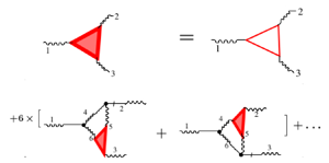
In this subsection, we will bring all the things we have considered together and introduce triangular re-summation of the triple correlator, the latter being the main focus of this work. It has three appearances, shown in figure 1: empty thin red triangle for first-order contribution ${}^{3}\!F^{{{ I}}}$, empty thick red triangle for third-order contribution ${}^{3}\!F^{{{III}}}$, and filled thick red triangle for the full correlator ${}^{3}\!F$.

One of the main points of this paper may be recognized by comparing diagrams for ${}^{3}\!F^{{{I}}}$ in figure 6 and for ${}^{3}\!F^{{{III}}}$ in figure 7. Note that our definition of the correlator involves the permutation operator ${\boldsymbol P}_{123}$, defined by (2.12a) and (2.13). First notice that (d–i) of figure 7 contain a vertex marked by a red circle, and the Green's functions connected to this vertex form precisely the diagrams of the ${}^{3}\!F^{{{I}}}$ shown in figure 6. As we will see below (see (4.6)), this fact allows us to write a compact expression for ${}^{3}\!F^{{{III}}}$,

(4.1)\begin{equation} \left.\begin{gathered} {}^{3}\! F_{123}^{{{III}}}= {\boldsymbol P}\int \frac{{\rm d} \boldsymbol{k}_4}{{(2{\rm \pi})^d}}\, {}^4T_{2346} V_{146} \times [ V_{425}F_2+V_{245} F_4 ] \, {}^{3}\!F_{356}^{{{ I}}}, \\ \boldsymbol{k}_5=\boldsymbol{k}_4+ \boldsymbol{k}_2\ {\rm and}\ \boldsymbol{k}_6=\boldsymbol{k}_4- \boldsymbol{k}_1, \end{gathered}\right\} \end{equation}

expressed in terms of the first-order correlator as follows from figures 7(g,h). This fact has deep consequences, as we will see below.

The permutation operator ${\boldsymbol P}_{123}$ acting on the two diagrams of figure 7 produces six diagrams. These diagrams can be grouped into a triad of diagrams that involves three vertices, with rotational $C_3$ symmetry, and three tails of Green's functions ordered chronologically inside the triangle from the present time $t=0$ in the simultaneous correlator back to all past times $t_j< 0$, as required by the casualty principle. We will refer to this object as a ‘third-order triad’ and depict it by the thick red triangle.

Notice that the bare Green's function and bare double correlation in the Dyson–Wyld line re-summation are called reducible fragments, which can be separated from the body of a diagram by cutting two lines. Bearing this in mind, we can clarify them as ‘double-line’ reducible diagrams. Such a name immediately suggests the existence of ‘triple-line reducible diagrams’. Indeed, our triad diagrams can be separated from the body of a diagram by cutting three Green's functions entering this time zone. We call these objects ‘triple-line reducible triads’ (of $C_3$ symmetrical groups of diagrams). Up to now, we met in figure 6 first-order triple-line reducible triads (with one vertex) and in figure 7 third-order triple-line reducible triads with three vertices, shown e.g. in figure 7(d) by a blue square.

Let us examine again figure 7(d). The red (oldest) time zone has three incoming Green's functions entering it with straight lines. The red time zone is in turn inside the earlier, blue time zone, which has three straight lines entering it. This is an example of the triangular telescopically nested time-ordered reducible triads. Higher-order diagrams for the simultaneous triple correlators will have multiple zones nested in similar manner. These zones will sum up the fully dressed triple correlator.

Indeed, analysis of the higher-order diagram for ${}^{3}\!F$ shows that besides two first-order triads in the first row of figure 7 (thin red triangles) one finds diagrams in which instead of the first-order triads, one meets third-order triads (thick red triangles). These diagrams represent fifth-order triads, which in turn can be found in even higher-order diagrams, etc. This possibility originates first from the fact that the perturbation diagrammatic series involves all topologically possible diagrams, and second because all diagrammatic rules, including $1/N$ symmetry rules and time integration rules, are applicable not only to the whole diagrams but also to any of their fragments. Therefore, there is a mechanism for the infinite resuming of telescopically nested, chronologically ordered triple-line reducible triads, appearing instead of the earliest time zones, resulting in the fully dressed triple correlator ${}^{3}\!F_{123}$.

The Dyson line re-summation leads to a fully dressed Green's function. The Wyld re-summation leads to the fully dressed double correlator. The triangular re-summation of the triple-line reducible triads suggested here leads to a fully dressed simultaneous triple correlator, as we will show in § 4.3.

4.2. Triangular re-summation of diagrams for quadruple correlators ${}^{4}\!F_{1234}$

4.2.1. Identifying ${}^{3}\!F ^{{{I}}}$ triad in diagrams for ${}^{4}\!F^{{{II}}}$

Analysing the second-order diagrams ${}^{2}\!\!\mathcal {A}_{1,234}$ and ${}^{2}\!{\mathcal {B}}_{12,34}$ for ${}^{4}\!\mathcal {F}_{1234}$, shown in figures 3(b,c), as before, we replace the (three) double correlators by a sum of two auxiliary Green's functions according to (3.2). In such a case, each of the diagrams produces $2^3$ diagrams. Out of those $2\times 2^3=16$ diagrams, only three of them, shown in figures 10(a,b), survive for the same-time case after frequency integration required by (3.1b). Note that the diagram in figure 10(b) appears twice in different orientations. This removes the factor ${1}/{2}$ in front of it. The disappearance of the $1/2$ factor occurs as a manifestation of the $1/N$ symmetry rule because the diagram in figure 10(b) lost reflecting symmetry with respect to the vertical line, present (together with prefactor $1/2$) in the diagram depicted in figure 3(c).

Analytically, diagrams in figure 10 can be written as ${^4\! F}_{1234} ^{{{II}}}=\underset {1234}{\boldsymbol P} [{}^2\! A _{1,234} + {}^{2}\!B_{12,34} ]$, where

(4.2a)\begin{equation} {}^{2}\! A _{1,234} = \tfrac12 V_{14\bar 5} V_{523 } { F}_2 { F}_3 { F}_4 T,\ {}^2\! B_{12,34} = F _3 F _4 F _ {1+4} V_{13\bar 5 } V_{235}T , \ \ T \equiv T_{1234} T_{235}, \end{equation}

with $\boldsymbol{q}_5= \boldsymbol{q}_1+\boldsymbol{q}_4 =-(\boldsymbol{q}_2+\boldsymbol{q}_3)$. The time integral $T$ here was found with the help of diagrammatic rules formulated in § 3.3. It reduces to a product of the triad and quartic interaction times. Together with diagrams in figures 6(e–g), this allows us to recognize that the sum of the diagrams presented in figures 10(b,c) include the correlator ${}^{3}\!F_{235}^{{{I}}}$, shown in figure 10(d) as red filled circle. Analytically, this reads

(4.2b)\begin{equation} {^4\! F}_{1234} ^{{{II}}}= 3 T_{1234}(V_{145} F_4 ) F^{{{I}}}_{235} . \end{equation}

We see that the first contribution of ${}^4\! F_{1234} ^{{{II}}}$ to the four-point correlator contains the first contribution ${}^{3}\!F^{{{ I}}}_{235}$ to the three-point correlator. We will show below that this statement generalizes to higher orders as follows. The $(n+1)$th order of ${}^4\! F_{1234} ^{n+1}$ involve an $n$th-order contribution of ${}^{3}\!F^n$. Consequently, the fully dressed fourth-order correlator depends on the fully dressed third-order correlator. This is the essence of the triangular re-summation, and it underlines the key role played by the third-order correlator.

4.2.2. Identifying ${}^{3}\!F^{{{I}}}$ and ${}^{3}\!F^{{{III}}}$ triads in the weakly connected spine diagrams for ${}^{4}\!F^{{{IV}}}$

Recall that diagrams in figures 10(b,c) are weakly connected in the sense that they can be divided into two parts by cutting only one line, sometimes referred to as a ‘spine’. Using diagrammatic rules for ${}^{4}\!F^{(4)}_{1234}$ formulated in § 2.4, we found all the weakly connected spine diagrams shown in figures 8, 9 and 11. We divide the diagrams into these three figures by the position of the earliest (red) time zone relative to the spine $G_5$. Figure 8 shows 18 diagrams with the earliest time zone to the right of the Green's function $G_5$ in the (678)-triangle; figure 9 includes 8 diagrams with the (145)-time zone to the left of $G_5$; and figure 11 involves six diagrams with two earliest times on either side of $G_5$.

The diagrams of figures 8, 9 and 11 are grouped in such a way that the triple correlator ${}^{3}\!F^{{{I}}}$ is identifiable in each row. That is, each line contains equivalent diagrams except for the position of the true Green's function entering the earliest time zone. Consequently, each row sums to the diagram in the right-hand column containing the third-order correlator in the third-order ${}^{3}\!F^{{{III}}}$ shown as a thin red triangle.

Consider the diagrams in figure 8. The six resulting diagrams on the right-hand side have the same structure connecting two parts by leg $5$. One part is the block of $G_1G_4 V_{145}$ with three legs. The second part consist of the structures in which we recognize one of the diagrams for ${}^{3}\!F^{{{III}}}$, shown figure 7.

Therefore, similarly to (4.2b), the sum of all diagrams in figure 8 for ${}^{4}\!F^{{{IV}}}$ (denoted as ${}^{4,\alpha }F^{{{IV}}} _{1234}$) can be presented via ${}^3{F^{{{III}}}}$:

(4.3a)\begin{equation} ^{4,\alpha}\! F_{1234}^{{{IV}}} = 3 \, T_{1234}(V_{145} F_4 ) \, {}^{3\! } F^{{{III}}}_{235} . \end{equation}

Comparing (4.2b) and (4.3a), we see that: (i) the fourth-order correlator ${}^4\! F_{1234} ^{n+1}$ of any order always includes quadruple interaction time $T_{1234}$, originated from integration in the latest time zone with four external legs of the Green's function $G_1G_2G_3G_4$; (ii) the earliest time zone, (235) in this case, denotes the place where the triple correlator appears after the triangular re-summation.

Considering diagrams with the earliest (145) time zone in figure 9, we see that figures 9(a–d) have the same structure, summed to the triple correlator ${}^{3}\!F^{{{I}}}_{145}$ times three-point objects, denoted as $X^{{{A}}}$, $X^{{{B}}}$, $X^{{{C}}}$ and $X^{{{D}}}$. The sum of these diagrams is given by

(4.3b) \begin{gather} \left.\begin{gathered} ^{4,\beta}\! F_{1234}^{{{IV}}} = 3 T_{1234} \, {}^{3}\! F^{{{I}}}_{145} [ X^{{{A}}}_{5,23}+X^{{{B}}}_{5,23}+X^{{{C}}}_{5,23}+X^{{{D}}}_{5,23}], \quad \boldsymbol{k}_5=\boldsymbol{k}_1+\boldsymbol{k}_4,\\ X^{{{A}}}_{5,23} = V_{567} V_{6\bar 2 8 } V_{8\bar 3 7}F_3 F_4 , \quad X^{{{B}}} _{5,23} = V_{756} V_{268 } V_{8\bar 3 7}F_3 F_6 ,\quad \ldots . \end{gathered}\right\} \end{gather}

Equations for $X^{{{ C}}}_{5,23}$ and $X^{{{ D}}}_{5,23}$ in (4.3b) can be reconstructed easily from their diagrammatic representation in figure 9.

The last group of the weakly connected spine diagrams with two earliest time zones is shown in figure 11. These diagrams sum up into one diagram, with the product of two triple correlators shown in in figure 11(c-iii). The corresponding analytical expression is

(4.3c)\begin{equation} ^{4,\gamma}\! F_{1234}^{{{IV}}} = 9 T_{1234} \,{}^{3}\!F^{{{I}}} _{145}\int \frac{{\rm d} \boldsymbol{k}_6}{(2{\rm \pi})^d}\,T_{13468}\,{}^{3}\!F^{{{I}}} _{378} V_{268}V_{657} . \end{equation}

Remarkably, this contribution is proportional to the square of the triple correlator ${}^{3}\!F^{{{I}}}$.

4.2.3. Identifying ${}^{3}\!F^{{{I}}}$ in the compact square diagrams for ${}^{4}\!F^{{{IV}}}$

As seen in figure 5, there are eight compact ‘square’ diagrams for the quadruple correlator ${}^{4}\!F^{{{IV}}}$. Consequently, they produce $8\times 2^4=128$ child diagrams, but only 22 of them, shown in figures 17 and 18, contribute to the simultaneous correlator. Similar to the previous subsubsection, here we show how all of them can be grouped in triads, each of which represents the triple correlator ${}^{3}\!F^{{{I}}}$. We identify the triads of diagrams such that all elements in the diagrams in each triad are identical, except one vertex, where the ‘true’ Green's function occupies each of the three positions in turns, and the other two positions are occupied by auxiliary Green's functions.

First, we separate all diagrams into two groups: those with one earliest time zone shown in figures 12 and 13, and those with two earliest time zones shown in figure 14.

The biggest group with one such zone will be further divided into several topologically different subgroups as follows. Since the diagrams are under the permutation operator, we redraw the diagrams (by rotations or by mirroring) in such a way that the earliest time zone will be placed in the upper right corner of the diagram marked by red circle. We then label all lines as shown e.g. in figure 12(a-i).

Now we will classify the diagrams by the number of the external real Green's functions on the vertex 1, 3 and 4. We call the diagrams ‘identical by Green's functions’ if their external Green's functions are identical. This set of lines does not include lines labelled by 2, 5, which connect to the earliest time zone. We recall that all vertices must be connected to one of the external true Green's functions by the true Green's functions with the same orientations.

In a subgroup with at least one true Green's-function there are two options: in which either $G_1$ or $G_2$ are true Green's function. The subgroup in which $G_3$ is a true Green's function is not distinct: it topologically coincides with the $G_1$ subgroup by mirroring in the 2–4 line that connects $G_2$ and $G_4$.

Consider the subgroup of diagrams with external true Green's function $G_1$. These diagrams are shown in figure 12 (a-i a-iii). From general requirements, its topology must include $G_7$ and $G_8$ true Green's functions that connect 3- and 4-vertices to a 1-vertex with true Green's function $G_1$. This subgroup has only three diagrams, shown in figures 12(a-i), 12(a-ii) and 12(a-iii). These three diagrams form the first triad, which sums to the diagram in figure 12(a-iv) that involves the triple correlator ${}^{3}\!F^{(1)}_{256}$.

Next, the $G_4$ subgroup must include $G_7$ and $G_8$ true Green's functions that connect the 4 vertex with 3- and 1-vertices. This subgroup has only two diagrams, shown in figures 12(b-i) and 12(b-ii), forming the triad that sums to the diagram in figure 12(b-iii) that involves the triple correlator.

There are nine diagrams with two true Green's functions labelled either 1 and/or 3 and 4. The first six diagrams involve $G_1$ and $G_4$. Three of them, collected in figures 12(c-i), 12(c-ii) and 12(c-iii), have auxiliary Green's function $G_8$, oriented down by a straight line. They are summarized in the diagram in figure 12(c-iv) that involves the same triple correlator ${}^{3}\!F^{(1)}_{256}$. The remaining three diagrams with auxiliary Green's functions $G_8$, oriented up, are summarized in the diagram in figure 12(d-iv). The last triad with two real Green's functions $G_1$ and $G_3$ create the diagram in figure 12(e-iv), with the same triple correlator ${}^{3}\!F^{(1)}_{256}$.

The subgroup with three true Green's-functions $G_1$, $G_2$ and $G_3$ is shown in figure 13. They create two subgroups, with auxiliary Green's function G ₈ oriented either up or down. The first triad creates a diagram in figure 13(a-iv). Considering the diagram in figure 13(b-i) as two diagrams (with prefactor $1/2$) and rotating one of them around the 2–4 line, we have a second triad that creates the diagram in figure 13(b-iii).

Analytical expressions for ${}^{4\delta }\!F^{{{IV}}}_{1234}$, originated from diagrams $X_1,X_2,\ldots, X_7$ depicted in figures 12 and 13, are as follows:

(4.4)\begin{equation} \left.\begin{gathered} ^{4\delta}\!F^{{{IV}}} _{1234}= T_{1234} \underset{1234}{\boldsymbol P}\left \{ \int \frac{{\rm d} \boldsymbol{k}_5}{{(2{\rm \pi})^d}}\, {}^{3}\!F^{(1)}_{256} J _{1234}^{\square}\right\},\\ {\boldsymbol k_6} ={\boldsymbol k_2} + {\boldsymbol k_5}, \quad J_{1234}^\square = \sum_{i=1}^7 X_i, \\ X_1 = 6 T_{2357}T_{23458}V_{1 \bar{5} 8}V_{\bar 7 3 6}V_{\bar 8 4 7}F_3 F_4,\\ X_2= 3 (T_{2357}+T_{1268})T_{12378}V_{8 1 \bar 5}V_{\bar 7 6 3 }V_{4 7 \bar 8}F_1 F_3, \\ X_3= 6 T_{2357}T_{23458} V_{1 \bar{5} 8}V_{\bar{7} 3 6}V_{4 7 \bar{8}}F_3 F_8, \quad X_4= 6 T_{2357}T_{23458}V_{1 \bar 5 8}V_{\bar 7 3 6}V_{4 7\bar 8}F_3 F_8, \\ X_5= 6 T_{2357}T_{23458}V_{1 \bar 5 8}V_{\bar 7 3 6}V_{\bar 8 4 7}F_4 F_7, \quad X_6= 6 T_{2357}T_{23458}V_{1 \bar 5 8}V_{3 6 \bar 7}V_{4 7\bar 8}F_7 F_8, \\ X_7= 6 T_{2357}T_{23458}V_{1 \bar 5 8}V_{3 6 \bar 7}V_{4 7\bar 8}F_7 F_8. \end{gathered}\right\} \end{equation}

The ‘square’ superscript denotes the sum of the square diagrams in figures 12 and 13. The second group of diagrams with two earlier time zones consists only of four diagrams. We used the diagram ${}^{4}\!C^{{{VII}}}$ in figures 14(a-iii) and 14(b-i), putting prefactor $1/2$ in front of them. After that, figures 14(a-i), 14(a-ii) and 14(a-iii) are summed to figure 14(a-iv), and figures 14(b-i) and 14(b-ii) are summed to figure 14(b-iii). In turn, figures 14(a-iv) and 14(b-iii) (repeated as figures 14(c-i) and 14(c-ii)) can be summed to figure 14(c-iii), which involves two triple correlators, ${}^{3}\!F^{{{I}}}_{256}$ and ${}^{3}\!F^{{{I}}}_{478}$. An analytical expression for the sum of all diagrams with two earliest time zones is

(4.5)\begin{equation} ^{4\varepsilon}\!F^{{{IV}}} _{1234} = T_{1234} \underset{1234}{\boldsymbol P}\left \{ \int \frac{{\rm d} \boldsymbol{k}_5}{{(2{\rm \pi})^d}}\, {}^{3}\!F^{{{ I}}} _{256} \, {}^{3}\!F^{{{I}}} _{478} \times (T_{23458}+T_{12467} ) V_{15\bar 8}V_{3\bar 6 7}\right \}. \end{equation}

Similar to (4.3c), here the contribution to the fourth-order four-point correlator comes from the product of two three-point correlators of the first order, ${}^{3}\!F_{123}^{{{I}}}$. Analysing the structure of the diagrammatic technique, we expect that in the higher-order diagrams, terms with a product of three or more correlators ${}^{3}\!F_{123}^{{{I}}}$ will appear.

4.3. Full triangular re-summations for ${}^{3}\!F_{123}$ and ${}^{4}\!F_{1234}$

In the previous subsections, we demonstrated how the sum of six initial diagrams for ${}^{3}\!F_{123}^{{{III}}}$ presented in figure 7 fuses into two diagrams in figures 7(b,c) involving ${}^{3}\!F^{{{I}}}$. Similarly, the sum of two diagrams for ${}^{4}\!F_{1234}^{{{II}}}$ in figure 10 combines to one diagram figure 10(d) with ${}^{3}\!F ^{{{I}}}$. Moreover, the sum of 18 diagrams for ${}^{4}\!F_{1234}^{{{IV}}}$ in figure 8 combines to six diagrams involving ${}^{3}\!F^{{{I}}}$, which in turn fuse into just one diagram with ${}^{3}\!F ^{{{III}}}$, presented analytically by (4.3a). In exactly the same way, the rest of the diagrams for ${}^{4}\!F_{1234}^{{{IV}}}$ shown in figures 9–14 were summarized in these figures to diagrams involving the triple correlator ${}^{3}\!F^{{{I}}}$. These findings are not a miracle, but a deep consequence of fundamental features of the perturbation approach reflected in the diagrammatic technique and the crucial role that is played by the three-point correlator.

Namely, the diagrammatic series involves all topologically possible diagrams, satisfying general restrictions, described in § 2.4. These restrictions together with the $1/N$ rule, prescribing the numerical prefactor, have local character, i.e. they are applicable to the entire diagram, or to any of its fragments. For example, any diagram for ${}^{3}\!F_{123}$ has three external Green's functions $G_1$, $G_2$ and $G_3$ entering the diagram by straight lines. Similarly, any earliest time zone also has three ‘boundary’ Green's functions, say $G_k$, $G_l$ and $G_m$, entering the zone in the same way. Therefore, the sum of all diagrams inside the earliest time zone of $(2n+1)$th order (with $(2n+1)$ vertices) gives exactly the triple correlator of $(2n+1)$th order, ${}^{3}\!F^{n+1}_{klm}$. This is exactly what happened in all diagrams with the first-order earliest time zones (coloured in red), summarized to ${}^{3}\!F^{{{I}}}$, while the diagrams in figure 8 with the third-order earliest time zones (coloured in blue) were summarized to ${}^{3}\!F^{{{III}}}$.

Consider first full triangular re-summation for the triple correlator ${}^{3}\!F_{123}$. Figure 15(a) just resembles the diagram in figure 6(b) for ${}^{3}\!F^{{{I}}}_{123}$, while figure 15(b-i–b-iii) shows re-summation diagrams for ${}^{3}\!F^{{{III}}}_{123}$, with the result ${}^{3}\!F^{{{III}}}_{123}\propto ^{3}\! F^{{{I}}}_{123}$, as indicated by (4.1). The next step is shown in figure 15(b). Comparing figures 15(b) and 15(c), we see the pattern that illustrates the essence of the triangular re-summation. Namely, ${}^{3}\! F^{{{III}}}_{123}$ depends on ${^1}\! F^{{{I}}}_{123}$ in the same way as ${}^{3}\!F^{{{V}}}_{123}$ depends on ${}^{3}\!F^{{{III}}}_{123}$. We can continue this iteration ad infinitum; see the result in figure 15(c). Clearly, this procedure does not create high-order diagrams for ${}^{3}\!F^{{{III}}}_{123}$ of a more complicated topological structure. These diagrams are replaced by ‘…’ (an ellipsis) in figure 15(c), which presents the entire series for ${}^{3}\!F = {}^{3}\!F^{{{I}}}_{123}+ {}^{3}\!F^{{{III}}}_{123}+{}^{3!}F^{{{V}}}_{123}+\cdots$. Analytically, we have

(4.6)\begin{equation} {}^{3}\!F_{123} = {}^{3}\! F_{123}^{I} + 6 \underset{123 }{\boldsymbol P}\int \frac{{\rm d} \boldsymbol{k}_4}{(2{\rm \pi})^d}\,T_{2346} V_{146} \times [ V_{425}F_2+V_{245} F_4 ] \, {}^{3}\!F_{356} + \cdots. \end{equation}

This equation represents the essence of triangular re-summation for the fully dressed triple correlator ${}^{3}\!F_{123}$, as it represents ${}^{3}\!F_{123}$ through the infinite series that itself involves ${}^{3}\!F_{123}$. If one neglects higher-order contributions replaced in (4.6) by an ellipsis, then this equation becomes a closed equation for ${}^{3}\!F_{123}$. Clearly, this procedure is an uncontrolled approximation. Currently, this equation looks linear since the higher-order terms are represented as an ellipsis. Analysing higher-order contributions, we found diagrams with two, three and more earliest time zones, giving birth to contributions to (4.6) proportional to $(^{3}\!F) ^2$, $(^{3}\!F)^3$, and so on.

Figure 15. First triple-irreducible diagrams in the triangular re-summation for ${}^{3}\!F^{(\infty )}$: (a) the ${}^{3}\!F_{123}^{{{I}}}$ correlator; (b) the ${}^{3}\!F_{123}^{{{III}}}$ correlator; and (c) the ${}^{3}\!F_{123}^{{{V}}}$ correlator. (d) Diagrams yielding integral equation (4.6) as a result of full triangular re-summation for ${}^{3}\!F_{123}$. Triangular re-summation of the full triple correlator given by (4.6): the full triple correlator (filled triangle) is expressed as a sum of a bare triple correlator (thin triangle) and an infinite diagrammatic series that depends on the triple correlator itself.

Based on (4.6), consider an inverse energy cascade in the fractional dimension $d=\frac 43+ x$ close to the critical dimension $d_0=\frac 43$. Here, there are two limiting cases: (i) constant energy flux $\varepsilon$, or (ii) constant energy ${}^{2}\!F$. When $\varepsilon =\textrm {const}$ in the limit $x\to 0$, the energy is ${}^{2}\!F\to \infty$. We focus on the latter case, when the energy ${}^{2}\!F(\boldsymbol{k})$ is kept finite. Then in the limit $x\to 0$, the energy flux $\varepsilon$ (together with ${}^{3}\! F$) vanishes. In this case, (4.6) becomes a nonlinear homogeneous equation with powers of full triple correlators on its right-hand side. This equation has a trivial solution ${}^{3}\! F_{123}=0$. This is a demonstration that the triple simultaneous correlator is zero under these assumptions ($d=\frac 43$ and finiteness of the energy), not only in the leading order (as shown in L'vov et al. Reference L'vov, Pomyalov and Procaccia2002) but in all orders, i.e. fully dressed correlator ${}^{3}\! F=0$.

The diagrams for the four-point simultaneous correlator ${}^{4!}F_{1234}$ can also be triangular re-summed. This is shown in figure 16. We denote ${}^{4}\!F_{1234}$ as a red thick-filled square. The simplest diagram, in figure 16(a-ii), originates from the infinite re-summation of the diagram for ${}^{4}\!F_{1234}^{{{II}}}$ in figure 10(d), where ${}^{3}\!F^{{{I}}}$ is summed up to the full correlator. Graphically, this part of the triangular re-summation is depicted by replacing the thin triangle by thick filled triangle. The triangular re-summation includes all diagrams in figure 8. Four rows of diagrams in figure 9 (after inversion over a spine Green's function $G_5$) serve as the first terms of the triangular re-summation that leads to diagrams in figures 16(a-iii)–16(a-vi). In the same way, diagrams in figure 11 produce figure 16(a-vii), proportional to $(^{3}\!F)^2$, and compact square diagrams in figures 12 and 13 give, after re-summation, diagrams in figures 16(b-i) and 16(b-ii). Remarkably, compact square diagrams in figure 14 with two earliest time zones create the diagram in figure 16(b-iii). This diagram is proportional to the square of the full triple correlator ${}^{3}\!F$. Higher-order terms, represented by dots, can also be triangular re-summed.

Figure 16. Full triangular re-summation for the four-point correlator ${}^{4}\!F_{1234}$.

Analytical expressions for various contributions to ${}^{4}\!F_{1234}$, denoted ${}^{4}\!F_{1234}^{{{A1}}},\ldots, {}^{4}\!F_{1234}^{{{A6}}}$, ${}^{4}\!F_{1234}^{{{B1}}}$, ${}^{4}\!F_{1234}^{{{B2}}}$ and ${}^{4}\!F_{1234}^{{{B3}}}$, can be reconstructed straightforwardly from the corresponding diagrams, e.g.

(4.7) \begin{align} \left.\begin{aligned} ^{4}\!F_{1234}^{{{A1}}}&= 3\, {}^{3}\!F_{235} F_4 V_{145},\\ {}^{4}\!F_{1234}^{{{A2}}}&= 3\, {}^{3}\!F_{235} F_4 \int \frac{{\rm d} \boldsymbol{k}_6}{(2{\rm \pi})^2}\,V _{168}V_{657}V_{847}F_7,\quad\ldots\\ ^{4}\!F_{1234}^{{{A6}}}&= 9 \, {}^{3}\!F_{235} \int \frac{{\rm d} \boldsymbol{k}_6}{(2{\rm \pi})^2}\,V _{168}V_{657} \, {}^{3}\!F_{235},\\ {}^{4}\!F_{1234}^{{{B1}}}&= 6 F_3 F_4 \int \frac{{\rm d} \boldsymbol{k}_5}{(2{\rm \pi})^2}\,V _{156}V_{847}V_{673} \, {}^{3}\!F_{256},\quad\ldots\\ {}^{4}\!F_{1234}^{{{B3}}}&= \frac32 \int \frac{{\rm d} \boldsymbol{k}_5}{(2{\rm \pi})^2}\,V _{158}V_{367} \,{}^{3}\!F_{256}\,{}^{3}\!F_{478}.\end{aligned}\right\} \end{align}

These equations present fully dressed quadruple correlator ${}^{4}\!F_{1234}$ as a series in powers of fully dressed triple correlator ${}^{3}\!F$, explicitly involving linear and quadratic contributions. Some diagrams with five or more vertices will give contributions of third, fourth and higher powers of ${}^{3}\!F$.

In particular, this means that in the inverse energy cascade in a dimension near the critical $d =\frac 43+x$, the dressed fourth-order correlator ${}^ {4}\!F_{1234}$ vanishes in the limit $x \to 0$ with finite energy. Moreover, there is every reason to believe that this statement is valid for all high-order correlators ${}^{n}\!F$ with $n=4, 5,\ldots$. If so, then the statistics of turbulence in $d =\frac 43$ becomes Gaussian when all cumulants vanish, and is very close to the Gaussian statistics for $d =\frac 43+x$. We think that this explains the experimental observation that the statistics of the inverse energy cascade is close to Gaussian even for $d=2$.

References

Boffeta, G., Celani, A. & Vergassola, M. 2000 Inverse energy cascade in two-dimensional turbulence: deviations from Gaussian behavior. Phys. Rev. E 61, R29.CrossRefGoogle Scholar
Boffetta, G. & Ecke, R.E. 2012 Two-dimensional turbulence. Annu. Rev. Fluid Mech. 44 (1), 427451.CrossRefGoogle Scholar
Frisch, U. 1995 Turbulence: The Legacy of A.N. Kolmogorov. Cambridge University Press.CrossRefGoogle Scholar
Kolmogorov, A.N. 1941 Equations of turbulent motion in an incompressible fluid. Dokl. Akad. Nauk SSSR 30, 299303.Google Scholar
Kraichnan, R. & Montgometry, D. 1980 Two-dimensional turbulence. Rep. Prog. Phys. 43, 547.CrossRefGoogle Scholar
Landau, L.D. & Lifshitz, E.M. 1980 Statistical Physics, vol. 5. Butterworth Heinemann.Google Scholar
Landau, L.D. & Lifshitz, E.M. 2013 Fluid Mechanics: Landau and Lifshitz: Course of Theoretical Physics, vol. 6. Elsevier.Google Scholar
L'vov, V.S., Lvov, Y.V. & Pomyalov, A. 2000 Anisotropic spectra of acoustic turbulence. Phys. Rev. E 61 (3), 2586.CrossRefGoogle Scholar
L'vov, V.S., Pomyalov, A. & Procaccia, I. 2002 Quasi-Gaussian statistics of hydrodynamic turbulence in $4/3+ \varepsilon$ dimensions. Phys. Rev. Lett. 89 (6), 64501.CrossRefGoogle Scholar
L'vov, V.S. & Procaccia, I. 1995 Exact resummations in the theory of hydrodynamic turbulence: 0. Line-resummed diagrammatic perturbation approach. arXiv:chao-dyn/9502010.Google Scholar
Martin, P.C., Siggia, E.D. & Rose, H.A. 1973 Statistical dynamics of classical systems. Phys. Rev. A 8, 423437.CrossRefGoogle Scholar
Pope, S.B. 2000 Turbulent Flows. Cambridge University Press.CrossRefGoogle Scholar
Tabeling, P. 2002 Two-dimensional turbulence: a physicist approach. Phys. Rep. 362, 162.CrossRefGoogle Scholar
Wyld, H.D. 1961 Formulation of the theory of turbulence in an incompressible fluid. Ann. Phys. (N.Y.) 14, 143165.CrossRefGoogle Scholar
Zakharov, V.E. & L'vov, V.S. 1975 Statistical description of nonlinear wave fields. Radiophys. Quantum Electron. 18 (10), 10841097.CrossRefGoogle Scholar
Zakharov, V.E., L'vov, V.S. & Musher, S.L. 1972 Transient behavior of a system of parametrically excited spin waves. Sov. Phys. Solid State 14 (3), 16.Google Scholar
Zakharov, V.E., L'vov, V.S. & Starobinets, S.S. 1975 Spin-wave turbulence beyond the parametric excitation threshold. Sov. Phys. Usp. 17 (6), 896.CrossRefGoogle Scholar