


1. Introduction
1.1. Dynamical systems and entropy
Topological pressure and its variational principle have been significant in several fields, including the dimension theory of dynamical systems. Recently, Feng and Huang devised an innovative invariant called weighted topological pressure for factor maps between dynamical systems and proved its variational principle [Reference Feng and HuangFH16]. Their work inspired Tsukamoto to suggest a new definition of this invariant [Reference TsukamotoTsu22]. He also established a variational principle, revealing the non-trivial coincidence of the two definitions. Tsukamoto focused on the simplest case with two dynamical systems.
In this paper, we extend Tsukamoto’s definition to the case of an arbitrary number of dynamical systems and prove its variational principle. With our result, we can plainly calculate the Hausdorff dimension of self-affine sponges, a topic studied by Kenyon and Peres [Reference Kenyon and PeresKP96]. Furthermore, we will show in §6 that we can determine the Hausdorff dimension of certain sofic sets embedded in higher-dimensional Euclidean space.
We review the basic notions of dynamical systems in this subsection. Refer to the book of Walters [Reference WaltersWal82] for the details.
A pair
 $(X, T)$
is called a dynamical system if X is a compact metrizable space and
$(X, T)$
is called a dynamical system if X is a compact metrizable space and
 $T: X \rightarrow X$
is a continuous map. A map
$T: X \rightarrow X$
is a continuous map. A map
 $\pi : X \rightarrow Y$
between dynamical systems
$\pi : X \rightarrow Y$
between dynamical systems
 $(X, T)$
and
$(X, T)$
and
 $(Y, S)$
is said to be a factor map if
$(Y, S)$
is said to be a factor map if
 $\pi $
is a continuous surjection and
$\pi $
is a continuous surjection and
 $\pi \circ T = S \circ \pi $
. We sometimes write as
$\pi \circ T = S \circ \pi $
. We sometimes write as
 $\pi : (X, T) \rightarrow (Y, S)$
to clarify the dynamical systems in question.
$\pi : (X, T) \rightarrow (Y, S)$
to clarify the dynamical systems in question.
For a dynamical system
 $(X, T)$
, denote its topological entropy by
$(X, T)$
, denote its topological entropy by
 $h_{\mathrm {top}}(T)$
. Let
$h_{\mathrm {top}}(T)$
. Let
 $P(f)$
be the topological pressure for a continuous function
$P(f)$
be the topological pressure for a continuous function
 $f: X \rightarrow \mathbb {R}$
(see §2 for the definition of these quantities). Let
$f: X \rightarrow \mathbb {R}$
(see §2 for the definition of these quantities). Let
 $\mathscr {M}^T(X)$
be the set of T-invariant probability measures on X and
$\mathscr {M}^T(X)$
be the set of T-invariant probability measures on X and
 $h_\mu (T)$
the measure-theoretic entropy for
$h_\mu (T)$
the measure-theoretic entropy for
 $\mu \in \mathscr {M}^T(X)$
(see §3.2). The variational principle then states that [Reference DinaburgDin70, Reference GoodmanGm71, Reference GoodwynGw69, Reference RuelleRu73, Reference WaltersWal75]
$\mu \in \mathscr {M}^T(X)$
(see §3.2). The variational principle then states that [Reference DinaburgDin70, Reference GoodmanGm71, Reference GoodwynGw69, Reference RuelleRu73, Reference WaltersWal75]
 $$ \begin{align*} P(f) = \sup_{\mu \in \mathscr{M}^T(X)} \bigg( h_\mu(T) + \int_X f\,d\mu \bigg). \end{align*} $$
1.2. Background
We first look at self-affine sponges to understand the background of weighted topological entropy introduced by Feng and Huang. Let
 $m_1, m_2, \ldots , m_r$
be natural numbers with
$m_1, m_2, \ldots , m_r$
be natural numbers with
 $m_1 \leq m_2 \leq \cdots \leq m_r$
. Consider an endomorphism T on
$m_1 \leq m_2 \leq \cdots \leq m_r$
. Consider an endomorphism T on
 $\mathbb {T}^r = \mathbb {R}^r/\mathbb {Z}^r$
represented by the diagonal matrix
$\mathbb {T}^r = \mathbb {R}^r/\mathbb {Z}^r$
represented by the diagonal matrix
 $A = \mathrm {diag}(m_1, m_2, \ldots , m_r)$
. For
$A = \mathrm {diag}(m_1, m_2, \ldots , m_r)$
. For
 $D \subset \prod _{i=1}^r \{0, 1, \ldots , m_i-1\}$
, define
$D \subset \prod _{i=1}^r \{0, 1, \ldots , m_i-1\}$
, define
 $$ \begin{align*} K(T, D) = \bigg\{\! \sum_{n=0}^{\infty} A^{-n}e_n \in \mathbb{T}^r \bigg| e_n \in D \bigg\}. \end{align*} $$
This set is compact and T-invariant, that is,
 $TK(T, D) = K(T, D)$
.
$TK(T, D) = K(T, D)$
.
These sets for
 $r = 2$
are known as Bedford–McMullen carpets or self-affine carpets. Figure 1 exhibits a famous example, the case of
$r = 2$
are known as Bedford–McMullen carpets or self-affine carpets. Figure 1 exhibits a famous example, the case of
 $D = \{(0,0), (1,1), (0,2)\} \subset \{0, 1\} \times \{0, 1, 2\}$
. The analysis of these sets is complicated compared with ‘self-similar’ sets. Bedford [Reference BedfordBed84] and McMullen [Reference McMullenMcM84] independently studied these sets and showed that, in general, their Hausdorff dimension is strictly smaller than their Minkowski dimension (also known as box-counting dimension). Figure 1 has Hausdorff dimension
$D = \{(0,0), (1,1), (0,2)\} \subset \{0, 1\} \times \{0, 1, 2\}$
. The analysis of these sets is complicated compared with ‘self-similar’ sets. Bedford [Reference BedfordBed84] and McMullen [Reference McMullenMcM84] independently studied these sets and showed that, in general, their Hausdorff dimension is strictly smaller than their Minkowski dimension (also known as box-counting dimension). Figure 1 has Hausdorff dimension
 $\log _2{(1+2^{\log _3{2}})} = 1.349 \cdots $
and Minkowski dimension
$\log _2{(1+2^{\log _3{2}})} = 1.349 \cdots $
and Minkowski dimension
 $1 + \log _3{\tfrac {3}{2}} = 1.369 \cdots $
.
$1 + \log _3{\tfrac {3}{2}} = 1.369 \cdots $
.

Figure 1 First four generations of a Bedford–McMullen carpet.
The sets
 $K(T, D)$
for
$K(T, D)$
for
 $r \geq 3$
are called self-affine sponges. Kenyon and Peres [Reference Kenyon and PeresKP96] calculated their Hausdorff dimension for the general case (see Theorem 1.5 in this section). In addition, they showed the following variational principle for the Hausdorff dimension of
$r \geq 3$
are called self-affine sponges. Kenyon and Peres [Reference Kenyon and PeresKP96] calculated their Hausdorff dimension for the general case (see Theorem 1.5 in this section). In addition, they showed the following variational principle for the Hausdorff dimension of
 $K(T, D)$
:
$K(T, D)$
:
 $$ \begin{align} \mathrm{dim}_H K(T, D) = \sup_{\mu \in \mathscr{M}^T(\mathbb{T}^r)}{ \bigg\{ \frac{1}{\log{m_r}}h_{\mu}(T) + \sum_{i=2}^r \bigg( \frac{1}{\log{m_{r-i+1}}} - \frac{1}{\log{m_{r-i+2}}} \bigg) h_{\mu_i}(T_i) \bigg\}}. \end{align} $$
Here, the endomorphism
 $T_i$
on
$T_i$
on
 $\mathbb {T}^{r-i+1}$
is defined from
$\mathbb {T}^{r-i+1}$
is defined from
 $A_i = \mathrm {diag}(m_1, m_2, \ldots , m_{r-i+1})$
, and
$A_i = \mathrm {diag}(m_1, m_2, \ldots , m_{r-i+1})$
, and
 $\mu _i$
is defined as the push-forward measure of
$\mu _i$
is defined as the push-forward measure of
 $\mu $
on
$\mu $
on
 $\mathbb {T}^{r-i+1}$
by the projection onto the first
$\mathbb {T}^{r-i+1}$
by the projection onto the first
 $r-i+1$
coordinates. Feng and Huang’s definition of weighted topological entropy of
$r-i+1$
coordinates. Feng and Huang’s definition of weighted topological entropy of
 $K(T, D)$
equals
$K(T, D)$
equals
 $\mathrm {dim}_H K(T, D)$
with a proper setting.
$\mathrm {dim}_H K(T, D)$
with a proper setting.
1.3. Original definition of the weighted topological pressure
Motivated by the geometry of self-affine sponges described in the previous subsection, Feng and Huang introduced a generalized notion of pressure. Consider dynamical systems
 $(X_i, T_i)$
(
$(X_i, T_i)$
(
 $i=1, 2, \ldots , r$
) and factor maps
$i=1, 2, \ldots , r$
) and factor maps
 $\pi _i: X_i \rightarrow X_{i+1}\ (i=1, 2, \ldots , r-1)$
:
$\pi _i: X_i \rightarrow X_{i+1}\ (i=1, 2, \ldots , r-1)$
:
We refer to this as a sequence of dynamical systems. Let
 $\boldsymbol {w} = (w_1, w_2, \ldots , w_r)$
be a vector with
$\boldsymbol {w} = (w_1, w_2, \ldots , w_r)$
be a vector with
 $w_1> 0$
and
$w_1> 0$
and
 $w_i \geq 0$
for
$w_i \geq 0$
for
 $i \geq 2$
. Feng and Huang [Reference Feng and HuangFH16] ingeniously defined the
$i \geq 2$
. Feng and Huang [Reference Feng and HuangFH16] ingeniously defined the
 $\boldsymbol {w}$
-weighted topological pressure
$\boldsymbol {w}$
-weighted topological pressure
 $P^{\boldsymbol {w}}_{\mathrm {FH}}(f)$
for a continuous function
$P^{\boldsymbol {w}}_{\mathrm {FH}}(f)$
for a continuous function
 $f:X_1 \rightarrow \mathbb {R}$
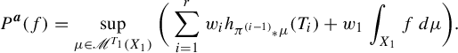
and established the variational principle [Reference Feng and HuangFH16, Theorem 1.4]:
$f:X_1 \rightarrow \mathbb {R}$
and established the variational principle [Reference Feng and HuangFH16, Theorem 1.4]:
 $$ \begin{align} P^{\boldsymbol{w}}_{\mathrm{FH}}(f) = \sup_{\mu \in \mathscr{M}^{T_1}(X_1)} \bigg( \sum_{i=1}^r w_i h_{{\pi^{(i-1)}}_*\mu} (T_i) + w_1 \int_{X_1} f\,d\mu \bigg). \end{align} $$
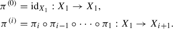
Here,
 $\pi ^{(i)}$
is defined by
$\pi ^{(i)}$
is defined by
 $$ \begin{gather*} \pi^{(0)} = \mathrm{id}_{X_1}: X_1 \to X_1, \\ \pi^{(i)} = \pi_i \circ \pi_{i-1} \circ \cdots \circ \pi_1: X_1 \to X_{i+1}, \end{gather*} $$
and
 ${\pi ^{(i-1)}}_* \mu $
is the push-forward measure of
${\pi ^{(i-1)}}_* \mu $
is the push-forward measure of
 $\mu $
by
$\mu $
by
 $\pi ^{(i-1)}$
on
$\pi ^{(i-1)}$
on
 $X_i$
. The
$X_i$
. The
 $\boldsymbol {w}$
-weighted topological entropy
$\boldsymbol {w}$
-weighted topological entropy
 $h^{\boldsymbol {w}}_{\mathrm {top}}(T_1)$
is the value of
$h^{\boldsymbol {w}}_{\mathrm {top}}(T_1)$
is the value of
 $P^{\boldsymbol {w}}_{\mathrm {FH}}(f)$
when
$P^{\boldsymbol {w}}_{\mathrm {FH}}(f)$
when
 $f \equiv 0$
. In this case, equation (1.2) becomes
$f \equiv 0$
. In this case, equation (1.2) becomes
 $$ \begin{align} h^{\boldsymbol{w}}_{\mathrm{top}}(T_1) = \sup_{\mu \in \mathscr{M}^{T_1}(X_1)} \bigg( \sum_{i=1}^r w_i h_{{\pi^{(i-1)}}_*\mu} (T_i) \bigg). \end{align} $$
We will explain here Feng and Huang’s method of defining
 $h^{\boldsymbol {w}}_{\mathrm {top}}(T_1)$
. For the definition of
$h^{\boldsymbol {w}}_{\mathrm {top}}(T_1)$
. For the definition of
 $P^{\boldsymbol {w}}_{\mathrm {FH}}(f)$
, see their original paper [Reference Feng and HuangFH16].
$P^{\boldsymbol {w}}_{\mathrm {FH}}(f)$
, see their original paper [Reference Feng and HuangFH16].
Let n be a natural number and
 $\varepsilon $
a positive number. Let
$\varepsilon $
a positive number. Let
 $d^{(i)}$
be a metric on
$d^{(i)}$
be a metric on
 $X_i$
. For
$X_i$
. For
 $x \in X_1$
, define the nth
$x \in X_1$
, define the nth
 $\boldsymbol {w}$
-weighted Bowen ball of radius
$\boldsymbol {w}$
-weighted Bowen ball of radius
 $\varepsilon $
centered at x by
$\varepsilon $
centered at x by
 $$ \begin{align*} B^{\boldsymbol{w}}_n(x, \varepsilon) = \bigg\{ y \in X_1 \bigg|\! \begin{array}{l} d^{(i)} \! ( T^j_i(\pi^{(i-1)}(x)), T^j_i(\pi^{(i-1)}(y))) < \varepsilon \text{ for every} \\ 0 \leq j \leq \left\lceil {(w_1 + \cdots + w_i)n} \right\rceil \text{ and } 1 \leq i \leq k. \end{array} \!\!\bigg\}. \end{align*} $$
Consider
 $\Gamma = \{ B^{\boldsymbol {w}}_{n_j}(x_j, \varepsilon ) \}_j$
, an at-most countable cover of
$\Gamma = \{ B^{\boldsymbol {w}}_{n_j}(x_j, \varepsilon ) \}_j$
, an at-most countable cover of
 $X_1$
by weighted Bowen balls. Let
$X_1$
by weighted Bowen balls. Let
 $n(\Gamma ) = \min _j n_j$
. For
$n(\Gamma ) = \min _j n_j$
. For
 $s \geq 0$
and
$s \geq 0$
and
 $N \in \mathbb {N}$
, let
$N \in \mathbb {N}$
, let
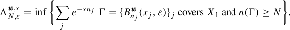 $$ \begin{align*} \Lambda^{\boldsymbol{w}, s}_{N, \varepsilon} = \inf \bigg\{\! \sum_j e^{-sn_j} \bigg| \Gamma = \{ B^{\boldsymbol{w}}_{n_j}(x_j, \varepsilon) \}_j \text{ covers } X_1 \text{ and } n(\Gamma) \geq N \bigg\}. \end{align*} $$
This quantity is non-decreasing as
 $N \to \infty $
. The following limit hence exists:
$N \to \infty $
. The following limit hence exists:
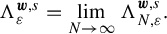 $$ \begin{align*} \Lambda^{\boldsymbol{w}, s}_{\varepsilon} = \lim_{N \to \infty} \Lambda^{\boldsymbol{w}, s}_{N, \varepsilon}. \end{align*} $$
There is a value of s where
 $\Lambda ^{\boldsymbol {w}, s}_{\varepsilon }$
jumps from
$\Lambda ^{\boldsymbol {w}, s}_{\varepsilon }$
jumps from
 $\infty $
to
$\infty $
to
 $0$
, which we will denote by
$0$
, which we will denote by
 $h^{\boldsymbol {w}}_{\mathrm {top}}(T_1, \varepsilon )$
:
$h^{\boldsymbol {w}}_{\mathrm {top}}(T_1, \varepsilon )$
:
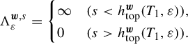 $$ \begin{align*} \Lambda^{\boldsymbol{w}, s}_{\varepsilon} = \begin{cases}\infty & (s < h^{\boldsymbol{w}}_{\mathrm{top}}(T_1, \varepsilon)), \\ 0 & (s> h^{\boldsymbol{w}}_{\mathrm{top}}(T_1, \varepsilon)). \end{cases} \end{align*} $$
The value
 $h^{\boldsymbol {w}}_{\mathrm {top}}(T_1, \varepsilon )$
is non-decreasing as
$h^{\boldsymbol {w}}_{\mathrm {top}}(T_1, \varepsilon )$
is non-decreasing as
 $\varepsilon \to 0$
. Therefore, we can define the
$\varepsilon \to 0$
. Therefore, we can define the
 $\boldsymbol {w}$
-weighted topological entropy
$\boldsymbol {w}$
-weighted topological entropy
 $h^{\boldsymbol {w}}_{\mathrm {top}}(T_1)$
by
$h^{\boldsymbol {w}}_{\mathrm {top}}(T_1)$
by
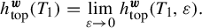 $$ \begin{align*} h^{\boldsymbol{w}}_{\mathrm{top}}(T_1) = \lim_{\varepsilon \to 0} h^{\boldsymbol{w}}_{\mathrm{top}}(T_1, \varepsilon). \end{align*} $$
An important point about this definition is that in some dynamical systems, such as self-affine sponges, the quantity
 $h^{\boldsymbol {w}}_{\mathrm {top}}(T_1)$
is directly related to the Hausdorff dimension of
$h^{\boldsymbol {w}}_{\mathrm {top}}(T_1)$
is directly related to the Hausdorff dimension of
 $X_1$
.
$X_1$
.
Example 1.1. Consider the self-affine sponges introduced in §1.2. Define
 $p_i: \mathbb {T}^{r-i+1} \rightarrow \mathbb {T}^{r-i}$
by
$p_i: \mathbb {T}^{r-i+1} \rightarrow \mathbb {T}^{r-i}$
by
 $$ \begin{align*} p_i(x_1, x_2, \ldots, x_{r-i}, x_{r-i+1}) = (x_1, x_2, \ldots, x_{r-i}). \end{align*} $$
Let
 $X_1 = K(T, D)$
,
$X_1 = K(T, D)$
,
 $X_i = p_{i-1} \circ p_i \circ \cdots \circ p_1(X_1)$
, and
$X_i = p_{i-1} \circ p_i \circ \cdots \circ p_1(X_1)$
, and
 $T_i: X_i \rightarrow X_i$
be the endomorphism defined by
$T_i: X_i \rightarrow X_i$
be the endomorphism defined by
 $A_i = \mathrm {diag}(m_1, m_2, \ldots , m_{r-i+1})$
. Define the factor maps
$A_i = \mathrm {diag}(m_1, m_2, \ldots , m_{r-i+1})$
. Define the factor maps
 $\pi _i: X_i \rightarrow X_{i+1}$
as the restrictions of
$\pi _i: X_i \rightarrow X_{i+1}$
as the restrictions of
 $p_i$
. Let
$p_i$
. Let
 $$ \begin{align} \boldsymbol{w} = \bigg( \frac{\log{m_1}}{\log{m_r}}, \quad \frac{\log{m_1}}{\log{m_{r-1}}} - \frac{\log{m_1}}{\log{m_r}}, \ldots , \quad \frac{\log{m_1}}{\log{m_2}} - \frac{\log{m_1}}{\log{m_3}}, \quad 1 - \frac{\log{m_1}}{\log{m_2}} \bigg). \end{align} $$
Then each nth
 $\boldsymbol {w}$
-weighted Bowen ball is approximately a square of side length
$\boldsymbol {w}$
-weighted Bowen ball is approximately a square of side length
 $\varepsilon m_1^{-n}$
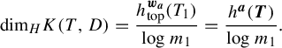
. Therefore,
$\varepsilon m_1^{-n}$
. Therefore,
 $$ \begin{align} \mathrm{dim}_H K(T, D) = \frac{h^{\boldsymbol{w}}_{\mathrm{top}}(T_1)}{\log{m_1}}. \end{align} $$
1.4. Tsukamoto’s approach and its extension
Following the work of Feng and Huang [Reference Feng and HuangFH16] described in §1.3, Tsukamoto [Reference TsukamotoTsu22] published an intriguing approach to these invariants. There, he gave a new definition of the weighted topological pressure for a factor map between two dynamical systems:
He then proved the variational principle using his definition, showing the surprising coincidence of the two definitions. His definition of weighted topological entropy allowed for relatively easy calculations for sets like self-affine carpets.
We will extend Tsukamoto’s idea, redefine the weighted topological pressure for a sequence of dynamical systems of arbitrary length, and establish the variational principle. Here we will explain our definition in the case
 $f \equiv 0$
. See §2 for the general setting. We will not explain Tsukamoto’s definition itself since it is obtained by letting
$f \equiv 0$
. See §2 for the general setting. We will not explain Tsukamoto’s definition itself since it is obtained by letting
 $r=2$
in the following argument.
$r=2$
in the following argument.
Consider a sequence of dynamical systems:
Take a metric
 $d^{(i)}$
on
$d^{(i)}$
on
 $X_i$
. Let
$X_i$
. Let
 ${\boldsymbol {a}}=(a_1, a_2, \ldots , a_{r-1})$
with
${\boldsymbol {a}}=(a_1, a_2, \ldots , a_{r-1})$
with
 $0 \leq a_i \leq 1$
for each i. Let N be a natural number and
$0 \leq a_i \leq 1$
for each i. Let N be a natural number and
 $\varepsilon $
a positive number. We define a new metric
$\varepsilon $
a positive number. We define a new metric
 $d^{(i)}_N$
on
$d^{(i)}_N$
on
 $X_i$
by
$X_i$
by
 $$ \begin{align*} d^{(i)}_N(x_1, x_2) = \max_{0\leq n < N} d^{(i)}({T_i}^n x_1, {T_i}^n x_2). \end{align*} $$
We inductively define a quantity
 $\#^{\boldsymbol {a}}_i(\Omega , N, \varepsilon )$
for
$\#^{\boldsymbol {a}}_i(\Omega , N, \varepsilon )$
for
 $\Omega \subset X_i$
. For
$\Omega \subset X_i$
. For
 $\Omega \subset X_1$
, set
$\Omega \subset X_1$
, set
 $$ \begin{align*} \#^{\boldsymbol{a}}_1(\Omega, N, \varepsilon) &= \min \bigg\{ n \in \mathbb{N} \bigg|\! \begin{array}{l} \text{There exists an open cover } \{U_j\}_{j=1}^n \text{ of } \Omega \\ \text{with } \mathrm{diam}(U_j, d_N^{(1)}) < \varepsilon \text{ for all } 1 \leq j \leq n \end{array}\!\!\bigg\}. \end{align*} $$
(The quantity
 $\#^{\boldsymbol {a}}_1(\Omega , N, \varepsilon )$
is independent of the parameter
$\#^{\boldsymbol {a}}_1(\Omega , N, \varepsilon )$
is independent of the parameter
 $\boldsymbol {a}$
. However, we use this notation for the convenience of what follows.) Let
$\boldsymbol {a}$
. However, we use this notation for the convenience of what follows.) Let
 $\Omega \subset X_{i+1}$
. Suppose
$\Omega \subset X_{i+1}$
. Suppose
 $\#^{\boldsymbol {a}}_i$
is already defined. We set
$\#^{\boldsymbol {a}}_i$
is already defined. We set
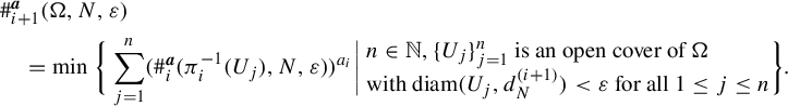 $$ \begin{align*} & \#^{\boldsymbol{a}}_{i+1}(\Omega, N, \varepsilon)\\&\quad = \min \bigg\{ \sum_{j=1}^n ( \#^{\boldsymbol{a}}_i(\pi_i^{-1}(U_j), N, \varepsilon) )^{a_i} \bigg|\! \begin{array}{l} n \in \mathbb{N}, \{U_j\}_{j=1}^n \text{ is an open cover of } \Omega \\ \text{with } \mathrm{diam}(U_j, d_N^{(i+1)}) < \varepsilon \text{ for all } 1 \leq j \leq n \end{array} \!\!\bigg\}. \end{align*} $$
We define the topological entropy of
 ${\boldsymbol {a}}$
-exponent
${\boldsymbol {a}}$
-exponent
 $h^{\boldsymbol {a}}(\boldsymbol {T})$
, where
$h^{\boldsymbol {a}}(\boldsymbol {T})$
, where
 $\boldsymbol {T} = (T_i)_i$
, by
$\boldsymbol {T} = (T_i)_i$
, by
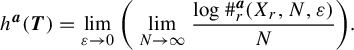 $$ \begin{align*} h^{\boldsymbol{a}}(\boldsymbol{T}) = \lim_{\varepsilon \to 0} \bigg( \lim_{N \to \infty} \frac{\log{\#^{\boldsymbol{a}}_r(X_r, N, \varepsilon)}}{N} \bigg). \end{align*} $$
This limit exists since
 $\log {\#^{\boldsymbol {a}}_r(X_r, N, \varepsilon )}$
is sub-additive in N and non-decreasing as
$\log {\#^{\boldsymbol {a}}_r(X_r, N, \varepsilon )}$
is sub-additive in N and non-decreasing as
 $\varepsilon $
tends to
$\varepsilon $
tends to
 $0$
.
$0$
.
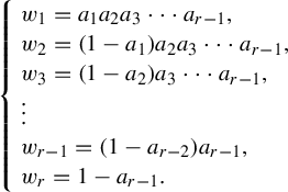
From
 ${\boldsymbol {a}}=(a_1, a_2, \ldots , a_{r-1})$
, we define a probability vector (that is, all entries are non-negative, and their sum is 1)
${\boldsymbol {a}}=(a_1, a_2, \ldots , a_{r-1})$
, we define a probability vector (that is, all entries are non-negative, and their sum is 1)
 $\boldsymbol {w_a} = (w_1, \ldots , w_r)$
by
$\boldsymbol {w_a} = (w_1, \ldots , w_r)$
by
 $$ \begin{align*} \left\{\! \begin{array}{l} w_1 = a_1 a_2 a_3 \cdots a_{r-1},\\ w_2 = (1-a_1) a_2 a_3 \cdots a_{r-1}, \\ w_3 = (1-a_2) a_3 \cdots a_{r-1}, \\ \vdots \\ w_{r-1} = (1-a_{r-2}) a_{r-1}, \\ w_r = 1- a_{r-1}. \end{array} \right.\!\! \end{align*} $$
The following theorem is a direct consequence of our main result in Theorem 2.1.
Theorem 1.2. For
 ${\boldsymbol {a}}=(a_1, a_2, \ldots , a_{r-1})$
with
${\boldsymbol {a}}=(a_1, a_2, \ldots , a_{r-1})$
with
 $0 \leq a_i \leq 1$
for each i,
$0 \leq a_i \leq 1$
for each i,
 $$ \begin{align} h^{\boldsymbol{a}}(\boldsymbol{T}) = \sup_{\mu \in \mathscr{M}^{T_1}(X_1)} \bigg( \sum_{i=1}^r w_i h_{{\pi^{(i-1)}}_*\mu} (T_i) \bigg). \end{align} $$
The strategy of the proof is adopted from Tsukamoto’s paper. However, there are some additional difficulties. Let
 $h^{\boldsymbol {a}}_{\mathrm {var}}(\boldsymbol {T})$
be the right-hand side of equation (1.6). We use the ‘zero-dimensional trick’ for proving
$h^{\boldsymbol {a}}_{\mathrm {var}}(\boldsymbol {T})$
be the right-hand side of equation (1.6). We use the ‘zero-dimensional trick’ for proving
 $h^{\boldsymbol {a}}(\boldsymbol {T}) \leq h^{\boldsymbol {a}}_{\mathrm {var}}(\boldsymbol {T})$
, meaning we reduce the proof to the case where all dynamical systems are zero-dimensional. Merely taking a zero-dimensional extension for each
$h^{\boldsymbol {a}}(\boldsymbol {T}) \leq h^{\boldsymbol {a}}_{\mathrm {var}}(\boldsymbol {T})$
, meaning we reduce the proof to the case where all dynamical systems are zero-dimensional. Merely taking a zero-dimensional extension for each
 $X_i$
does not work. Therefore, we realize this by taking step by step extensions of the whole sequence of dynamical systems (see §3.3). Then we show
$X_i$
does not work. Therefore, we realize this by taking step by step extensions of the whole sequence of dynamical systems (see §3.3). Then we show
 $h^{\boldsymbol {a}}(\boldsymbol {T}) \leq h^{\boldsymbol {a}}_{\mathrm {var}}(\boldsymbol {T})$
by using an appropriate measure, the definition of which is quite sophisticated (see
$h^{\boldsymbol {a}}(\boldsymbol {T}) \leq h^{\boldsymbol {a}}_{\mathrm {var}}(\boldsymbol {T})$
by using an appropriate measure, the definition of which is quite sophisticated (see
 $\sigma _N$
in the proof of Theorem 4.1). In proving
$\sigma _N$
in the proof of Theorem 4.1). In proving
 $h^{\boldsymbol {a}}(\boldsymbol {T}) \geq h^{\boldsymbol {a}}_{\mathrm {var}}(\boldsymbol {T})$
, the zero-dimensional trick can not be used. The proof, therefore, requires a detailed estimation of these quantities for arbitrary covers, which is more complicated than the original argument in [Reference TsukamotoTsu22].
$h^{\boldsymbol {a}}(\boldsymbol {T}) \geq h^{\boldsymbol {a}}_{\mathrm {var}}(\boldsymbol {T})$
, the zero-dimensional trick can not be used. The proof, therefore, requires a detailed estimation of these quantities for arbitrary covers, which is more complicated than the original argument in [Reference TsukamotoTsu22].
Theorem 1.2 and Feng and Huang’s version of variational principle in equation (1.3) yield the following corollary.
Corollary 1.3. For
 ${\boldsymbol {a}}=(a_1, a_2, \ldots , a_{r-1})$
with
${\boldsymbol {a}}=(a_1, a_2, \ldots , a_{r-1})$
with
 $0 < a_i \leq 1$
for each i,
$0 < a_i \leq 1$
for each i,
 $$ \begin{align*} h^{\boldsymbol{a}}(\boldsymbol{T}) = h^{\boldsymbol{w_a}}_{\mathrm{top}}(T_1). \end{align*} $$
This corollary is rather profound, connecting the two seemingly different quantities. We can calculate the Hausdorff dimension of self-affine sponges using this result as in the following example. Additionally, we will show in §6 that we can now determine the Hausdorff dimension of certain sofic sets in higher-dimensional Euclidean space.
Example 1.4. Let us take another look at self-affine sponges. Kenyon and Peres [Reference Kenyon and PeresKP96, Theorem 1.2] calculated their Hausdorff dimension as follows. Recall the notation in §1.2 and that
 $m_1 \leq m_2 \leq \cdots \leq m_r$
.
$m_1 \leq m_2 \leq \cdots \leq m_r$
.
Theorem 1.5. Define a sequence of real numbers
 $(Z_j)_j$
as follows. Let
$(Z_j)_j$
as follows. Let
 $Z_r$
be the indicator of D, namely,
$Z_r$
be the indicator of D, namely,
 $Z_r(i_1, \ldots , i_r) = 1$
if
$Z_r(i_1, \ldots , i_r) = 1$
if
 $(i_1, \ldots , i_r) \in D$
and
$(i_1, \ldots , i_r) \in D$
and
 $0$
otherwise. Define
$0$
otherwise. Define
 $Z_{r-1}$
by
$Z_{r-1}$
by
 $$ \begin{align*} Z_{r-1}(i_1, \ldots, i_{r-1}) = \sum_{i_r = 0}^{m_r-1} Z_r(i_1, \ldots, i_{r-1}, i_r). \end{align*} $$
More generally, if
 $Z_{j+1}$
is already defined, let
$Z_{j+1}$
is already defined, let
 $$ \begin{align*} Z_j(i_1, \ldots, i_j) = \sum_{i_{j+1} = 0}^{m_{j+1}-1} Z_{j+1}(i_1, \ldots, i_j, i_{j+1})^{\log{m_{j+1}}/\log{m_{j+2}}}. \end{align*} $$
Then
 $$ \begin{align*} \mathrm{dim}_H K(T, D) = \frac{\log{Z_0}}{\log{m_1}}. \end{align*} $$
We can prove this result in a fairly elementary way by Corollary 1.3 without requiring measure theory on the surface. Set
 $a_i = \log _{m_{r-i+1}} m_{r-i}$
for each
$a_i = \log _{m_{r-i+1}} m_{r-i}$
for each
 $1 \leq i \leq r-1$
, then
$1 \leq i \leq r-1$
, then
 $\boldsymbol {w_a}$
equals
$\boldsymbol {w_a}$
equals
 $\boldsymbol {w}$
in equation (1.4). Combining equation (1.5) and Corollary 1.3, we have
$\boldsymbol {w}$
in equation (1.4). Combining equation (1.5) and Corollary 1.3, we have
 $$ \begin{align*} \mathrm{dim}_H K(T, D) = \frac{h^{\boldsymbol{w_a}}_{\mathrm{top}}(T_1)}{\log{m_1}} = \frac{h^{\boldsymbol{a}}(\boldsymbol{T})}{\log{m_1}}. \end{align*} $$
Hence, we need to show the following claim.
Claim 1.6. We have
 $$ \begin{align*} h^{\boldsymbol{a}}(\boldsymbol{T}) = \log{Z_0}. \end{align*} $$
Proof. Observe first that taking the infimum over closed covers instead of open ones in the definition of
 $h^{\boldsymbol {a}}(\boldsymbol {T})$
does not change its value. Define a metric
$h^{\boldsymbol {a}}(\boldsymbol {T})$
does not change its value. Define a metric
 $d^{(i)}$
on each
$d^{(i)}$
on each
 $X_i$
by
$X_i$
by
 $$ \begin{align*} d^{(i)} (x, y) = \min_{n \in {\mathbb{Z}}^{r-i+1}} \left\lvert {x-y-n} \right\rvert. \end{align*} $$
Let
 $$ \begin{align*} D_j = \{ (e_1, \ldots, e_j) | \text{ there are } e_{j+1}, \ldots, e_r \text{ with } (e_1, \ldots, e_r) \in D \}. \end{align*} $$
Define
 $p_i: D_{r-i+1} \rightarrow D_{r-i}$
by
$p_i: D_{r-i+1} \rightarrow D_{r-i}$
by
 $p_i(e_1, \ldots , e_{r-i+1}) = (e_1, \ldots , e_{r-i})$
. Fix
$p_i(e_1, \ldots , e_{r-i+1}) = (e_1, \ldots , e_{r-i})$
. Fix
 $0 < \varepsilon < {1}/{m_r}$
and take a natural number n with
$0 < \varepsilon < {1}/{m_r}$
and take a natural number n with
 $m_1^{-n} < \varepsilon $
. Fix a natural number N and let
$m_1^{-n} < \varepsilon $
. Fix a natural number N and let
 $\psi _i: D_{r-i+1}^{N+n} \rightarrow D_{r-i}^{N+n}$
be the product map of
$\psi _i: D_{r-i+1}^{N+n} \rightarrow D_{r-i}^{N+n}$
be the product map of
 $p_i$
, that is,
$p_i$
, that is,
 $\psi _i(v_1, \ldots , v_{N+n}) = (p_i(v_1), \ldots , p_i(v_{N+n}))$
.
$\psi _i(v_1, \ldots , v_{N+n}) = (p_i(v_1), \ldots , p_i(v_{N+n}))$
.
For
 $x \in D_{r-i+1}^{N+n}$
, define (recall that
$x \in D_{r-i+1}^{N+n}$
, define (recall that
 $A_i = \mathrm {diag}(m_1, m_2, \ldots , m_{r-i+1})$
)
$A_i = \mathrm {diag}(m_1, m_2, \ldots , m_{r-i+1})$
)
 $$ \begin{align*} U^{(i)}_x = \bigg\{ \sum_{k=0}^{\infty} A_i^{-k} e_k \in X_i \bigg| e_k \in D_{r-i+1} \text{ for each } k \text{ and } (e_1, \ldots, e_{N+n}) = x \bigg\}. \end{align*} $$
Then
 $\{U^{(i)}_x\}_{x \in D^{N+n}_{r-i+1}}$
is a closed cover of
$\{U^{(i)}_x\}_{x \in D^{N+n}_{r-i+1}}$
is a closed cover of
 $X_i$
with
$X_i$
with
 $\mathrm {diam}(U^{(i)}_x, d^{(i)}_N) < \varepsilon $
. For
$\mathrm {diam}(U^{(i)}_x, d^{(i)}_N) < \varepsilon $
. For
 $x, y \in D^{N+n}_{r-i+1}$
, we write
$x, y \in D^{N+n}_{r-i+1}$
, we write
 $x \backsim y$
if and only if
$x \backsim y$
if and only if
 $U^{(i)}_x \cap U^{(i)}_y \ne \varnothing $
. We have for any i and
$U^{(i)}_x \cap U^{(i)}_y \ne \varnothing $
. We have for any i and
 $x \in D_{r-i}^{N+n}$
,
$x \in D_{r-i}^{N+n}$
,
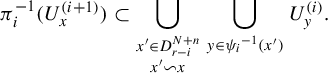 $$ \begin{align*} \pi_i^{-1}(U^{(i+1)}_x) \subset \bigcup_{\substack{x' \in D_{r-i}^{N+n} \\ x' \backsim x}} \bigcup_{y \in {\psi_i}^{-1}(x')} U^{(i)}_y. \end{align*} $$
Notice that for each
 $x \in D_{r-i}^{N+n}$
, the number of
$x \in D_{r-i}^{N+n}$
, the number of
 $x' \in D_{r-i}^{N+n}$
with
$x' \in D_{r-i}^{N+n}$
with
 $x' \backsim x$
is not more than
$x' \backsim x$
is not more than
 $3^r$
. Therefore, for every
$3^r$
. Therefore, for every
 $v = (v_1^{(1)}, \ldots , v_{N+n}^{(1)}) \in D_{r-1}^{N+n}$
, there are
$v = (v_1^{(1)}, \ldots , v_{N+n}^{(1)}) \in D_{r-1}^{N+n}$
, there are
 $(v_1^{(k)}, \ldots , v_{N+n}^{(k)}) \in D_{r-1}^{N+n}$
,
$(v_1^{(k)}, \ldots , v_{N+n}^{(k)}) \in D_{r-1}^{N+n}$
,
 $k = 2, 3, \ldots , L$
, and
$k = 2, 3, \ldots , L$
, and
 $L \leq 3^r$
, with
$L \leq 3^r$
, with
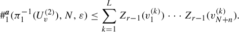 $$ \begin{align*} \#^{\boldsymbol{a}}_1(\pi_1^{-1}(U^{(2)}_v), N, \varepsilon) \leq \sum_{k=1}^L Z_{r-1}(v_1^{(k)})\cdots Z_{r-1}(v_{N+n}^{(k)}). \end{align*} $$
We inductively continue while considering that the multiplicity is at most
 $3^r$
and obtain
$3^r$
and obtain
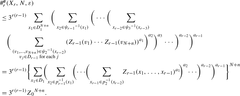 $$ \begin{align*} & \#^{\boldsymbol{a}}_r(X_r, N, \varepsilon) \\&\leq 3^{r(r-1)} \sum_{x_1 \in D^{N+n}_1}\bigg( \sum_{x_2 \in {\psi_{r-1}}^{-1}(x_1)} \bigg( \cdots \bigg( \sum_{x_{r-2} \in {\psi_3}^{-1}(x_{r-3})} \\&\quad\bigg( \sum_{\substack{(v_1, \ldots, v_{N+n}) \in {\psi_2}^{-1}(x_{r-2}) \\ v_j \in D_{r-1} \text{ for each } j }} ( Z_{r-1}(v_1)\cdots Z_{r-1}(v_{N+n}))^{a_1} \bigg)^{a_2} \bigg)^{a_3} \cdots \bigg)^{a_{r-2}}\bigg)^{a_{r-1}}\\&= 3^{r(r-1)} \bigg\{\! \sum_{x_1 \in D_1}\!\! \bigg(\! \sum_{x_2 \in p_{r-1}^{-1}(x_1)}\!\! \bigg(\! \cdots \!\bigg(\! \sum_{x_{r-1} \in p_2^{-1}(x_{r-2})}\!\! {Z_{r-1}(x_1, \ldots, x_{r-1})}^{a_1} \!\bigg)^{a_2}\!\cdots\! \bigg)^{a_{r-2}}\bigg)^{a_{r-1}} \bigg\}^{N+n} \\&= 3^{r(r-1)} {Z_0}^{N+n}. \end{align*} $$
Therefore,
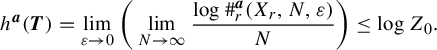 $$ \begin{align*} h^{\boldsymbol{a}}(\boldsymbol{T}) = \lim_{\varepsilon \to 0} \bigg( \lim_{N \to \infty} \frac{\log{\#^{\boldsymbol{a}}_r(X_r, N, \varepsilon)}}{N} \bigg) \leq \log{Z_0}. \end{align*} $$
Next, we prove
 $h^{\boldsymbol {a}}(\boldsymbol {T}) \geq \log {Z_0}$
. We fix
$h^{\boldsymbol {a}}(\boldsymbol {T}) \geq \log {Z_0}$
. We fix
 $0 < \varepsilon < {1}/{m_r}$
and use
$0 < \varepsilon < {1}/{m_r}$
and use
 $\varepsilon $
-separated sets. Take and fix
$\varepsilon $
-separated sets. Take and fix
 $\boldsymbol {s} = (t_1, \ldots , t_r) \in D$
, and set
$\boldsymbol {s} = (t_1, \ldots , t_r) \in D$
, and set
 $\boldsymbol {s}_i = (t_1, \ldots , t_{r-i+1})$
. Fix a natural number N and let
$\boldsymbol {s}_i = (t_1, \ldots , t_{r-i+1})$
. Fix a natural number N and let
 $\psi _i: D_{r-i+1}^N \rightarrow D_{r-i}^N$
be the product map of
$\psi _i: D_{r-i+1}^N \rightarrow D_{r-i}^N$
be the product map of
 $p_i$
as in the previous definition. Define
$p_i$
as in the previous definition. Define
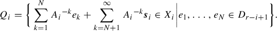 $$ \begin{align*} Q_i = \bigg\{ \sum_{k=1}^N {A_i}^{-k} e_k + \sum_{k=N+1}^{\infty} {A_i}^{-k} \boldsymbol{s}_i \in X_i \bigg| e_1, \ldots, e_N \in D_{r-i+1} \bigg\}. \end{align*} $$
Then
 $Q_i$
is an
$Q_i$
is an
 $\varepsilon $
-separated set with respect to the metric
$\varepsilon $
-separated set with respect to the metric
 $d^{(i)}_N$
on
$d^{(i)}_N$
on
 $X_i$
. Consider an arbitrary open cover
$X_i$
. Consider an arbitrary open cover
 $\mathscr {F}^{(i)}$
of
$\mathscr {F}^{(i)}$
of
 $X_i$
for each i with the following properties (this
$X_i$
for each i with the following properties (this
 $(\mathscr {F}^{(i)})_i$
is defined as a chain of open (N,
$(\mathscr {F}^{(i)})_i$
is defined as a chain of open (N,
 $\varepsilon $
)-covers of
$\varepsilon $
)-covers of
 $(X_i)_i$
in Definition 3.1).
$(X_i)_i$
in Definition 3.1).
-
(1) For every i and
 $V \in \mathscr {F}^{(i)}$
, we have
$\mathrm {diam}(V, d^{(i)}_N) < \varepsilon $
.
$V \in \mathscr {F}^{(i)}$
, we have
$\mathrm {diam}(V, d^{(i)}_N) < \varepsilon $
. -
(2) For each
$1 \leq i \leq r-1$
and
$U \in \mathscr {F}^{(i+1)}$
, there is
$\mathscr {F}^{(i)}(U) \subset \mathscr {F}^{(i)}$
such that and
$$ \begin{align*} \pi_i^{-1}(U) \subset \bigcup \mathscr{F}^{(i)}(U) \end{align*} $$
$$ \begin{align*} \mathscr{F}^{(i)} = \bigcup_{U \in \mathscr{F}^{(i+1)}} \mathscr{F}^{(i)}(U). \end{align*} $$


We have
 $\#(V \cap Q_i ) \leq 1$
for each
$\#(V \cap Q_i ) \leq 1$
for each
 $V \in \mathscr {F}^{(i)}$
by (1). Let
$V \in \mathscr {F}^{(i)}$
by (1). Let
 $(e^{(2)}_1, e^{(2)}_2, \ldots , e^{(2)}_N) \in D_{r-1}^N$
and suppose
$(e^{(2)}_1, e^{(2)}_2, \ldots , e^{(2)}_N) \in D_{r-1}^N$
and suppose
 $U \in \mathscr {F}^{(2)}$
satisfies
$U \in \mathscr {F}^{(2)}$
satisfies
 $$ \begin{align*} \sum_{k=1}^N {A_2}^{-k} e^{(2)}_k + \sum_{k=N+1}^{\infty} {A_2}^{-k} \boldsymbol{s}_2 \in U \cap Q_2. \end{align*} $$
Then
 $\pi _1^{-1}(U)$
contains at least
$\pi _1^{-1}(U)$
contains at least
 $Z_{r-1}(e^{(2)}_1)\cdots Z_{r-1}(e^{(2)}_N)$
points of
$Z_{r-1}(e^{(2)}_1)\cdots Z_{r-1}(e^{(2)}_N)$
points of
 $Q_1$
. Hence,
$Q_1$
. Hence,
 $$ \begin{align*} \#^{\boldsymbol{a}}_1(\pi_1^{-1}(U), N, \varepsilon)\geq Z_{r-1}(e^{(2)}_1)\cdots Z_{r-1}(e^{(2)}_N). \end{align*} $$
We continue this reasoning inductively and get
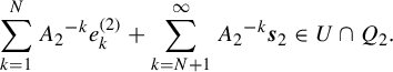
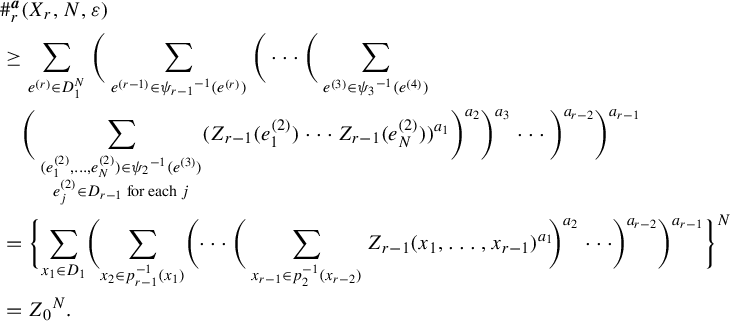 $$ \begin{align*} & \#^{\boldsymbol{a}}_r(X_r, N, \varepsilon) \\&\geq \sum_{e^{(r)} \in D^N_1}\bigg( \sum_{e^{(r-1)} \in {\psi_{r-1}}^{-1}(e^{(r)})} \bigg( \cdots \bigg( \sum_{e^{(3)} \in {\psi_3}^{-1}(e^{(4)})} \\&\quad\bigg( \sum_{\substack{(e^{(2)}_1, \ldots, e^{(2)}_N) \in {\psi_2}^{-1}(e^{(3)}) \\ e^{(2)}_j \in D_{r-1} \text{ for each } j }} ( Z_{r-1}(e^{(2)}_1)\cdots Z_{r-1}(e^{(2)}_N))^{a_1} \bigg)^{a_2} \bigg)^{a_3} \cdots \bigg)^{a_{r-2}}\bigg)^{a_{r-1}}\\&= \bigg\{\! \sum_{x_1 \in D_1} \!\bigg(\! \sum_{x_2 \in p_{r-1}^{-1}(x_1)} \!\bigg(\! \cdots \bigg( \sum_{x_{r-1} \in p_2^{-1}(x_{r-2})} {Z_{r-1}(x_1, \ldots, x_{r-1})}^{a_1} \!\bigg)^{a_2} \cdots \!\bigg)^{a_{r-2}}\bigg)^{a_{r-1}} \bigg\}^N \\&= {Z_0}^N. \end{align*} $$
This implies
 $$ \begin{align*} h^{\boldsymbol{a}}(\boldsymbol{T}) \geq \log{Z_0}. \end{align*} $$
We conclude that
 $$ \begin{align*} h^{\boldsymbol{a}}(\boldsymbol{T}) = \log{Z_0}.\\[-34pt] \end{align*} $$
We would like to mention the work of Barral and Feng [Reference Barral and FengBF12, Reference FengFe11], and of Yayama [Reference YayamaYa11]. These papers studied the related invariants when
 $(X_i, T_i) (i =1, \ldots , r)$
are subshifts over finite alphabets. In this subshift case, our definition of
$(X_i, T_i) (i =1, \ldots , r)$
are subshifts over finite alphabets. In this subshift case, our definition of
 $h^{\boldsymbol {a}}(\boldsymbol {T})$
(and its pressure version in §2) is essentially the same as that given in [Reference Barral and FengBF12, Theorem 3.1]. Hence, we can say that our definition generalizes the approach in [Reference Barral and FengBF12, Theorem 3.1] from subshifts to general dynamical systems.
$h^{\boldsymbol {a}}(\boldsymbol {T})$
(and its pressure version in §2) is essentially the same as that given in [Reference Barral and FengBF12, Theorem 3.1]. Hence, we can say that our definition generalizes the approach in [Reference Barral and FengBF12, Theorem 3.1] from subshifts to general dynamical systems.
2. Weighted topological pressure
Here, we introduce the generalized, new definition of weighted topological pressure. Let
 $(X_i, T_i)$
(
$(X_i, T_i)$
(
 $i\hspace{-1pt}=\hspace{-1pt}1, 2, \ldots , r$
) be dynamical systems and
$i\hspace{-1pt}=\hspace{-1pt}1, 2, \ldots , r$
) be dynamical systems and
 $\pi _i: X_i\hspace{-1pt} \rightarrow\hspace{-1pt} X_{i+1}\, (i\hspace{-1pt}=\hspace{-1pt}1, 2, \ldots , r\hspace{-1pt}-\hspace{-1pt}1)$
factor maps. For a continuous function
$\pi _i: X_i\hspace{-1pt} \rightarrow\hspace{-1pt} X_{i+1}\, (i\hspace{-1pt}=\hspace{-1pt}1, 2, \ldots , r\hspace{-1pt}-\hspace{-1pt}1)$
factor maps. For a continuous function
 $f: X_1 \to \mathbb {R}$
and a natural number N, set
$f: X_1 \to \mathbb {R}$
and a natural number N, set
 $$ \begin{align*} S_N f (x) = f(x) + f(T_1 x) + f(T_1^2 x) + \cdots + f(T_1^{N-1}x). \end{align*} $$
Let
 $d^{(i)}$
be a metric on
$d^{(i)}$
be a metric on
 $X_i$
. Recall that we defined a new metric
$X_i$
. Recall that we defined a new metric
 $d^{(i)}_N$
on
$d^{(i)}_N$
on
 $X_i$
by
$X_i$
by
 $$ \begin{align*} d^{(i)}_N(x_1, x_2) = \max_{0\leq n < N} d^{(i)}({T_i}^n x_1, {T_i}^n x_2). \end{align*} $$
We may write these as
 $S_N^{T_1}f$
or
$S_N^{T_1}f$
or
 $d^{T_i}_N$
to clarify the maps
$d^{T_i}_N$
to clarify the maps
 $T_1$
and
$T_1$
and
 $T_i$
in the definitions above.
$T_i$
in the definitions above.
Let
 ${\boldsymbol {a}}=(a_1, a_2, \ldots , a_{r-1})$
with
${\boldsymbol {a}}=(a_1, a_2, \ldots , a_{r-1})$
with
 $0 \leq a_i \leq 1$
for each i and
$0 \leq a_i \leq 1$
for each i and
 $\varepsilon $
a positive number. We inductively define a quantity
$\varepsilon $
a positive number. We inductively define a quantity
 $P^{\boldsymbol {a}}_i(\Omega , f, N, \varepsilon )$
for
$P^{\boldsymbol {a}}_i(\Omega , f, N, \varepsilon )$
for
 $\Omega \subset X_i$
. For
$\Omega \subset X_i$
. For
 $\Omega \subset X_1$
, set
$\Omega \subset X_1$
, set
 $$ \begin{align*} & P^{\boldsymbol{a}}_1(\Omega, f, N, \varepsilon)\\ &\quad = \inf \bigg\{\sum_{j=1}^n \exp ( \sup_{U_j} S_N f) \bigg|\! \begin{array}{l} n \in \mathbb{N}, \{U_j\}_{j=1}^n \text{ is an open cover of } \Omega \\ \text{with } \mathrm{diam}(U_j, d_N^{(1)}) < \varepsilon \text{ for all } 1 \leq j \leq n \end{array} \!\!\bigg\}. \end{align*} $$
Let
 $\Omega \subset X_{i+1}$
. If
$\Omega \subset X_{i+1}$
. If
 $P^{\boldsymbol {a}}_i$
is already defined, let
$P^{\boldsymbol {a}}_i$
is already defined, let
 $$ \begin{align*} & P^{\boldsymbol{a}}_{i+1}(\Omega, f, N, \varepsilon) \\&\quad= \inf \bigg\{ \sum_{j=1}^n ( P^{\boldsymbol{a}}_i(\pi_i^{-1}(U_j), f, N, \varepsilon))^{a_i} \bigg|\! \begin{array}{l} n \in \mathbb{N}, \{U_j\}_{j=1}^n \text{ is an open cover of } \Omega \\ \text{with } \mathrm{diam}(U_j, d_N^{T_{i+1}}) < \varepsilon \text{ for all } 1 \leq j \leq n \end{array} \!\!\bigg\}. \end{align*} $$
We define the topological pressure of
 ${\boldsymbol {a}}$
-exponent
${\boldsymbol {a}}$
-exponent
 $P^{\boldsymbol {a}}(f)$
by
$P^{\boldsymbol {a}}(f)$
by
 $$ \begin{align*} P^{\boldsymbol{a}}(f) = \lim_{\varepsilon \to 0} \bigg( \lim_{N \to \infty} \frac{\log{P^{\boldsymbol{a}}_r(X_r, f, N, \varepsilon)}}{N} \bigg). \end{align*} $$
This limit exists since
 $\log {P^{\boldsymbol {a}}_r(X_r, f, N, \varepsilon )}$
is sub-additive in N and non-decreasing as
$\log {P^{\boldsymbol {a}}_r(X_r, f, N, \varepsilon )}$
is sub-additive in N and non-decreasing as
 $\varepsilon $
tends to
$\varepsilon $
tends to
 $0$
. When
$0$
. When
 $r=1$
, this coincides with the standard definition of the topological pressure
$r=1$
, this coincides with the standard definition of the topological pressure
 $P(f)$
on
$P(f)$
on
 $(X_1, T_1)$
. The topological entropy
$(X_1, T_1)$
. The topological entropy
 $h_{\mathrm {top}}(T_1)$
is the value of
$h_{\mathrm {top}}(T_1)$
is the value of
 $P(f)$
when
$P(f)$
when
 $f \equiv 0$
. When we want to clarify the maps
$f \equiv 0$
. When we want to clarify the maps
 $T_i$
and
$T_i$
and
 $\pi _i$
used in the definition of
$\pi _i$
used in the definition of
 $P^{\boldsymbol {a}}(f)$
, we will denote it by
$P^{\boldsymbol {a}}(f)$
, we will denote it by
 $P^{\boldsymbol {a}}(f, \boldsymbol {T})$
or
$P^{\boldsymbol {a}}(f, \boldsymbol {T})$
or
 $P^{\boldsymbol {a}}(f, \boldsymbol {T}, \boldsymbol {\pi })$
with
$P^{\boldsymbol {a}}(f, \boldsymbol {T}, \boldsymbol {\pi })$
with
 $\boldsymbol {T}=(T_i)_{i=1}^r$
and
$\boldsymbol {T}=(T_i)_{i=1}^r$
and
 $\boldsymbol {\pi } = (\pi _i)_{i=1}^r$
.
$\boldsymbol {\pi } = (\pi _i)_{i=1}^r$
.
Recall that we defined a probability vector
 $\boldsymbol {w_a} = (w_1, \ldots , w_r)$
from
$\boldsymbol {w_a} = (w_1, \ldots , w_r)$
from
 ${\boldsymbol {a}}=(a_1, a_2, \ldots , a_{r-1})$
by
${\boldsymbol {a}}=(a_1, a_2, \ldots , a_{r-1})$
by
 $$ \begin{align} \left\{\! \begin{array}{l} w_1 = a_1 a_2 a_3 \cdots a_{r-1},\\ w_2 = (1-a_1) a_2 a_3 \cdots a_{r-1}, \\ w_3 = (1-a_2) a_3 \cdots a_{r-1}, \\ \vdots \\ w_{r-1} = (1-a_{r-2}) a_{r-1}, \\ w_r = 1- a_{r-1}. \end{array} \right.\!\! \end{align} $$
Let
 $$ \begin{align*} \pi^{(0)} &= \mathrm{id}_{X_1}: X_1 \to X_1, \\ \pi^{(i)} &= \pi_i \circ \pi_{i-1} \circ \cdots \circ \pi_1: X_1 \to X_{i+1}. \end{align*} $$
We can now state the main result of this paper.
Theorem 2.1. Let
 $(X_i, T_i)$
(
$(X_i, T_i)$
(
 $i=1, 2, \ldots , r$
) be dynamical systems and
$i=1, 2, \ldots , r$
) be dynamical systems and
 $\pi _i: X_i \rightarrow X_{i+1}\ (i=1, 2, \ldots , r-1)$
factor maps. For any continuous function
$\pi _i: X_i \rightarrow X_{i+1}\ (i=1, 2, \ldots , r-1)$
factor maps. For any continuous function
 $f: X_1 \to \mathbb {R}$
,
$f: X_1 \to \mathbb {R}$
,
 $$ \begin{align} P^{\boldsymbol{a}}(f) = \sup_{\mu \in \mathscr{M}^{T_1}(X_1)} \bigg( \sum_{i=1}^r w_i h_{{\pi^{(i-1)}}_*\mu} (T_i) + w_1 \int_{X_1} f\,d\mu \bigg). \end{align} $$
We define
 $P^{\boldsymbol {a}}_{\mathrm {var}}(f)$
to be the right-hand side of this equation, where ‘var’ is the abbreviation of ‘variational’. Then we need to prove
$P^{\boldsymbol {a}}_{\mathrm {var}}(f)$
to be the right-hand side of this equation, where ‘var’ is the abbreviation of ‘variational’. Then we need to prove
 $$ \begin{align*} P^{\boldsymbol{a}}(f) = P^{\boldsymbol{a}}_{\mathrm{var}}(f). \end{align*} $$
3. Preparation
In this section, we prepare several tools which will be used in the proof of Theorem 2.1.
3.1. Basic properties and tools
Let
 $(X_i, T_i)$
(
$(X_i, T_i)$
(
 $i=1, 2, \ldots , r$
) be dynamical systems,
$i=1, 2, \ldots , r$
) be dynamical systems,
 $\pi _i: X_i \rightarrow X_{i+1}\ (i=1, 2, \ldots , r-1)$
factor maps,
$\pi _i: X_i \rightarrow X_{i+1}\ (i=1, 2, \ldots , r-1)$
factor maps,
 $\boldsymbol {a} = (a_1, \ldots , a_{r-1}) \in [0, 1]^{r-1}$
, and
$\boldsymbol {a} = (a_1, \ldots , a_{r-1}) \in [0, 1]^{r-1}$
, and
 $f: X_1 \to \mathbb {R}$
a continuous function.
$f: X_1 \to \mathbb {R}$
a continuous function.
We will use the following notions in §§3.3 and 5.
Definition 3.1. Consider a cover
 $\mathscr {F}^{(i)}$
of
$\mathscr {F}^{(i)}$
of
 $X_i$
for each i. For a natural number N and a positive number
$X_i$
for each i. For a natural number N and a positive number
 $\varepsilon $
, the family
$\varepsilon $
, the family
 $(\mathscr {F}^{(i)})_i$
is said to be a chain of (
$(\mathscr {F}^{(i)})_i$
is said to be a chain of (
 $\boldsymbol {N}$
,
$\boldsymbol {N}$
,
 $\boldsymbol {\varepsilon }$
)-covers of
$\boldsymbol {\varepsilon }$
)-covers of
 $(X_i)_i$
if the following conditions are true.
$(X_i)_i$
if the following conditions are true.
-
(1) For every i and
$V \in \mathscr {F}^{(i)}$
, we have
$\mathrm {diam}(V,d^{(i)}_N) < \varepsilon $
. -
(2) For each
$1 \leq i \leq r-1$
and
$U \in \mathscr {F}^{(i+1)}$
, there is
$\mathscr {F}^{(i)}(U) \subset \mathscr {F}^{(i)}$
such that and
$$ \begin{align*} \pi_i^{-1}(U) \subset \bigcup \mathscr{F}^{(i)}(U) \end{align*} $$
$$ \begin{align*} \mathscr{F}^{(i)} = \bigcup_{U \in \mathscr{F}^{(i+1)}} \mathscr{F}^{(i)}(U). \end{align*} $$


Moreover, if all the elements of each
 $\mathscr {F}^{(i)}$
are open/closed/compact, we call
$\mathscr {F}^{(i)}$
are open/closed/compact, we call
 $(\mathscr {F}^{(i)})_i$
a chain of open/closed/compact (
$(\mathscr {F}^{(i)})_i$
a chain of open/closed/compact (
 $\boldsymbol {N}$
,
$\boldsymbol {N}$
,
 $\boldsymbol {\varepsilon }$
)-covers of
$\boldsymbol {\varepsilon }$
)-covers of
 $(X_i)_i$
.
$(X_i)_i$
.
Remark 3.2. Note that we can rewrite
 $P^{\boldsymbol {a}}_r(X_r, f, N, \varepsilon )$
using chains of open covers as follows. For a chain of (N,
$P^{\boldsymbol {a}}_r(X_r, f, N, \varepsilon )$
using chains of open covers as follows. For a chain of (N,
 $\varepsilon $
)-covers
$\varepsilon $
)-covers
 $(\mathscr {F}^{(i)})_i$
of
$(\mathscr {F}^{(i)})_i$
of
 $(X_i)_i$
, let
$(X_i)_i$
, let
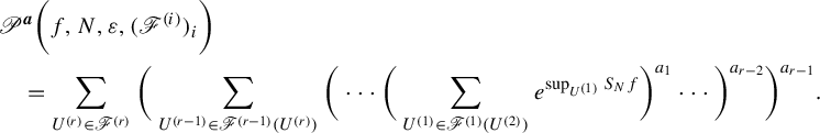 $$ \begin{align*} & \mathscr{P}^{\boldsymbol{a}}\bigg( f, N, \varepsilon, (\mathscr{F}^{(i)})_i \bigg)\\&\quad = \sum_{U^{(r)} \in \mathscr{F}^{(r)}} \bigg( \sum_{U^{(r-1)} \in \mathscr{F}^{(r-1)}(U^{(r)})} \bigg( \cdots \bigg( \sum_{U^{(1)} \in \mathscr{F}^{(1)}(U^{(2)})} e^{\sup_{U^{(1)}}S_Nf} \bigg)^{a_1} \cdots \bigg)^{a_{r-2}}\bigg)^{a_{r-1}}.\end{align*} $$
Then
 $$ \begin{align*} & P^{\boldsymbol{a}}_r(X_r, f, N, \varepsilon) \\ &\quad = \inf{ \{ \mathscr{P}^{\boldsymbol{a}}( f, N, \varepsilon, (\mathscr{F}^{(i)})_i ) | (\mathscr{F}^{(i)})_i \text{ is a chain of open } (N, \varepsilon)\text{-covers of } (X_i)_i \} }. \end{align*} $$
Just like the classic notion of pressure, we have the following property.
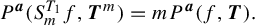
Lemma 3.3. For any natural number m,
 $$ \begin{align*} P^{\boldsymbol{a}}(S_m^{T_1}f, \boldsymbol{T}^m) = mP^{\boldsymbol{a}}(f, \boldsymbol{T}), \end{align*} $$
where
 $\boldsymbol {T}^m = ({T_i}^m)_{i=1}^r$
.
$\boldsymbol {T}^m = ({T_i}^m)_{i=1}^r$
.
Proof. Fix
 $\varepsilon> 0$
. It is obvious from the definition of
$\varepsilon> 0$
. It is obvious from the definition of
 $P^{\boldsymbol {a}}_1$
that for any
$P^{\boldsymbol {a}}_1$
that for any
 $\Omega _1 \subset X_1$
and a natural number N,
$\Omega _1 \subset X_1$
and a natural number N,
 $$ \begin{align*} P^{\boldsymbol{a}}_1(\Omega_1, S_m^{T_1}f, \boldsymbol{T}^m, N, \varepsilon) \leq P^{\boldsymbol{a}}_1(\Omega_1, f, \boldsymbol{T}, mN, \varepsilon). \end{align*} $$
Let
 $\Omega _{i+1} \subset X_{i+1}$
. By induction on i, we have
$\Omega _{i+1} \subset X_{i+1}$
. By induction on i, we have
 $$ \begin{align*} P^{\boldsymbol{a}}_i(\Omega_{i+1}, S_m^{T_1}f, \boldsymbol{T}^m, N, \varepsilon) \leq P^{\boldsymbol{a}}_i(\Omega_{i+1}, f, \boldsymbol{T}, mN, \varepsilon). \end{align*} $$
Thus,
 $$ \begin{align} P^{\boldsymbol{a}}_r(S_m^{T_1}f, \boldsymbol{T}^m, N, \varepsilon) \leq P^{\boldsymbol{a}}_r(f, \boldsymbol{T}, mN, \varepsilon). \end{align} $$
There exists
 $0 < \delta < \varepsilon $
such that for any
$0 < \delta < \varepsilon $
such that for any
 $1 \leq i \leq r$
,
$1 \leq i \leq r$
,
 $$ \begin{align*} d^{(i)}(x, y) < \delta \implies d_m^{T_i}(x, y) < \varepsilon\quad (\text{for } x, y \in X_i). \end{align*} $$
Then
 $$ \begin{align} d_N^{T_i^m}(x, y) < \delta \implies d_{mN}^{T_i}(x, y) < \varepsilon\quad (\text{for } x, y \in X_i \text{ and } 1 \leq i \leq r). \end{align} $$
Let
 $i=1$
in equation (3.2), then we have for any
$i=1$
in equation (3.2), then we have for any
 $\Omega _1 \subset X_1$
,
$\Omega _1 \subset X_1$
,
 $$ \begin{align*} P^{\boldsymbol{a}}_1(\Omega_1, f, \boldsymbol{T}, mN, \varepsilon) \leq P^{\boldsymbol{a}}_1(\Omega_1, S_m^{T_1}f, \boldsymbol{T}^m, N, \delta). \end{align*} $$
Take
 $\Omega _{i+1} \subset X_{i+1}$
. Again by induction on i and by equation (3.2), we have
$\Omega _{i+1} \subset X_{i+1}$
. Again by induction on i and by equation (3.2), we have
 $$ \begin{align*} P^{\boldsymbol{a}}_i(\Omega_{i+1}, f, \boldsymbol{T}, mN, \varepsilon) \leq P^{\boldsymbol{a}}_i(\Omega_{i+1}, S_m^{T_1}f, \boldsymbol{T}^m, N, \delta). \end{align*} $$
Hence,
 $$ \begin{align*} P^{\boldsymbol{a}}_r(f, \boldsymbol{T}, mN, \varepsilon) \leq P^{\boldsymbol{a}}_r(S_m^{T_1}f, \boldsymbol{T}^m, N, \delta).\end{align*} $$
Combining with equation (3.1), we have
 $$ \begin{align*} P^{\boldsymbol{a}}_r(S_m^{T_1}f, \boldsymbol{T}^m, N, \varepsilon) \leq P^{\boldsymbol{a}}_r(f, \boldsymbol{T}, mN, \varepsilon) \leq P^{\boldsymbol{a}}_r(S_m^{T_1}f, \boldsymbol{T}^m, N, \delta). \end{align*} $$
Therefore,
 $$ \begin{align*} P^{\boldsymbol{a}}(S^{T_1}_m f, \boldsymbol{T}^m) = mP^{\boldsymbol{a}}(f, \boldsymbol{T}).\\[-36pt] \end{align*} $$
We will later use the following standard lemma of calculus.
Lemma 3.4
-
(1) For
$0 \leq a \leq 1$
and non-negative numbers
$x, y$
,
$$ \begin{align*} (x+y)^a \leq x^a+y^a. \end{align*} $$
-
(2) Suppose that non-negative real numbers
$p_1, p_2, \ldots , p_n$
satisfy
$\sum _{i=\mathrm {1}}^n p_i = \mathrm {1}$
. Then for any real numbers
$x_1, x_2, \ldots , x_n$
, we have In particular, letting
$$ \begin{align*} \sum_{i=1}^n ( -p_i \log{p_i} +x_i p_i) \leq \log{\sum_{i=1}^n e^{x_i}}. \end{align*} $$
$x_1=x_2=\cdots =x_n=0$
gives Here,
$$ \begin{align*} \sum_{i=1}^n(-p_i \log{p_i}) \leq \log{n}. \end{align*} $$
$0 \cdot \log {0}$
is defined as
$0$
.


The proof for item (1) is elementary. See [Reference WaltersWal82, §9.3, Lemma 9.9] for item (2).
3.2. Measure theoretic entropy
In this subsection, we will introduce the classical measure-theoretic entropy (also known as Kolmogorov–Sinai entropy) and state some of the basic lemmas we need to prove Theorem 2.1. The main reference is the book of Walters [Reference WaltersWal82].
Let
 $(X, T)$
be a dynamical system and
$(X, T)$
be a dynamical system and
 $\mu \in \mathscr {M}^T(X)$
. A set
$\mu \in \mathscr {M}^T(X)$
. A set
 $\mathscr {A} = \{A_1, \ldots , A_n\}$
is called a finite partition of X with measurable elements if
$\mathscr {A} = \{A_1, \ldots , A_n\}$
is called a finite partition of X with measurable elements if
 $X = A_1 \cup \cdots \cup A_n$
, each
$X = A_1 \cup \cdots \cup A_n$
, each
 $A_i$
is a measurable set, and
$A_i$
is a measurable set, and
 $A_i \cap A_j = \varnothing $
for
$A_i \cap A_j = \varnothing $
for
 $i \ne j$
. In this paper, a partition is always finite and consists of measurable elements.
$i \ne j$
. In this paper, a partition is always finite and consists of measurable elements.
Let
 $\mathscr {A}$
and
$\mathscr {A}$
and
 $\mathscr {A}'$
be partitions of X. We define a new partition
$\mathscr {A}'$
be partitions of X. We define a new partition
 $\mathscr {A} \vee \mathscr {A}'$
by
$\mathscr {A} \vee \mathscr {A}'$
by
 $$ \begin{align*} \mathscr{A} \vee \mathscr{A}' = \{ A \cap A' | A \in \mathscr{A} \text{ and } A' \in \mathscr{A}' \}. \end{align*} $$
For a natural number N, we define a refined partition
 $\mathscr {A}_N$
of
$\mathscr {A}_N$
of
 $\mathscr {A}$
by
$\mathscr {A}$
by
 $$ \begin{align*} \mathscr{A}_N = \mathscr{A} \vee T^{-1}\mathscr{A} \vee T^{-2}\mathscr{A} \vee \cdots \vee T^{-(N-1)}\mathscr{A}, \end{align*} $$
where
 $T^{-i}\mathscr {A} = \{ T^{-i}(A) | A \in \mathscr {A}\}$
is a partition for
$T^{-i}\mathscr {A} = \{ T^{-i}(A) | A \in \mathscr {A}\}$
is a partition for
 $i \in \mathbb {N}$
.
$i \in \mathbb {N}$
.
For a partition
 $\mathscr {A}$
of X, let
$\mathscr {A}$
of X, let
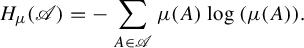 $$ \begin{align*} H_\mu(\mathscr{A}) = - \sum_{A \in \mathscr{A}} \mu(A) \log{(\mu(A))}. \end{align*} $$
We set
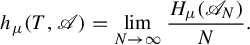 $$ \begin{align*} h_\mu(T, \mathscr{A}) = \lim_{N \to \infty} \frac{H_\mu(\mathscr{A}_N)}{N}. \end{align*} $$
This limit exists since
 $H_\mu (\mathscr {A}_N)$
is sub-additive in N. The measure theoretic entropy
$H_\mu (\mathscr {A}_N)$
is sub-additive in N. The measure theoretic entropy
 $h_\mu (T)$
is defined by
$h_\mu (T)$
is defined by
 $$ \begin{align*} h_\mu(T) = \sup \{ h_\mu(T, \mathscr{A}) | \mathscr{A} \text{ is a partition of } X \}. \end{align*} $$
Let
 $\mathscr {A}$
and
$\mathscr {A}$
and
 $\mathscr {A}'$
be partitions. Their conditional entropy is defined by
$\mathscr {A}'$
be partitions. Their conditional entropy is defined by
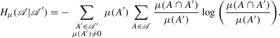 $$ \begin{align*} H_\mu(\mathscr{A} | \mathscr{A}') = - \sum_{\substack{A' \in \mathscr{A}' \\ \mu(A') \ne 0}} \mu(A') \sum_{A \in \mathscr{A}} \frac{\mu(A \cap A')}{\mu(A')} \log{\bigg( \frac{\mu(A \cap A')}{\mu(A')} \bigg)}. \end{align*} $$
Lemma 3.5
-
(1)
$H_\mu (\mathscr {A})$
is sub-additive in
$\mathscr {A}$
: that is, for partitions
$\mathscr {A}$
and
$\mathscr {A}'$
,
$$ \begin{align*} H_\mu(\mathscr{A} \vee \mathscr{A}') \leq H_\mu(\mathscr{A}) + H_\mu(\mathscr{A}'). \end{align*} $$
-
(2)
$H_\mu (\mathscr {A})$
is concave in
$\mu $
: that is, for
$\mu , \nu \in \mathscr {M}^T(X)$
and
$0 \leq t \leq 1$
,
$$ \begin{align*} H_{(1-t)\mu+t\nu}(\mathscr{A}) \geq (1-t)H_\mu(\mathscr{A}) + tH_\nu(\mathscr{A}). \end{align*} $$
-
(3) For partitions
$\mathscr {A}$
and
$\mathscr {A}'$
,
$$ \begin{align*} h_\mu(T, \mathscr{A}) \leq h_\mu(T, \mathscr{A}') + H_\mu(\mathscr{A}' | \mathscr{A}). \end{align*} $$


For the proof, confer with [Reference WaltersWal82, Theorem 4.3(viii), §4.5] for item (1), [Reference WaltersWal82, Remark, §8.1] for item (2), and [Reference WaltersWal82, Theorem 4.12, §4.5] for item (3).
3.3. Zero-dimensional principal extension
Here we will see how we can reduce the proof of
 $P^{\boldsymbol {a}}(f) \leq P^{\boldsymbol {a}}_{\mathrm {var}}(f)$
to the case where all dynamical systems are zero- dimensional.
$P^{\boldsymbol {a}}(f) \leq P^{\boldsymbol {a}}_{\mathrm {var}}(f)$
to the case where all dynamical systems are zero- dimensional.
First, we review the definitions and properties of (zero-dimensional) principal extension. The introduction here closely follows Tsukamoto’s paper [Reference TsukamotoTsu22] and the book of Downarowicz [Reference DownarowiczDow11]. Suppose
 $\pi : (Y, S) \rightarrow (X, T)$
is a factor map between dynamical systems. Let d be a metric on Y. We define the conditional topological entropy of
$\pi : (Y, S) \rightarrow (X, T)$
is a factor map between dynamical systems. Let d be a metric on Y. We define the conditional topological entropy of
 $\pi $
by
$\pi $
by
 $$ \begin{align*} h_{\mathrm{top}}(Y, S | X, T) = \lim_{\varepsilon \to 0} \bigg( \lim_{N \to \infty} \frac{\sup_{x \in X} \log{\#(\pi^{-1}(x), N, \varepsilon)}}{N} \bigg). \end{align*} $$
Here,
 $$ \begin{align*} \#(\pi^{-1}(x), N, \varepsilon) &= \min \bigg\{ n \in \mathbb{N} \bigg|\! \begin{array}{l} \text{There exists an open cover } \{U_j\}_{j=1}^n \text{ of } \pi^{-1}(x) \\ \text{with } \mathrm{diam}(U_j, d_N) < \varepsilon \text{ for all } 1 \leq j \leq n \end{array} \!\!\bigg\}. \end{align*} $$
A factor map
 $\pi : (Y, S) \rightarrow (X, T)$
between dynamical systems is said to be a principal factor map if
$\pi : (Y, S) \rightarrow (X, T)$
between dynamical systems is said to be a principal factor map if
 $$ \begin{align*} h_{\mathrm{top}}(Y, S | X, T) = 0. \end{align*} $$
Also,
 $(Y, S)$
is called a principal extension of
$(Y, S)$
is called a principal extension of
 $(X, T)$
.
$(X, T)$
.
The following theorem is from [Reference DownarowiczDow11, Corollary 6.8.9].
Theorem 3.6. Suppose
 $\pi : (Y, S) \rightarrow (X, T)$
is a principal factor map. Then
$\pi : (Y, S) \rightarrow (X, T)$
is a principal factor map. Then
 $\pi $
preserves measure-theoretic entropy, namely,
$\pi $
preserves measure-theoretic entropy, namely,
 $$ \begin{align*} h_\mu(S) = h_{\pi_*\mu}(T) \end{align*} $$
for any S-invariant probability measure
 $\mu $
on Y.
$\mu $
on Y.
More precisely, it is proved in [Reference DownarowiczDow11, Corollary 6.8.9] that
 $\pi $
is a principal factor map if and only if it preserves measure-theoretic entropy, provided that
$\pi $
is a principal factor map if and only if it preserves measure-theoretic entropy, provided that
 $h_{\mathrm {top}}(X, T) < \infty $
.
$h_{\mathrm {top}}(X, T) < \infty $
.
Suppose
 $\pi : (X_1, T_1) \rightarrow (X_2, T_2)$
and
$\pi : (X_1, T_1) \rightarrow (X_2, T_2)$
and
 $\phi : (Y, S) \rightarrow (X_2, T_2)$
are factor maps between dynamical systems. We define a fiber product
$\phi : (Y, S) \rightarrow (X_2, T_2)$
are factor maps between dynamical systems. We define a fiber product
 $(X_1 \times _{X_2}^{} Y, T_1 \times S)$
of
$(X_1 \times _{X_2}^{} Y, T_1 \times S)$
of
 $(X_1, T_1)$
and
$(X_1, T_1)$
and
 $(Y, S)$
over
$(Y, S)$
over
 $(X_2, T_2)$
by
$(X_2, T_2)$
by
 $$ \begin{align*} X_1 \times_{X_2}^{} Y = \{ (x, y) \in X_1 \times Y | \pi(x) = \phi(y) \}, \end{align*} $$
 $$ \begin{align*} T_1 \times S: X_1 \times_{X_2}^{} Y \ni (x, y) \longmapsto (T_1(x), S(y)) \in X_1 \times_{X_2}^{} Y. \end{align*} $$
We have the following commutative diagram:
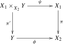
Here,
 $\pi '$
and
$\pi '$
and
 $\psi $
are restrictions of the projections onto Y and
$\psi $
are restrictions of the projections onto Y and
 $X_1$
, respectively:
$X_1$
, respectively:
 $$ \begin{align*} \pi': X_1 \times_{X_2}^{} Y \ni (x, y) \longmapsto y \in Y, \end{align*} $$
 $$ \begin{align*} \psi: X_1 \times_{X_2}^{} Y \ni (x, y) \longmapsto x \in X_1. \end{align*} $$
Since
 $\pi $
and
$\pi $
and
 $\phi $
are surjective, both
$\phi $
are surjective, both
 $\pi '$
and
$\pi '$
and
 $\psi $
are factor maps. The following lemma is proved in [Reference TsukamotoTsu22, Lemma 5.3].
$\psi $
are factor maps. The following lemma is proved in [Reference TsukamotoTsu22, Lemma 5.3].
Lemma 3.7. If
 $\phi $
is a principal extension in the diagram in equation (3.3), then
$\phi $
is a principal extension in the diagram in equation (3.3), then
 $\psi $
is also a principal extension.
$\psi $
is also a principal extension.
A dynamical system
 $(Y, S)$
is said to be zero-dimensional if there is a clopen basis of the topology of Y, where clopen means any element in the basis is both closed and open. A basic example of a zero-dimensional dynamical system is the Cantor set
$(Y, S)$
is said to be zero-dimensional if there is a clopen basis of the topology of Y, where clopen means any element in the basis is both closed and open. A basic example of a zero-dimensional dynamical system is the Cantor set
 $\{ 0, 1 \}^{\mathbb {N}}$
with the shift map.
$\{ 0, 1 \}^{\mathbb {N}}$
with the shift map.
A principal extension
 $(Y, S)$
of
$(Y, S)$
of
 $(X, T)$
is called a zero-dimensional principal extension if
$(X, T)$
is called a zero-dimensional principal extension if
 $(Y, S)$
is zero-dimensional. The following important theorem can be found in [Reference DownarowiczDow11, Theorem 7.6.1].
$(Y, S)$
is zero-dimensional. The following important theorem can be found in [Reference DownarowiczDow11, Theorem 7.6.1].
Theorem 3.8. For any dynamical system, there is a zero-dimensional principal extension.
Let
 $(Y_i, R_i)$
(
$(Y_i, R_i)$
(
 $i=1, 2, \ldots , m$
) be dynamical systems,
$i=1, 2, \ldots , m$
) be dynamical systems,
 $\pi _i: Y_i \rightarrow Y_{i+1}\, (i=1, 2, \ldots , m-1)$
factor maps, and
$\pi _i: Y_i \rightarrow Y_{i+1}\, (i=1, 2, \ldots , m-1)$
factor maps, and
 $\boldsymbol {a} = (a_1, \ldots , a_{m-1}) \in [0, 1]^{m-1}$
. Fix
$\boldsymbol {a} = (a_1, \ldots , a_{m-1}) \in [0, 1]^{m-1}$
. Fix
 $2 \leq k \leq m-1$
and take a zero-dimensional principal extension
$2 \leq k \leq m-1$
and take a zero-dimensional principal extension
 $\phi _k: (Z_k, S_k) \rightarrow (Y_k, R_k)$
. For each
$\phi _k: (Z_k, S_k) \rightarrow (Y_k, R_k)$
. For each
 $1 \leq i \leq k-1$
, let
$1 \leq i \leq k-1$
, let
 $(Y_i \times _{Y_k} Z_k, R_i \times S_k)$
be the fiber product and
$(Y_i \times _{Y_k} Z_k, R_i \times S_k)$
be the fiber product and
 $\phi _i: Y_i \times _{Y_k} Z_k \rightarrow Y_i$
be the restriction of the projection as in the earlier definition. We have
$\phi _i: Y_i \times _{Y_k} Z_k \rightarrow Y_i$
be the restriction of the projection as in the earlier definition. We have
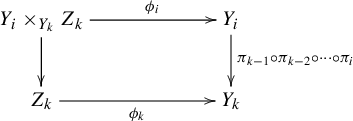
By Lemma 3.7,
 $\phi _i$
is a principal factor map. We define
$\phi _i$
is a principal factor map. We define
 $\Pi _i: Y_i \times _{Y_k} Z_k \rightarrow Y_{i+1} \times _{Y_k} Z_k$
by
$\Pi _i: Y_i \times _{Y_k} Z_k \rightarrow Y_{i+1} \times _{Y_k} Z_k$
by
 $\Pi _i(x, y) = ( \pi _i(x), y )$
for each
$\Pi _i(x, y) = ( \pi _i(x), y )$
for each
 $1 \leq i \leq k-2$
, and
$1 \leq i \leq k-2$
, and
 $\Pi _{k-1}: Y_{k-1} \times _{Y_k} Z_k \rightarrow Z_k$
as the projection. Then we have the following commutative diagram:
$\Pi _{k-1}: Y_{k-1} \times _{Y_k} Z_k \rightarrow Z_k$
as the projection. Then we have the following commutative diagram:
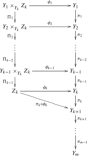
Let
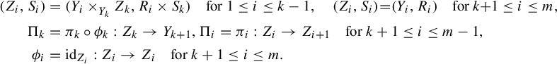 $$ \begin{align*} \begin{aligned} (Z_i, S_i) &= (Y_i \times^{}_{Y_k} Z_k, R_i \times S_k)\quad\text{for } 1 \leq i \leq k-1,\quad (Z_i, S_i)\! =\! (Y_i, R_i) \quad\text{for } k\!+\!1 \leq i \leq m, \\\Pi_k &= \pi_k \circ \phi_k: Z_k \rightarrow Y_{k+1}, \Pi_i = \pi_i: Z_i \rightarrow Z_{i+1}\quad \text{for } k+1 \leq i \leq m-1, \\ \phi_i &= \mathrm{id}_{Z_i}: Z_i \rightarrow Z_i \quad\text{for } k+1 \leq i \leq m. \end{aligned} \end{align*} $$
Lemma 3.9. In the settings above,
 $$ \begin{align*} P^{\boldsymbol{a}}_{\mathrm{var}}(f, \boldsymbol{R}, \boldsymbol{\pi}) \geq P^{\boldsymbol{a}}_{\mathrm{var}}(f \circ \phi_1, \boldsymbol{S}, \boldsymbol{\Pi}) \end{align*} $$
and
 $$ \begin{align*} P^{\boldsymbol{a}}(f, \boldsymbol{R}, \boldsymbol{\pi}) \leq P^{\boldsymbol{a}}(f \circ \phi_1, \boldsymbol{S}, \boldsymbol{\Pi}). \end{align*} $$
Here,
 $\boldsymbol {R} = (R_i)_i$
,
$\boldsymbol {R} = (R_i)_i$
,
 $\boldsymbol {\pi } = (\pi _i)_i$
,
$\boldsymbol {\pi } = (\pi _i)_i$
,
 $\boldsymbol {S} = (S_i)_i$
and
$\boldsymbol {S} = (S_i)_i$
and
 $\boldsymbol {\Pi } = (\Pi _i)_i$
.
$\boldsymbol {\Pi } = (\Pi _i)_i$
.
Proof. We remark that the following proof does not require
 $Z_k$
to be zero-dimensional. Let
$Z_k$
to be zero-dimensional. Let
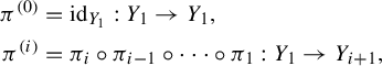 $$ \begin{align*} \pi^{(0)} &= \mathrm{id}_{Y_1}: Y_1 \to Y_1, \\ \pi^{(i)} &= \pi_i \circ \pi_{i-1} \circ \cdots \circ \pi_1: Y_1 \to Y_{i+1}, \end{align*} $$
and
 $$ \begin{align*} \Pi^{(0)} &= \mathrm{id}_{Z_1}: Z_1 \to Z_1, \\ \Pi^{(i)} &= \Pi_i \circ \Pi_{i-1} \circ \cdots \circ \Pi_1: Z_1 \to Z_{i+1}. \end{align*} $$
Let
 $\nu \in \mathscr {M}^{S_1}(Y_1)$
and
$\nu \in \mathscr {M}^{S_1}(Y_1)$
and
 $1 \leq i \leq m$
. Since all the horizontal maps in equation (3.4) are principal factor maps, we have
$1 \leq i \leq m$
. Since all the horizontal maps in equation (3.4) are principal factor maps, we have
 $$ \begin{align*} h_{{\Pi^{(i-1)}}_*\nu}(S_i) = h_{(\phi_i)_*{\Pi^{(i-1)}}_*\nu}(R_i) = h_{{\pi^{(i-1)}}_*(\phi_1)_*\nu}(R_i). \end{align*} $$
It follows that
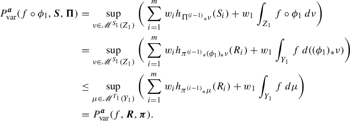 $$ \begin{align*} P^{\boldsymbol{a}}_{\mathrm{var}}(f \circ \phi_1, \boldsymbol{S}, \boldsymbol{\Pi}) &= \sup_{\nu \in \mathscr{M}^{S_1}(Z_1)} \bigg( \sum_{i=1}^{m} w_i h_{{\Pi^{(i-1)}}_*\nu} (S_i) + w_1 \int_{Z_1} f \circ \phi_1\,d\nu \bigg) \\ &= \sup_{\nu \in \mathscr{M}^{S_1}(Z_1)} \bigg( \sum_{i=1}^{m} w_i h_{{\pi^{(i-1)}}_*(\phi_1)_*\nu}(R_i) + w_1 \int_{Y_1} f\,d( (\phi_1)_*\nu ) \bigg) \\ &\leq \sup_{\mu \in \mathscr{M}^{T_1}(Y_1)} \bigg( \sum_{i=1}^{m} w_i h_{{\pi^{(i-1)}}_*\mu} (R_i) + w_1 \int_{Y_1} f\,d\mu \bigg) \\ &= P^{\boldsymbol{a}}_{\mathrm{var}}(f, \boldsymbol{R}, \boldsymbol{\pi}). \end{align*} $$
(The reversed inequality is generally true by the surjectivity of factor maps, yielding equality. However, we do not use this fact.)
Let
 $d^i$
be a metric on
$d^i$
be a metric on
 $Y_i$
for each i and
$Y_i$
for each i and
 $\widetilde {d^k}$
a metric on
$\widetilde {d^k}$
a metric on
 $Z_k$
. We define a metric
$Z_k$
. We define a metric
 $\widetilde {d^i}$
on
$\widetilde {d^i}$
on
 $(Z_i, S_i)$
for
$(Z_i, S_i)$
for
 $1 \leq i \leq k-1$
by
$1 \leq i \leq k-1$
by
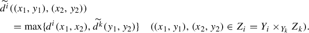 $$ \begin{align*} &\widetilde{d^i}( (x_1, y_1), (x_2, y_2) )\\ &\quad= \max\{ d^i(x_1, x_2), \widetilde{d^k}(y_1, y_2) \}\quad ((x_1, y_1), (x_2, y_2) \in Z_i = Y_i \times_{Y_k} Z_k). \end{align*} $$
Set
 $\widetilde {d^i} = d^i$
for
$\widetilde {d^i} = d^i$
for
 $k+1 \leq i \leq m$
. Take an arbitrary positive number
$k+1 \leq i \leq m$
. Take an arbitrary positive number
 $\varepsilon $
. There exists
$\varepsilon $
. There exists
 $0 < \delta < \varepsilon $
such that for every
$0 < \delta < \varepsilon $
such that for every
 $1 \leq i \leq m$
,
$1 \leq i \leq m$
,
 $$ \begin{align} \widetilde{d^i}(x, y) < \delta \implies d^i( \phi_i(x), \phi_i(y) ) < \varepsilon \quad (x, y \in Z_i). \end{align} $$
Let N be a natural number. We claim that
 $$ \begin{align*} P^{\boldsymbol{a}}_r(f, \boldsymbol{R}, \boldsymbol{\pi}, N, \varepsilon) \leq P^{\boldsymbol{a}}_r(f \circ \phi_1, \boldsymbol{S}, \boldsymbol{\Pi}, N, \delta). \end{align*} $$
Take
 $M> 0$
with
$M> 0$
with
 $$ \begin{align*} P^{\boldsymbol{a}}_r(f \circ \phi_1, \boldsymbol{S}, \boldsymbol{\Pi}, N, \delta) < M.\end{align*} $$
Then there exists a chain of open (N,
 $\delta $
)-covers
$\delta $
)-covers
 $(\mathscr {F}^{(i)})_i$
of
$(\mathscr {F}^{(i)})_i$
of
 $(Z_i)_i$
(see Definition 3.1 and Remark 3.2) with
$(Z_i)_i$
(see Definition 3.1 and Remark 3.2) with
 $$ \begin{align*} \mathscr{P}^{\boldsymbol{a}}(f \circ \phi_1, \boldsymbol{S}, \boldsymbol{\Pi}, N, \delta, (\mathscr{F}^{(i)})_i ) < M. \end{align*} $$
We can find a compact set
 $C_U \subset U$
for each
$C_U \subset U$
for each
 $U \in \mathscr {F}^{(m)}$
such that
$U \in \mathscr {F}^{(m)}$
such that
 $\bigcup _{U \in \mathscr {F}^{(m)}} C_U = Z_m$
. Let
$\bigcup _{U \in \mathscr {F}^{(m)}} C_U = Z_m$
. Let
 $\mathscr {K}^{(m)} := \{ C_U | U \in \mathscr {F}^{(m)} \}$
. Since
$\mathscr {K}^{(m)} := \{ C_U | U \in \mathscr {F}^{(m)} \}$
. Since
 $\Pi _{m-1}^{-1}(C_U) \subset \Pi _{m-1}^{-1}(U)$
is compact for each
$\Pi _{m-1}^{-1}(C_U) \subset \Pi _{m-1}^{-1}(U)$
is compact for each
 $U \in \mathscr {F}^{(m)}$
, we can find a compact set
$U \in \mathscr {F}^{(m)}$
, we can find a compact set
 $E_V \subset V$
for each
$E_V \subset V$
for each
 $V \in \mathscr {F}^{(m-1)}(U)$
such that
$V \in \mathscr {F}^{(m-1)}(U)$
such that
 $\Pi _{m-1}^{-1}(C_U) \subset \bigcup _{V \in \mathscr {F}^{(k)}(U)} E_V$
. Let
$\Pi _{m-1}^{-1}(C_U) \subset \bigcup _{V \in \mathscr {F}^{(k)}(U)} E_V$
. Let
 $\mathscr {K}^{(m-1)}(C_U) := \{ E_V | V \in \mathscr {F}^{(m-1)}(U) \}$
and
$\mathscr {K}^{(m-1)}(C_U) := \{ E_V | V \in \mathscr {F}^{(m-1)}(U) \}$
and
 $\mathscr {K}^{(m-1)} := \bigcup _{C \in \mathscr {K}^{(m)}} \mathscr {K}^{(m-1)}(C)$
. We continue likewise and obtain a chain of compact (N,
$\mathscr {K}^{(m-1)} := \bigcup _{C \in \mathscr {K}^{(m)}} \mathscr {K}^{(m-1)}(C)$
. We continue likewise and obtain a chain of compact (N,
 $\delta $
)-covers
$\delta $
)-covers
 $(\mathscr {K}^{(i)})_i$
of
$(\mathscr {K}^{(i)})_i$
of
 $(Z_i)_i$
with
$(Z_i)_i$
with
 $$ \begin{align*} \mathscr{P}^{\boldsymbol{a}}(f \circ \phi_1, \boldsymbol{S}, \boldsymbol{\Pi}, N, \delta, (\mathscr{K}^{(i)})_i) \leq \mathscr{P}^{\boldsymbol{a}}(f \circ \phi_1, \boldsymbol{S}, \boldsymbol{\Pi}, N, \delta, (\mathscr{F}^{(i)})_i ) < M. \end{align*} $$
Let
 $\phi _i(\mathscr {K}^{(i)}) = \{ \phi _i(C) | C \in \mathscr {K}^{(i)} \}$
for each i. Note that for any
$\phi _i(\mathscr {K}^{(i)}) = \{ \phi _i(C) | C \in \mathscr {K}^{(i)} \}$
for each i. Note that for any
 $\Omega \subset Z_i$
,
$\Omega \subset Z_i$
,
 $$ \begin{align*} \pi_{i-1}^{-1} ( \phi_{i} ( \Omega ) ) = \phi_{i-1} ( \Pi_{i-1}^{-1} ( \Omega ) ). \end{align*} $$
This and equation (3.5) assure that
 $(\phi _i(\mathscr {K}^{(i)}))_i$
is a chain of compact (N,
$(\phi _i(\mathscr {K}^{(i)}))_i$
is a chain of compact (N,
 $\varepsilon $
)-covers of
$\varepsilon $
)-covers of
 $(Y_i)_i$
. We have
$(Y_i)_i$
. We have
 $$ \begin{align*} \mathscr{P}^{\boldsymbol{a}}( f, \boldsymbol{R}, \boldsymbol{\pi}, N, \varepsilon, (\phi_i(\mathscr{K}^{(i)}))_i) &=\mathscr{P}^{\boldsymbol{a}} ( f \circ \phi_1, \boldsymbol{S}, \boldsymbol{\Pi}, N, \delta, (\mathscr{K}^{(i)})_i) < M. \end{align*} $$
Since f is continuous and each
 $\phi _i(\mathscr {K}^{(i)})$
is a closed cover, we can slightly enlarge each set in
$\phi _i(\mathscr {K}^{(i)})$
is a closed cover, we can slightly enlarge each set in
 $\phi _i(\mathscr {K}^{(i)})$
and create a chain of open (N,
$\phi _i(\mathscr {K}^{(i)})$
and create a chain of open (N,
 $\varepsilon $
)-covers
$\varepsilon $
)-covers
 $(\mathscr {O}^{(i)})_i$
of
$(\mathscr {O}^{(i)})_i$
of
 $(Y_i)_i$
satisfying
$(Y_i)_i$
satisfying
 $$ \begin{align*} \mathscr{P}^{\boldsymbol{a}}( f, \boldsymbol{R}, \boldsymbol{\pi}, N, \varepsilon, (\mathscr{O}^{(i)})_i ) < M. \end{align*} $$
Therefore,
 $$ \begin{align*} P^{\boldsymbol{a}}_r(f, \boldsymbol{R}, \boldsymbol{\pi}, N, \varepsilon) \leq \mathscr{P}^{\boldsymbol{a}}( f, \boldsymbol{R}, \boldsymbol{\pi}, N, \varepsilon, (\mathscr{O}^{(i)})_i) < M. \end{align*} $$
Since
 $M> P^{\boldsymbol {a}}_r(f \circ \phi _1, \boldsymbol {S}, \boldsymbol {\Pi }, N, \delta )$
was chosen arbitrarily, we have
$M> P^{\boldsymbol {a}}_r(f \circ \phi _1, \boldsymbol {S}, \boldsymbol {\Pi }, N, \delta )$
was chosen arbitrarily, we have
 $$ \begin{align*} P^{\boldsymbol{a}}_r(f, \boldsymbol{R}, \boldsymbol{\pi}, N, \varepsilon) \leq P^{\boldsymbol{a}}_r(f \circ \phi_1, \boldsymbol{S}, \boldsymbol{\Pi}, N, \delta). \end{align*} $$
This implies
 $$ \begin{align*} P^{\boldsymbol{a}}(f, \boldsymbol{R}, \boldsymbol{\pi}) \leq P^{\boldsymbol{a}}(f \circ \phi_1, \boldsymbol{S}, \boldsymbol{\Pi}).\\[-35pt] \end{align*} $$
The following proposition reduces the proof of
 $P^{\boldsymbol {a}}(f) \leq P^{\boldsymbol {a}}_{\mathrm {var}}(f)$
in the next section to the case where all dynamical systems are zero-dimensional.
$P^{\boldsymbol {a}}(f) \leq P^{\boldsymbol {a}}_{\mathrm {var}}(f)$
in the next section to the case where all dynamical systems are zero-dimensional.
Proposition 3.10. For all dynamical systems
 $(X_i, T_i)$
(
$(X_i, T_i)$
(
 $i=1, 2, \ldots , r$
) and factor maps
$i=1, 2, \ldots , r$
) and factor maps
 $\pi _i: X_i \rightarrow X_{i+1}\ (i=1, 2, \ldots , r-1)$
, there are zero-dimensional dynamical systems
$\pi _i: X_i \rightarrow X_{i+1}\ (i=1, 2, \ldots , r-1)$
, there are zero-dimensional dynamical systems
 $(Z_i, S_i)\ (i=1, 2, \ldots , r)$
and factor maps
$(Z_i, S_i)\ (i=1, 2, \ldots , r)$
and factor maps
 $\Pi _i: Z_i \rightarrow Z_{i+1}\ (i=1, 2, \ldots , r-1)$
with the following property; for every continuous function
$\Pi _i: Z_i \rightarrow Z_{i+1}\ (i=1, 2, \ldots , r-1)$
with the following property; for every continuous function
 $f: X_1 \rightarrow \mathbb {R}$
, there exists a continuous function
$f: X_1 \rightarrow \mathbb {R}$
, there exists a continuous function
 $g: Z_1 \rightarrow \mathbb {R}$
with
$g: Z_1 \rightarrow \mathbb {R}$
with
 $$ \begin{align*} P^{\boldsymbol{a}}_{\mathrm{var}}(f, \boldsymbol{T}, \boldsymbol{\pi}) \geq P^{\boldsymbol{a}}_{\mathrm{var}}(g, \boldsymbol{S}, \boldsymbol{\Pi}) \end{align*} $$
and
 $$ \begin{align*} P^{\boldsymbol{a}}(f, \boldsymbol{T}, \boldsymbol{\pi}) \leq P^{\boldsymbol{a}}(g, \boldsymbol{S}, \boldsymbol{\Pi}). \end{align*} $$
Proof. We will first construct zero-dimensional dynamical systems
 $(Z_i, S_i)$
(
$(Z_i, S_i)$
(
 $i=1, 2, \ldots , r$
) and factor maps
$i=1, 2, \ldots , r$
) and factor maps
 $\Pi _i: Z_i \rightarrow Z_{i+1}\ (i=1, 2, \ldots , r-1)$
alongside the following commutative diagram of dynamical systems and factor maps:
$\Pi _i: Z_i \rightarrow Z_{i+1}\ (i=1, 2, \ldots , r-1)$
alongside the following commutative diagram of dynamical systems and factor maps:
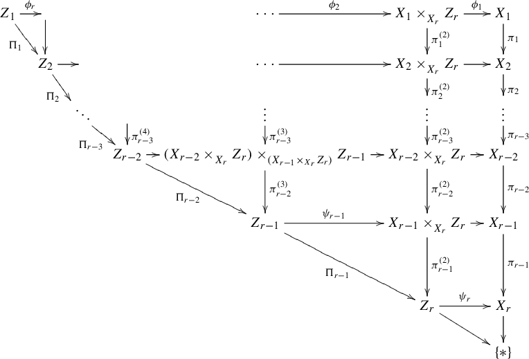
where all the horizontal maps are principal factor maps.
By Theorem 3.8, there is a zero-dimensional principal extension
 $\psi _r: (Z_r, S_r) \rightarrow (X_r, T_r)$
. The set
$\psi _r: (Z_r, S_r) \rightarrow (X_r, T_r)$
. The set
 $\{*\}$
is the trivial dynamical system, and the maps
$\{*\}$
is the trivial dynamical system, and the maps
 $X_r \rightarrow \{*\}$
and
$X_r \rightarrow \{*\}$
and
 $Z_r \rightarrow \{*\}$
send every element to
$Z_r \rightarrow \{*\}$
send every element to
 $*$
. For each
$*$
. For each
 $1 \leq i \leq r-1$
, the map
$1 \leq i \leq r-1$
, the map
 $X_i \times _{X_r}^{} Z_r \rightarrow X_i$
in the following diagram is a principal factor map by Lemma 3.7:
$X_i \times _{X_r}^{} Z_r \rightarrow X_i$
in the following diagram is a principal factor map by Lemma 3.7:
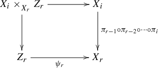
For
 $1 \leq i \leq r-2$
, define
$1 \leq i \leq r-2$
, define
 $\pi _i^{(2)}: X_i \times _{X_r}^{} Z_r \rightarrow X_{i+1} \times _{X_r}^{} Z_r$
by
$\pi _i^{(2)}: X_i \times _{X_r}^{} Z_r \rightarrow X_{i+1} \times _{X_r}^{} Z_r$
by
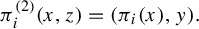 $$ \begin{align*} \pi_i^{(2)}(x, z) = (\pi_i(x), y). \end{align*} $$
Then every horizontal map in the right two rows of diagram (3.6) is a principal factor map. Next, take a zero-dimensional principal extension
 $\psi _{r-1}: (Z_{r-1}, S_{r-1}) \rightarrow (X_{r-1} \times _{X_r}^{} Z_r, T_{r-1} \times S_r)$
and let
$\psi _{r-1}: (Z_{r-1}, S_{r-1}) \rightarrow (X_{r-1} \times _{X_r}^{} Z_r, T_{r-1} \times S_r)$
and let
 $\Pi _{r-1} = \pi _{r-1}^{(2)} \circ \psi _{r-1}$
. The rest of diagram (3.6) is constructed similarly, and by Lemma 3.7, each horizontal map is a principal factor map.
$\Pi _{r-1} = \pi _{r-1}^{(2)} \circ \psi _{r-1}$
. The rest of diagram (3.6) is constructed similarly, and by Lemma 3.7, each horizontal map is a principal factor map.
Let
 $f: X_1 \rightarrow \mathbb {R}$
be a continuous map. Applying Lemma 3.9 to the right two rows of diagram (3.6), we get
$f: X_1 \rightarrow \mathbb {R}$
be a continuous map. Applying Lemma 3.9 to the right two rows of diagram (3.6), we get
 $$ \begin{align*} P^{\boldsymbol{a}}_{\mathrm{var}}(f, \boldsymbol{T}, \boldsymbol{\pi}) \geq P^{\boldsymbol{a}}_{\mathrm{var}}(f \circ \phi_1, \boldsymbol{S^{(2)}}, \boldsymbol{\Pi^{(2)}}) \end{align*} $$
and
 $$ \begin{align*} P^{\boldsymbol{a}}(f, \boldsymbol{T}, \boldsymbol{\pi}) \leq P^{\boldsymbol{a}}(f \circ \phi_1, \boldsymbol{S^{(2)}}, \boldsymbol{\Pi^{(2)}}) \end{align*} $$
for
 $\boldsymbol {\Pi ^{(2)}} = (\pi ^{(2)}_i)_i$
and
$\boldsymbol {\Pi ^{(2)}} = (\pi ^{(2)}_i)_i$
and
 $\boldsymbol {S^{(2)}} = (T_i \times S_r)_i$
. Again by Lemma 3.9,
$\boldsymbol {S^{(2)}} = (T_i \times S_r)_i$
. Again by Lemma 3.9,
 $$ \begin{align*} P^{\boldsymbol{a}}_{\mathrm{var}}(f \circ \phi_1, \boldsymbol{S^{(2)}}, \boldsymbol{\Pi^{(2)}}) \geq P^{\boldsymbol{a}}_{\mathrm{var}}(f \circ \phi_1 \circ \phi_2, \boldsymbol{S^{(3)}}, \boldsymbol{\Pi^{(3)}}) \end{align*} $$
and
 $$ \begin{align*} P^{\boldsymbol{a}}(f \circ \phi_1, \boldsymbol{S^{(2)}}, \boldsymbol{\Pi^{(2)}}) \leq P^{\boldsymbol{a}}(f \circ \phi_1 \circ \phi_2, \boldsymbol{S^{(3)}}, \boldsymbol{\Pi^{(3)}}) \end{align*} $$
where
 $\boldsymbol {\Pi ^{(3)}} = ( (\pi ^{(3)}_i)_{i=1}^{r-2}, \Pi _{r-1})$
, and
$\boldsymbol {\Pi ^{(3)}} = ( (\pi ^{(3)}_i)_{i=1}^{r-2}, \Pi _{r-1})$
, and
 $\boldsymbol {S^{(3)}}$
is the collection of maps associated with
$\boldsymbol {S^{(3)}}$
is the collection of maps associated with
 $Z_r$
and the third row from the right of diagram (3.6). We continue inductively and obtain the desired inequalities, where g is taken as
$Z_r$
and the third row from the right of diagram (3.6). We continue inductively and obtain the desired inequalities, where g is taken as
 $f \circ \phi _1 \circ \phi _2 \circ \cdots \circ \phi _r$
.
$f \circ \phi _1 \circ \phi _2 \circ \cdots \circ \phi _r$
.
4. Proof of
$P^{\boldsymbol {a}}(f) \leq P^{\boldsymbol {a}}_{\mathrm {var}}(f)$

Let
 $\boldsymbol {a} = (a_1, \ldots , a_{r-1}) \in [0, 1]^{r-1}$
. Recall that we defined
$\boldsymbol {a} = (a_1, \ldots , a_{r-1}) \in [0, 1]^{r-1}$
. Recall that we defined
 $(w_1, \ldots , w_r)$
by
$(w_1, \ldots , w_r)$
by
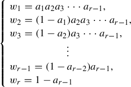 $$ \begin{align*} \left\{\! \begin{array}{l} w_1 = a_1 a_2 a_3 \cdots a_{r-1},\\w_2 = (1-a_1) a_2 a_3 \cdots a_{r-1}, \\w_3 = (1-a_2) a_3 \cdots a_{r-1}, \\\kern55pt \vdots \\ w_{r-1} = (1-a_{r-2}) a_{r-1}, \\ w_r = 1- a_{r-1} \end{array} \right. \end{align*} $$
and
 $P^{\boldsymbol {a}}_{\mathrm {var}}(f)$
by
$P^{\boldsymbol {a}}_{\mathrm {var}}(f)$
by
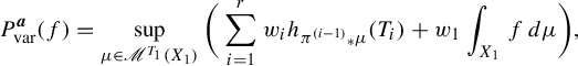 $$ \begin{align*} P^{\boldsymbol{a}}_{\mathrm{var}}(f) = \sup_{\mu \in \mathscr{M}^{T_1}(X_1)} \bigg( \sum_{i=1}^r w_i h_{{\pi^{(i-1)}}_*\mu} (T_i) + w_1 \int_{X_1} f\,d\mu \bigg), \end{align*} $$
where
 $$ \begin{align*} \pi^{(0)} &= \mathrm{id}_{X_1}: X_1 \to X_1, \\ \pi^{(i)} &= \pi_i \circ \pi_{i-1} \circ \cdots \circ \pi_1: X_1 \to X_{i+1}. \end{align*} $$
The following theorem suffices by Proposition 3.10 in proving
 $P^{\boldsymbol {a}}(f) \leq P^{\boldsymbol {a}}_{\mathrm {var}}(f)$
for arbitrary dynamical systems.
$P^{\boldsymbol {a}}(f) \leq P^{\boldsymbol {a}}_{\mathrm {var}}(f)$
for arbitrary dynamical systems.
Theorem 4.1. Suppose
 $(X_i, T_i)$
(
$(X_i, T_i)$
(
 $i=1, 2, \ldots , r$
) are zero-dimensional dynamical systems and
$i=1, 2, \ldots , r$
) are zero-dimensional dynamical systems and
 $\pi _i: X_i \rightarrow X_{i+1}\ (i=1, 2, \ldots , r-1)$
are factor maps. Then we have
$\pi _i: X_i \rightarrow X_{i+1}\ (i=1, 2, \ldots , r-1)$
are factor maps. Then we have
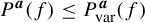 $$ \begin{align*} P^{\boldsymbol{a}}(f) \leq P^{\boldsymbol{a}}_{\mathrm{var}}(f) \end{align*} $$
for any continuous function
 $f: X_1 \rightarrow \mathbb {R}$
.
$f: X_1 \rightarrow \mathbb {R}$
.
Proof. Let
 $d^{(i)}$
be a metric on
$d^{(i)}$
be a metric on
 $X_i$
for each
$X_i$
for each
 $i=1, 2, \ldots , r$
. Take a positive number
$i=1, 2, \ldots , r$
. Take a positive number
 $\varepsilon $
and a natural number N. First, we will backward inductively define a finite clopen partition
$\varepsilon $
and a natural number N. First, we will backward inductively define a finite clopen partition
 $\mathscr {A}^{(i)}$
of
$\mathscr {A}^{(i)}$
of
 $X_i$
for each i. Since
$X_i$
for each i. Since
 $X_r$
is zero-dimensional, we can take a sufficiently fine finite clopen partition
$X_r$
is zero-dimensional, we can take a sufficiently fine finite clopen partition
 $\mathscr {A}^{(r)}$
of
$\mathscr {A}^{(r)}$
of
 $X_r $
. That is, each
$X_r $
. That is, each
 $A \in \mathscr {A}^{(r)}$
is both open and closed, and
$A \in \mathscr {A}^{(r)}$
is both open and closed, and
 $\mathrm {diam}(A, d^{(r)}_N) < \varepsilon $
. Suppose
$\mathrm {diam}(A, d^{(r)}_N) < \varepsilon $
. Suppose
 $\mathscr {A}^{(i+1)}$
is defined. For each
$\mathscr {A}^{(i+1)}$
is defined. For each
 $A \in \mathscr {A}^{(i+1)}$
, take a clopen partition
$A \in \mathscr {A}^{(i+1)}$
, take a clopen partition
 $\mathscr {B}(A)$
of
$\mathscr {B}(A)$
of
 $\pi _{i}^{-1} (A) \subset X_{i}$
such that any
$\pi _{i}^{-1} (A) \subset X_{i}$
such that any
 $B \in \mathscr {B}(A)$
satisfies
$B \in \mathscr {B}(A)$
satisfies
 $\mathrm {diam}(B, d^{(i)}_N) < \varepsilon $
. We let
$\mathrm {diam}(B, d^{(i)}_N) < \varepsilon $
. We let
 $\mathscr {A}^{(i)} = \bigcup _{A \in \mathscr {A}^{(i+1)}} \mathscr {B}(A)$
. Then
$\mathscr {A}^{(i)} = \bigcup _{A \in \mathscr {A}^{(i+1)}} \mathscr {B}(A)$
. Then
 $\mathscr {A}^{(i)}$
is a finite clopen partition of
$\mathscr {A}^{(i)}$
is a finite clopen partition of
 $X_i$
. We define
$X_i$
. We define
 $$ \begin{align*} \mathscr{A}^{(i)}_N = \mathscr{A}^{(i)} \vee T_i^{-1}\mathscr{A}^{(i)} \vee T_i^{-2}\mathscr{A}^{(i)} \vee \cdots \vee T_i^{-(N-1)}\mathscr{A}^{(i)}. \end{align*} $$
We employ the following notation. For
 $i<j$
and
$i<j$
and
 $A \in \mathscr {A}^{(j)}_N$
, let
$A \in \mathscr {A}^{(j)}_N$
, let
 $\mathscr {A}^{(i)}_N(A)$
be the set of ‘children’ of A:
$\mathscr {A}^{(i)}_N(A)$
be the set of ‘children’ of A:
 $$ \begin{align*} \mathscr{A}^{(i)}_N(A) = \{B \in \mathscr{A}^{(i)}_N | \pi_{j-1} \circ \pi_{j-2} \circ \cdots \circ \pi_i(B) \subset A \}. \end{align*} $$
Also, for
 $B \in \mathscr {A}^{(i)}_N$
and
$B \in \mathscr {A}^{(i)}_N$
and
 $i<j$
, we denote by
$i<j$
, we denote by
 $\widetilde {\pi }_j B$
the unique ‘parent’ of B in
$\widetilde {\pi }_j B$
the unique ‘parent’ of B in
 $\mathscr {A}^{(j)}_N$
:
$\mathscr {A}^{(j)}_N$
:
 $$ \begin{align*} \widetilde{\pi}_j B = A \in \mathscr{A}^{(j)}_N\quad\text{such that } \pi_{j-1} \circ \pi_{j-2} \circ \cdots \circ \pi_{i}(B) \subset A. \end{align*} $$
We will evaluate
 $P^{\boldsymbol {a}}(f, N, \varepsilon )$
from above using
$P^{\boldsymbol {a}}(f, N, \varepsilon )$
from above using
 $\{ \mathscr {A}^{(i)} \}$
. Let
$\{ \mathscr {A}^{(i)} \}$
. Let
 $A \in \mathscr {A}^{(2)}_N$
, and start by setting
$A \in \mathscr {A}^{(2)}_N$
, and start by setting
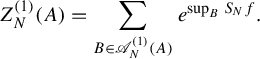 $$ \begin{align*} Z^{(1)}_N (A) = \sum_{B \in \mathscr{A}^{(1)}_N(A)} e^{\sup_B S_N f}. \end{align*} $$
Let
 $A \in \mathscr {A}^{(i+1)}_N$
. If
$A \in \mathscr {A}^{(i+1)}_N$
. If
 $Z^{(i-1)}_N$
is already defined, set
$Z^{(i-1)}_N$
is already defined, set
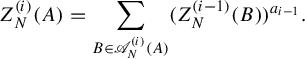 $$ \begin{align*} Z^{(i)}_N (A) = \sum_{B \in \mathscr{A}^{(i)}_N(A)} ( Z^{(i-1)}_N (B))^{a_{i-1}}. \end{align*} $$
We then define
 $Z_N$
by
$Z_N$
by
 $$ \begin{align*} Z_N = \sum_{A \in \mathscr{A}^{(r)}_N} ( Z^{(r-1)}_N (A) )^{a_{r-1}}. \end{align*} $$
It is straightforward from the construction that
 $$ \begin{align*} P^{\boldsymbol{a}}_r(X_r, f, N, \varepsilon) \leq Z_N. \end{align*} $$
Therefore, we only need to prove that there is a
 $T_1$
-invariant probability measure
$T_1$
-invariant probability measure
 $\mu $
on
$\mu $
on
 $X_1$
such that
$X_1$
such that
 $$ \begin{align*} \sum_{i=1}^r w_i h_{{\pi^{(i-1)}}_* \mu} (T_i, \mathscr{A}^{(i)}) + w_1 \int_{X_1} f\,d\mu \geq \lim_{N \to \infty} \frac{\log Z_N}{N}. \end{align*} $$
Since each
 $A \in \mathscr {A}^{(1)}_N$
is closed, we can choose a point
$A \in \mathscr {A}^{(1)}_N$
is closed, we can choose a point
 $x_A \in A$
so that
$x_A \in A$
so that
 $$ \begin{align*} S_N f(x_A) = \sup_A S_N f. \end{align*} $$
We define a probability measure
 $\sigma ^{}_N$
on
$\sigma ^{}_N$
on
 $X_1$
by
$X_1$
by
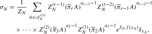 $$ \begin{align*} \sigma_N^{} &= \frac{1}{Z_N} \sum_{A \in \mathscr{A}^{(1)}_N} {Z_N^{(r-1)}(\widetilde{\pi}_{r}A)}^{a_{r-1}-1}{Z_N^{(r-2)}(\widetilde{\pi}_{r-1}A)}^{a_{r-2}-1} \\ &\quad \times \cdots \times {Z_N^{(2)}(\widetilde{\pi}_3 A)}^{a_{2}-1}{Z_N^{(1)}(\widetilde{\pi}_2 A)}^{a_{1}-1}e^{S_N f(x_A)} \delta_{x_A}, \end{align*} $$
where
 $\delta _{x^{}_A}$
is the Dirac measure at
$\delta _{x^{}_A}$
is the Dirac measure at
 $x_A$
. This is indeed a probability measure on
$x_A$
. This is indeed a probability measure on
 $X_1$
since
$X_1$
since
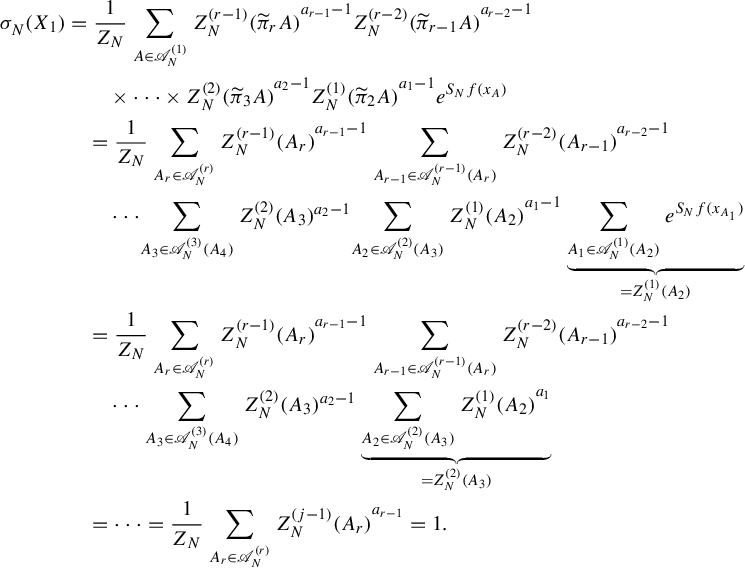 $$ \begin{align*} \sigma_N^{}(X_1) &= \frac{1}{Z_N} \sum_{A \in \mathscr{A}^{(1)}_N} {Z_N^{(r-1)}(\widetilde{\pi}_{r}A)}^{a_{r-1}-1}{Z_N^{(r-2)}(\widetilde{\pi}_{r-1}A)}^{a_{r-2}-1} \\ &\qquad \times \cdots \times {Z_N^{(2)}(\widetilde{\pi}_3 A)}^{a_{2}-1}{Z_N^{(1)}(\widetilde{\pi}_2 A)}^{a_{1}-1}e^{S_N f(x_A)} \\ &\quad=\frac{1}{Z_N} \sum_{A_r \in \mathscr{A}^{(r)}_N} {Z_N^{(r-1)}(A_r)}^{a_{r-1}-1} \sum_{A_{r-1} \in \mathscr{A}^{(r-1)}_N(A_r)} {Z_N^{(r-2)}(A_{r-1})}^{a_{r-2}-1} \\ &\qquad \cdots \!\sum_{A_3 \in \mathscr{A}^{(3)}_N(A_4)} Z_N^{(2)}(A_3)^{a_2-1}\! \sum_{A_2 \in \mathscr{A}^{(2)}_N(A_3)} {Z_N^{(1)}(A_2)}^{a_{1}-1} \underbrace{\sum_{A_1 \in \mathscr{A}^{(1)}_N(A_2)} e^{S_N f(x_{A_1})}}_{= Z_N^{(1)}(A_2)}\\ &\quad = \frac{1}{Z_N} \sum_{A_r \in \mathscr{A}^{(r)}_N} {Z_N^{(r-1)}(A_r)}^{a_{r-1}-1} \sum_{A_{r-1} \in \mathscr{A}^{(r-1)}_N(A_r)} {Z_N^{(r-2)}(A_{r-1})}^{a_{r-2}-1} \\ &\qquad \cdots \sum_{A_3 \in \mathscr{A}^{(3)}_N(A_4)} Z_N^{(2)}(A_3)^{a_2-1} \underbrace{\sum_{A_2 \in \mathscr{A}^{(2)}_N(A_3)} {Z_N^{(1)}(A_2)}^{a_{1}}}_{= Z_N^{(2)}(A_3)}\\ &\quad = \cdots = \frac{1}{Z_N} \sum_{A_r \in \mathscr{A}^{(r)}_N} {Z_N^{(j-1)}(A_r)}^{a_{r-1}} = 1. \end{align*} $$
Although
 $\sigma _N^{}$
is not generally
$\sigma _N^{}$
is not generally
 $T_1$
-invariant, the following well-known trick allows us to create a
$T_1$
-invariant, the following well-known trick allows us to create a
 $T_1$
-invariant measure
$T_1$
-invariant measure
 $\mu $
. We begin by setting
$\mu $
. We begin by setting
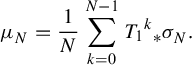 $$ \begin{align*} \mu_N^{} = \frac{1}{N} \sum_{k=0}^{N-1} {{T_1}^k}_* \sigma_N^{}. \end{align*} $$
Since
 $X_1$
is compact, we can take a sub-sequence of
$X_1$
is compact, we can take a sub-sequence of
 $(\mu _N^{})_N$
so that it weakly converges to a probability measure
$(\mu _N^{})_N$
so that it weakly converges to a probability measure
 $\mu $
on
$\mu $
on
 $X_1$
. Then
$X_1$
. Then
 $\mu $
is
$\mu $
is
 $T_1$
-invariant by the definition of
$T_1$
-invariant by the definition of
 $\mu _N$
. We will show that this
$\mu _N$
. We will show that this
 $\mu $
satisfies
$\mu $
satisfies
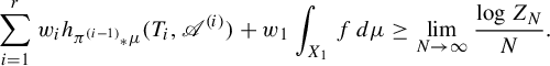 $$ \begin{align*} \sum_{i=1}^r w_i h_{{\pi^{(i-1)}}_* \mu} (T_i, \mathscr{A}^{(i)}) + w_1 \int_{X_1} f\,d\mu \geq \lim_{N \to \infty} \frac{\log Z_N}{N}. \end{align*} $$
We first prove
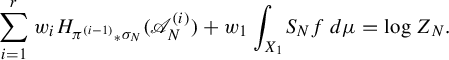 $$ \begin{align*} \sum_{i=1}^r w_i H_{{\pi^{(i-1)}}_* \sigma_N} (\mathscr{A}^{(i)}_N) + w_1 \int_{X_1} \! S_N f\,d\mu = \log Z_N. \end{align*} $$
To simplify the notation, let
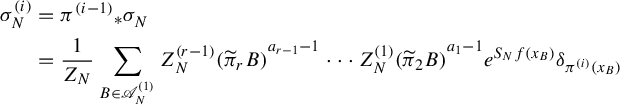 $$ \begin{align*} \sigma_N^{(i)} &= {\pi^{(i-1)}}_* \sigma_N^{} \\ &= \frac{1}{Z_N} \sum_{B \in \mathscr{A}^{(1)}_N}{Z_N^{(r-1)}(\widetilde{\pi}_r B)}^{a_{r-1}-1} \cdots {Z_N^{(1)}(\widetilde{\pi}_2 B)}^{a_{1}-1}e^{S_N f(x_B)} \delta_{\pi^{(i)} (x_B)} \end{align*} $$
and
 $$ \begin{align*} W_N^{(j)} = \sum_{A \in \mathscr{A}^{(j+1)}_N} {Z_N^{(r-1)}(\widetilde{\pi}_r A)}^{a_{r-1}-1} \cdots {Z_N^{(j+1)}(\widetilde{\pi}_{j+2} A)}^{a_{j+1}-1}{Z_N^{(j)}(A)}^{a_{j}} \log{( Z_N^{(j)}(A) )}. \end{align*} $$
Claim 4.2. We have the following equations:
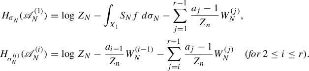 $$ \begin{align*} H_{\sigma_N^{}}(\mathscr{A}^{(1)}_N) &= \log{Z_N} - \int_{X_1} \! S_N f\,d\sigma_N^{} -\sum_{j=1}^{r-1} \frac{a_{j}-1}{Z_n} W_N^{(j)}, \\ H_{\sigma_N^{(i)}}(\mathscr{A}^{(i)}_N) &= \log{Z_N} - \frac{a_{i-1}}{Z_n} W_N^{(i-1)} - \sum_{j=i}^{r-1} \frac{a_{j}-1}{Z_n} W_N^{(j)}\quad (\textit{for } 2 \leq i \leq r ). \end{align*} $$
Here,
 $\sum _{j=r}^{r-1}\ ((a_{j}-1)/Z_n) W_N^{(j)}$
is defined to be
$\sum _{j=r}^{r-1}\ ((a_{j}-1)/Z_n) W_N^{(j)}$
is defined to be
 $0$
.
$0$
.
Proof. Let
 $A \in \mathscr {A}^{(1)}_N$
. We have
$A \in \mathscr {A}^{(1)}_N$
. We have
 $$ \begin{align*} \sigma_N^{}(A) = \frac{1}{Z_N} {Z_N^{(r-1)}(\widetilde{\pi}_r A)}^{a_{r-1}-1} \cdots {Z_N^{(1)}(\widetilde{\pi}_2 A)}^{a_{1}-1}e^{S_N f(x_A)}. \end{align*} $$
Then
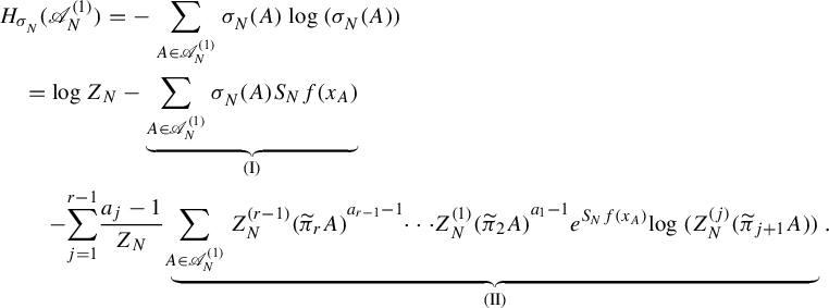 $$ \begin{align*} & H_{\sigma_N^{}}(\mathscr{A}^{(1)}_N) = - \sum_{A \in \mathscr{A}^{(1)}_N} \sigma_N^{}(A) \log{(\sigma_N^{}(A))} \\ &\quad = \log{Z_N} - \underbrace{\sum_{A \in \mathscr{A}^{(1)}_N} \sigma_N^{}(A) S_N f(x_A)}_{(\mathrm{I})} \\ &\qquad - \!\sum_{j=1}^{r-1}\!\frac{a_j-1}{Z_N} \underbrace{\!\sum_{A \in \mathscr{A}^{(1)}_N} {Z_N^{(r-1)}(\widetilde{\pi}_r A)}^{a_{r-1}-1}\!\cdots\! {Z_N^{(1)}(\widetilde{\pi}_2 A)}^{a_{1}-1} e^{S_N f(x_A)}\!\log{(Z_N^{(j)}(\widetilde{\pi}_{j+1} A) )}}_{(\mathrm{I}\mathrm{I})}. \end{align*} $$
For term
 $(\mathrm {I})$
, we have
$(\mathrm {I})$
, we have
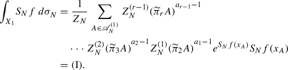 $$ \begin{align*} \int_{X_1} \! S_N f\,d\sigma_N^{} &= \frac{1}{Z_N} \sum_{A \in \mathscr{A}^{(1)}_N} {Z_N^{(r-1)}(\widetilde{\pi}_{r}A)}^{a_{r-1}-1}\\ &\quad \cdots {Z_N^{(2)}(\widetilde{\pi}_3 A)}^{a_{2}-1}{Z_N^{(1)}(\widetilde{\pi}_2 A)}^{a_{1}-1}e^{S_N f(x_A)} S_N f(x_A) \\ &= (\mathrm{I}). \end{align*} $$
We will show that
 $(\mathrm {I}\mathrm {I}) = W_N^{(j)}$
. Let
$(\mathrm {I}\mathrm {I}) = W_N^{(j)}$
. Let
 $A' \in \mathscr {A}^{(j+1)}_N$
. Then any
$A' \in \mathscr {A}^{(j+1)}_N$
. Then any
 $A \in \mathscr {A}^{(1)}_N(A')$
satisfies
$A \in \mathscr {A}^{(1)}_N(A')$
satisfies
 $\widetilde {\pi }_{j+1} A = A'$
. Hence,
$\widetilde {\pi }_{j+1} A = A'$
. Hence,
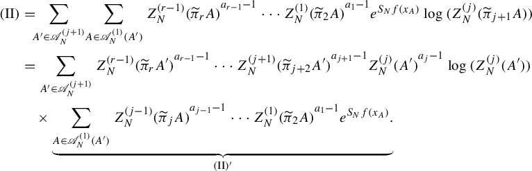 $$ \begin{align*} (\mathrm{I}\mathrm{I}) &=\!\!\sum_{A' \in \mathscr{A}^{(j+1)}_N}\! \sum_{A \in \mathscr{A}^{(1)}_N(A')} {Z_N^{(r-1)}(\widetilde{\pi}_r A)}^{a_{r-1}-1} \cdots {Z_N^{(1)}(\widetilde{\pi}_2 A)}^{a_{1}-1}e^{S_N f(x_A)} \log{(Z_N^{(j)}(\widetilde{\pi}_{j+1} A))} \\ &=\sum_{A' \in \mathscr{A}^{(j+1)}_N} {Z_N^{(r-1)}(\widetilde{\pi}_r A')}^{a_{r-1}-1} \cdots {Z_N^{(j+1)}(\widetilde{\pi}_{j+2} A')}^{a_{j+1}-1} {Z_N^{(j)}(A')}^{a_{j}-1} \log{(Z_N^{(j)} (A'))} \\ &\quad \times \underbrace{\sum_{A \in \mathscr{A}^{(1)}_N(A')} {Z_N^{(j-1)}(\widetilde{\pi}_j A)}^{a_{j-1}-1} \cdots {Z_N^{(1)}(\widetilde{\pi}_2 A)}^{a_{1}-1}e^{S_N f(x_A)}.}_{(\mathrm{I}\mathrm{I})'} \end{align*} $$
The term
 $(\mathrm {I}\mathrm {I})'$
can be calculated similarly to how we showed
$(\mathrm {I}\mathrm {I})'$
can be calculated similarly to how we showed
 $\sigma _N^{}(X_1)=1$
. Namely,
$\sigma _N^{}(X_1)=1$
. Namely,
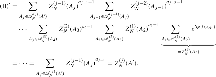 $$ \begin{align*} (\mathrm{I}\mathrm{I})' &= \sum_{A_j \in \mathscr{A}^{(j)}_N(A')} {Z_N^{(j-1)}(A_j)}^{a_{j-1}-1} \hspace{-10pt} \sum_{A_{j-1} \in \mathscr{A}^{(j-1)}_N(A_j)} {Z_N^{(j-2)}(A_{j-1})}^{a_{j-2}-1} \\ &\quad\cdots \sum_{A_3 \in \mathscr{A}^{(3)}_N(A_4)} Z_N^{(2)}(A_3)^{a_2-1} \sum_{A_2 \in \mathscr{A}^{(2)}_N(A_3)} {Z_N^{(1)}(A_2)}^{a_{1}-1} \underbrace{\sum_{A_1 \in \mathscr{A}^{(1)}_N(A_2)} e^{S_N f(x_{A_1})}}_{= Z_N^{(1)}(A_2)}\\ &= \cdots = \sum_{A_j \in \mathscr{A}^{(j)}_N(A')} {Z_N^{(j-1)}(A_j)}^{a_{j-1}} = Z^{(j)}_N(A'). \end{align*} $$
Thus, we get
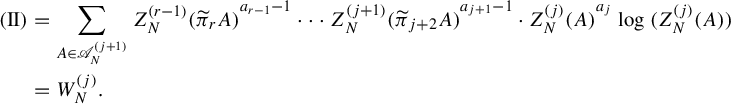 $$ \begin{align*} (\mathrm{I}\hspace{-0.5pt}\mathrm{I}) &= \sum_{A \in \mathscr{A}^{(j+1)}_N} {Z_N^{(r-1)}(\widetilde{\pi}_r A)}^{a_{r-1}-1} \cdots {Z_N^{(j+1)}(\widetilde{\pi}_{j+2} A)}^{a_{j+1}-1} \cdot {Z_N^{(j)}(A)}^{a_{j}} \log{( Z_N^{(j)}(A) )} \\ &= W_N^{(j)}. \end{align*} $$
This completes the proof of the first assertion.
Next, let
 $2 \leq i \leq r$
. For any
$2 \leq i \leq r$
. For any
 $A \in \mathscr {A}^{(i)}_N$
,
$A \in \mathscr {A}^{(i)}_N$
,
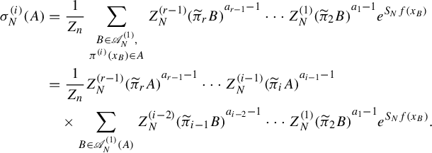 $$ \begin{align*} \sigma_N^{(i)}(A)&= \frac{1}{Z_n} \sum_{\substack{B \in \mathscr{A}^{(1)}_N, \\ \pi^{(i)} (x_B) \in A}} {Z_N^{(r-1)}(\widetilde{\pi}_r B)}^{a_{r-1}-1} \cdots {Z_N^{(1)}(\widetilde{\pi}_2 B)}^{a_{1}-1}e^{S_N f(x_B)}\\ &=\frac{1}{Z_n} {Z_N^{(r-1)}(\widetilde{\pi}_r A)}^{a_{r-1}-1} \cdots {Z_N^{(i-1)}(\widetilde{\pi}_i A)}^{a_{i-1}-1} \\ &\quad \times \sum_{B \in \mathscr{A}^{(1)}_N(A)} {Z_N^{(i-2)}(\widetilde{\pi}_{i-1} B)}^{a_{i-2}-1} \cdots {Z_N^{(1)}(\widetilde{\pi}_2 B)}^{a_{1}-1}e^{S_N f(x_B)}. \end{align*} $$
As in the evaluation of term
 $(\mathrm {I}\hspace {-0.5pt}\mathrm {I})'$
, we have
$(\mathrm {I}\hspace {-0.5pt}\mathrm {I})'$
, we have
 $$ \begin{align*} \sum_{B \in \mathscr{A}^{(1)}_N(A)} {Z_N^{(i-2)}(\widetilde{\pi}_{i-1} B)}^{a_{i-2}-1} \cdots {Z_N^{(1)}(\widetilde{\pi}_2 B)}^{a_{1}-1}e^{S_N f(x_B)} = {Z^{(i-1)}_N(A)}^{a_{i-1}}.\end{align*} $$
Hence,
 $$ \begin{align*} \sigma_N^{(i)}(A) &= \frac{1}{Z_n} {Z_N^{(r-1)}(\widetilde{\pi}_r A)}^{a_{r-1}-1} \cdots {Z_N^{(i)}(\widetilde{\pi}_{i+1} A)}^{a_{i}-1} {Z_N^{(i-1)}(A)}^{a_{i-1}}. \end{align*} $$
Therefore,
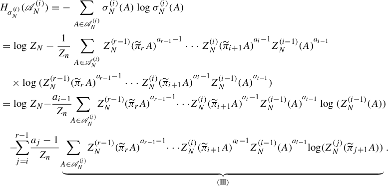 $$ \begin{align*} &H_{\sigma_N^{(i)}}(\mathscr{A}^{(i)}_N) = - \sum_{A \in \mathscr{A}^{(i)}_N} \sigma_N^{(i)}(A) \log{\sigma_N^{(i)}(A)} \\ &=\log{Z_N} - \frac{1}{Z_n} \sum_{A \in \mathscr{A}^{(i)}_N} {Z_N^{(r-1)}(\widetilde{\pi}_r A)}^{a_{r-1}-1} \cdots {Z_N^{(i)}(\widetilde{\pi}_{i+1} A)}^{a_{i}-1} {Z_N^{(i-1)}(A)}^{a_{i-1}} \\ &\quad \times \log{( {Z_N^{(r-1)}(\widetilde{\pi}_r A)}^{a_{r-1}-1} \cdots {Z_N^{(i)}(\widetilde{\pi}_{i+1} A)}^{a_{i}-1} {Z_N^{(i-1)}(A)}^{a_{i-1}})}\\ &=\log{Z_N}\!-\! \frac{a_{i-1}}{Z_n}\!\!\sum_{A \in \mathscr{A}^{(i)}_N}\! {Z_N^{(r-1)}(\widetilde{\pi}_r A)}^{a_{r-1}-1}\! \cdots\! {Z_N^{(i)}(\widetilde{\pi}_{i+1} A)}^{a_{i}-1} {Z_N^{(i-1)}(A)}^{a_{i-1}} \log{( Z_N^{(i-1)}(A))} \\ &\quad\! -\!\! \sum_{j=i}^{r-1}\! \frac{a_{j}-1}{Z_n} \underbrace{\!\sum_{A \in \mathscr{A}^{(i)}_N}\!{Z_N^{(r-1)}(\widetilde{\pi}_r A)}^{a_{r-1}-1}\! \cdots\! {Z_N^{(i)}(\widetilde{\pi}_{i+1} A)}^{a_{i}-1} {Z_N^{(i-1)}(A)}^{a_{i-1}}\! \log\! {( Z_N^{(j)}(\widetilde{\pi}_{j+1} A) )}}_{(\mathrm{I}\hspace{-0.5pt}\mathrm{I}\hspace{-0.5pt}\mathrm{I})}. \end{align*} $$
Note that we can calculate term
 $(\mathrm {I}\hspace {-0.5pt}\mathrm {I}\hspace {-0.5pt}\mathrm {I})$
as
$(\mathrm {I}\hspace {-0.5pt}\mathrm {I}\hspace {-0.5pt}\mathrm {I})$
as
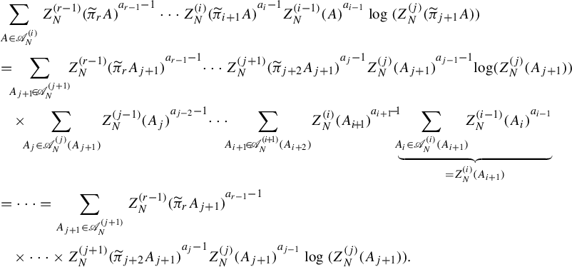 $$ \begin{align*} & \!\sum_{A \in \mathscr{A}^{(i)}_N} {Z_N^{(r-1)}(\widetilde{\pi}_r A)}^{a_{r-1}-1} \cdots {Z_N^{(i)}(\widetilde{\pi}_{i+1} A)}^{a_{i}-1} {Z_N^{(i-1)}(A)}^{a_{i-1}} \log{( Z_N^{(j)}(\widetilde{\pi}_{j+1} A))} \\&\!=\!\!\sum_{A_{j+1} \!\in\! \mathscr{A}^{(j+1)}_N}\!\! {Z_N^{(r-1)}(\widetilde{\pi}_r A_{j+1})}^{a_{r-1}-1} \!\cdots {Z_N^{(j+1)}(\widetilde{\pi}_{j+2} A_{j+1})}^{a_j-1} {Z_N^{(j)}(A_{j+1})}^{a_{j-1}-1}\!\log\!{( Z_N^{(j)}(A_{j+1}))} \\&\!\quad\times\!\! \sum_{A_j \in \mathscr{A}^{(j)}_N(A_{j+1})}\! {Z^{(j-1)}_N(A_j)}^{a_{j-2}-1}\! \cdots \!\! \sum_{A_{i+1}\! \in\! \mathscr{A}^{(i\!+\!1)}_N(A_{i+2})}\! {Z^{(i)}_N(A_{i\!+\!1})}^{a_{i+1}\!-\!1}\!\! \underbrace{\!\sum_{A_i \in \mathscr{A}^{(i)}_N(A_{i+1})} \!\!{Z^{(i-1)}_N(A_i)}^{a_{i-1}}}_{= Z^{(i)}_N(A_{i+1})}\\&\!= \cdots = \sum_{A_{j+1} \in \mathscr{A}^{(j+1)}_N} {Z_N^{(r-1)}(\widetilde{\pi}_r A_{j+1})}^{a_{r-1}-1} \\&\!\quad \times \cdots \times {Z_N^{(j+1)}(\widetilde{\pi}_{j+2} A_{j+1})}^{a_j-1} {Z_N^{(j)}(A_{j+1})}^{a_{j-1}} \log{( Z_N^{(j)}(A_{j+1}))}. \end{align*} $$
We conclude that
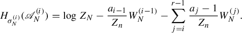 $$ \begin{align*} H_{\sigma_N^{(i)}}(\mathscr{A}^{(i)}_N) = \log{Z_N} - \frac{a_{i-1}}{Z_n} W_N^{(i-1)} - \sum_{j=i}^{r-1} \frac{a_{j}-1}{Z_n} W_N^{(j)}. \end{align*} $$
This completes the proof of the claim.
By this claim,
 $$ \begin{align*} \sum_{i=1}^r w_i H_{\sigma_N^{(i)}}\! (\mathscr{A}^{(i)}_N) \!+\! w_1 \int_{X_1} \! S_N f\,d\mu &= \log{Z_N}\! -\! \sum_{i=2}^r \frac{w_i a_{i-1}}{Z_n} W_N^{(i-1)} \!-\! \sum_{i=1}^{r-1} \sum_{j=i}^{r-1} \frac{w_i(a_{j}\!-\!1)}{Z_n} W_N^{(j)}.\end{align*} $$
However, we have
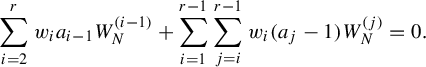 $$ \begin{align*} \sum_{i=2}^r w_i a_{i-1} W_N^{(i-1)} + \sum_{i=1}^{r-1} \sum_{j=i}^{r-1} w_i(a_{j}-1) W_N^{(j)} = 0. \end{align*} $$
Indeed, the coefficient of
 $W_N^{(k)}$
(
$W_N^{(k)}$
(
 $1 \leq k \leq r-1$
) is
$1 \leq k \leq r-1$
) is
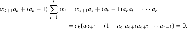 $$ \begin{align*} w_{k+1}a_k + (a_k - 1) \sum_{i=1}^k w_i &= w_{k+1}a_k + (a_k - 1) a_k a_{k+1} \cdots a_{r-1} \\ &= a_k \{ w_{k+1} - (1-a_k) a_{k+1} a_{k+2} \cdots a_{r-1} \} = 0. \end{align*} $$
Thus, we have
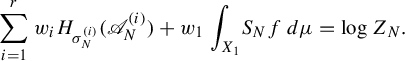 $$ \begin{align} \sum_{i=1}^r w_i H_{\sigma_N^{(i)}} (\mathscr{A}^{(i)}_N) + w_1 \int_{X_1} \! S_N f\,d\mu = \log{Z_N}. \end{align} $$
Let
 $\mu ^{(i)} = {\pi ^{(i-1)}}_* \mu $
and
$\mu ^{(i)} = {\pi ^{(i-1)}}_* \mu $
and
 $\mu ^{(i)}_N = {\pi ^{(i-1)}}_* \mu _N^{}$
.
$\mu ^{(i)}_N = {\pi ^{(i-1)}}_* \mu _N^{}$
.
Lemma 4.3. Let N and M be natural numbers. For any
 $1 \leq i \leq r$
,
$1 \leq i \leq r$
,
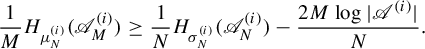 $$ \begin{align*} \frac{1}{M} H_{\mu^{(i)}_N} (\mathscr{A}^{(i)}_M) \geq \frac{1}{N} H_{\sigma_N^{(i)}}(\mathscr{A}^{(i)}_N) - \frac{2M \log{ \lvert {\mathscr{A}^{(i)}} \rvert }}{N}. \end{align*} $$
Here,
 $ \lvert {\mathscr {A}^{(i)}} \rvert $
is the number of elements in
$ \lvert {\mathscr {A}^{(i)}} \rvert $
is the number of elements in
 $\mathscr {A}^{(i)}$
.
$\mathscr {A}^{(i)}$
.
Suppose this is true, and let N and M be natural numbers. Together with equation (4.1), we obtain the following evaluation:
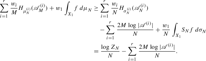 $$ \begin{align*} \sum_{i=1}^r \frac{w_i}{M} H_{\mu^{(i)}_N}(\mathscr{A}^{(i)}_M) + w_1 \int_{X_1} \! f\,d\mu_N^{} & \geq \sum_{i=1}^r \frac{w_i}{N} H_{\sigma_N^{(i)}}(\mathscr{A}^{(i)}_N) \\ &\quad -\sum_{i=1}^r \frac{2M \log{ \lvert {\mathscr{A}^{(i)}} \rvert }}{N} + \frac{w_1}{N} \int_{X_1} \! S_N f\,d\sigma_N^{} \\ &= \frac{\log{Z_N}}{N} - \sum_{i=1}^r \frac{2M \log{ \lvert {\mathscr{A}^{(i)}} \rvert }}{N}. \end{align*} $$
Let
 $N = N_k \to \infty $
along the sub-sequence
$N = N_k \to \infty $
along the sub-sequence
 $(N_k)$
for which
$(N_k)$
for which
 $\mu _{N_k}^{} \rightharpoonup \mu $
. This yields
$\mu _{N_k}^{} \rightharpoonup \mu $
. This yields
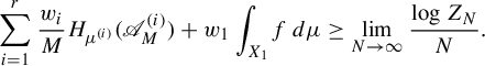 $$ \begin{align*} \sum_{i=1}^r \frac{w_i}{M} H_{\mu^{(i)}}(\mathscr{A}^{(i)}_M) + w_1 \int_{X_1} \! f\,d\mu \geq \lim_{N \to \infty} \frac{\log{Z_N}}{N}. \end{align*} $$
We let
 $M \to \infty $
and get
$M \to \infty $
and get
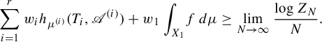 $$ \begin{align*} \sum_{i=1}^r w_i h_{\mu^{(i)}}(T_i, \mathscr{A}^{(i)}) + w_1 \int_{X_1} \! f\,d\mu \geq \lim_{N \to \infty} \frac{\log{Z_N}}{N}. \end{align*} $$
Hence,
 $$ \begin{align*} P^{\boldsymbol{a}}_{\mathrm{var}}(f) \geq P^{\boldsymbol{a}}(f). \end{align*} $$
We are left to prove Lemma 4.3.
Proof of Lemma 4.3
This statement appears in the proof of variational principle in [Reference WaltersWal82, Theorem 8.6], and Tsukamoto also proves it in [Reference TsukamotoTsu22, Claim 6.3]. The following proof is taken from the latter. We will explain for
 $i=1$
; the same argument works for all i.
$i=1$
; the same argument works for all i.
Let
 $\mathscr {A} = \mathscr {A}^{(1)}$
. Recall that
$\mathscr {A} = \mathscr {A}^{(1)}$
. Recall that
 $\mu _N^{} = ({1}/{N}) \sum _{k=0}^{N-1} {{T_1}^k}_* \sigma _N^{}$
. Since the entropy function is concave (Lemma 3.5), we have
$\mu _N^{} = ({1}/{N}) \sum _{k=0}^{N-1} {{T_1}^k}_* \sigma _N^{}$
. Since the entropy function is concave (Lemma 3.5), we have
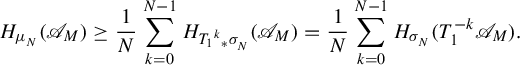 $$ \begin{align*} H_{\mu_N^{}}(\mathscr{A}_M) \geq \frac{1}{N} \sum_{k=0}^{N-1} H_{{{T_1}^k}_* \sigma_N^{}}(\mathscr{A}_M) = \frac{1}{N} \sum_{k=0}^{N-1} H_{\sigma_N^{}}(T_1^{-k}\mathscr{A}_M). \end{align*} $$
Let
 $N = qM + r$
with
$N = qM + r$
with
 $0 \leq r < M$
, then
$0 \leq r < M$
, then
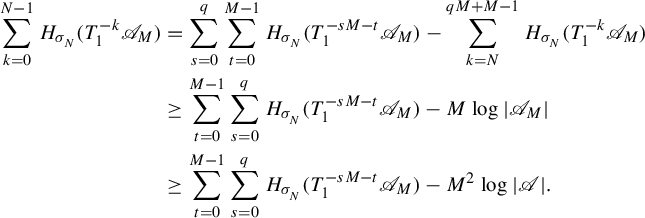 $$ \begin{align} \sum_{k=0}^{N-1} H_{\sigma_N^{}}(T_1^{-k}\mathscr{A}_M) &= \sum_{s=0}^q \sum_{t=0}^{M-1} H_{\sigma_N^{}}(T_1^{-sM-t}\mathscr{A}_M) - \sum_{k=N}^{qM+M-1} H_{\sigma_N^{}}(T_1^{-k}\mathscr{A}_M) \nonumber \\ &\geq \sum_{t=0}^{M-1} \sum_{s=0}^q H_{\sigma_N^{}}(T_1^{-sM-t}\mathscr{A}_M) - M \log{ \left\lvert {\mathscr{A}_M} \right\rvert } \nonumber \\ &\geq \sum_{t=0}^{M-1} \sum_{s=0}^q H_{\sigma_N^{}}(T_1^{-sM-t}\mathscr{A}_M) - M^2 \log{ \left\lvert {\mathscr{A}} \right\rvert }. \end{align} $$
We will evaluate
 $\sum _{s=0}^q H_{\sigma _N^{}}(T_1^{-sM-t}\mathscr {A}_M)$
from below for each
$\sum _{s=0}^q H_{\sigma _N^{}}(T_1^{-sM-t}\mathscr {A}_M)$
from below for each
 $0 \leq t \leq M-1$
. First, observe that
$0 \leq t \leq M-1$
. First, observe that
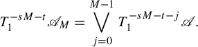 $$ \begin{align*} T_1^{-sM-t}\mathscr{A}_M = \bigvee_{j=0}^{M-1} T_1^{-sM-t-j}\mathscr{A}. \end{align*} $$
We have
 $$ \begin{align*} \{ sM + t + j | 0 \leq s \leq q, 0 \leq j \leq M - 1 \} = \{ t, t + 1, \ldots, t + qM + M - 1 \} \end{align*} $$
without multiplicity. Therefore,
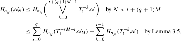 $$ \begin{align*} H_{\sigma_N^{}}(\mathscr{A}_N) &\leq H_{\sigma_N^{}}\bigg( \bigvee_{k=0}^{t+(q+1)M-1} T_1^{-k} \mathscr{A} \bigg) \quad \text{by } N <t+(q+1)M \\ &\leq \sum_{s=0}^q H_{\sigma_N^{}}(T_1^{-sM-t}\mathscr{A}_M) + \sum_{k=0}^{t-1}H_{\sigma_N^{}}(T_1^{-k}\mathscr{A}) \quad \text{by Lemma 3.5}. \end{align*} $$
This implies
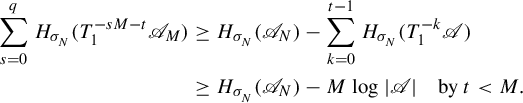 $$ \begin{align*} \sum_{s=0}^q H_{\sigma_N^{}}(T_1^{-sM-t}\mathscr{A}_M) &\geq H_{\sigma_N^{}}(\mathscr{A}_N) - \sum_{k=0}^{t-1}H_{\sigma_N^{}}(T_1^{-k}\mathscr{A}) \\ &\geq H_{\sigma_N^{}}(\mathscr{A}_N) - M \log{ \left\lvert {\mathscr{A}} \right\rvert } \quad \text{by } t < M. \end{align*} $$
Now, we sum over t and obtain
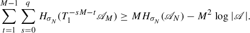 $$ \begin{align*} \sum_{t=1}^{M-1} \sum_{s=0}^q H_{\sigma_N^{}}(T_1^{-sM-t}\mathscr{A}_M) &\geq M H_{\sigma_N^{}}(\mathscr{A}_N) - M^2 \log{ \left\lvert {\mathscr{A}} \right\rvert }.\end{align*} $$
Combining with equation (4.2), this implies
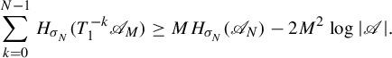 $$ \begin{align*} \sum_{k=0}^{N-1} H_{\sigma_N^{}}(T_1^{-k}\mathscr{A}_M) \geq M H_{\sigma_N^{}}(\mathscr{A}_N) - 2M^2 \log{ \left\lvert {\mathscr{A}} \right\rvert }. \end{align*} $$
It follows that
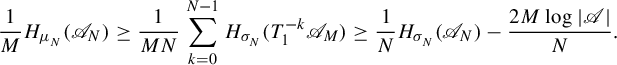 $$ \begin{align*} \frac{1}{M} H_{\mu_N^{}}(\mathscr{A}_N) \geq \frac{1}{MN} \sum_{k=0}^{N-1} H_{\sigma_N^{}}(T_1^{-k}\mathscr{A}_M) \geq \frac{1}{N} H_{\sigma_N^{}}(\mathscr{A}_N) - \frac{2M \log{ \left\lvert {\mathscr{A}} \right\rvert }}{N}.\\[-39pt] \end{align*} $$
This completes the proof of Theorem 4.1.
5. Proof of
$P^{\boldsymbol {a}}_{\mathrm {var}}(f) \leq P^{\boldsymbol {a}}(f)$

It seems difficult to implement the zero-dimensional trick to prove
 $P^{\boldsymbol {a}}_{\mathrm {var}}(f) \leq P^{\boldsymbol {a}}(f)$
. Hence, the proof is more complicated.
$P^{\boldsymbol {a}}_{\mathrm {var}}(f) \leq P^{\boldsymbol {a}}(f)$
. Hence, the proof is more complicated.
Theorem 5.1. Suppose that
 $(X_i, T_i)$
(
$(X_i, T_i)$
(
 $i=1, 2, \ldots , r$
) are dynamical systems and
$i=1, 2, \ldots , r$
) are dynamical systems and
 $\pi _i: X_i \rightarrow X_{i+1}\ (i=1, 2, \ldots , r-1)$
are factor maps. Then we have
$\pi _i: X_i \rightarrow X_{i+1}\ (i=1, 2, \ldots , r-1)$
are factor maps. Then we have
 $$ \begin{align*} P^{\boldsymbol{a}}_{\mathrm{var}}(f) \leq P^{\boldsymbol{a}}(f) \end{align*} $$
for any continuous function
 $f: X_1 \rightarrow \mathbb {R}$
.
$f: X_1 \rightarrow \mathbb {R}$
.
Proof. Take and fix
 $\mu \in \mathscr {M}^{T_1}(X_1)$
. Let
$\mu \in \mathscr {M}^{T_1}(X_1)$
. Let
 $\mu _i= {\pi ^{(i-1)}}_* \mu $
. We need to prove
$\mu _i= {\pi ^{(i-1)}}_* \mu $
. We need to prove
 $$ \begin{align*} \sum_{i=1}^r w_i h_{\mu_i}(T_i) + w_1 \int_{X_1} f\,d\mu \leq P^{\boldsymbol{a}}(f, \boldsymbol{T}). \end{align*} $$
However, the following argument assures that giving an evaluation up to a constant is sufficient: suppose there is a positive number C which does not depend on f nor
 $(T_i)_i$
satisfying
$(T_i)_i$
satisfying
 $$ \begin{align} \sum_{i=1}^r w_i h_{\mu_i}(T_i) + w_1 \int_{X_1} f\,d\mu \leq P^{\boldsymbol{a}}(f, \boldsymbol{T}) + C. \end{align} $$
Applying this to
 $S_mf$
and
$S_mf$
and
 $\boldsymbol {T}^m = ({T_i}^m)_i$
for
$\boldsymbol {T}^m = ({T_i}^m)_i$
for
 $m \in \mathbb {N}$
yields
$m \in \mathbb {N}$
yields
 $$ \begin{align*} \sum_{i=1}^r w_i h_{\mu_i}({T_i}^m) + w_1 \int_{X_1} \! S_mf\,d\mu \leq P^{\boldsymbol{a}}(S_mf, \boldsymbol{T}^m) + C. \end{align*} $$
We employ Lemma 3.3 and get
 $$ \begin{align*} m \sum_{i=1}^r w_i h_{\mu_i}(T_i) + m w_1 \int_{X_1} \! f\,d\mu \leq mP^{\boldsymbol{a}}(f, \boldsymbol{T}) + C. \end{align*} $$
Divide by m and let
 $m \to \infty $
. We obtain the desired inequality
$m \to \infty $
. We obtain the desired inequality
 $$ \begin{align*} \sum_{i=1}^r w_i h_{\mu_i}(T_i) + w_1 \int_{X_1} \! f\,d\mu \leq P^{\boldsymbol{a}}(f, \boldsymbol{T}). \end{align*} $$
Therefore, we only need to prove inequality (5.1).
Let
 $\mathscr {A}^{(i)} = \{ A^{(i)}_1, A^{(i)}_2, \ldots , A^{(i)}_{m_i} \}$
be an arbitrary partition of
$\mathscr {A}^{(i)} = \{ A^{(i)}_1, A^{(i)}_2, \ldots , A^{(i)}_{m_i} \}$
be an arbitrary partition of
 $X_i$
for each i. We will prove
$X_i$
for each i. We will prove
 $$ \begin{align*} \sum_{i=1}^r w_i h_{\mu_i}(T_i, \mathscr{A}^{(i)}) + w_1 \int_{X_1} \! f\,d\mu \leq P^{\boldsymbol{a}}(f, \boldsymbol{T}) + C. \end{align*} $$
We start by approximating elements of
 $\mathscr {A}^{(i)}$
with compact sets using backward induction. For
$\mathscr {A}^{(i)}$
with compact sets using backward induction. For
 $1\leq i \leq r$
, let
$1\leq i \leq r$
, let
 $$ \begin{align*} \Lambda_i^{0} &= \{0, 1, \ldots, m_r\} \times \{0, 1, \ldots, m_{r-1}\} \times \cdots \times \{0, 1, \ldots, m_{i+1}\} \times \{0, 1, \ldots, m_i\},\\\Lambda_i &= \{0, 1, \ldots, m_r\} \times \{0, 1, \ldots, m_{r-1}\} \times \cdots \times \{0, 1, \ldots, m_{i+1}\} \times \{1, 2, \ldots, m_i\}.\end{align*} $$
We will denote an element
 $(j_r, j_{r-1}, \ldots , j_i)$
in
$(j_r, j_{r-1}, \ldots , j_i)$
in
 $\Lambda _i^{0}$
or
$\Lambda _i^{0}$
or
 $\Lambda _i$
by
$\Lambda _i$
by
 $j_r j_{r-1} \cdots j_i$
. For each
$j_r j_{r-1} \cdots j_i$
. For each
 $A^{(r)}_j \in \mathscr {A}^{(r)}$
, take a compact set
$A^{(r)}_j \in \mathscr {A}^{(r)}$
, take a compact set
 $C^{(r)}_j \subset A^{(r)}_j$
such that
$C^{(r)}_j \subset A^{(r)}_j$
such that
 $$ \begin{align*} \log{m_r} \cdot \sum_{j=1}^{m_r} \mu_r\big(A^{(r)}_j \setminus C^{(r)}_j\big) < 1. \end{align*} $$
Define
 $C^{(r)}_0$
as the remainder of
$C^{(r)}_0$
as the remainder of
 $X_r$
, which may not be compact:
$X_r$
, which may not be compact:
 $$ \begin{align*} C^{(r)}_0 = \bigcup_{j=1}^{m_r} A^{(r)}_j \setminus C^{(r)}_j = X_r \setminus \bigcup_{j=1}^{m_r} C^{(r)}_j. \end{align*} $$
Then
 $\mathscr {C}^{(r)} := \{ C^{(r)}_0, C^{(r)}_1, \ldots , C^{(r)}_{m_r} \}$
is a measurable partition of
$\mathscr {C}^{(r)} := \{ C^{(r)}_0, C^{(r)}_1, \ldots , C^{(r)}_{m_r} \}$
is a measurable partition of
 $X_r$
.
$X_r$
.
Next, consider the partition
 $\pi _{r-1}^{-1}(\mathscr {C}^{(r)}) \vee \mathscr {A}^{(r-1)}$
of
$\pi _{r-1}^{-1}(\mathscr {C}^{(r)}) \vee \mathscr {A}^{(r-1)}$
of
 $X_{r-1}$
. For
$X_{r-1}$
. For
 $j_r j_{r-1} \in \Lambda _{r-1}$
, let
$j_r j_{r-1} \in \Lambda _{r-1}$
, let
 $$ \begin{align*} B^{(r-1)}_{j_r j_{r-1}} = \pi_{r-1}^{-1}(C^{(r)}_{j_r}) \cap A^{(r-1)}_{j_{r-1}}. \end{align*} $$
Then
 $$ \begin{align*} \pi_{r-1}^{-1}(\mathscr{C}^{(r)}) \vee \mathscr{A}^{(r-1)} = \{ B^{(r-1)}_{j_r j_{r-1}} | j_r j_{r-1} \in \Lambda_{r-1} \}, \end{align*} $$
and for each
 $j_r \in \Lambda _r^0$
,
$j_r \in \Lambda _r^0$
,
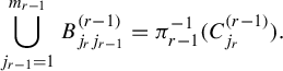 $$ \begin{align*} \bigcup_{j_{r-1}=1}^{m_{r-1}} B^{(r-1)}_{j_r j_{r-1}} = \pi_{r-1}^{-1}(C^{(r-1)}_{j_r}). \end{align*} $$
For each
 $j_rj_{r-1} \in \Lambda _{r-1}$
, take a compact set
$j_rj_{r-1} \in \Lambda _{r-1}$
, take a compact set
 $C^{(r-1)}_{j_r j_{r-1}} \subset B^{(r-1)}_{j_r j_{r-1}}$
(which could be empty) such that
$C^{(r-1)}_{j_r j_{r-1}} \subset B^{(r-1)}_{j_r j_{r-1}}$
(which could be empty) such that
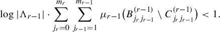 $$ \begin{align*} \log{ \left\lvert {\Lambda_{r-1}} \right\rvert } \cdot \sum_{j_r = 0}^{m_r} \sum_{j_{r-1}=1}^{m_{r-1}} \mu_{r-1}\big(B^{(r-1)}_{j_r j_{r-1}} \setminus C^{(r-1)}_{j_r j_{r-1}}\big) < 1. \end{align*} $$
Define
 $C^{(r-1)}_{j_r 0}$
as the remainder of
$C^{(r-1)}_{j_r 0}$
as the remainder of
 $\pi _{r-1}^{-1}(C^{(r)}_{j_r})$
:
$\pi _{r-1}^{-1}(C^{(r)}_{j_r})$
:
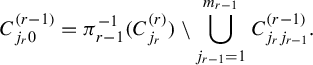 $$ \begin{align*} C^{(r-1)}_{j_r 0} = \pi_{r-1}^{-1}(C^{(r)}_{j_r}) \setminus \bigcup_{j_{r-1}=1}^{m_{r-1}} C^{(r-1)}_{j_r j_{r-1}}. \end{align*} $$
Then
 $\mathscr {C}^{(r-1)} = \{ C^{(r-1)}_{j_r j_{r-1}} | j_r j_{r-1} \in \Lambda _{r-1}^{0} \} $
is a measurable partition of
$\mathscr {C}^{(r-1)} = \{ C^{(r-1)}_{j_r j_{r-1}} | j_r j_{r-1} \in \Lambda _{r-1}^{0} \} $
is a measurable partition of
 $X_{r-1}$
.
$X_{r-1}$
.
Continue in this manner, and suppose we have obtained the partition
 $\mathscr {C}^{(k)} = \{ C^{(k)}_J | J \in \Lambda _k^{0} \}$
of
$\mathscr {C}^{(k)} = \{ C^{(k)}_J | J \in \Lambda _k^{0} \}$
of
 $X_k$
for
$X_k$
for
 $k = i+1, i+2, \ldots , r$
. We will define
$k = i+1, i+2, \ldots , r$
. We will define
 $\mathscr {C}^{(i)}$
. Each element in
$\mathscr {C}^{(i)}$
. Each element in
 $\pi _i^{-1}(\mathscr {C}^{(i+1)}) \vee \mathscr {A}^{(i)}$
can be expressed using
$\pi _i^{-1}(\mathscr {C}^{(i+1)}) \vee \mathscr {A}^{(i)}$
can be expressed using
 $J' \in \Lambda _{i+1}^0$
and
$J' \in \Lambda _{i+1}^0$
and
 $j_i \in \{1,2, \ldots , m_i\}$
by
$j_i \in \{1,2, \ldots , m_i\}$
by
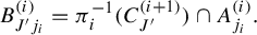 $$ \begin{align*} B_{J'j_i}^{(i)} = \pi_i^{-1}(C_{J'}^{(i+1)}) \cap A_{j_i}^{(i)}. \end{align*} $$
Choose a compact set
 $C_J^{(i)} \subset B_J^{(i)}$
for each
$C_J^{(i)} \subset B_J^{(i)}$
for each
 $J \in \Lambda _{i}$
so that
$J \in \Lambda _{i}$
so that
 $$ \begin{align*} \log{ \left\lvert {\Lambda_i} \right\rvert } \cdot \sum_{J' \in \Lambda_{i+1}^0} \sum_{j_i=1}^{m_i} \mu_i \big( B^{(i)}_{J'j_i} \setminus C^{(i)}_{J'j_i} \big) < 1. \end{align*} $$
Finally, for
 $J' \in \Lambda _{j+1}^{0}$
, let
$J' \in \Lambda _{j+1}^{0}$
, let
 $$ \begin{align*} C_{J'0}^{(i)} = \pi_i^{-1}(C_{J'}^{(i+1)}) \setminus \bigcup_{j_i=1}^{m_i} C_{J'j_i}^{(i)}. \end{align*} $$
Set
 $\mathscr {C}^{(i)} = \{ C^{(i)}_J | J \in \Lambda _i^{0} \}$
. This is a partition of
$\mathscr {C}^{(i)} = \{ C^{(i)}_J | J \in \Lambda _i^{0} \}$
. This is a partition of
 $X_i$
.
$X_i$
.
Lemma 5.2. For
 $\mathscr {C}^{(i)}$
constructed above, we have
$\mathscr {C}^{(i)}$
constructed above, we have
 $$ \begin{align*} h_{\mu_i}(T_i, \mathscr{A}^{(i)}) \leq h_{\mu_i}(T_i, \mathscr{C}^{(i)}) + 1. \end{align*} $$
Proof. By Lemma 3.5,
 $$ \begin{align*} h_{\mu_i}(T_i, \mathscr{A}^{(i)}) &\leq h_{\mu_i} \! (T_i, \mathscr{A}^{(i)} \vee \pi_i^{-1}(\mathscr{C}^{(i+1)})) \\ &\leq h_{\mu_i}(T_i, \mathscr{C}^{(i)}) + H_{\mu_i}( \mathscr{A}^{(i)} \vee \pi_i^{-1}(\mathscr{C}^{(i+1)}) | \mathscr{C}^{(i)}). \end{align*} $$
Since
 $C^{(i)}_J \subset B^{(i)}_J$
for
$C^{(i)}_J \subset B^{(i)}_J$
for
 $J \in \Lambda _i$
,
$J \in \Lambda _i$
,
 $$ \begin{align*} & H_{\mu_i}( \mathscr{A}^{(i)} \vee \pi_i^{-1}(\mathscr{C}^{(i+1)}) | \mathscr{C}^{(i)} ) \\ &\quad = - \sum_{\substack{J \in \Lambda_i^0 \\ \mu_i(C_J^{(i)}) \ne 0}} \mu_i(C_J^{(i)}) \sum_{K \in \Lambda_i} \frac{\mu_i(B_{K}^{(i)} \cap C_J^{(i)})}{\mu_i(C_J^{(i)})} \log{\bigg( \frac{\mu_i(B_{K}^{(i)} \cap C_J^{(i)})}{\mu_i(C_J^{(i)})} \bigg)} \\ &\quad= - \sum_{\substack{J' \in \Lambda_{i+1}^0 \\ \mu_i(C_{J'0}^{(i)}) \ne 0}} \mu_i(C_{J'0}^{(i)}) \sum_{j_i=1}^{m_i} \frac{\mu_i(B_{J' j_i}^{(i)} \cap C_{J'0}^{(i)})}{\mu_i(C_{J'0}^{(i)})} \log{\bigg( \frac{\mu_i(B_{J' j_i}^{(i)} \cap C_{J'0}^{(i)})}{\mu_i(C_{J'0}^{(i)})} \bigg)}. \end{align*} $$
By Lemma 3.4, we have
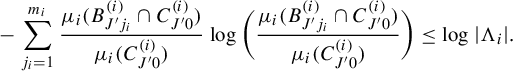 $$ \begin{align*} - \sum_{j_i=1}^{m_i} \frac{\mu_i(B_{J' j_i}^{(i)} \cap C_{J'0}^{(i)})}{\mu_i(C_{J'0}^{(i)})} \log{\bigg( \frac{\mu_i(B_{J' j_i}^{(i)} \cap C_{J'0}^{(i)})}{\mu_i(C_{J'0}^{(i)})} \bigg)} \leq \log{ \left\lvert {\Lambda_i} \right\rvert }. \end{align*} $$
Therefore,
 $$ \begin{align*}\hspace{-25pt} H_{\mu_i}( \mathscr{A}^{(i)} \vee \pi_i^{-1}(\mathscr{C}^{(i+1)}) | \mathscr{C}^{(i)} ) &\leq \log{ \left\lvert {\Lambda_i} \right\rvert } \sum_{J' \in \Lambda_{i+1}^0} \mu_i\bigg(\pi_i^{-1}(C_{J'}^{(i+1)}) \setminus \bigcup_{j_i=1}^{m_i} C_{J'j_i}^{(i)}\bigg) < 1.\\[-49pt] \end{align*} $$
Recall the definition of
 $\boldsymbol {w}$
in equation (2.1). We have
$\boldsymbol {w}$
in equation (2.1). We have
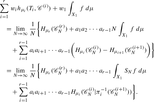 $$ \begin{align*} & \sum_{i=1}^r w_ih_{\mu_i}(T_i, \mathscr{C}^{(i)}) + w_1 \int_{X_1} f\,d\mu \\ &\quad = \lim_{N \to \infty} \frac{1}{N} \bigg\{ H_{\mu_r}(\mathscr{C}^{(r)}_N) + a_1a_2 \cdots a_{r-1} N \int_{X_1} f\,d\mu \\ &\qquad + \sum_{i=1}^{r-1} a_i a_{i+1} \cdots a_{r-1}\bigg(H_{\mu_i}(\mathscr{C}^{(i)}_N) - H_{\mu_{i+1}}(\mathscr{C}^{(i+1)}_N)\bigg) \bigg\}\\ &\quad= \lim_{N \to \infty} \frac{1}{N} \bigg\{ H_{\mu_r}(\mathscr{C}^{(r)}_N) + a_1a_2 \cdots a_{r-1} \int_{X_1} S_Nf\,d\mu \\ &\qquad + \sum_{i=1}^{r-1} a_i a_{i+1} \cdots a_{r-1} H_{\mu_i}(\mathscr{C}^{(i)}_N | \pi_i^{-1}(\mathscr{C}^{(i+1)}_N) ) \bigg\}. \end{align*} $$
Here, we used the relation
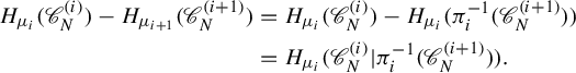 $$ \begin{align*} H_{\mu_i}(\mathscr{C}^{(i)}_N) - H_{\mu_{i+1}}(\mathscr{C}^{(i+1)}_N) &= H_{\mu_i}(\mathscr{C}^{(i)}_N) - H_{\mu_i}(\pi_i^{-1}(\mathscr{C}^{(i+1)}_N)) \\ &=H_{\mu_i}(\mathscr{C}^{(i)}_N | \pi_i^{-1}(\mathscr{C}^{(i+1)}_N)). \end{align*} $$
We fix N and evaluate from above the following terms using backward induction:
 $$ \begin{align} H_{\mu_r}(\mathscr{C}^{(r)}_N) + a_1a_2 \cdots a_{r-1} \int_{X_1} S_Nf\,d\mu + \sum_{i=1}^{r-1} a_i a_{i+1} \cdots a_{r-1} H_{\mu_i}(\mathscr{C}^{(i)}_N | \pi_i^{-1}(\mathscr{C}^{(i+1)}_N)). \end{align} $$
First, consider the term
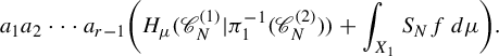 $$ \begin{align*}a_1a_2 \cdots a_{r-1} \bigg( H_{\mu}(\mathscr{C}^{(1)}_N | \pi_1^{-1}(\mathscr{C}^{(2)}_N)) + \int_{X_1} S_Nf\,d\mu \bigg). \end{align*} $$
For
 $C \in \mathscr {C}^{(i+1)}_N$
, let
$C \in \mathscr {C}^{(i+1)}_N$
, let
 $\mathscr {C}^{(i)}_N(C) = \{ D \in \mathscr {C}^{(i)}_N | \pi _i(D) \subset C \}$
, then by Lemma 3.4,
$\mathscr {C}^{(i)}_N(C) = \{ D \in \mathscr {C}^{(i)}_N | \pi _i(D) \subset C \}$
, then by Lemma 3.4,
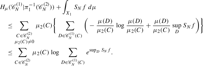 $$ \begin{align*} & H_{\mu}(\mathscr{C}^{(1)}_N | \pi_1^{-1}(\mathscr{C}^{(2)}_N) ) + \int_{X_1} S_Nf\,d\mu & \\ & \quad\leq \sum_{\substack{C \in \mathscr{C}^{(2)}_N \\ \mu_2(C) \ne 0}} \mu_2(C) \bigg\{ \sum_{D \in \mathscr{C}^{(1)}_N(C)} \bigg( -\frac{\mu(D)}{\mu_2(C)}\log{\frac{\mu(D)}{\mu_2(C)}} + \frac{\mu(D)}{\mu_2(C)} \sup_{D} S_Nf \bigg) \bigg\} & \\ &\quad \leq \sum_{C \in \mathscr{C}^{(2)}_N} \mu_2(C) \log{ \sum_{D \in \mathscr{C}^{(1)}_N(C)} e^{\sup_DS_Nf}}. & \end{align*} $$
Applying this inequality to equation (5.2), the following term appears:
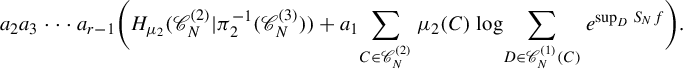 $$ \begin{align} a_2a_3 \cdots a_{r-1} \bigg( H_{\mu_2}(\mathscr{C}^{(2)}_N | \pi_2^{-1}(\mathscr{C}^{(3)}_N) ) + a_1 \!\sum_{C \in \mathscr{C}^{(2)}_N} \mu_2(C) \log{ \!\sum_{D \in \mathscr{C}^{(1)}_N(C)} e^{\sup_DS_Nf}} \bigg). \end{align} $$
This can be evaluated similarly using Lemma 3.4 as
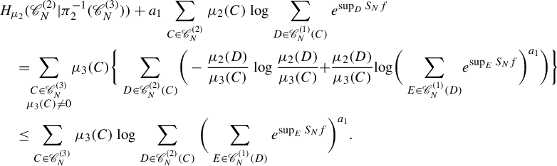 $$ \begin{align*} & H_{\mu_2}(\mathscr{C}^{(2)}_N | \pi_2^{-1}(\mathscr{C}^{(3)}_N) ) + a_1 \sum_{C \in \mathscr{C}^{(2)}_N} \mu_2(C) \log{ \sum_{D \in \mathscr{C}^{(1)}_N(C)} e^{\sup_DS_Nf}} \\ &\quad =\!\!\sum_{\substack{C \in \mathscr{C}^{(3)}_N \\ \mu_3(C) \ne 0}} \!\mu_3(C) \bigg\{ \sum_{D \in \mathscr{C}^{(2)}_N(C)}\! \bigg( -\frac{\mu_2(D)}{\mu_3(C)}\log{\frac{\mu_2(D)}{\mu_3(C)}}\! + \! \frac{\mu_2(D)}{\mu_3(C)} \!\log\!{ \bigg( \sum_{E \in \mathscr{C}^{(1)}_N(D)}\! e^{\sup_ES_Nf} \bigg)^{a_1} } \bigg) \bigg\} \\ &\quad \leq \sum_{C \in \mathscr{C}^{(3)}_N} \mu_3(C) \log{ \sum_{D \in \mathscr{C}^{(2)}_N(C)}\bigg( \sum_{E \in \mathscr{C}^{(1)}_N(D)} e^{\sup_ES_Nf} \bigg)^{a_1}}. \end{align*} $$
Continue likewise and obtain the following upper bound for equation (5.2):
 $$ \begin{align} \log{ \sum_{C^{(r)} \in \mathscr{C}^{(r)}_N} \bigg( \sum_{C^{(r-1)} \in \mathscr{C}^{(r-1)}_N(C^{(r)})} \bigg( \cdots \bigg( \sum_{C^{(1)} \in \mathscr{C}^{(1)}_N(C^{(2)})} e^{\sup_{C^{(1)}}S_Nf} \bigg)^{a_1} \cdots \bigg)^{a_{r-2}}\bigg)^{a_{r-1}}}. \end{align} $$
For
 $1\leq i \leq r$
, let
$1\leq i \leq r$
, let
 $\mathscr {C}^{(i)}_c = \{ C \in \mathscr {C}^{(i)} | C \text { is compact} \}$
. There is a positive number
$\mathscr {C}^{(i)}_c = \{ C \in \mathscr {C}^{(i)} | C \text { is compact} \}$
. There is a positive number
 $\varepsilon _i$
such that
$\varepsilon _i$
such that
 $d^{(i)}(y_1, y_2)> \varepsilon _i$
for any
$d^{(i)}(y_1, y_2)> \varepsilon _i$
for any
 $C_1, C_2 \in \mathscr {C}^{(i)}_c$
and
$C_1, C_2 \in \mathscr {C}^{(i)}_c$
and
 $y_1 \in C_1, y_2 \in C_2$
. Fix a positive number
$y_1 \in C_1, y_2 \in C_2$
. Fix a positive number
 $\varepsilon $
with
$\varepsilon $
with
 $$ \begin{align} \varepsilon < \min_{1\leq i \leq r} \varepsilon_i. \end{align} $$
Let
 $\mathscr {F}^{(i)}$
be a chain of open (N,
$\mathscr {F}^{(i)}$
be a chain of open (N,
 $\varepsilon $
)-covers of
$\varepsilon $
)-covers of
 $X_i$
(see Definition 3.1). Consider
$X_i$
(see Definition 3.1). Consider
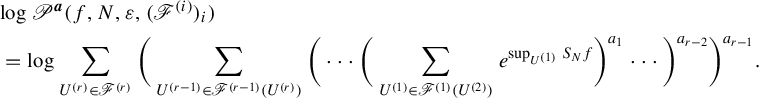 $$ \begin{align} & \log{ \mathscr{P}^{\boldsymbol{a}}( f, N, \varepsilon, (\mathscr{F}^{(i)})_i ) }\notag \\ &\ = \log{ \sum_{U^{(r)} \in \mathscr{F}^{(r)}} \bigg( \sum_{U^{(r-1)} \in \mathscr{F}^{(r-1)}(U^{(r)})} \bigg( \cdots \bigg( \sum_{U^{(1)} \in \mathscr{F}^{(1)}(U^{(2)})} e^{\sup_{U^{(1)}}S_Nf} \bigg)^{a_1} \cdots \bigg)^{a_{r-2}}\bigg)^{a_{r-1}}}. \end{align} $$
We will evaluate equation (5.4) from above by equation (5.6) up to a constant. We need the next lemma.
Lemma 5.3
-
(1) For any
$V \subset X_r$
with
$\mathrm {diam}(V,d^{(r)}_N) < \varepsilon $
,
$$ \begin{align*} | \{ D \in \mathscr{C}^{(r)}_N | D \cap V \ne \varnothing \} | \leq 2^N. \end{align*} $$
-
(2) Let
$1\leq i \leq r-1$
and
$C \in \mathscr {C}^{(i+1)}_N$
. For any
$V \subset X_i$
with
$\mathrm {diam}(V,d^{(i)}_N) < \varepsilon $
,
$$ \begin{align*} | \{ D \in \mathscr{C}^{(i)}_N(C) | D \cap V \ne \varnothing \} | \leq 2^N. \end{align*} $$


Proof. (1)
 $D \in \mathscr {C}^{(r)}_N$
can be expressed using
$D \in \mathscr {C}^{(r)}_N$
can be expressed using
 $C^{(r)}_{k_s} \in \mathscr {C}^{(r)}$
(
$C^{(r)}_{k_s} \in \mathscr {C}^{(r)}$
(
 $s =0, 1, \ldots , N-1$
) as
$s =0, 1, \ldots , N-1$
) as
 $$ \begin{align*} D = C^{(r)}_{k_0^{}} \cap T_r^{-1} C^{(r)}_{k_1^{}} \cap T_r^{-2} C^{(r)}_{k_2^{}} \cap \cdots \cap T_r^{-N+1} C^{(r)}_{k_{N-1}^{}}. \end{align*} $$
If
 $D \cap V \ne \varnothing $
, we have
$D \cap V \ne \varnothing $
, we have
 $T_r^{-s}(C^{(r)}_{k_s}) \cap V \ne \varnothing $
for every
$T_r^{-s}(C^{(r)}_{k_s}) \cap V \ne \varnothing $
for every
 $0 \leq s \leq N-1$
. Then for each s,
$0 \leq s \leq N-1$
. Then for each s,
 $$ \begin{align*} \varnothing \ne T_r^s\bigg( T_r^{-s}(C^{(r)}_{k_s}) \cap V \bigg) \subset C^{(r)}_{k_s} \cap T_r^s(V). \end{align*} $$
By equation (5.5), each
 $k_s$
is either
$k_s$
is either
 $0$
or one of the elements in
$0$
or one of the elements in
 $\{ 1, 2, \ldots , m_r \}$
. Therefore, there are at most
$\{ 1, 2, \ldots , m_r \}$
. Therefore, there are at most
 $2^N$
such sets.
$2^N$
such sets.
(2) The proof works in the same way as in item (1). C can be written using
 $J_k \in \Lambda _{i+1}^0$
(
$J_k \in \Lambda _{i+1}^0$
(
 $k=0, 1, \ldots , N-1$
) as
$k=0, 1, \ldots , N-1$
) as
 $$ \begin{align*} C = C^{(i+1)}_{J_0} \cap T_{i+1}^{-1} C^{(i+1)}_{J_1} \cap T_{i+1}^{-2} C^{(i+1)}_{J_2} \cap \cdots \cap T_{i+1}^{-N+1} C^{(i+1)}_{J_{N-1}}. \end{align*} $$
Then any
 $D \in \mathscr {C}^{(i)}_N(C)$
is of the form
$D \in \mathscr {C}^{(i)}_N(C)$
is of the form
 $$ \begin{align*} D = C^{(i)}_{J_0k_0} \cap T_i^{-1}C^{(i)}_{J_1k_1} \cap T_i^{-2}C^{(i)}_{J_2k_2} \cap \cdots \cap T_i^{-N+1}C^{(i)}_{J_{N-1}k_{N-1}} \end{align*} $$
with
 $0 \leq k_l \leq m_i$
(
$0 \leq k_l \leq m_i$
(
 $l = 1, 2, \ldots , N-1$
). If
$l = 1, 2, \ldots , N-1$
). If
 $D \cap V \ne \varnothing $
, then each
$D \cap V \ne \varnothing $
, then each
 $k_l$
is either
$k_l$
is either
 $0$
or one of the elements in
$0$
or one of the elements in
 $\{ 1, 2, \ldots , m_i \}$
. Therefore, there are at most
$\{ 1, 2, \ldots , m_i \}$
. Therefore, there are at most
 $2^N$
such sets.
$2^N$
such sets.
For any
 $C^{(1)} \in \mathscr {C}^{(1)}_N$
, there is
$C^{(1)} \in \mathscr {C}^{(1)}_N$
, there is
 $V \in \mathscr {F}^{(1)}$
with
$V \in \mathscr {F}^{(1)}$
with
 $V \cap C^{(1)} \ne \varnothing $
and
$V \cap C^{(1)} \ne \varnothing $
and
 $$ \begin{align*} e^{\sup_{C^{(1)}}S_ Nf} \leq e^{\sup_V S_N f}. \end{align*} $$
Let
 $C^{(2)} \in \mathscr {C}^{(2)}_N$
, then by Lemma 5.3,
$C^{(2)} \in \mathscr {C}^{(2)}_N$
, then by Lemma 5.3,
 $$ \begin{align*} \sum_{C^{(1)} \in \mathscr{C}^{(1)}_N(C^{(2)})} e^{\sup_{C^{(1)}}S_ Nf} \leq \sum_{\substack{U \in \mathscr{F}^{(2)} \\ U \cap C^{(2)} \ne \varnothing}} 2^N \sum_{V \in \mathscr{F}^{(1)}(U)} e^{\sup_V S_N f}. \end{align*} $$
By Lemma 3.4,
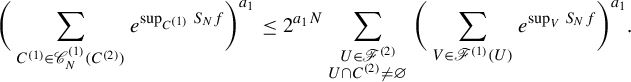 $$ \begin{align*} \bigg( \sum_{C^{(1)} \in \mathscr{C}^{(1)}_N(C^{(2)})} e^{\sup_{C^{(1)}}S_ Nf} \bigg)^{a_1} \leq 2^{a_1N} \sum_{\substack{U \in \mathscr{F}^{(2)} \\ U \cap C^{(2)} \ne \varnothing}} \bigg( \sum_{V \in \mathscr{F}^{(1)}(U)} e^{\sup_V S_N f} \bigg)^{a_1}. \end{align*} $$
For
 $C^{(3)} \in \mathscr {C}^{(3)}_N$
, we apply Lemmas 5.3 and 3.4 similarly and obtain
$C^{(3)} \in \mathscr {C}^{(3)}_N$
, we apply Lemmas 5.3 and 3.4 similarly and obtain
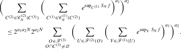 $$ \begin{align*} &\bigg( \sum_{C^{(2)} \in \mathscr{C}^{(2)}_N(C^{(3)})} \bigg( \sum_{C^{(1)} \in \mathscr{C}^{(1)}_N(C^{(2)})} e^{\sup_{C^{(1)}}S_ Nf} \bigg)^{a_1} \bigg)^{a_2} \\ &\quad \leq 2^{a_1a_2N} 2^{a_2N} \sum_{\substack{O \in \mathscr{F}^{(3)} \\ O \cap C^{(3)} \ne \varnothing}} \bigg( \sum_{U \in \mathscr{F}^{(2)}(O)} \bigg( \sum_{V \in \mathscr{F}^{(1)}(U)} e^{\sup_V S_N f} \bigg)^{a_1} \bigg)^{a_2}. \end{align*} $$
We continue this reasoning and get
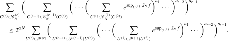 $$ \begin{align*} &\!\kern0.1pt\!\sum_{C^{(r)} \in \mathscr{C}^{(r)}_N} \bigg( \sum_{C^{(r-1)} \in \mathscr{C}^{(r-1)}_N(C^{(r)})} \bigg( \cdots \bigg( \sum_{C^{(1)} \in \mathscr{C}^{(1)}_N(C^{(2)})} e^{\sup_{C^{(1)}}S_Nf} \bigg)^{a_1} \cdots \bigg)^{a_{r-2}}\bigg)^{a_{r-1}} \\& \quad \leq 2^{\alpha N}\! \sum_{U^{(r)} \in \mathscr{F}^{(r)}} \!\bigg( \sum_{U^{(r-1)} \in \mathscr{F}^{(r-1)}(U^{(r)})} \bigg( \cdots \bigg( \sum_{U^{(1)} \in \mathscr{F}^{(1)}(U^{(2)})} e^{\sup_{U^{(1)}}S_Nf} \bigg)^{a_1} \cdots \bigg)^{a_{r-2}}\bigg)^{a_{r-1}}. \end{align*} $$
Here,
 $\alpha $
stands for
$\alpha $
stands for
 $\sum _{i=1}^{r-1} a_i a_{i+1}\cdots a_{r-1}$
. We take the logarithm of both sides; the left-hand side equals equation (5.4), which is an upper bound for equation (5.2). Furthermore, consider the infimum over the chain of open (N,
$\sum _{i=1}^{r-1} a_i a_{i+1}\cdots a_{r-1}$
. We take the logarithm of both sides; the left-hand side equals equation (5.4), which is an upper bound for equation (5.2). Furthermore, consider the infimum over the chain of open (N,
 $\varepsilon $
)-covers
$\varepsilon $
)-covers
 $(\mathscr {F}^{(i)})_i$
on the right-hand side. By Remark 3.2, this yields
$(\mathscr {F}^{(i)})_i$
on the right-hand side. By Remark 3.2, this yields
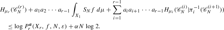 $$ \begin{align*} &H_{\mu_r}(\mathscr{C}^{(r)}_N) + a_1a_2 \cdots a_{r-1} \int_{X_1} S_Nf\,d\mu + \sum_{i=1}^{r-1} a_i a_{i+1} \cdots a_{r-1} H_{\mu_i}(\mathscr{C}^{(i)}_N | \pi_i^{-1}(\mathscr{C}^{(i+1)}_N) ) \\ &\quad \leq \log{P^{\boldsymbol{a}}_r(X_r, f, N, \varepsilon)} + \alpha N \log{2}. \\ \end{align*} $$
Divide by N, then let
 $N \to \infty $
and
$N \to \infty $
and
 $\varepsilon \to 0$
. We obtain
$\varepsilon \to 0$
. We obtain
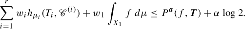 $$ \begin{align*} \sum_{i=1}^r w_i h_{\mu_i}(T_i, \mathscr{C}^{(i)}) + w_1 \int_{X_1} f\,d\mu \leq P^{\boldsymbol{a}}(f, \boldsymbol{T}) + \alpha \log{2}. \end{align*} $$
Lemma 5.2 yields
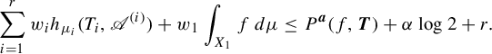 $$ \begin{align*} \sum_{i=1}^r w_i h_{\mu_i}(T_i, \mathscr{A}^{(i)}) + w_1 \int_{X_1} f\,d\mu \leq P^{\boldsymbol{a}}(f, \boldsymbol{T}) + \alpha \log{2} + r. \end{align*} $$
We take the supremum over the partitions
 $(\mathscr {A}^{(i)})_i$
:
$(\mathscr {A}^{(i)})_i$
:
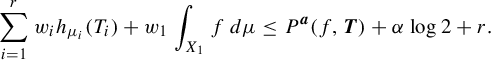 $$ \begin{align*} \sum_{i=1}^r w_i h_{\mu_i}(T_i) + w_1 \int_{X_1} f\,d\mu \leq P^{\boldsymbol{a}}(f, \boldsymbol{T}) + \alpha \log{2} + r. \end{align*} $$
By the argument at the beginning of this proof, we conclude that
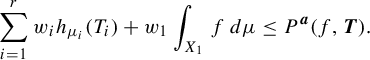 $$ \begin{align*} \sum_{i=1}^r w_i h_{\mu_i}(T_i) + w_1 \int_{X_1} f\,d\mu \leq P^{\boldsymbol{a}}(f, \boldsymbol{T}).\\[-42pt] \end{align*} $$
6. Example: sofic sets
Kenyon and Peres [Reference Kenyon and PeresKP96-2] calculated the Hausdorff dimension of sofic sets in
 $\mathbb {T}^2$
. In this section, we will see that we can calculate the Hausdorff dimension of certain sofic sets in
$\mathbb {T}^2$
. In this section, we will see that we can calculate the Hausdorff dimension of certain sofic sets in
 $\mathbb {T}^d$
with arbitrary d. We give an example for the case
$\mathbb {T}^d$
with arbitrary d. We give an example for the case
 $d=3$
.
$d=3$
.
6.1. Definition of sofic sets
This subsection is referred to [Reference Kenyon and PeresKP96-2]. Weiss [Reference WeissWe82] defined sofic systems as subshifts which are factors of shifts of finite type. Boyle, Kitchens, and Marcus proved in [Reference Boyle, Kitchens and MarcusBKM85] that this is equivalent to the following definition.
Definition 6.1. [Reference Kenyon and PeresKP96-2, Proposition 3.6]
Consider a finite directed graph
 $G = \langle V, E \rangle $
in which loops and multiple edges are allowed. Suppose its edges are colored in l colors in a ‘right-resolving’ fashion: every two edges emanating from the same vertex have different colors. Then the set of color sequences that arise from infinite paths in G is called the sofic system.
$G = \langle V, E \rangle $
in which loops and multiple edges are allowed. Suppose its edges are colored in l colors in a ‘right-resolving’ fashion: every two edges emanating from the same vertex have different colors. Then the set of color sequences that arise from infinite paths in G is called the sofic system.
Let
 $m_1 \leq m_2 \leq \cdots \leq m_r$
be natural numbers, T an endomorphism on
$m_1 \leq m_2 \leq \cdots \leq m_r$
be natural numbers, T an endomorphism on
 $\mathbb {T}^r = \mathbb {R}^r/\mathbb {Z}^r$
represented by the diagonal matrix
$\mathbb {T}^r = \mathbb {R}^r/\mathbb {Z}^r$
represented by the diagonal matrix
 $A = \mathrm {diag}(m_1, m_2, \ldots , m_r)$
, and
$A = \mathrm {diag}(m_1, m_2, \ldots , m_r)$
, and
 $D = \prod _{i=1}^r \{0, 1, \ldots , m_i-1\}$
. Define a map
$D = \prod _{i=1}^r \{0, 1, \ldots , m_i-1\}$
. Define a map
 $R_r: D^{\mathbb {N}} \rightarrow \mathbb {T}^r$
by
$R_r: D^{\mathbb {N}} \rightarrow \mathbb {T}^r$
by
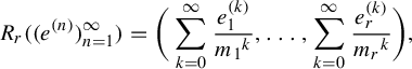 $$ \begin{align*} R_r((e^{(n)})_{n=1}^{\infty}) = \bigg( \sum_{k=0}^{\infty} \frac{e^{(k)}_1}{{m_1}^k}, \ldots, \sum_{k=0}^{\infty} \frac{e^{(k)}_r}{{m_r}^k} \bigg), \end{align*} $$
where
 $e^{(k)} = (e^{(k)}_1, \ldots , e^{(k)}_r) \in D$
for each k. Suppose the edges in some finite directed graph are labeled by the elements in D in the right-resolving fashion, and let
$e^{(k)} = (e^{(k)}_1, \ldots , e^{(k)}_r) \in D$
for each k. Suppose the edges in some finite directed graph are labeled by the elements in D in the right-resolving fashion, and let
 $S \subset D^{\mathbb {N}}$
be the resulting sofic system. The image of S under
$S \subset D^{\mathbb {N}}$
be the resulting sofic system. The image of S under
 $R_r$
is called a sofic set.
$R_r$
is called a sofic set.
6.2. An example of a sofic set
Here we will look at an example of a sofic set and calculate its Hausdorff dimension via its weighted topological entropy. Let
 $D = \{0, 1\} \times \{0, 1, 2\} \times \{0, 1, 2, 3\}$
, and consider the directed graph
$D = \{0, 1\} \times \{0, 1, 2\} \times \{0, 1, 2, 3\}$
, and consider the directed graph
 $G = \langle V, E \rangle $
with
$G = \langle V, E \rangle $
with
 $V = \{1, 2, 3\}$
and D-labeled edges E in Figure 2.
$V = \{1, 2, 3\}$
and D-labeled edges E in Figure 2.
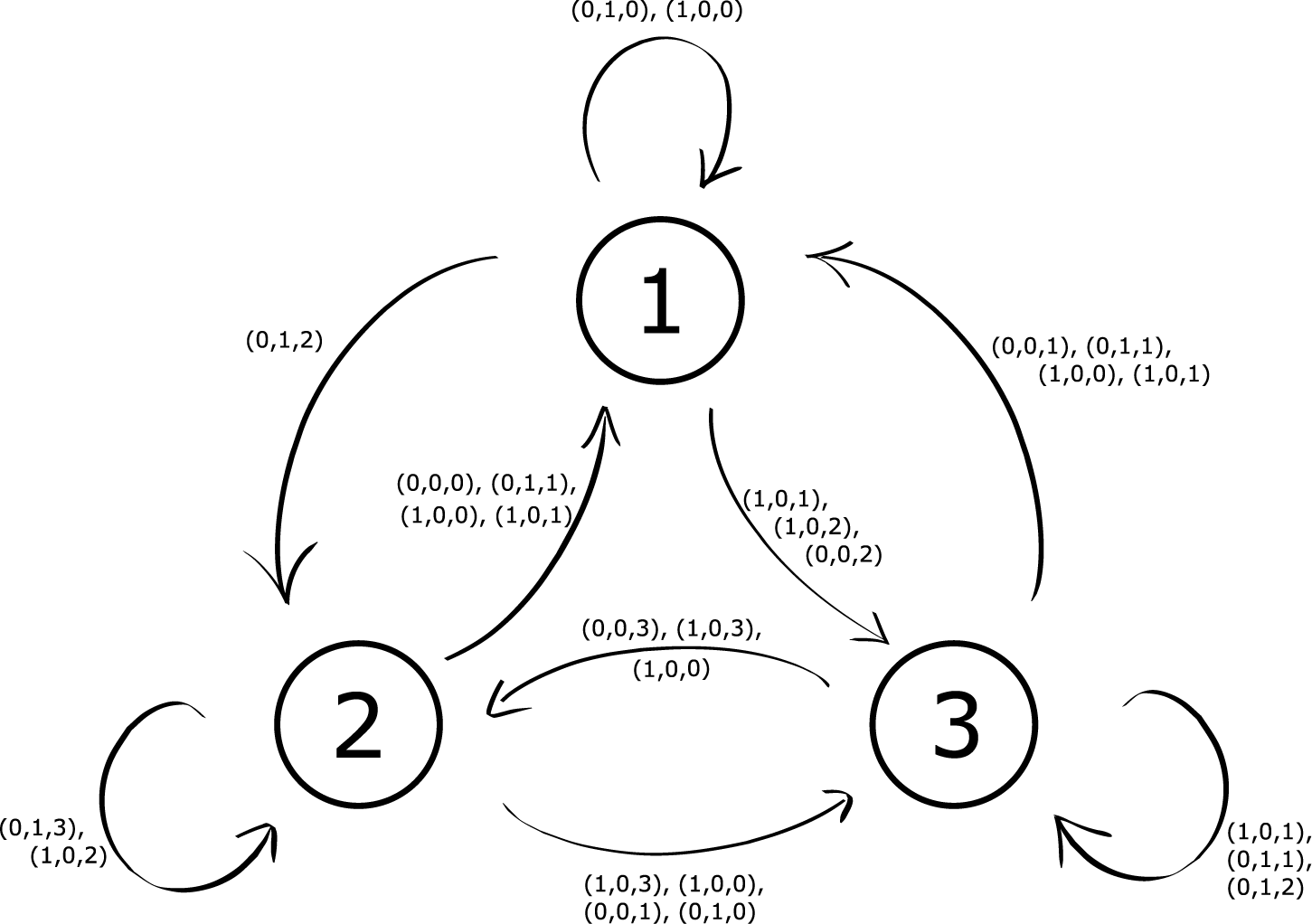
Figure 2 Directed graph G.
Let
 $Y_1 \subset D^{\mathbb {N}}$
be the resulting sofic system. Let
$Y_1 \subset D^{\mathbb {N}}$
be the resulting sofic system. Let
 $C = \{0, 1\} \times \{0, 1, 2\}$
and
$C = \{0, 1\} \times \{0, 1, 2\}$
and
 $B = \{0, 1\}$
. Define
$B = \{0, 1\}$
. Define
 $p_1: D \rightarrow C$
and
$p_1: D \rightarrow C$
and
 $p_2: C \rightarrow B$
by
$p_2: C \rightarrow B$
by
 $$ \begin{align*} p_1(i, j, k) = (i, j), \quad p_2(i, j) = i. \end{align*} $$
Let
 $p_1^{\mathbb {N}}: D^{\mathbb {N}} \rightarrow C^{\mathbb {N}}$
and
$p_1^{\mathbb {N}}: D^{\mathbb {N}} \rightarrow C^{\mathbb {N}}$
and
 $p_2^{\mathbb {N}}: C^{\mathbb {N}} \rightarrow B^{\mathbb {N}}$
be the product map of
$p_2^{\mathbb {N}}: C^{\mathbb {N}} \rightarrow B^{\mathbb {N}}$
be the product map of
 $p_1$
and
$p_1$
and
 $p_2$
, respectively. Set
$p_2$
, respectively. Set
 $Y_2 = p_1^{\mathbb {N}}(Y_1)$
and
$Y_2 = p_1^{\mathbb {N}}(Y_1)$
and
 $Y_3 = p_2^{\mathbb {N}}(Y_2)$
. Note that
$Y_3 = p_2^{\mathbb {N}}(Y_2)$
. Note that
 $Y_2 = \{ (0, 0), (1,0), (0, 1) \}^{\mathbb {N}}$
and
$Y_2 = \{ (0, 0), (1,0), (0, 1) \}^{\mathbb {N}}$
and
 $Y_3 = \{0, 1\}^{\mathbb {N}}$
, meaning they are full shifts.
$Y_3 = \{0, 1\}^{\mathbb {N}}$
, meaning they are full shifts.
The sets
 $X_i = R_i(Y_i) (i = 1, 2, 3)$
are sofic sets. Define
$X_i = R_i(Y_i) (i = 1, 2, 3)$
are sofic sets. Define
 $\pi _1: X_1 \rightarrow X_2$
and
$\pi _1: X_1 \rightarrow X_2$
and
 $\pi _2: X_2 \rightarrow X_3$
by
$\pi _2: X_2 \rightarrow X_3$
by
 $$ \begin{align*} \pi_1(x, y, z) = (x, y), \quad \pi_2(x, y) = x. \end{align*} $$
Furthermore, let
 $T_1$
,
$T_1$
,
 $T_2$
, and
$T_2$
, and
 $T_3$
be the endomorphism on
$T_3$
be the endomorphism on
 $X_1$
,
$X_1$
,
 $X_2$
, and
$X_2$
, and
 $X_3$
represented by the matrices
$X_3$
represented by the matrices
 $\mathrm {diag}(2, 3, 4)$
,
$\mathrm {diag}(2, 3, 4)$
,
 $\mathrm {diag}(2, 3)$
, and
$\mathrm {diag}(2, 3)$
, and
 $\mathrm {diag}(2)$
, respectively. Then
$\mathrm {diag}(2)$
, respectively. Then
 $(X_i, T_i)_i$
and
$(X_i, T_i)_i$
and
 $(\pi _i)_i$
form a sequence of dynamical systems.
$(\pi _i)_i$
form a sequence of dynamical systems.
For a natural number N, denote by
 $Y_i|_N$
the restriction of
$Y_i|_N$
the restriction of
 $Y_i$
to its first N coordinates, and let
$Y_i$
to its first N coordinates, and let
 $p_{i, N}: Y_i|_N \rightarrow Y_{i+1}|_N$
be the projections for
$p_{i, N}: Y_i|_N \rightarrow Y_{i+1}|_N$
be the projections for
 $i = 1, 2$
. As in Example 1.4, we have for any exponent
$i = 1, 2$
. As in Example 1.4, we have for any exponent
 $\boldsymbol {a} = (a_1, a_2) \in [0, 1]^2$
,
$\boldsymbol {a} = (a_1, a_2) \in [0, 1]^2$
,
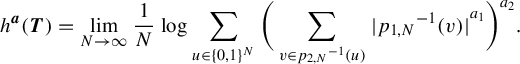 $$ \begin{align*} h^{\boldsymbol{a}}(\boldsymbol{T}) = \lim_{N \to \infty} \frac{1}{N} \log{ \sum_{u \in \{0, 1\}^N} {\bigg( \sum_{v \in {p_{2, N}}^{-1}(u)} {| {p_{1, N}}^{-1}(v) |}^{a_1} \bigg)}^{a_2}}. \end{align*} $$
Now, let us evaluate
 $| {p_{1, N}}^{-1}(v) |$
using matrix products. This idea of using matrix products is due to Kenyon and Peres [Reference Kenyon and PeresKP96-2]. Fix
$| {p_{1, N}}^{-1}(v) |$
using matrix products. This idea of using matrix products is due to Kenyon and Peres [Reference Kenyon and PeresKP96-2]. Fix
 $(a, b) \in {\{0, 1\}}^2$
and let
$(a, b) \in {\{0, 1\}}^2$
and let
 $$ \begin{align*} a_{ij} = | \{ e \in E | e \text{ is from } j \text{ to } i \text{ and the first two coordinates of its label are } (a, b) \} |. \end{align*} $$
Define a
 $3 \times 3$
matrix by
$3 \times 3$
matrix by
 $A_{(a, b)} = (a_{ij})_{ij}$
. Then we have
$A_{(a, b)} = (a_{ij})_{ij}$
. Then we have
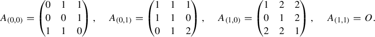 $$ \begin{align*} A_{(0, 0)} = \begin{pmatrix} 0 & 1 & 1 \\ 0 & 0 & 1 \\ 1 & 1 & 0 \\ \end{pmatrix},\quad A_{(0, 1)} = \begin{pmatrix} 1 & 1 & 1 \\ 1 & 1 & 0 \\ 0 & 1 & 2 \\ \end{pmatrix},\quad A_{(1, 0)} = \begin{pmatrix} 1 & 2 & 2 \\ 0 & 1 & 2 \\ 2 & 2 & 1 \\ \end{pmatrix},\quad A_{(1, 1)} = O. \end{align*} $$
Note that
 ${A_{(0, 0)}}^2 = A_{(0, 1)}$
and
${A_{(0, 0)}}^2 = A_{(0, 1)}$
and
 ${A_{(0, 0)}}^3 = A_{(1, 0)}$
. For
${A_{(0, 0)}}^3 = A_{(1, 0)}$
. For
 $v = (v_1, \ldots , v_N) \in Y_2|_N$
, we have
$v = (v_1, \ldots , v_N) \in Y_2|_N$
, we have
 $$ \begin{align*} | {p_{1, N}}^{-1}(v) | \asymp \| A_{v_1} A_{v_2} \cdots A_{v_N} \|. \end{align*} $$
Here,
 $A \asymp B $
means there is a constant
$A \asymp B $
means there is a constant
 $c> 0$
independent of N with
$c> 0$
independent of N with
 $c^{-1}B \leq A \leq cB$
. For
$c^{-1}B \leq A \leq cB$
. For
 $\alpha = ({1 + \sqrt {5}})/{2}$
, we have
$\alpha = ({1 + \sqrt {5}})/{2}$
, we have
 $\alpha ^2 = \alpha + 1$
and
$\alpha ^2 = \alpha + 1$
and
 $$ \begin{align*} A_{(0, 0)} \begin{pmatrix} \alpha \\ 1 \\ \alpha \\ \end{pmatrix} = \begin{pmatrix} 1 + \alpha \\ \alpha \\ 1 + \alpha \\ \end{pmatrix} = \alpha \begin{pmatrix} \alpha \\ 1 \\ \alpha \\ \end{pmatrix}\!, \quad A_{(0, 1)} \begin{pmatrix} \alpha \\ 1 \\ \alpha \\ \end{pmatrix} = \alpha^2 \begin{pmatrix} \alpha \\ 1 \\ \alpha \\ \end{pmatrix}\!, \quad A_{(1, 0)} \begin{pmatrix} \alpha \\ 1 \\ \alpha \\ \end{pmatrix} = \alpha^3 \begin{pmatrix} \alpha \\ 1 \\ \alpha \\ \end{pmatrix}\!. \end{align*} $$
Therefore,
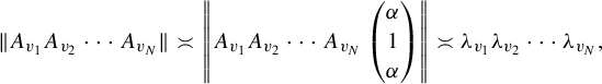
where
 $\unicode{x3bb} _{(0,0)} = \alpha $
,
$\unicode{x3bb} _{(0,0)} = \alpha $
,
 $\unicode{x3bb} _{(0,1)} = \alpha ^2$
,
$\unicode{x3bb} _{(0,1)} = \alpha ^2$
,
 $\unicode{x3bb} _{(1,0)} = \alpha ^3$
.
$\unicode{x3bb} _{(1,0)} = \alpha ^3$
.
Take
 $u \in Y_3 = {\{0, 1\}}^{\mathbb {N}}$
and suppose there are n numbers of zeros in u. Also, if there are k numbers of
$u \in Y_3 = {\{0, 1\}}^{\mathbb {N}}$
and suppose there are n numbers of zeros in u. Also, if there are k numbers of
 $(0, 0)$
terms in
$(0, 0)$
terms in
 $v = (v_1, \ldots , v_N) \in {p_{2, N}}^{-1}(u)$
, there are
$v = (v_1, \ldots , v_N) \in {p_{2, N}}^{-1}(u)$
, there are
 $n - k$
numbers of
$n - k$
numbers of
 $(0, 1)$
terms and
$(0, 1)$
terms and
 $N - n$
numbers of
$N - n$
numbers of
 $(1, 0)$
terms in v. Then,
$(1, 0)$
terms in v. Then,
Therefore (recall that
 $Y_2 = \{(0,0), (1,0), (0,1)\}^{\mathbb {N}}$
),
$Y_2 = \{(0,0), (1,0), (0,1)\}^{\mathbb {N}}$
),
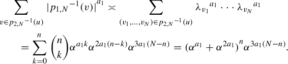
This implies
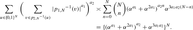 $$ \begin{align*} \sum_{u \in \{0, 1\}^N} {\bigg( \sum_{v \in {p_{2, N}}^{-1}(u)} {| {p_{1, N}}^{-1}(v) |}^{a_1} \bigg)}^{a_2} &\asymp \sum_{n=0}^N {N \choose n}{( \alpha^{a_1} + \alpha^{2a_1})}^{a_2n} \alpha^{3a_1a_2(N-n)} \\ &= \{ {( \alpha^{a_1} + \alpha^{2a_1} )}^{a_2} + \alpha^{3a_1a_2}\}^N. \end{align*} $$
We conclude that
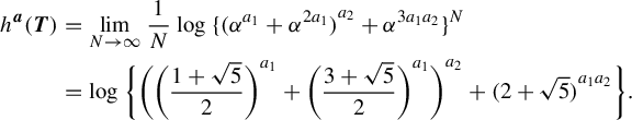 $$ \begin{align*} h^{\boldsymbol{a}}(\boldsymbol{T}) &= \lim_{N \to \infty} \frac{1}{N} \log{\{ {( \alpha^{a_1} + \alpha^{2a_1} )}^{a_2} + \alpha^{3a_1a_2} \}^N} \\ &= \log{ \bigg\{ {\bigg( {\bigg( \frac{1 + \sqrt{5}}{2} \bigg)}^{a_1} + {\bigg( \frac{3 + \sqrt{5}}{2} \bigg)}^{a_1} \bigg)}^{a_2} + {(2+\sqrt{5})}^{a_1a_2} \bigg\}}. \end{align*} $$
As in Example 1.4, the Hausdorff dimension of
 $X_1$
is obtained by letting
$X_1$
is obtained by letting
 $a_1 = \log _4{3}$
and
$a_1 = \log _4{3}$
and
 $a_2 = \log _3{2}$
:
$a_2 = \log _3{2}$
:
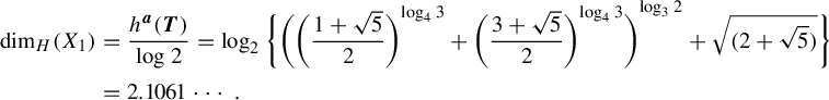 $$ \begin{align*} \mathrm{dim}_H(X_1) &= \frac{h^{\boldsymbol{a}}(\boldsymbol{T})}{\log{2}} = \log_2{ \bigg\{ {\bigg( {\bigg( \frac{1 + \sqrt{5}}{2} \bigg)}^{\log_4{3}} + {\bigg( \frac{3 + \sqrt{5}}{2} \bigg)}^{\log_4{3}} \bigg)}^{\log_3{2}} + \sqrt{{(2+\sqrt{5})}} \bigg\}} \\ &= 2.1061\cdots. \end{align*} $$
Acknowledgements
I am deeply grateful to my mentor, Masaki Tsukamoto, who not only has reviewed this paper several times throughout the writing process but has patiently helped me understand ergodic theory in general with his expertise. I also want to thank my family and friends for their unconditional support and everyone who has participated in my study for their time and willingness to share their knowledge. This work could not have been possible without their help.


