2. Simulations and data summary

This work utilizes an LES of a frontal spin down under uniform wind stress and without waves (or Stokes drift) as described in Reference Hamlington, Van Roekel, Fox-Kemper, Julien and ChiniHamlington et al. (2014). Other studies have revisited passive tracers mimicking biological tracer transport (Reference Smith, Hamlington and Fox-KemperSmith, Hamlington & Fox-Kemper 2016), frontogenesis (Reference Suzuki and Fox-KemperSuzuki & Fox-Kemper 2016) and PV spectra (Reference Bodner and Fox-KemperBodner & Fox-Kemper 2020) in these runs; this analysis focuses on the standard diagnostic practices distinguishing turbulent ‘mixing’ from submesoscale ‘overturning’ underpinning parametrizations affecting buoyancy, energy and PV.

The horizontal doubly periodic domain is $20\,{\rm km}\times 20\,{\rm km}$ with 4.9 m resolution, and the vertical extent in 160 m with 1.25 m resolution. The simulation contains a warm filament with a uniform surface wind stress of $\tau = 0.025\,{\rm N}\,{\rm m}^{-2}$ aligned at a $30^{\circ }$ angle from the geostrophic flow. The analysis includes data from days 10 and 11 of the simulation. It is convenient to divide the simulation spatially into three regions: (1) NOFRONT, (2) STABLE and (3) UNSTABLE (figure 1). The NOFRONT region represents the neutral boundary layer, where turbulent motions are driven by surface wind stress and deliver modest entrainment. In the STABLE region, the constant and uniform, partly upfront, wind stress induces an Ekman transport to the right of the wind direction. This Ekman flow transports warm water over the cold side of the front (upfront wind/stable), thereby stratifying the boundary layer. In the UNSTABLE region, Ekman flow transports cold water over the warm side of the front, causing boundary layer convection from the Ekman buoyancy flux (i.e. downfront winds; Reference Thomas and LeeThomas & Lee 2005). This front develops unstable baroclinic instabilities that drive restratifying circulations within the boundary layer. The simulations were designed such that eddy restratification in this UNSTABLE region ($Q \sim 25\,{\rm W}\,{\rm m}^{-2}$) is larger than Ekman-driven convection ($Q \sim -13\,{\rm W}\,{\rm m}^{-2}$) and similar in magnitude to the vertical heat flux in the NOFRONT region from shear-driven mixing and entrainment ($Q\sim -10\,{\rm W}\,{\rm m}^{-2}$). Due to the finite-amplitude baroclinic waves, the Ekman-induced boundary layer convection impacts 20 % of the UNSTABLE region. Realistic forcing conditions might strengthen any one mechanism to dominate over the others (Reference Haney, Bachman, Cooper, Kupper, McCaffrey, Van Roekel, Stevenson, Fox-Kemper and FerrariHaney et al. 2012). Note that the UNSTABLE region may also possess forced symmetric instabilities (Reference Bachman, Fox-Kemper, Taylor and ThomasBachman et al. 2017). For the time window of data analysed, the STABLE and UNSTABLE regions are more stratified than the NOFRONT region, because of Ekman and mixed-layer instability restratification, respectively. On average, mixed-layer depths are about 50, 45 and 40 m for the NOFRONT, UNSTABLE and STABLE regions, respectively. The fully developed eddy field and restratifying front at day 10 can be seen in figure 1.

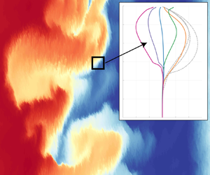
Figure 1. Surface temperature at day 10 of the H14 runs. (a) The entire model domain is separated into regimes: homogeneous turbulence region (NO FRONT, orange), front with stabilizing winds (STABLE, green), front with unstable winds and baroclinic instability (UNSTABLE,blue). (b) A $2\,{km}\times 2\,{km}$ close-up of the UNSTABLE region. The dashed area is a $400\,{m}\times 400\,{m}$ box, where 400 m length scale is the transition between quasi-2-D and 3-D flows (see H14). The colourbar is the same for both panels.

Fluid motions in each of these domains are influenced by the dynamics on all scales, with velocity spectral slopes consistent with two-dimensional (2-D) circulation involving frontal velocity jumps at larger scales ($k^{-2}$ slope), transitioning to three-dimensional (3-D) turbulence at ${\sim }400\,{\rm m}$ (Reference Hamlington, Van Roekel, Fox-Kemper, Julien and ChiniHamlington et al. 2014). Though velocity spectra support 3-D turbulence below 400 m, a detailed look at surface temperature (figure 1) reveals rich horizontal structure at the $O({\rm m})$ scale, thus challenging the assumption of horizontal homogeneity that often sets the prerequisite for OSBL turbulence physics (Reference Monin and ObukhovMonin & Obukhov 1954). The goal is to evaluate how these fine-scale flows compare with buoyancy fluxes approximated by current OSBL parametrizations. To do this, three different OSBL parametrizations are implemented using the General Ocean Turbulence Modelling (GOTM; Reference Burchard, Bolding and VillarrealBurchard, Bolding & Villarreal 1999) framework (hereafter referred to as one-dimensional (1-D)) as summarized in table 1.

Table 1. List of parametrizations used in this study.

The ingredients of extant submesoscale parametrizations (Reference Fox-Kemper, Ferrari and HallbergFox-Kemper et al. 2008; Reference Bachman, Fox-Kemper, Taylor and ThomasBachman et al. 2017) are diagnosed by scale separation.

3. Separation of scales

Turbulent flows are often expressed in terms of their statistical mean through the Reynolds-averaged equations, whereby instantaneous values are represented as the sum of an average value (in space or time) and fluctuations from the mean. The interpretation of the turbulence then is subject to the resolution of the fluctuations and definition of the mean fields. Here, a multi-level Reynolds decomposition is utilized to separate submesoscale turbulence from fine-scale turbulence. The first decomposition for any variable $c$ is ${c} = \tilde {c} + c'$, where $\tilde {c}$ represents a square boxcar average over a to-be-determined length scale to be permitted as submesoscale, and $c'$ are the finer-than-submesoscale fluctuations from that mean. The submesoscale can also be averaged further along the front indicated by an overbar, $\bar {c}$. Thus, $\tilde {c} = {c^a} + c^{s}$, where ${c^a}$ is the domain average of $\tilde {c}$ in the along-front direction (hereafter referred to as along-front average). Here $c^{s}$ are the submesoscale fluctuations from the along-front mean. Combined, the decomposition becomes

(3.1a–c)\begin{equation} c = \tilde{c} + c' = c^a + c^s + c',\quad \tilde{c} = c^a + c^s,\quad \overline{\tilde{c}} = c^a. \end{equation}

Note that $c'$ is not the fluctuation term in a traditional along-front Reynolds decomposition, $c - \bar {c} \ne c'$; rather, it is the fluctuation from a submesoscale-permitting resolution as in (3.1a–c) – similar to the role that a boundary layer mixing parametrization would play in a submesoscale-permitting model (e.g. Reference Gula, Molemaker and McWilliamsGula, Molemaker & McWilliams 2014; Reference Su, Wang, Klein, Thompson and MenemenlisSu et al. 2018). On the other hand, the submesoscale-permitting mean, $\tilde {c}$, may be analogous to a coarse resolution regional or process model that resolves submesoscale turbulence but not fine-scale motions, which is parametrized. Making this scale separation specific then rests on the definition of the minimum submesoscale length permitted in $\tilde {c}$. A sensible definition is the transition scale from 2-D to 3-D turbulence scaling. Our choice is 396.9 m to accommodate grid resolution and is based on the 400 m flow transition for this simulation described in Reference Hamlington, Van Roekel, Fox-Kemper, Julien and ChiniHamlington et al. (2014) (horizontal kinetic energy spectral slope) and Reference Bodner and Fox-KemperBodner & Fox-Kemper (2020) (PV spectral slope).

The along-front and submesoscale means are both linear operators, and they are furthermore idempotent Reynolds averages, which distinguishes them from more generic ‘linear filters’ more commonly used in LES (e.g. Reference Fox-Kemper and MenemenlisFox-Kemper & Menemenlis 2008; Reference Storer, Buzzicotti, Khatri, Griffies and AluieStorer et al. 2022). Differentiation and integration are also linear operators, but they do not commute with averaging generally. A further discussion of the specific operators used, their limitations and estimates of error resulting from these choices is in Appendix A.

The multi-level Reynolds decomposition for a Boussinesq fluid is thus

(3.2)\begin{equation} \frac{\partial }{\partial t}(b^a + b^s + b') = {-}\frac{\partial}{\partial x_j}[(u_j^a + u_j^s + u'_j)(b^a + b^s + b')] -\mathcal{V}_{ij}^{b}, \end{equation}

(3.3)\begin{align} \frac{\partial }{\partial t}(u_i^a + u_i^s + u'_i) & = {-}\frac{\partial}{\partial x_j}[(u_j^a + u_j^s + u'_j) (u_i^a + u_i^s + u'_i)] -\frac{1}{\rho_o}\frac{\partial}{\partial x_i}(p^a + p^s + p') \nonumber\\ &\quad - 2\epsilon_{ikj}\varOmega_j(u_k^a + u_k^s + u'_k) - \mathcal{V}_{ij}^{m}. \end{align}

Here, $b$ is buoyancy, $u$ is velocity, $p$ is pressure, $\varOmega$ is planetary rotation rate and $\mathcal {V}_{ij}^{b}$ and $\mathcal {V}_{ij}^{m}$ are the divergence of the diffusive buoyancy and viscous momentum fluxes, respectively. Operating on (3.2) and (3.3), the submesoscale Reynolds average, $\widetilde {()}$, is taken first (noting that all terms linear in primes vanish), followed by the along-front average, $\overline {()}$ (noting that all terms linear in submesoscale variables vanish), yielding the multi-level Reynolds-averaged equations for along-front mean of buoyancy and momentum:

(3.4)\begin{equation} \frac{\partial b^{a}}{\partial t} = {-}\frac{\partial}{\partial x_j}[u^{a}_j b^{a}] - \frac{\partial}{\partial x_j} \overline{\widetilde{b^{s} u^{s}_j}} - \frac{\partial}{\partial x_j} \overline{\widetilde{b' u'_j}} - \overline{\widetilde{\mathcal{V}_{ij}^{b}}} \end{equation}

and

(3.5)\begin{equation} \frac{\partial u^{a}_i}{\partial t} = {-}\frac{\partial }{\partial x_j}[u^{a}_j u^{a}_i] -\frac{1}{\rho_o}\frac{\partial p^{a}}{\partial x_i} - 2\epsilon_{ikj}\varOmega_ju^{a}_k + \frac{\partial}{\partial x_j}\overline{\widetilde{u^{s}_i u^{s}_j}} - \frac{\partial}{\partial x_j} \overline{\widetilde{u'_i u'_j}} - \overline{\widetilde{\mathcal{V}_{ij}^{m}}}. \end{equation}

The covariance terms capture the transport of properties at the different scales, separating clearly the transport by submesoscale turbulence from transport due to fine-scale motions.

This Reynolds-averaging approach is more similar to the scale-separation assumption typical of ocean climate models (i.e. scale-separated Reynolds averaging) rather than cascade-filtering approaches more typical of LES studies (see e.g. Reference Fox-Kemper and MenemenlisFox-Kemper & Menemenlis 2008; Reference Aluie, Hecht and VallisAluie, Hecht & Vallis 2018). The reason for the choice of Reynolds averaging is to explore whether the approach taken in ocean climate modelling is deficient when considering the turbulence of both the submesoscale (e.g. Reference Fox-Kemper, Ferrari and HallbergFox-Kemper et al. 2008) and the fine scale (e.g. Reference Large, McWilliams and DoneyLarge et al. 1994), potentially including resolving the submesoscale but not the fine scale (e.g. Reference Gula, Molemaker and McWilliamsGula et al. 2014; Reference Su, Wang, Klein, Thompson and MenemenlisSu et al. 2018). Note that these scales are neighbouring, but with spectrally distinct slopes in this simulation and recognizable as quasi-2-D and 3-D cascades (Reference Hamlington, Van Roekel, Fox-Kemper, Julien and ChiniHamlington et al. 2014; Reference Bodner and Fox-KemperBodner & Fox-Kemper 2020). Equation (3.4) is similar to the triple decomposition used with observations to evaluate along isopycnal tracer dispersion in the North Atlantic (Reference Ferrari and PolzinFerrari & Polzin 2005; Reference Smith and FerrariSmith & Ferrari 2009) and Southern Ocean (Reference Garabato, Polzin, Ferrari, Zika and ForryanGarabato et al. 2016) stratified ocean interior, but here the decomposition is used in the context of the OSBL. This Reynolds decomposition will be used to evaluate the role of multi-scale transport in the upper ocean buoyancy budget in a form that lends itself to being compared with current subgridscale parametrizations. The Reynolds fluxes that arise from the nonlinearity of the advective term transport and stir tracers. These processes are distinct from mixing that acts to homogenize tracers. Yet delineating between the two becomes convoluted when considering how they are represented by parametrizations, each of which treats these terms differently. In this paper, the term mixing is consistent with the OSBL parametrization convention, where the stirring by boundary layer eddies is conceptualized as a mixing term.

Submesoscale motions manifest in the buoyancy and energy budgets and are linked to the fluid's PV. In terms of the buoyancy budget and energetics (Reference Fox-Kemper, Ferrari and HallbergFox-Kemper et al. 2008, Reference Fox-Kemper, Danabasoglu, Ferrari, Griffies, Hallberg, Holland, Maltrud, Peacock and Samuels2011), submesoscales impact stratification and enhance the transfer of energy towards dissipative scales (Reference Capet, McWilliams, Molemaker and ShchepetkinCapet et al. 2008; Reference Taylor and FerrariTaylor & Ferrari 2010; Reference Thomas and TaylorThomas & Taylor 2010; Reference McWilliamsMcWilliams 2016). Additionally, PV is a dynamically relevant tracer to understand and identify submesoscale processes (Reference Bodner and Fox-KemperBodner & Fox-Kemper 2020; Reference Johnson, Lee, D'Asaro, Wenegrat and ThomasJohnson et al. 2020), especially symmetric instability (Reference HoskinsHoskins 1974; Reference Thomas, Taylor, Ferrari and JoyceThomas et al. 2013; Reference Haney, Fox-Kemper, Julien and WebbHaney et al. 2015; Reference Bachman, Fox-Kemper, Taylor and ThomasBachman et al. 2017). The following sections evaluate the roles of submesoscales and turbulent scales in the tendencies of upper ocean buoyancy and PV as well as in the dissipation of kinetic energy.

4. The buoyancy budget

4.1 The transformed Eulerian mean with mixing

When averaged in the along-front direction and neglecting viscous dissipation, the Reynolds-averaged equation for buoyancy (3.4) can be rewritten as

(4.1)\begin{equation} \frac{\partial b^{a}}{\partial t} = {-} \bar{v}M^2 - \bar{w}N^2 - \frac{\partial}{\partial y} \overline{b^{s} v^{s}} - \frac{\partial}{\partial z} \overline{w^{s}b^{s}} - \frac{\partial}{\partial y} \overline{v'b'} - \frac{\partial}{\partial z} \overline{w'b'}, \end{equation}

where $M^2 = \partial b^{a}/\partial y$ and $N^2 = \partial b^{a}/\partial z$ are horizontal and vertical gradients of the along-front averaged buoyancy, respectively. The mean circulation (first two terms of (4.1)) is driven mostly by the injection of horizontal vorticity by the winds, resulting in an Ekman transport to the right of the wind stress. This Ekman overturning is represented by the Eulerian mean streamfunction, $\varPsi ^{a}$, where $v^a=\partial \varPsi ^{a}/\partial z$ and $w^a=-\partial \varPsi ^{a}/\partial y$. In the stable region, Ekman overturning restratifies the front, as differential advection moves warmer water (less dense) over the cold (more dense) side of the front. In the UNSTABLE region, Ekman transport advects dense (cold) water over light (warm), resulting in convection. This destabilizing Ekman overturning is opposed by eddy-driven overturning that acts to restratify the front (third and fourth terms in (4.1)). The eddy overturning is diagnosed by the Reference Held and SchneiderHeld & Schneider (1999) streamfunction:

(4.2)\begin{equation} \varPsi^{s} = {-}\frac{\overline{w^sb^s}}{M^2}. \end{equation}

Recognizing the eddy-induced transport slope ($S$) and the isopycnal slope ($I$) as

(4.3a,b)\begin{equation} S\equiv \frac{\overline{w^sb^s}}{\overline{v^sb^s}},\quad I\equiv \frac{-M^2}{N^2}, \end{equation}

an eddy forcing term (Reference Held and SchneiderHeld & Schneider 1999) can then be defined as

(4.4)\begin{equation} T_{ * } \equiv \overline{v^sb^s}\left(1-\frac{S}{I}\right). \end{equation}

If more tracers were present (per Reference Smith, Hamlington and Fox-KemperSmith et al. 2016) and used in the analysis of the submesoscale transport, a method like that used in Reference Bachman, Fox-Kemper and BryanBachman, Fox-Kemper & Bryan (2015) and Reference Bachman, Fox-Kemper and BryanBachman et al. (2020) might reveal that the eddy-induced transport has more structure than just a streamfunction.

Finally, under the assumption that fine-scale mixing is dominated by 3-D turbulence that is anisotropic according to the surface orientation, the third term on the right-hand side of (3.4) can be written using k-theory as an eddy diffusivity, such that $\overline {w'b'} = -\kappa _v N^2$ and $\overline {v'b'} = -\kappa _h M^2$. This representation assumes that fine-scale transport occurs down-gradient, an assumption that is known to break down in the presence of non-local transport (e.g. Reference Large, McWilliams and DoneyLarge et al. 1994).

The buoyancy budget can now be written as

(4.5) \begin{equation} \frac{\partial b}{\partial t} = \underbrace{\boldsymbol{\nabla} \boldsymbol{\cdot}(\varPsi^a \times \boldsymbol{\nabla} b^a)}_{{\textit{Ekman}}} + \underbrace{\boldsymbol{\nabla}\boldsymbol{\cdot}(\varPsi^s \times \boldsymbol{\nabla} b^a)}_{{\textit{Eddies}}} + \underbrace{\frac{\partial}{\partial z}(\kappa_v N^2)}_{{\textit{Turbulence}}} + \underbrace{\frac{\partial}{\partial y}(T_{ * } + \kappa_h M^2)}_{{\textit{Residual}}}. \end{equation}

We note that the form of these diagnosed quantities is not guaranteed to be the most meaningful but is chosen to match the parametrization forms presently in use. A non-local convective transport (Reference Large, McWilliams and DoneyLarge et al. 1994) or along-isopycnal submesoscale diffusivity (Reference RediRedi 1982; Reference Bachman, Fox-Kemper and BryanBachman et al. 2015) might also be added as common parametrizations, but they are less commonly used and cannot be reliably diagnosed from the particular LES set-up.

Combining Ekman and eddy streamfunctions, $\varPsi ^{tem} = \varPsi ^{a} + \varPsi ^{s}$ (e.g. Reference Held and SchneiderHeld & Schneider 1999; Reference Marshall and RadkoMarshall & Radko 2003), transforms (4.5) into the classic transform Eulerian mean equations modified to include fine-scale mixing. The inclusion of the turbulence term is particularly important in the near-surface ocean where strong surface forcing can cause fine-scale advective fluxes that compete with submesoscale and mean transports. This work will focus on the contribution of the first three terms, Ekman, eddies and turbulence, to stratification. Overall, along-front frontogenesis is not expected to be strong in this configuration due to a lack of large-scale strain, but it is included in the Ekman term if present. Submesoscale frontogenesis (Reference Suzuki and Fox-KemperSuzuki & Fox-Kemper 2016) involves fronts that deviate from the along-channel direction and thus are likely to be strongest in the eddies term.

4.2 Scaling buoyancy fluxes

Focusing on stratification, it is common to compare the relative strength of the vertical buoyancy flux associated with the first three terms on the right-hand side of (4.5). These scalings are

(4.6) \begin{equation} \underbrace{w^{a}b^{a} \sim \frac{\tau\times\hat{k}}{\rho}M^2}_{{\textit{Ekman buoyancy flux}}}\quad \underbrace{\overline{w^{s}b^{s}} \sim C_e\frac{M^4H^2}{f}}_{{\textit{Mixed-layer eddies}}} \quad \underbrace{\overline{w'b'} \sim{-}\kappa N^2}_{{\textit{k-theory turbulence}}}. \end{equation}

The first term (Ekman buoyancy flux (EBF); Reference Thomas and LeeThomas & Lee 2005) represents differential advection of horizontal buoyancy gradients by Ekman transport (figure 2a,d), causing a destabilizing buoyancy flux in the UNSTABLE region and a restratifying buoyancy flux in the STABLE region. The second term is specific to the UNSTABLE region, where baroclinic instability drives a restratifying submesoscale eddy overturning (mixed-layer eddies (MLE); Reference Fox-Kemper, Ferrari and HallbergFox-Kemper et al. 2008), as in figure 2(a–c). Previous work has evaluated the trade-off between destratifying Ekman transport and restratifying submesoscale eddies using the EBF and MLE scalings (e.g. Reference Mahadevan, Tandon and FerrariMahadevan et al. 2010; Reference Taylor and FerrariTaylor & Ferrari 2011). Finally, the last term is relevant to all regions, as wind stress injects energy into fine-scale motions, approximated in k-theory as an isotropic, down-gradient eddy diffusivity, $\kappa$ (e.g. Reference Large, McWilliams and DoneyLarge et al. 1994; Reference Umlauf and BurchardUmlauf & Burchard 2003; Reference Reichl and HallbergReichl & Hallberg 2018).

Figure 2. Overturning streamfunctions. (a) Schematic representing the different components of the buoyancy budget. Blue arrows, Ekman overturning; grey dashed line, submesoscale eddy overturning; light-grey curls, wind-driven mixing. (b) The sum of the Ekman streamfunction ($\varPsi ^a$ calculated from along-front velocities) and the Held and Schnieder streamfunction ($\varPsi ^s$ in (4.2)). Note that the positive circulation in the UNSTABLE region is consistent with dominating eddy restratification. (c) Held and Schnieder streamfunction ($\varPsi ^s$), only. (d) Ekman overturning ($\varPsi ^a$), only.

Values for $\varPsi$ (equation (4.2)) and an effective mixing coefficient, $\kappa _{eff}=\overline {w'b'}/N^2$, can be calculated from the numerical simulation directly and compared with current scalings and parametrizations that also estimate the vertical structure of these effects (see figure 3). Scalings are estimated using the mean fields on days 10 and 11 (i.e. well-developed circulations), not the initial field, which had ${\sim }5$ times stronger horizontal buoyancy gradient initially. The focus here is to assess how well parametrizations for $\kappa$, derived from theory in a homogeneous boundary layer, represent fine-scale vertical transport of buoyancy, $\overline {w'b'}$. Yet it is useful to also evaluate how the other scalings agree with the mean wind-driven and submesoscale overturning.

Figure 3. Buoyancy fluxes for different regions across the front, and colours across panels follow the legend in (b). (a) Submesoscale buoyancy flux $\overline {w^sb^s}$ as in (4.2). The only notable flux is in the UNSTABLE region and agrees with $\varPsi _{MLE}$ of Reference Fox-Kemper, Ferrari and HallbergFox-Kemper et al. (2008). (b) Turbulent buoyancy flux across regions. Negative $\overline {w'b'}$ for the NOFRONT and STABLE regions is consistent with up-gradient transport and positive diffusivity in figure 4(a). The UNSTABLE region has a net positive $\overline {w'b'}$ at depths less than 15 m in the presence of stable stratification, consistent with a counter-gradient flux or frontal overturning. Averaging only in regions where lateral stratification is particularly strong and UNSTABLE (purple) or where PV is negative (magenta) increases the degree of counter-gradient flux. (c) Mixed layer averaged buoyancy fluxes for mean, submesoscale and turbulent fields across domains. Dashed lines mark the classic scalings (4.6) for EBF and MLE.

As anticipated, the submesoscale vertical buoyancy flux is active in the presence of baroclinic waves (UNSTABLE) and negligible in the other regions (figures 3a,c and 2c). In the UNSTABLE region, MLE restratification scales as expected, with a vertical profile of $\overline {w^sb^s}$ similar to that predicted ($\varPsi _{MLE}$) by Reference Fox-Kemper, Ferrari and HallbergFox-Kemper et al. (2008) and a vertically averaged $\overline {w^sb^s}$ ($4.4\times 10^{-10}\,{\rm m}^2\,{\rm s}^{-3}$) within 6 % of the $\varPsi _{MLE}$ prediction.

The interpretation of mean $\overline {w^ab^a}$ through EBF is more nuanced. The weakening of the fronts during spin down implies that EBF scales are stronger than MLE for the data analysed. This stronger EBF is not found in $\overline {w^ab^a}$ (figure 3c). In UNSTABLE, $\overline {w^ab^a}$ ($4.4\times 10^{-10}\,{\rm m}^2\,{\rm s}^{-3}$) is similar and opposite to MLE, while in STABLE $\overline {w^ab^a}$ is smaller yet ($2.4\times 10^{-10}\,{\rm m}^2\,{\rm s}^{-3}$), balancing $\overline {w'b'}$. The scaling for EBF is rooted in horizontal advection of buoyancy by Ekman transport and so can also be compared with vertically averaged over the Ekman depth, which yields $6.5\times 10^{-10}\,{\rm m}^2\,{\rm s}^{-3}$ in UNSTABLE and $1.6\times 10^{-9}\,{\rm m}^2\,{\rm s}^{-3}$ in STABLE. Some of the differences may be the result of geostrophic stress excluded from the classical EBF scaling (Reference Wenegrat and McPhadenWenegrat & McPhaden 2016). Overall, the asymmetry in horizontal and vertical transport highlights nonlinear interactions that complicate the interpretation of EBF in well-developed flows. Ultimately, the interplay between horizontal vorticity injection by winds and restratification by the resulting overturning alters the Ekman overturning streamfunction.

Though surface forcing is uniform throughout, fine-scale turbulent fluxes $\overline {w'b'}$ vary across regimes as mean Ekman overturning and submesoscale flows interact with transport by wind-driven boundary layer eddies (figure 3b). This multi-scale interaction has implications for effective $\kappa _{eff}$ in each region (figure 4a). The smallest $\overline {w'b'}$ magnitude is in NOFRONT, absent of lateral buoyancy advection. Using the Reference Monin and ObukhovMonin & Obukhov (1954) similarity theory to arrive at non-dimensional $\kappa _{eff}$ in NOFRONT scales reasonably well with traditional 1-D boundary layer turbulence parametrizations, being within 20 % of ePBL and GLS, but with KPP exceeding diagnosed mixing by 60 %.

Figure 4. Effective diffusivity from different regions. (a) Turbulent diffusivity, $\kappa _{eff}$, is estimated as $\overline {w'b'}/N^2$ and is compared against $\kappa$ produced by three OSBL parametrizations, k-eps, ePBL and KPP. Note that in UNSTABLE, strong $M^2$ and negative PV regions,these parametrizations produce the wrong sign of diffusivity and in the STABLE region they overestimate the diffusivity. (b) Mixed-layer averaged $\kappa _{eff}$ across domains, normalized by $H$ and $u_*$.

The agreement between 1-D and $\kappa _{eff}$ falls off in the frontal regions. In STABLE, turbulent fluxes are negative and larger in magnitude than in the NOFRONT region as turbulent eddies drive down warm water advected near the surface by Ekman shear. The larger magnitude $\overline {w'b'}$ than NOFRONT is expected as enhanced stratification implies there is more buoyancy to flux. Yet the Reference Monin and ObukhovMonin & Obukhov (1954) non-dimensional mixing $\kappa _{eff}$ in this region is smaller than NOFRONT and 1-D, so turbulence is suppressed in the retratifying STABLE region compared to boundary layer scalings. This may seem obvious as lateral restratification is expected to suppress turbulence, but this suppression is stronger than Reference Monin and ObukhovMonin & Obukhov (1954) scaling predicts. These results are not trivial, particularly for similarity-based parametrizations where surface fluxes are intrinsic to the mixing amplitude and do not include information about lateral fluxes and lateral gradients – note that Reference Monin and ObukhovMonin & Obukhov (1954) theory assumes horizontal homogeneity which prohibits both. This implies that suppressed turbulence by lateral restratification is not well represented in 1D models and that current turbulence parametrizations are systematically over-mixing surface layers in the presence of lateral gradients and flows.

Turbulent buoyancy flux with NOFRONT and STABLE are both negative (positive $\kappa _{eff}$), consistent with the classic k-theory assumption that turbulence can be approximated as an eddy diffusivity mixing a flux down-gradient. This assumption breaks down in the UNSTABLE region, as $\overline {w'b'}$ becomes positive in the presence of positive mean $N^2$. The positive $\overline {w'b'}$ is not uniform across the region, but $\widetilde {w'b'}$ varies spatially ranging from $-2\times 10^{-10}$ to $1\times 10^{-9}$. Isolating regions of the strongest buoyancy gradients ($|\boldsymbol {\nabla }_H b|$ stronger than the initial front $M^2_0=2.1\times 10^{-8}\,{\rm s}^{-2}$) and regions of negative PV confirm that fine-scale circulations within the sharpest portions of the front are transporting buoyancy upward and against mean stratification, thereby resulting in negative $\kappa _{eff}$. A negative diagnosed $\kappa _{eff}$ may be associated with (non-local) convective instabilities or a result of frontal restratifying overturning circulations (as in the lateral-instability-driven circulations of Reference Sullivan and McWilliamsSullivan & McWilliams (2019)) which might be represented by the Held and Schnieder streamfunction, but here this effect is occurring on scales finer than the submesoscale. Therefore, the near-zero $\overline {w'b'}$ in the UNSTABLE region does not imply that fine-scale fluxes are not important; rather, fine-scale fluxes are transporting significant buoyancy up-gradient to counterbalance the transport down-gradient by surface-forced boundary layer eddies. This fine-scale circulation is not captured by coarser grain models that implement submesoscale parametrizations alongside OSBL parametrizations and again suggests that these models are over-mixing buoyancy in the presence of lateral gradients and flows.

5. The PV fluxes

The full Ertel PV, $q$, is defined as

(5.1)\begin{equation} q = (f\delta_{i3} + \omega_i)\frac{\partial b}{\partial x_i}, \end{equation}

where $\omega _i = \varepsilon _{ijk}({\partial u_k}/{\partial x_j})$ and subscript index $3$ is taken to be the rotation axis direction (vertical).

The nonlinearity that arises from the correlation between velocity gradients and buoyancy gradients implies that $\overline {(f\delta _{i3} + \omega '_i) \partial b'/ \partial x_i} \neq 0$, and that small-scale gradients impact mean PV. In a turbulent regime, PV at the small scale has a different behaviour from those expected from geophysical fluids (Reference Bodner and Fox-KemperBodner & Fox-Kemper 2020) as small-scale correlations create noisy fluctuations that dominate mean PV even on larger scales. Reference Bodner and Fox-KemperBodner & Fox-Kemper (2020) suggest that pre-filtered buoyancy and momentum be used to define PV in LES and that turbulent scale momentum and buoyancy fluxes be contained as a turbulent flux divergence. Therefore, PV relevant to geophysical flows is defined by submesoscale or larger fields, but the tendency of PV may be altered by fine-scale processes. The following section adopts the approach of Reference Bodner and Fox-KemperBodner & Fox-Kemper (2020) for the Reynolds-averaged equations, thus adapting it to be comparable with boundary layer parametrizations.

When defining the submesoscale PV ($\tilde {q}$), the Reynolds average includes the submesoscale-permitting fields only, $\tilde {c}$, not yet averaged in the along-front direction. A full derivation of the PV in the multi-Reynolds decomposition, the mean-eddy PV (MEPV), can be found in Appendix B. The submesoscale-permitting PV is

(5.2) \begin{equation} \tilde{q} = (f\delta_{k3} + \tilde{\omega}_i)\frac{\partial \tilde{b}}{\partial x_i}. \end{equation}

In the full MEPV decomposition (Appendix B), $\overline {\omega ^s_i\partial b^s/\partial x_i}$ contributes 1 %–5 % of $\tilde {q}$, yet it will be shown that submesoscale fluctuations play a leading-order role in $\tilde {q}$ tendencies.

Following Reference Bodner and Fox-KemperBodner & Fox-Kemper (2020), derivation of the submesoscale-averaged PV tendency equation begins with combining the turbulent transport terms into frictional and diffusive fluxes by defining

(5.3)\begin{gather} \mathcal{F}^{ + }_i = {-}\frac{\partial}{\partial x_j}(\widetilde{u_i'u_j'}) - \mathcal{V}_{ij}^{m}; \end{gather}

(5.4) \begin{gather}\mathcal{D}^{ + } = {-}\frac{\partial}{\partial x_j}(\widetilde{b'u_j'}) - \mathcal{V}_{ij}^{b}. \end{gather}

Note that (5.3) and (5.4) assume that Reynolds-averaging to the submesoscale-permitting scale ($\tilde {\cdot }$) commutes with differentiation. The uncertainty in (5.3) and (5.4) implied by the fine-scale variations in the choice of boundary locations for the $\tilde {\cdot }$ average can be estimated from Leibniz's theorem and gives an error estimate for the horizontal derivatives that are an order of magnitude larger than the signal (see Appendix A). Nonetheless, the Reynolds-averaged expression is most analogous to the parametrized form for turbulence solved by submesoscale-permitting simulations. Evaluating PV in this framework, in light of these uncertainties, allows a comparison between how PV is modelled in larger grid-scale ocean simulations to the $\tilde {q}$ in the LES.

The $\tilde {q}$ tendency equation can be found by multiplying the $\tilde {u}$ evolution equation by $\partial \tilde {b}/\partial x^i$, and multiplying the $\tilde {b}$ evolution equation by $(f\delta _{k3} + \widetilde {\omega }_i)$ (Appendix B). Combining the two and rearranging gives the PV evolution in flux form:

(5.5) \begin{equation} \frac{\partial}{\partial t}\tilde{q} = {-}\frac{\partial}{\partial x_i} \left[\underbrace{\tilde{u}_i \widetilde{q}}_{{\text{ADV}}} + \underbrace{\epsilon_{ikj}F_j^{ + }\frac{\partial \tilde{b}}{\partial x_k}}_{{\text{FRIC}}} - \underbrace{(f\delta_{k3} + \widetilde{\omega})\mathcal{D}^{ + }}_{{\text{DIA}}}\right]. \end{equation}

The advective flux (ADV) includes correlations between submesoscale currents and submesoscale gradients that define $\tilde {q}$. Similarly, turbulent scale motions interact with submesoscale buoyancy gradients through the friction (FRIC) and diabatic (DIA) flux terms.

The divergences of the ADV, FRIC and DIA terms are estimated from the upper 30 m in the LES regions, to avoid noise near the mixed-layer base. The magnitude of these terms for each region is shown in figure 5.

Figure 5. The MEPV tendency equation terms separated by region as described in (5.5). Green is $\partial /\partial x_i$ (ADV), blue is $\partial /\partial x_i$ (FRIC), purple is $\partial /\partial x_i$ (DIA)and dark grey is the sum of all three terms. Light blue and light purple represent the parametrized equivalent of FRIC and DIA, where the LES turbulent fluxes have been replaced with parametrized fluxes estimated from 1-D models (see table 1). Light grey is the sum of the advective term (green) and the parametrized terms (light blue and light purple).

In the STABLE region, ADV increases PV, consistent with Ekman overturning which drives restratification, while DIA competes with ADV to decrease PV. The process underlying DIA's reduction of PV is dominated by submesoscale correlations between the vertical buoyancy flux divergence and vertical vorticity as wind-driven turbulent motions homogenize buoyancy in the presence of geostrophic frontal flow.

In the UNSTABLE region, ADV, FRIC and DIA increase PV, consistent with the dominance of MLE restratification over destratifying Ekman overturning in the buoyancy budget discussed in § 4. Small-scale DIA transport increases PV as positive vertical buoyancy flux interacts with vertical vorticity gradients near sharp fronts. The tendency for fine-scale turbulence to increase PV is reminiscent of the injection of PV into the mixed layer (ADV) by baroclinic instability as described by Reference Boccaletti, Ferrari and Fox-KemperBoccaletti, Ferrari & Fox-Kemper (2007) as well as due to frictional geostrophic stress (FRIC) at the surface (Reference Wenegrat and McPhadenWenegrat & McPhaden 2016) and secondary instabilities such as symmetric instability (Reference Thomas, Taylor, Ferrari and JoyceThomas et al. 2013).

In § 4, the diffusivities ($\kappa _{eff}$) in the unstable and stable regions are markedly different from that predicted by current state-of-the-art OSBL parametrizations. It is therefore of interest to explore how approximating turbulent fluxes with an OSBL parametrization might impact PV tendency (figure 5, light shading for parametrizations). Parametrized turbulence from GOTM can easily be used to replace the turbulent flux divergences in (5.3) and (5.4) with the following (assuming isotropic mixing on fine scales):

(5.6)\begin{gather} \mathcal{F}^{ + }_j \rightarrow \mathcal{F}^{param} = \frac{\partial}{\partial x_j}\left(\nu_H \frac{\partial \tilde{u}^a_i}{\partial x_j}\right), \end{gather}

(5.7)\begin{gather}\mathcal{D}^{ + } \rightarrow \mathcal{D}^{param} = \frac{\partial}{\partial x_j}\left(\kappa_H \frac{\partial \tilde{b}^a}{\partial x_j}\right), \end{gather}

where $\nu _H$ and $\kappa _H$ are from the GOTM 1-D models’ mixed-layer eddy viscosity and diffusivity, respectively. The mixing coefficients $\nu _H$ and $\kappa _H$ are specific to each submesoscale average grid and estimated using the average of the non-dimensionalized 1-D $\kappa$, i.e. taking the average of $\kappa _{\theta } {u_*}^{-1} H^{-1}$ over the ensemble of 1-D models in figure 4. The dimensional diffusivity and viscosity are then restored (per Reference Monin and ObukhovMonin & Obukhov 1954), by multiplying the average by the local $u_* H$ for each submesoscale bin. This PARAM estimate is analogous to what would occur in a submesoscale-permitting model that uses parametrized turbulence in the form $\kappa _c = \mu v_t l$, where $\mu$ is a non-dimensional coefficient, $v_t$ is the turbulent velocity scale (proportional to $u_*$) and $l$ is a typical turbulence length scale proportional to the depth of the boundary layer (i.e. $H$) (Reference Large, McWilliams and DoneyLarge et al. 1994; Reference Tennekes and LumleyTennekes & Lumley 2018). Further assumptions are isotropy and that the Prandtl number is assumed equal to one, $Pr=\nu _H/\kappa _H=1$, so $\nu _V=\nu _H=\kappa _V=\kappa _H$. With these assumptions and (5.3)–(5.4) and (5.6)–(5.7), the PV fluxes of the parametrizations are found. The vertical gradients dominate the flux divergence, accounting for 99 % of the fluxes.

In the STABLE region, $\mathcal {F}^{param}$ and $\mathcal {D}^{param}$ are of opposite sign, but $\mathcal {D}^{param}$ and their sum are much larger in magnitude than $\mathcal {F}^{+}$ and $\mathcal {D}^{+}$ (figure 5). The dominant signal is the overestimation of $\mathcal {D}^{param}$, consistent with the results in § 4, where the resolved turbulent flux of buoyancy in the STABLE region was suppressed compared with parametrized fluxes and Monin–Obukhov scaling. However, in the dimensionless diffusivities, this suppression was only a factor of two (figure 4a), whereas $\mathcal {D}^{param}$ is more than four times $\mathcal {D}^+$ indicating that the averaged gradients and covariation over a submesoscale grid scale lead to further errors.

In the UNSTABLE region, $\mathcal {F}^{param}$ and $\mathcal {D}^{param}$ are of the same sign, but both are larger in magnitude and of opposite sign to their turbulence diagnosis partners $\mathcal {F}^{+}$ and $\mathcal {D}^{+}$ (figure 5). Again, $\mathcal {D}^{param}$ dominates the parametrized PV tendency terms, as parametrized fluxes mix buoyancy down-gradient. The positive $\mathcal {D}^{+}$ from fine-scale PV injection into the mixed layer is not captured by the parametrized mixing $\mathcal {D}^{param}$, thereby inaccurately representing PV changes in the presence of unstable flows. Therefore, in both STABLE and UNSTABLE regions, but for different reasons, parametrized mixing tends to drive PV towards negative values – in the opposite direction or faster than implied by the resolved LES fine-scale turbulent fluxes. Over the whole domain, this implies that the parametrizations predict a completely inaccurate PV budget, which should be a caution for using even the sign of PV fluxes as inferred from parametrizations.

6. Dissipation of kinetic energy

Instabilities of submesoscale frontal flows are known to transfer energy to smaller scales, thereby enhancing the dissipation of kinetic energy. Terms in the turbulent or eddy kinetic energy equations, often used to gain insight into transfer pathways for energy towards smaller scales, are difficult to estimate locally (Reference Cao, Fox-Kemper and JingCao, Fox-Kemper & Jing 2021) and therefore are not calculated here. Yet the dissipation rate of kinetic energy, $\epsilon$, can be averaged over domains and is used here to understand how energy is dissipated in the presence of submesoscale fronts. Following Reference Sullivan, McWilliams and MoengSullivan, McWilliams & Moeng (1994) and Reference Bodner and Fox-KemperBodner & Fox-Kemper (2020), the grid-scale dissipation rate, $\epsilon$, is calculated from the subgrid turbulent kinetic energy ($k$) and modelled turbulent length scale that depends on $k$ and grid-scale stratification. Profiles of $\bar {\epsilon }$ (figure 6a) from each region are compared with that estimated from GLS (Reference Umlauf and BurchardUmlauf & Burchard 2003). Near-surface deviations between LES and GLS are expected partly due to discretized implementation of the boundary conditions and partly due to parametrization inaccuracy.

Figure 6. (a) Profiles of turbulent energy dissipation averaged over different regions of the domain, $\bar {\epsilon }$, including NOFRONT (orange), STABLE (green), UNSTABLE (blue), UNSTABLE region with $M^2>M_o^2$ (purple), UNSTABLE region with ${PV}<0$ (magenta) and UNSTABLE region with $H/h<0.6$ (red dashed). General length scale $\epsilon$ is included for reference (grey dashed line). (b) Depth and region averages of $\bar {\epsilon }$ with colours corresponding to lines in (a). The grey dashed line in the average $\epsilon$ across the domain.

Below this surface deviation, $\bar {\epsilon }$ in GLS is similar to $\bar {\epsilon }$ in NOFRONT, in line with the agreement between NOFRONT $\kappa _\textrm {eff}$ and $\kappa$ from 1-D models in § 4. In UNSTABLE, vertically integrated LES $\bar {\epsilon }$ is 26 % larger than in NOFRONT (figure 6b), reinforcing that submesoscale instabilities enhance dissipation (Reference Thomas and TaylorThomas & Taylor 2010; Reference D'Asaro, Thomson, Shcherbina, Harcourt, Cronin, Hemer and Fox-KemperD'Asaro et al. 2014). Conversely, dissipation rate is suppressed by lateral advection and its restratification in STABLE (figure 6b; Reference TaylorTaylor 2016; Reference Taylor, Smith and VreugdenhilTaylor et al. 2020), with a vertically integrated $\bar {\epsilon }$ that is 20 % less than that in NOFRONT. This compensation between enhanced and suppressed dissipation results in the entire domain having just 1 % larger $\bar {\epsilon }$ than the NOFRONT boundary layer turbulence generated by wind input into a homogeneous ocean. The overall dissipation is thus surprisingly similar to that if the submesoscale effects were neglected.