


1. Introduction
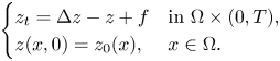
In this paper, we consider the following chemotaxis system with anisotropic porous medium-type diffusion:
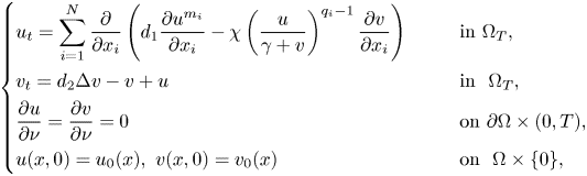
where $\Omega _{T}=\Omega \times (0,T)$ , $T>0$
 is a fixed time, $\Omega$
 is a bounded domain in $\mathbb {R}^{N}$
 , $N\geq 3$
 with smooth boundary $\partial \Omega$
 , $q_{i}\geq 2$
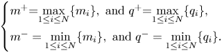
 and $m^{-}>q_{i}-\frac {2}{N}$
 for all $i=1,..,N$
 , such that
The positive constant $\chi$ is called the chemotaxis coefficient, $d_{1},d_{2}>0$
 are the diffusion coefficients and $\gamma \geq 1$
 .
.
In general, organism or cell moves from a lower concentration towards a higher concentration of the chemo attractant, which is known as positive chemotaxis. In the same way, the opposite movement of the organisms is known as negative chemotaxis. In particular, microorganisms use chemotaxis to position themselves within the optimal portion of their habitats by monitoring the environmental concentration gradients of specific chemical attractant (positive chemotaxis) and repellent ligands (negative chemotaxis). Famous examples of biological species experiencing chemotaxis are the flagellated bacteria Salmonella typhimurium and Escherichia coli, the slime mould amoebae Dictyostelium discoideum and the human endothelial cells (see [Reference Adler1, Reference Bonner4, Reference Eisenbach6]). Theoretical and mathematical modelling of chemotaxis phenomena dates back to the pioneering works of Patlak in 1950s [Reference Patlak20] and Keller–Segel in 1970s [Reference Keller and Segel18]. A general form of Patlak–Keller–Segel model for chemotaxis is given by
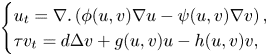
where $u$ denotes the density of cell population and $v$
 is the chemical attractant concentration. The mobility function $\phi (u,v)$
 describes the diffusivity of the cells and $\psi (u,v)$
 represents the chemotaxis sensibility, while the functions $g(u,v)$
 and $h(u,v)$
 are kinetic functions that describe production and degradation of the chemical signal, respectively. When $\phi (u,v)=1$
 and $\tau >0$
 , system (1.2) becomes the classical parabolic–parabolic Keller–Segel system, such system has been extensively studied, see for example [Reference Tao27, Reference Tao and Winkler28, Reference Yan and Li32] and references therein. For the study of the parabolic-elliptic Keller–Segel system of quasilinear type, namely $\tau =0$
 , with general $\phi (u,v)$
 in (1.2), we refer to [Reference Sugiyama23–Reference Sugiyama and Kunii25] and references therein.
Equation (1.1) with $m_i=m$ and $q_i=q$
 is sometimes called the equation of isotropic diffusion. In the case of degenerate diffusion, the model $\phi (u,v)=mu^{m-1}$
 and $\psi (u,v)=u^{q-1}$
 in $\mathbb {R}^{N}$
 was studied by several authors. The existence of the weak solutions was shown when $q-m<0$
 in [Reference Sugiyama and Kunii25] and when $q-m<\frac {2}{N}$
 in [Reference Ishida and Yokota13]. When $q-m\geq \frac {2}{N}$
 and the initial data $(u_{0},v_{0})$
 is small in some sense, the existence of the weak solutions was proved in [14], whereas, if $q-m>\frac {2}{N}$
 then blow-up of solutions as in [Reference Winkler30] was studied in [Reference Ishida, Ono and Yokota15, Reference Ishida and Yokota16].
In the present work, we are interested in the anisotropic case where the diffusion rates differ according to the direction $x_i$ . Despite the resemblance with the isotropic cases presented in the previous mentioned works, the properties of the solutions to anisotropic equations are in striking contrast with the properties of the classical isotropic equations. The difficulties brought in by the anisotropy and the inhomogeneity of the diffusion operator are illustrated by the analysis of the self-similar solutions of anisotropic porous medium and $\vec {p}$
 -Laplacian types [Reference Antontsev and Shmarev2, Reference Antontsev and Shmarev3, Reference Düzgün, Mosconi and Vespri5]. Unlike the isotropic case where the typical geometry is defined in terms of balls in $\mathbb {R}^{N}$
 , in the anisotropic case it is defined by parallelepipeds with the edge lengths related to the exponents $m_i$
 and $q_i$
 .
.
The chemotaxis model with anisotropic porous medium diffusion type is motivated from a biological point of view [Reference Szymanska, Morales-Rodrigo, Lachowicz and Chaplain26]. It is worthy of mentioning that the porous medium type diffusion can represent population pressure in cell invasion models [Reference Rosen21], which initially arises from the ecology literature [Reference Gurney and Nisbet12, Reference Xu, Ji, Jin, Mei and Yin31]. In fact, experimental investigation has shown that the diffusion coefficient depends on the bacterial density [Reference Wakita, Komatsu, Nakahara, Matsuyama and Matsushita29]. In the bacterial experiments done by Ohgiwari, Matsushita and Matsuyama [Reference Ohgiwari, Matsushita and Matsuyama19], they recognized that cells located inside the bacterial colonies move actively, but cells became sluggish at the outermost front with apparently low cell density. This phenomenon indicates that bacteria become active as the cell density $u$ increases. Thus, a natural choice of the bacterial diffusion coefficient is $\phi (u,v)=m_{i}u^{m_{i}-1}$
 with $m_{i}>1$
 for all $i=1,..,N$
 , and this porous medium type bacterial diffusivity is based on the degenerate diffusion model proposed by Kawasaki et al. [Reference Kawasaki, Mochizuki, Matsushita, Umeda and Shigesada17]. To our knowledge, Keller–Segel system with anisotropic porous medium diffusion models has not been studied specially and systematically.
2. Preliminary and main result
2.1 Imbedding and technical lemmas
To derive our existence and regularity results, we will need the following
Theorem 2.1 [Reference Esfahani9], Theorem 1.1. Let $N\geq 2$ , $\alpha _{j}\in (0,1)$
 , $1\leq p< q$
 and $p_{j}\geq 1$
 , $j=1,..,N$
 , be such that $\displaystyle \sum _{j=1}^{N}\frac {1}{\alpha _{j}p_{j}}>1$
 . Then, for $u\in W^{(\alpha ),(p,\vec {p})}(\mathbb {R}^{N})$
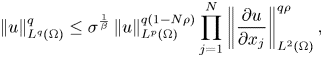
 (The fractional Sobolev–Liouville space) the inequality
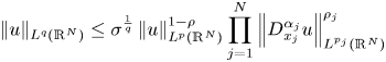
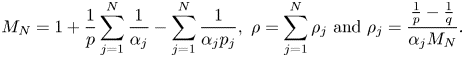
hold provided $M_{N}>0$ and
and
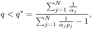
where
The following lemma will show that theorem 2.1 holds true even for the case where $0< p<1$ and $p_{j}=2,~\forall j=1,..,N$
 .
.
Lemma 2.2 Let $\Omega \subset \mathbb {R}^{N}$ with $N\geq 3$
 be a bounded domain with smooth boundary, and $0< p<1\leq q<\frac {2N}{N-2}$
 . Then, for all $u\in H^{1}(\Omega )$
 we have
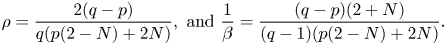
where $\rho =\frac {2(q-p)}{q(p(2-N)+2N)}$ , and $\frac {1}{\beta }=\frac {(q-p)(2+N)}{(q-1)(p(2-N)+2N)}$
 .
.
Proof. By Hölder's inequality , we get that

Then, by using theorem 1 of section 5.4 in [Reference Evans10] and applying theorem 2.1 for $p=1$ and $p_{j}=2,~\forall j=1,..,N$
 , we obtain
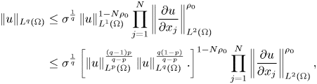
where $\rho _{0}=\frac {1-\frac {1}{q}}{N(\frac {1}{N}+\frac {1}{2})}$ . Then from (2.3) we get (2.2) with
□
Possible references on the theory of anisotropic Sobolev spaces are in [Reference El Bahja7, Reference El Bahja8] and references therein. Next, we give some fundamental estimates of solutions to the following Cauchy problem for inhomogeneous linear heat equations:
The following lemma can be found in [14].
Lemma 2.3 Let $\Omega \subset \mathbb {R}^{N}$ with $N\in \mathbb {N}$
 be a bounded domain with smooth boundary, $T>0$
 , $1\leq p\leq \infty$
 and $z_{0}\in L^{p}(\Omega )$
 . If $f\in L^{1}(0,T; L^{p}(\Omega ))$
 , then (2.4) has a unique mild solution $z\in C([0,T]; L^{p}(\Omega ))$
 given by
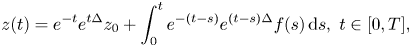
where $(e^{t\Delta }f)(x,t)=(4\pi t)^{-\frac {N}{2}}\int _{\Omega }e^{-\frac {|x-y|^{2}}{4t}}f(y,t)~dy$ . Moreover, the following estimates hold.
• Let $1\leq q\leq p\leq \infty$
 and $\frac {1}{q}-\frac {1}{p}<\frac {1}{N}$. Assume further that $z_{0}\in W^{2,p}(\Omega )$ and $f\in L^{\infty }(0,T; W^{1,q}(\Omega ))$. Then for every $t\in [0,T]$,
(2.6)\begin{align} & \|z(t)\|_{L^{p}(\Omega)}\leq\|z_{0}\|_{L^{p}(\Omega)}+C_{0}\|f\|_{L^{\infty}(0,T;L^{q}(\Omega))}, \end{align}
(2.7)\begin{align} & \|\nabla z(t)\|_{L^{p}(\Omega)}\leq\|\nabla z_{0}\|_{L^{p}(\Omega)}+C_{0}\|f\|_{L^{\infty}(0,T;L^{q}(\Omega))}, \end{align}
(2.8)\begin{align} & \|\Delta z(t)\|_{L^{p}(\Omega)}\leq\|\Delta z_{0}\|_{L^{p}(\Omega)}+C_{0}\|\nabla f\|_{L^{\infty}(0,T;L^{q}(\Omega))}, \end{align}where $C_{0}$
is a positive constant depending on $p,q$ and $N$.
and $\frac {1}{q}-\frac {1}{p}<\frac {1}{N}$. Assume further that $z_{0}\in W^{2,p}(\Omega )$ and $f\in L^{\infty }(0,T; W^{1,q}(\Omega ))$. Then for every $t\in [0,T]$,
(2.6)\begin{align} & \|z(t)\|_{L^{p}(\Omega)}\leq\|z_{0}\|_{L^{p}(\Omega)}+C_{0}\|f\|_{L^{\infty}(0,T;L^{q}(\Omega))}, \end{align}
(2.7)\begin{align} & \|\nabla z(t)\|_{L^{p}(\Omega)}\leq\|\nabla z_{0}\|_{L^{p}(\Omega)}+C_{0}\|f\|_{L^{\infty}(0,T;L^{q}(\Omega))}, \end{align}
(2.8)\begin{align} & \|\Delta z(t)\|_{L^{p}(\Omega)}\leq\|\Delta z_{0}\|_{L^{p}(\Omega)}+C_{0}\|\nabla f\|_{L^{\infty}(0,T;L^{q}(\Omega))}, \end{align}where $C_{0}$
is a positive constant depending on $p,q$ and $N$.• Let $1< p<\infty$
and $f\in L^{p}(0,T;L^{p}(\Omega ))$. Then for every $t\in [0,T]$,
(2.9)\begin{equation} \|\Delta z(t)\|_{L^{p}(0,t;L^{p}(\Omega))}\leq\|\Delta z_{0}\|_{L^{p}(\Omega)}\left(1-e^{{-}pt}\right)^{\frac{1}{p}}+C_{ }\|f\|_{L^{p}(0,T;L^{p}(\Omega))}, \end{equation}where $C_{0}$
is a positive constant depending on $N$ and $p$.


2.2 Formulation of the problem and main result
Throughout this paper, we deal with weak solutions of (1.1). Our definition of the weak solutions now reads
Definition 2.4 A pair of nonnegative functions $(u,v)$ is said to be a weak solution of (1.1) if and only if for all $i=1,..,N$
 we have

such that $(u,v)$ satisfies the equations in the sense of distribution, i.e., that
for any continuously differentiable function $\varphi$ with compact support in $\Omega \times [0,T)$
 .
.
Motivated by the works mentioned in the previous section, our paper extends the results in [14, Reference Sugiyama and Kunii25] to the system (1.1) with anisotropic nonlinear diffusion. Now we state the main result of this paper. To be precise, we will assume the initial data $(u_{0},v_{0})$ to satisfy

Theorem 2.5 Let $q_{i}\geq 2$ and $m^{-}>q_{i}-\frac {2}{N}$
 for every $i=1,..N$
 , $\Omega \subset \mathbb {R}^{N}$
 for $N\geq 3$
 be a bounded domain with smooth boundary. Then for all $(u_{0},v_{0})$
 satisfying (2.10), the system (1.1) possesses at last one weak solution in the sense of definition 2.4.
3. Approximated equations
The first equation of (1.1) is a quasilinear parabolic equation of degenerate type. Therefore, we cannot expect the system (1.1) to have a classical solution at the point where $u$ vanishes. In order to prove theorem 2.5, we use a compactness method and introduce the following approximated equation of (1.1):

where $\varepsilon \in (0,1)$ .
.
3.1 Existence of weak solutions of (3.1)
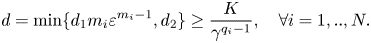
We are going to give an existence result of (3.1) under the condition that there exists a positive constant $k$ such that
Theorem 3.1 Assume that (3.2) holds. If $u_{0},v_{0}\in L^{2}(\Omega )$ , then (3.1) possesses a nonnegative weak solution $(u_{\varepsilon },v_{\varepsilon })$
 such that

such that $u_{\varepsilon }$ has the conservation law

Proof. The existence of the weak solution to (3.1) can be obtained by using Schauder's fixed point theorem, a priori estimates and using the compactness results. We start by introducing for a small number $\delta >0$ the following

such that we have $0\leq f_{\delta }(s)\leq \min \{s^+,\frac {1}{\delta }\}$ for any $s\in \mathbb {R}$
 and $f_{\delta }(s)\longrightarrow s$
 pointwise in $\mathbb {R}$
 as $\delta \longrightarrow 0$
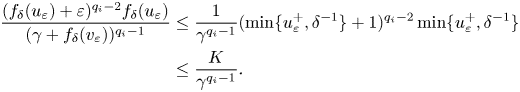
 . Therefore, we can conclude that there exists a positive constant $K$
 such that
Let $\overline {u}_{\varepsilon },\overline {v}_{\varepsilon }\in L^{2}(\Omega _{T})$ be given and consider the linear problem
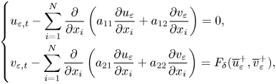
where the diffusion matrix $A _{i}=(a_{jk})_{i}$ is given by

Moreover, the matrix $A _{i}$ is uniformly positive definite, since for any $X=(x,y)\in \mathbb {R}^{2}$
 we have
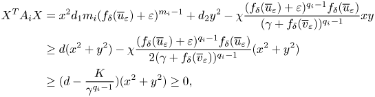
where we used (3.2) and the fact that $xy=\frac {1}{2}(x+y)^{2}-\frac {1}{2}(x^{2}+y^{2})\geq -\frac {1}{2}(x^{2}+y^{2})$ and $-xy=\frac {1}{2}(x-y)^{2}-\frac {1}{2}(x^{2}+y^{2})\geq -\frac {1}{2}(x^{2}+y^{2})$
 . Hence, the desired existence result is guaranteed by theorem 1 in [Reference Galiano, Garzón and Jüngel11].
3.2 A priori estimates
In order to prove theorem 2.5, we state and prove two key propositions which control $L^{r}-$ and $L^{\infty }-$
 estimates of the solution $(u_{\varepsilon },v_{\varepsilon })$
 of (3.1).
Proposition 3.2 Assume that (2.10), and (3.2) hold. Let $N\geq 3$ , $q_{i}\geq 2$
 and $m^{-}>q_{i}-\frac {2}{3}$
 for all $i=1,..,N$
 . Then $(u_{\varepsilon },v_{\varepsilon })$
 satisfies the following estimates


where $C$ is a positive constant independent of $\varepsilon$
 .
.
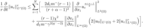
Proof. By taking $r\in (1,\infty )$ , multiplying the first equation in (3.1) by $u_{\varepsilon }^{r-1}$
 and integrating by parts, we get
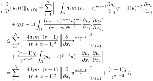
where
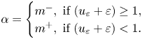
Next, we set
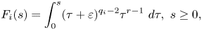
such that

Therefore, $I_{i}$ becomes
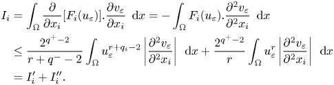
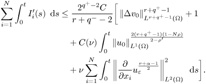
Next, we are going to integrate $I_{i}'$ over $(0,t)$
 for $t\in (0,T)$
 such that
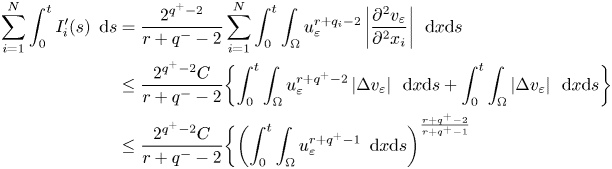
where we used Hölder's inequality, (2.9) and Young's inequality.
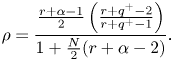
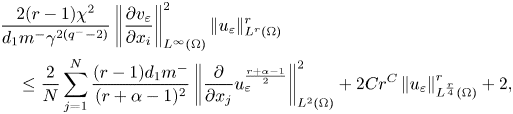
Next, we are going to simplify the last integral in the right-hand side of (3.9) by using lemma 2.2. As a consequence, by letting $r>r_{0}\!=\!\max \{\alpha -2q^+\!+\!1,\frac {N}{2}(q^+-\alpha ) -q^++1,\frac {2(N-1)}{N}-\alpha \}$ , we have the following
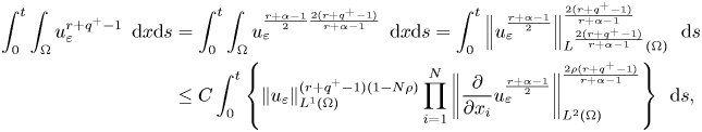
where
We can replace the geometric mean on the right-hand side of (3.10) by an arithmetic mean. Indeed, by the inequality between geometric and arithmetic means we get
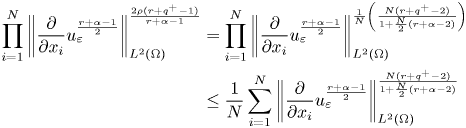
Since, we took $q_{i}<\frac {2}{N}+m^{-}\leq \frac {2}{N}+\alpha$ for all $i=1,..,N$
 . Then we get
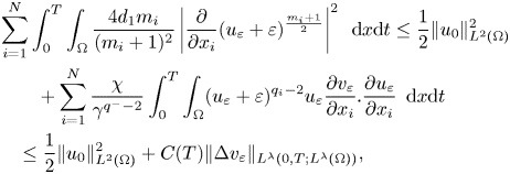
Therefore, by using (3.11), (3.12), Young's inequality and the mass conservation law (3.3), we obtain
The integral $I''_{i}$ can be controlled by the same way as $I'_{i}$
 for all $i=1,..,N$
 . Consequently, we omit that $\sum _{i}^{N}\int _{0}^{t}I''_{i}~\,{\rm d}s$
 satisfy the same estimation as in (3.13). Therefore, by integrating (3.6) over $(0,t)$
 and using the previous estimates, we arrive at
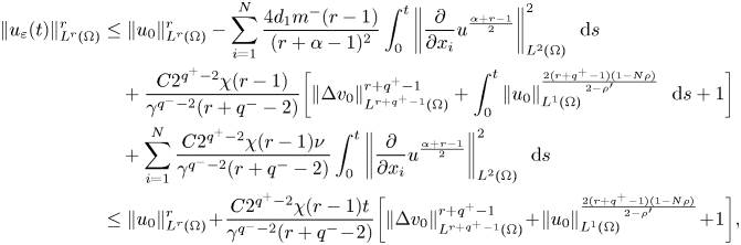
where we took $\nu =\frac {4d_{1}m^{-}\gamma ^{q^{-}-2}(r+q^{-}-2)}{2^{q^+-2}C\chi (r+\alpha -1)^{2}}$ . Moreover, by letting $r>r_{1}=\{r_{0},\beta -q^++1\}$
 for $\beta > > 1$
 , we obtain that
where $C$ is a positive constant independent of $\varepsilon$
 .
.
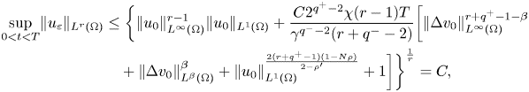
Now, for the case $1\leq r\leq r_{1}$ we have the following

where we used Hölder's inequality, the mass conservation law (3.3) and Young's inequality. Hence, (3.15) and (3.16) give us the desired estimation for every $r\in [1,\infty )$ .
.
Finally estimation (3.5) is a direct consequence of (2.6), (2.7) and (3.4) with $r=N+1$ .
.
We conclude this section with the proof of $L^{\infty }$ -estimates of the approximated solutions.
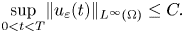
Proposition 3.3 Let the same assumptions as those in proposition 3.2 hold. Then, there exists a positive constant $C$ independent of $\varepsilon$
 such that
Proof. We begin by multiplying the first equation in (3.1) by $u_{\varepsilon }^{r-1}$ such that
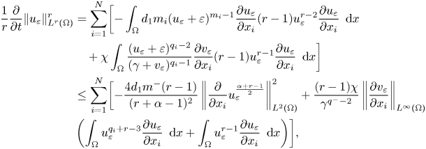
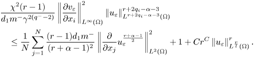
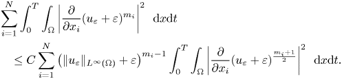
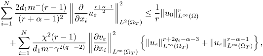
where $\alpha$ is defined in (3.7). Next, we are going to simplify the last two integrals in the right-hand side of (3.18). Then, for all $i=1,..,N$
 we have

where we used Young's inequality and choose $\nu$ accordingly.
We will deal only with the norm $\left \| u_{\varepsilon } \right \|_{L^{r+2q_{i}-\alpha -3}(\Omega )}^{r+2q_{i}-\alpha -3}$ in the right-hand side of (3.19), because the last norm can be controlled by the same way. Furthermore, we are going to study the following two possible cases.
Case 1: $q_{i}>3-\frac {2}{N},~\forall i=1,..,N.$
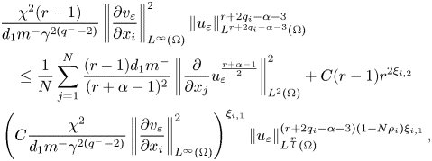
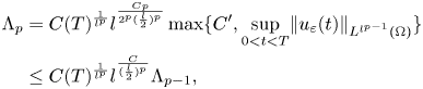
Let $l$ be a natural number which is chosen later. Therefore, by applying lemma 2.2, we obtain
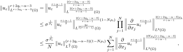
for $r\!>\!r_{0}=\max \{3\alpha -4q_{i}+5, -\frac {N}{2}(\alpha -1)+\frac {(N-2)}{2}(2q_{i}-\alpha -3),\alpha -2q_{i}+3\}, l\!>\!1$ ,
,
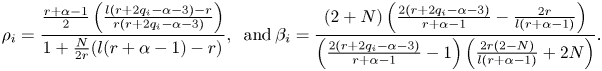
By simple computation, we find that $\frac {2N\rho _{i}(r+2q_{i}-\alpha -3)}{r+\alpha -1}<2$ and $\frac {1}{\beta _{i}}\leq 6$
 for every $r>r_{0}$
 and $i=1,..,N$
 . Therefore, by Young's inequality we get

where

Next, by taking $\nu =\frac {d_{1}m^{-}}{(r+\alpha -1)^{2}}$ , then $\displaystyle C(\nu )=\frac {1}{q_{i}(\nu p_{i})^{\frac {q_{i}}{p_{i}}}}$
 , where

Then, (3.21) becomes
where

Next, for $l>1$ , $r>r_{0}$
 and for every $i=1,..N$
 , we have
Consequently, we obtain that

Then, by (3.24) we get the following estimations

Therefore, (3.22) becomes
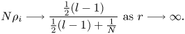
Next, we are going to simplify the last term in the right-hand side of (3.25). For this reason, we choose $l$ to verify

such that
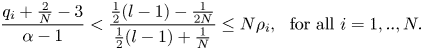
Therefore, by taking

we get that

By simple computation, we get also $\xi _{i,3}\leq Nl+2$ for all $i=1,..,N$
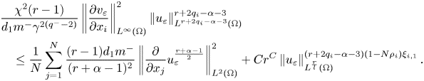
 . To this end, we apply Young's inequality on the last term in the right-hand side of (3.25) such that
By the same method, we get also that
for every $r>r_{1}$ . Then, by putting (3.26) and (3.27) into (3.18) we obtain
Integrating (3.28) from 0 to $t$ , we obtain

Since
Then,

We are now in a position to derive the claimed $L^{\infty }-$ estimate. Therefore, we set

Thereafter, we take $r=l^{p}$ in (3.31) which leads to
since $p\leq 2^{p}$ for $p\geq 1$
 . By induction, we get
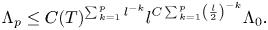
Then, by using the mass conservation law (3.3), taking $l>2$ and letting $p\longrightarrow \infty$
 , we arrive at

where $C''$ is a positive constant independent of $\varepsilon$
 .
.
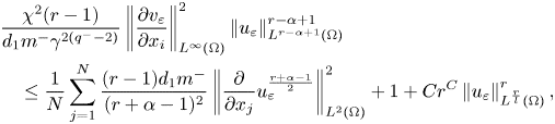
Case 2: $2\leq q_{i}\leq 3-\frac {2}{N},~\forall i=1,..,N.$
Knowing that $q_{i}<\alpha +\frac {2}{N}$ , then $2q_{i}<\alpha +3$
 for every $i=1,..,N$
 . Therefore,

Then, (3.18) becomes
Thereafter, by applying lemma 2.2 once again we obtain
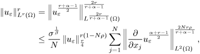
where

It is easy to verify that $\frac {2Nr\rho }{r+\alpha -1}<2$ and $\frac {1}{\beta }\leq 6$
 for suitable $r>0$
 . Then, by using the same method we used to get (3.27), we obtain
for suitable $r>0$ . Hence, by putting (3.37) into (3.35) and applying similar arguments of the case $q>3-\frac {2}{N}$
 we get the desired $L^{\infty }-$
 estimate.
We complete this section by discussing some uniform estimates (with respect to $\varepsilon$ ) of $u_{\varepsilon }$
 and $v_{\varepsilon }$
 .
.
Lemma 3.4 For $q_{i}\geq 2$ and $m^{-}>q_{i}-\frac {2}{N}$
 for all $i\!=\!1,..N$
 , there exists a constant $C$
 such that
and,
for each $\varepsilon \in (0,1)$ and $\beta$
 a big enough positive constant.
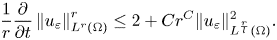
Proof. We multiply the first equation of (3.1) by $u_{\varepsilon }$ and integrate over $\Omega \times (0,T)$
 such that
where we used the same method we introduced to get (3.8), applying proposition 3.17 and for $\lambda > > 1$ . Therefore, by (2.9) we get (3.8). Moreover, we note that
Then, (3.39) follows from (3.38).
Next, taking $\varphi \in C^{\infty }(\Omega _{T})$ , multiplying the first equation of (3.1) by $\beta u_{\varepsilon }^{\beta -1}\varphi$
 , and integrating by parts, we obtain

where we used proposition 3.3, the embedding of $W^{1,N+1}(\Omega )$ into $L^{\infty }(\Omega )$
 , and (3.38). Thus, we get (3.40). Also, by the same method and using (3.5) and (3.17) we get (3.41).
4. Proof of theorem 2.5
The goal of this section is to prove theorem 2.5. In the proof, we need the strong convergence of $u_{\varepsilon }$ and $v_{\varepsilon }$
 . Then, from (3.18), (3.19), proposition 3.3 and integrating over $(0,T)$
 , we get
for suitable $r$ . Therefore, by taking $r=2\beta -\alpha +1$
 in (4.1) and using (3.5) and proposition 3.3 we get that $u_{\varepsilon }^{\beta }\in L^{2}(0,T;H^{1}(\Omega ))$
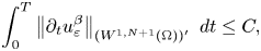
 while $\partial _{t}u_{\varepsilon }^{\beta }$
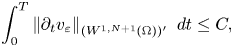
 is bounded in $L^{1}(0,T;(W^{1,N+1}(\Omega ))')$
 by lemma 3.4. Since $H^{1}(\Omega )$
 is compactly embedded in $L^{2}(\Omega )$
 and $L^{2}(\Omega )$
 is continuously embedded in $(W^{1,N+1}(\Omega ))'$
 , it follows from corollary 4 in [Reference Simon22] that $u_{\varepsilon }^{\beta }$
 is compact in $L^{2}(0,T;L^{2}(\Omega ))$
 . Since $u_{\varepsilon }\longmapsto u_{\varepsilon }^{\frac {1}{\beta }}$
 is Hölder continuous with exponent $\frac {1}{\beta }$
 , we get that $u_{\varepsilon }$
 is compact in $L^{2\beta }(0,T;L^{2\beta }(\Omega ))$
 . Thus, there exist a function $u\in L^{2\beta }(0,T;L^{2\beta }(\Omega ))$
 and a subsequence $(\varepsilon _{n})_{n\geq 1}$
 such that

This gives
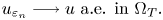
On the other hand, by proposition 3.3 we get that
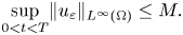
As a consequence, we get that
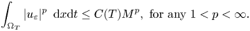
Therefore, by using Lebesgue dominated convergence theorem, (4.3) and (4.5), we obtain

By using the following inequality

we get
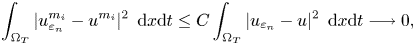
where we used (4.6) for $p=2$ . Then, we get that

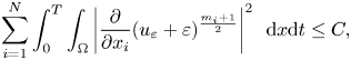
Since $\frac {\partial u^{m_{i}}}{\partial x_{i}}$ is bounded in $L^{2}(0,T;L^{2}(\Omega ))$
 by (3.39), and using (4.9) we arrive at
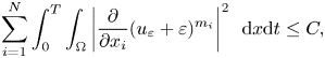
for any $i=1,..,N$ . Thereafter, by using (3.5), (3.41) and the same method we used to get (4.6), we obtain

and
Using (4.6), (4.11), (4.7) for $q_{i}-1$ instead of $m_{i}$
 , and since $q_i\geq 2$
 and $\gamma \geq 1$
 we get that

Integrating (3.1) with respect to $x$ and $t$
 , we see that $(u_{\varepsilon _{n}},v_{\varepsilon _{n}})$
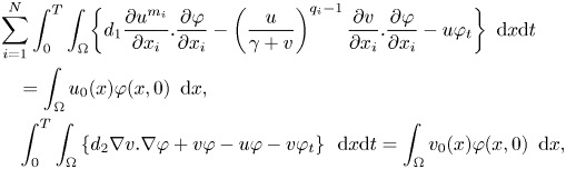
 satisfies

for any continuously differentiable function $\varphi$ with compact support in $\Omega \times [0,T)$
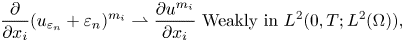
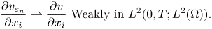
 . Wherefore, by using (4.6), (4.9), (4.10), (4.11), (4.12), (4.13) and by the standard convergence argument we obtain
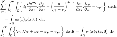
where $q_{i}\geq 2$ and $m^{-}>q_{i}-\frac {2}{N}$
 for any $i=1,..,N$
 . Hence, we conclude the proof of theorem 2.5.

