


1 Introduction
The multicut problem (Hu Reference Hu1963) involves finding a set of edges from an undirected graph G such that each given source–sink pair in
 $\mathcal{P}$
is disconnected in the graph after removing these edges; this approach has a variety of applications in VLSI design (Costa et al. Reference Costa, Létocart and Roupin2005; Zhang et al. Reference Zhang, Zhu and Luan2012) and computer vision (Keuper et al. Reference Keuper, Andres and Brox2015; Tang et al. Reference Tang, Andriluka, Andres and Schiele2017). When
$\mathcal{P}$
is disconnected in the graph after removing these edges; this approach has a variety of applications in VLSI design (Costa et al. Reference Costa, Létocart and Roupin2005; Zhang et al. Reference Zhang, Zhu and Luan2012) and computer vision (Keuper et al. Reference Keuper, Andres and Brox2015; Tang et al. Reference Tang, Andriluka, Andres and Schiele2017). When
 $|\mathcal{P}|=1$
, this problem is referred to as the famous minimum cut problem and admits a polynomial-time algorithm; when
$|\mathcal{P}|=1$
, this problem is referred to as the famous minimum cut problem and admits a polynomial-time algorithm; when
 $|\mathcal{P}|=2$
, this problem can also be solved in polynomial time (Hu Reference Hu1963). When
$|\mathcal{P}|=2$
, this problem can also be solved in polynomial time (Hu Reference Hu1963). When
 $|\mathcal{P}|=3$
, this problem is NP-hard (Dahlhaus et al. Reference Dahlhaus, Johnson, Papadimitriou, Seymour and Yannakakis1994), and when
$|\mathcal{P}|=3$
, this problem is NP-hard (Dahlhaus et al. Reference Dahlhaus, Johnson, Papadimitriou, Seymour and Yannakakis1994), and when
 $|\mathcal{P}|$
is arbitrary, this problem is NP-hard to approximate within any constant factor assuming the unique games conjecture (Chawla et al. Reference Chawla, Krauthgamer, Kumar, Rabani and Sivakumar2006). Garg et al. (Reference Garg, Vazirani and Yannakakis1996) constructed an
$|\mathcal{P}|$
is arbitrary, this problem is NP-hard to approximate within any constant factor assuming the unique games conjecture (Chawla et al. Reference Chawla, Krauthgamer, Kumar, Rabani and Sivakumar2006). Garg et al. (Reference Garg, Vazirani and Yannakakis1996) constructed an
 $O(\log |\mathcal{P}|)$
-approximation algorithm by using the LP rounding technique, while Zhang (Reference Zhang2022) constructed a
$O(\log |\mathcal{P}|)$
-approximation algorithm by using the LP rounding technique, while Zhang (Reference Zhang2022) constructed a
 $\sqrt{|\mathcal{P}|}$
-approximation algorithm by using the LP rounding-plus-greedy method.
$\sqrt{|\mathcal{P}|}$
-approximation algorithm by using the LP rounding-plus-greedy method.
The multicut problem in general graphs is complex. To address this problem more effectively, researchers have shifted their focus to trees, which are special graphs. The multicut problem in trees (Garg et al. Reference Garg, Vazirani and Yannakakis1997) and its generalizations have been widely studied, such as the partial multicut problem in trees (Golovin et al. Reference Golovin, Nagarajan and Singh2006; Levin and Segev Reference Levin and Segev2006), the generalized partial multicut problem in trees (Könemann et al. Reference Könemann, Parekh and Segev2011), the prized-collection multicut problem in trees (Levin and Segev Reference Levin and Segev2006), the multicut problem in trees with submodular penalties (Liu and Li Reference Liu and Li2022), and the k-prize-collecting multicut problem in trees (Hou et al. Reference Hou, Liu and Hou2020).
Inspired by Könemann et al. (Reference Könemann, Parekh and Segev2011) and Xu et al. (Reference Xu, Wang, Du and Wu2016), in this paper, we study the K-prize-collecting multicut problem in trees with submodular penalties (K-PCMTS), which is a generalization of all the problems in trees mentioned above. In the K-PCMTS, we are given a tree
 $T=(V,E)$
, a set
$T=(V,E)$
, a set
 $\mathcal{P}=\{(s_1,t_1),(s_2,t_2),\ldots, (s_m,t_m)\}$
of m source–sink pairs of vertices in V, and a profit lower bound K. Each edge
$\mathcal{P}=\{(s_1,t_1),(s_2,t_2),\ldots, (s_m,t_m)\}$
of m source–sink pairs of vertices in V, and a profit lower bound K. Each edge
 $e\in E$
is associated with a cost
$e\in E$
is associated with a cost
 $c_e$
, and each pair
$c_e$
, and each pair
 $(s_j,t_j)\in \mathcal{P}$
is associated with a profit
$(s_j,t_j)\in \mathcal{P}$
is associated with a profit
 $p_j$
. For any
$p_j$
. For any
 $M\subseteq E$
, let c(M) be the total cost of the edges in M and
$M\subseteq E$
, let c(M) be the total cost of the edges in M and
 $R_M$
be the set of pairs still connected after removing M. The problem is to find a partial multicut
$R_M$
be the set of pairs still connected after removing M. The problem is to find a partial multicut
 $M\subseteq E$
such that the total profit of the disconnected pairs after removing M is at least K, and the objective value, i.e.,
$M\subseteq E$
such that the total profit of the disconnected pairs after removing M is at least K, and the objective value, i.e.,
 $c(M)+\pi(R_M)$
, is minimized, where the penalty is determined by a given nondecreasing submodular function
$c(M)+\pi(R_M)$
, is minimized, where the penalty is determined by a given nondecreasing submodular function
 $\pi:2^{\mathcal{P}}\rightarrow \mathbf{R}_{\geq 0}$
, which has the property of decreasing marginal returns (Fujishige Reference Fujishige2005; Li et al. Reference Li, Du, Xiu and Xu2015).
$\pi:2^{\mathcal{P}}\rightarrow \mathbf{R}_{\geq 0}$
, which has the property of decreasing marginal returns (Fujishige Reference Fujishige2005; Li et al. Reference Li, Du, Xiu and Xu2015).
1.1 Related works
When
 $K=\sum_{j:(s_j,t_j)\in \mathcal{P}}p_j$
, which implies that all pairs must be disconnected, the K-PCMTS is exactly the multicut problem in trees. Garg et al. (Reference Garg, Vazirani and Yannakakis1997) proved that this problem is NP-hard, and they presented a 2-approximation algorithm based on a primal-dual technique. In the same paper, they also proved that the multicut problem in trees is at least as hard to approximate as the vertex cover problem, which cannot be approximated within
$K=\sum_{j:(s_j,t_j)\in \mathcal{P}}p_j$
, which implies that all pairs must be disconnected, the K-PCMTS is exactly the multicut problem in trees. Garg et al. (Reference Garg, Vazirani and Yannakakis1997) proved that this problem is NP-hard, and they presented a 2-approximation algorithm based on a primal-dual technique. In the same paper, they also proved that the multicut problem in trees is at least as hard to approximate as the vertex cover problem, which cannot be approximated within
 $2-\varepsilon$
for any
$2-\varepsilon$
for any
 $\varepsilon> 0$
under the unique games conjecture (Khot and Regev Reference Khot and Regev2008). Thus, the approximation factor of the algorithm in Garg et al. (Reference Garg, Vazirani and Yannakakis1997) is the best.
$\varepsilon> 0$
under the unique games conjecture (Khot and Regev Reference Khot and Regev2008). Thus, the approximation factor of the algorithm in Garg et al. (Reference Garg, Vazirani and Yannakakis1997) is the best.
When
 $\pi(R)=0$
for any
$\pi(R)=0$
for any
 $R\subseteq \mathcal{P}$
, i.e., the objective value of a partial multicut M is c(M), and the K-PCMTS is equivalent to the generalized partial multicut problem for trees (Könemann et al. Reference Könemann, Parekh and Segev2011), in which the problem is to find a minimum cost edge set
$R\subseteq \mathcal{P}$
, i.e., the objective value of a partial multicut M is c(M), and the K-PCMTS is equivalent to the generalized partial multicut problem for trees (Könemann et al. Reference Könemann, Parekh and Segev2011), in which the problem is to find a minimum cost edge set
 $M\subseteq E$
such that the total profit of the disconnected pairs is at least K. Könemann et al. (Reference Könemann, Parekh and Segev2011) presented an
$M\subseteq E$
such that the total profit of the disconnected pairs is at least K. Könemann et al. (Reference Könemann, Parekh and Segev2011) presented an
 $(\frac{8}{3}+\varepsilon)$
-approximation algorithm for this problem, where
$(\frac{8}{3}+\varepsilon)$
-approximation algorithm for this problem, where
 $\varepsilon>0$
is any small constant. When
$\varepsilon>0$
is any small constant. When
 $\pi(R)=0$
for any
$\pi(R)=0$
for any
 $R\subseteq \mathcal{P}$
and
$R\subseteq \mathcal{P}$
and
 $p_j=1$
for any
$p_j=1$
for any
 $(s_j,t_j)\in \mathcal{P}$
, the K-PCMTS is equivalent to the partial multicut problem in trees. Given any small constant
$(s_j,t_j)\in \mathcal{P}$
, the K-PCMTS is equivalent to the partial multicut problem in trees. Given any small constant
 $\varepsilon>0$
, Levin and Segev (Reference Levin and Segev2006) and Golovin et al. (Reference Golovin, Nagarajan and Singh2006) independently presented a polynomial-time
$\varepsilon>0$
, Levin and Segev (Reference Levin and Segev2006) and Golovin et al. (Reference Golovin, Nagarajan and Singh2006) independently presented a polynomial-time
 $(\frac{8}{3}+\varepsilon)$
-approximation algorithm for the partial multicut in trees based on the Lagrangian relaxation technique. By more carefully analyzing the relaxation technique, Mestre (Reference Mestre2008) was able to provide an improved polynomial-time
$(\frac{8}{3}+\varepsilon)$
-approximation algorithm for the partial multicut in trees based on the Lagrangian relaxation technique. By more carefully analyzing the relaxation technique, Mestre (Reference Mestre2008) was able to provide an improved polynomial-time
 $(2+\varepsilon)$
-approximation algorithm.
$(2+\varepsilon)$
-approximation algorithm.
When
 $K=0$
, the K-PCMTS reduces the multicut problem in trees with submodular penalties (Liu and Li Reference Liu and Li2022), in which the problem is to find a partial multicut M such that
$K=0$
, the K-PCMTS reduces the multicut problem in trees with submodular penalties (Liu and Li Reference Liu and Li2022), in which the problem is to find a partial multicut M such that
 $c(M)+\pi(R_M)$
is minimized. Liu and Li (Reference Liu and Li2022) presented a combinatorial polynomial-time 3-approximation algorithm based on a primal-dual scheme for this problem. When
$c(M)+\pi(R_M)$
is minimized. Liu and Li (Reference Liu and Li2022) presented a combinatorial polynomial-time 3-approximation algorithm based on a primal-dual scheme for this problem. When
 $K=0$
and the penalty function is linear, i.e.,
$K=0$
and the penalty function is linear, i.e.,
 $\pi(R)=\sum_{j:(s_j,t_j)\in R}\pi(\{(s_j,t_j)\})$
for any
$\pi(R)=\sum_{j:(s_j,t_j)\in R}\pi(\{(s_j,t_j)\})$
for any
 $R\subseteq \mathcal{P}$
, the K-PCMTS is equivalent to the prized-collecting multicut problem in trees (Levin and Segev Reference Levin and Segev2006); there is a polynomial-time 2-approximation algorithm for that scenario.
$R\subseteq \mathcal{P}$
, the K-PCMTS is equivalent to the prized-collecting multicut problem in trees (Levin and Segev Reference Levin and Segev2006); there is a polynomial-time 2-approximation algorithm for that scenario.
When the penalty function is linear, the K-PCMTS is exactly the K-prize-collecting multicut problem in trees. Based on the method in Guo et al. (Reference Guo, Liu and Hou2023), this problem has an O(n)-approximation algorithm, which is the best result available to our knowledge. When the penalty function is linear and
 $p_j=1$
for any
$p_j=1$
for any
 $(s_j,t_j)\in \mathcal{P}$
, the K-PCMTS is exactly the k-prize-collecting multicut problem in trees (Hou et al. Reference Hou, Liu and Hou2020). Based on primal-dual and Lagrangian relaxation techniques, Hou et al. (Reference Hou, Liu and Hou2020) presented a polynomial-time
$(s_j,t_j)\in \mathcal{P}$
, the K-PCMTS is exactly the k-prize-collecting multicut problem in trees (Hou et al. Reference Hou, Liu and Hou2020). Based on primal-dual and Lagrangian relaxation techniques, Hou et al. (Reference Hou, Liu and Hou2020) presented a polynomial-time
 $(4+\varepsilon)$
-approximation algorithm, where
$(4+\varepsilon)$
-approximation algorithm, where
 $\varepsilon$
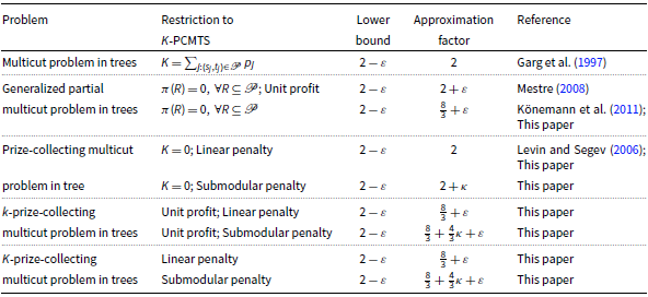
is any fixed positive number. Let us note that the algorithm presented in this paper improved the aforementioned two approximation factors. The k-prize-collecting restriction has been studied in combinatorial optimization and approximation algorithms, which can be found in Pedrosa and Rosado (Reference Pedrosa and Rosado2022), Liu et al. (Reference Liu, Li and Yang2022), Ren et al. (Reference Ren, Xu, Du and Li2022), and Liu and Li (Reference Liu and Li2023). The partial known results for the multicut problems in trees are given in Table 1.
$\varepsilon$
is any fixed positive number. Let us note that the algorithm presented in this paper improved the aforementioned two approximation factors. The k-prize-collecting restriction has been studied in combinatorial optimization and approximation algorithms, which can be found in Pedrosa and Rosado (Reference Pedrosa and Rosado2022), Liu et al. (Reference Liu, Li and Yang2022), Ren et al. (Reference Ren, Xu, Du and Li2022), and Liu and Li (Reference Liu and Li2023). The partial known results for the multicut problems in trees are given in Table 1.
Table 1. Results for the multicut problems in trees;
 $\kappa$
is the total curvature of the submodular penalty function
$\kappa$
is the total curvature of the submodular penalty function
1.2 Our results
In this paper, we present a combinatorial polynomial-time approximation for the K-PCMTS. In our approach, we utilize the primal algorithm for the multicut problem in trees with submodular functions in Liu and Li (Reference Liu and Li2022). One difficulty in implementing this primal-dual algorithm on the K-PCMTS is that the output solution is not feasible, i.e., the total profit of the disconnected pairs by the output solution is less than K. The reason is that the penalty for still-connected pairs is less than the cost of any edge that can disconnect them. Based on this observation, by carefully increasing the penalty of each pair, we can obtain a feasible solution for the K-PCMTS.
We show that the approximation factor of the proposed algorithm is
 $(\frac{8}{3}+\frac{4}{3}\kappa+ \varepsilon)$
, where
$(\frac{8}{3}+\frac{4}{3}\kappa+ \varepsilon)$
, where
 $\varepsilon$
is any fixed positive number and
$\varepsilon$
is any fixed positive number and
 $\kappa\leq 1$
is the total curvature of the nondecreasing submodular function (defined in (4)). When
$\kappa\leq 1$
is the total curvature of the nondecreasing submodular function (defined in (4)). When
 $\pi(R)=0$
for any
$\pi(R)=0$
for any
 $R\subseteq \mathcal{P}$
, the K-PCMTS is the generalized partial multicut problem in trees; then, our factor is
$R\subseteq \mathcal{P}$
, the K-PCMTS is the generalized partial multicut problem in trees; then, our factor is
 $\frac{8}{3}+\varepsilon$
, which coincides with the best-known ratio in Könemann et al. (Reference Könemann, Parekh and Segev2011).
$\frac{8}{3}+\varepsilon$
, which coincides with the best-known ratio in Könemann et al. (Reference Könemann, Parekh and Segev2011).
The remaining sections of this paper are organized as follows. In Section 2, we provide basic definitions and a formal problem statement. In Section 3, we consider the K-PCMTS. In Section 4, we conduct a simple simulation to evaluate the performance of the approximation algorithm. Finally, we provide a brief conclusion.
2. Preliminaries
Let
 $\mathcal{P}=\{(s_1,t_1),(s_2,t_2),\ldots, (s_m,t_m)\}$
be a given ground set and let
$\mathcal{P}=\{(s_1,t_1),(s_2,t_2),\ldots, (s_m,t_m)\}$
be a given ground set and let
 $\pi:2^{\mathcal{P}}\rightarrow \mathbf{R}$
be a real-valued function defined on all subsets of
$\pi:2^{\mathcal{P}}\rightarrow \mathbf{R}$
be a real-valued function defined on all subsets of
 $\mathcal{P}$
with
$\mathcal{P}$
with
 $\pi(\emptyset)=0$
. We assume that
$\pi(\emptyset)=0$
. We assume that
 $\pi(\!\cdot\!)$
is given as an evaluation oracle, which returns the value of
$\pi(\!\cdot\!)$
is given as an evaluation oracle, which returns the value of
 $\pi(R)$
for any
$\pi(R)$
for any
 $R\subseteq \mathcal{P}$
in polynomial time. If
$R\subseteq \mathcal{P}$
in polynomial time. If
 \begin{eqnarray}\pi( R_1) \leq \pi( R_2), ~\forall R_1 \subseteq R_2\subseteq \mathcal{P},\end{eqnarray}
function
 $\pi(\!\cdot\!)$
is called nondecreasing. If
$\pi(\!\cdot\!)$
is called nondecreasing. If
 \begin{eqnarray} \pi (R_1) +\pi (R_2)\geq \pi(R_1\cup R_2)+\pi (R_1\cap R_2) ,\forall R_1,R_2\subseteq \mathcal{P},\end{eqnarray}
the function
 $\pi(\!\cdot\!)$
is called submodular, which has the property of decreasing marginal return (Fujishige Reference Fujishige2005), i.e., for any
$\pi(\!\cdot\!)$
is called submodular, which has the property of decreasing marginal return (Fujishige Reference Fujishige2005), i.e., for any
 $ R_1\subseteq R_2 \subset \mathcal{P}$
and
$ R_1\subseteq R_2 \subset \mathcal{P}$
and
 $(s_j,t_j)\in \mathcal{P}\setminus R_2$
, we have
$(s_j,t_j)\in \mathcal{P}\setminus R_2$
, we have
 \begin{eqnarray} \pi((s_j,t_j)| R_1)\geq \pi((s_j,t_j)| R_2), \end{eqnarray}
where
 $\pi((s_j,t_j)|R)=\pi(R\cup \{(s_j,t_j)\})-\pi(R)$
for any
$\pi((s_j,t_j)|R)=\pi(R\cup \{(s_j,t_j)\})-\pi(R)$
for any
 $R\subseteq \mathcal{P}\setminus \{ (s_j,t_j) \}$
.
$R\subseteq \mathcal{P}\setminus \{ (s_j,t_j) \}$
.
As in Conforti and Cornuéjols (Reference Conforti and Cornuéjols1984), given a submodular function
 $\pi(\!\cdot\!)$
, the total curvature
$\pi(\!\cdot\!)$
, the total curvature
 $\kappa$
of
$\kappa$
of
 $\pi(\!\cdot\!)$
, which is the central concept in this paper, is defined as
$\pi(\!\cdot\!)$
, which is the central concept in this paper, is defined as
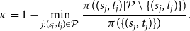 \begin{eqnarray} \kappa=1-\min_{j:(s_j,t_j)\in \mathcal{P}}\frac{\pi((s_j,t_j)|\mathcal{P}\setminus\{(s_j,t_j)\})}{\pi(\{(s_j,t_j)\})} . \end{eqnarray}
If
 $\pi(\!\cdot\!)$
is a nondecreasing submodular function, then for any
$\pi(\!\cdot\!)$
is a nondecreasing submodular function, then for any
 $\forall (s_j,t_j)\in \mathcal{P}$
, we have that
$\forall (s_j,t_j)\in \mathcal{P}$
, we have that
 $$ 0\leq \frac{\pi(\mathcal{P})-\pi(\mathcal{P}\setminus\{(s_j,t_j)\})}{\pi(\{(s_j,t_j)\})}= \frac{\pi((s_j,t_j)|\mathcal{P}\setminus\{(s_j,t_j)\})}{\pi(\{(s_j,t_j)\})}\leq \frac{\pi(\{(s_j,t_j)\}|\emptyset)}{\pi(\{(s_j,t_j)\})}= 1,$$
where the first inequality follows from inequality (1) and the second inequality follows from inequality (3). This implies that
 $$0\leq \kappa\leq 1, {\rm ~if~}\pi(\!\cdot\!){\rm~is~ a~ nondecreasing~ submodular~ function}.$$
In particular, if
 $$\pi(R)=\sum_{j:(s_j,t_j)\in R}\pi (\{(s_j,t_j)\}),~\forall R\subseteq \mathcal{P},$$
function
 $\pi(\!\cdot\!)$
is called linear, which implies that
$\pi(\!\cdot\!)$
is called linear, which implies that
 $$\kappa=1-\min_{j:(s_j,t_j)\in \mathcal{P}}\frac{\pi((s_j,t_j)|\mathcal{P}\setminus\{(s_j,t_j)\})}{\pi(\{(s_j,t_j)\})}=1-\min_{j:(s_j,t_j)\in \mathcal{P}}\frac{\pi(\{(s_j,t_j)\})}{\pi(\{(s_j,t_j)\})}=0.$$
We are given a tree
 $T=(V,E)$
with
$T=(V,E)$
with
 $V=\{v_1,v_2,\ldots,v_n\}$
and
$V=\{v_1,v_2,\ldots,v_n\}$
and
 $E=\{e_1,e_2,\ldots,e_{n-1}\}$
, a set
$E=\{e_1,e_2,\ldots,e_{n-1}\}$
, a set
 $\mathcal{P}=\{(s_1,t_1),(s_2,t_2),\ldots, (s_m,t_m)\}$
of m source–sink pairs of vertices with
$\mathcal{P}=\{(s_1,t_1),(s_2,t_2),\ldots, (s_m,t_m)\}$
of m source–sink pairs of vertices with
 $s_j,t_j\in V$
, a nondecreasing submodular penalty function
$s_j,t_j\in V$
, a nondecreasing submodular penalty function
 $\pi:2^{\mathcal{P}}\rightarrow \mathbf{R}_{\geq 0}$
, and a profit lower bound K. Each edge
$\pi:2^{\mathcal{P}}\rightarrow \mathbf{R}_{\geq 0}$
, and a profit lower bound K. Each edge
 $e\in E$
has a positive cost
$e\in E$
has a positive cost
 $c_e$
, and each source–sink pair
$c_e$
, and each source–sink pair
 $(s_j,t_j)\in \mathcal{P}$
can obtain a positive profit
$(s_j,t_j)\in \mathcal{P}$
can obtain a positive profit
 $p_j$
if
$p_j$
if
 $s_j$
and
$s_j$
and
 $t_j$
are disconnected by removing some edge set from T, i.e., for any
$t_j$
are disconnected by removing some edge set from T, i.e., for any
 $M\subseteq E$
, a pair
$M\subseteq E$
, a pair
 $(s_j,t_j)$
is disconnected by M if
$(s_j,t_j)$
is disconnected by M if
 $M\cap L_j \neq \emptyset$
, where
$M\cap L_j \neq \emptyset$
, where
 $L_j$
is the set of edges in the unique path from
$L_j$
is the set of edges in the unique path from
 $s_j$
to
$s_j$
to
 $t_j$
in tree T. Correspondingly, let
$t_j$
in tree T. Correspondingly, let
 $D_M$
be the set of pairs disconnected by M. The K-prize-collecting multicut problem in trees with submodular penalties (K-PCMTS) is to find a partial multicut
$D_M$
be the set of pairs disconnected by M. The K-prize-collecting multicut problem in trees with submodular penalties (K-PCMTS) is to find a partial multicut
 $M\subseteq E$
such that the total profit of the disconnected pairs by M is at least K, i.e.,
$M\subseteq E$
such that the total profit of the disconnected pairs by M is at least K, i.e.,
 $p(D_M)\geq K$
, and
$p(D_M)\geq K$
, and
 $c(M)+\pi(R_M)$
is minimized, where
$c(M)+\pi(R_M)$
is minimized, where
 $R_M=\mathcal{P}\setminus D_M$
is the set of pairs still connected after removing M. We define this setup as
$R_M=\mathcal{P}\setminus D_M$
is the set of pairs still connected after removing M. We define this setup as
 \begin{eqnarray*} c(M)=\sum_{e:e\in M} c_e,{\rm ~and~} p(D_M)=\sum_{j:(s_j,t_j)\in D_M} p_j,~\forall M\subseteq E. \end{eqnarray*}
For any
 $M\subseteq E$
, we obtain the set
$M\subseteq E$
, we obtain the set
 $R_M$
of pairs still connected after removing M, and we introduce binary variables
$R_M$
of pairs still connected after removing M, and we introduce binary variables
 $x_e,z_R$
, where
$x_e,z_R$
, where
 $x_e=1$
if and only if
$x_e=1$
if and only if
 $e\in M$
and
$e\in M$
and
 $z_R=1$
if and only if
$z_R=1$
if and only if
 $R=R_M$
. The K-PCMTS can be formulated as the following integer program:
$R=R_M$
. The K-PCMTS can be formulated as the following integer program:
 \begin{eqnarray} &~&\min \sum_{e:e\in E}c_e x_{e}+\sum_{R:R\subseteq \mathcal{P}} \pi(R) z_R\nonumber \\ \textit{s.t.} &~&\sum_{e:e\in L_j} x_e+\sum_{R\subseteq \mathcal{P}:(s_j,t_j)\in R}z_R \geq 1, ~ \forall (s_j,t_j)\in \mathcal{P} ,\\ &~&\sum_{R:R\in \mathcal{P}}\sum_{j:(s_j,t_j)\in R}p_j z_R\leq p({\mathcal{P}})-K,\nonumber\\ &~ & x_{e},z_R\in \{0,1\},~ \forall e\in E, ~ R\subseteq \mathcal{P}, \nonumber \end{eqnarray}
The first set of constraints ensures that each pair
 $(s_j,t_j)$
in
$(s_j,t_j)$
in
 $\mathcal{P}$
is either disconnected by an edge in
$\mathcal{P}$
is either disconnected by an edge in
 $L_j$
(the set of edges in the unique path from
$L_j$
(the set of edges in the unique path from
 $s_j$
to
$s_j$
to
 $t_j$
in tree T) or penalized, and the second constraint ensures that the total profit of the disconnected pairs is at least K.
$t_j$
in tree T) or penalized, and the second constraint ensures that the total profit of the disconnected pairs is at least K.
Lemma 1. Given an instance
 $\mathcal{I}=(V,E;\;\mathcal{P};\;K,\pi,c,p)$
for the K-PCMTS, for any
$\mathcal{I}=(V,E;\;\mathcal{P};\;K,\pi,c,p)$
for the K-PCMTS, for any
 $R\subset \mathcal{P}$
and
$R\subset \mathcal{P}$
and
 $(s_j,t_j)\in \mathcal{P} \setminus R$
, we have
$(s_j,t_j)\in \mathcal{P} \setminus R$
, we have
 \begin{eqnarray} 0\leq (1-\kappa)\cdot \pi(\{(s_j,t_j)\}) \leq \pi((s_j,t_j)|\mathcal{P}\setminus \{(s_j,t_j)\})\leq \pi((s_j,t_j)|R)\leq \pi(\{(s_j,t_j)\}). \end{eqnarray}
Proof. For any
 $R\subset \mathcal{P}$
and
$R\subset \mathcal{P}$
and
 $(s_j,t_j)\in \mathcal{P} \setminus R$
, we have
$(s_j,t_j)\in \mathcal{P} \setminus R$
, we have
 $$\pi((s_j,t_j)|\mathcal{P}\setminus \{(s_j,t_j)\})\leq \pi((s_j,t_j)|R)\leq \pi(\{(s_j,t_j)\}|\emptyset)=\pi(\{(s_j,t_j)\}),$$
where the inequalities follow from inequality (3).
Based on the above analysis, we have
 $0\leq \kappa \leq 1$
. If
$0\leq \kappa \leq 1$
. If
 $\kappa =1$
, for any
$\kappa =1$
, for any
 $(s_j,t_j)\in \mathcal{P}$
, we have that
$(s_j,t_j)\in \mathcal{P}$
, we have that
 $$\pi((s_j,t_j)|\mathcal{P}\setminus \{(s_j,t_j)\})=\pi(\mathcal{P})-\pi(\mathcal{P}\setminus \{(s_j,t_j)\})\geq0= (1-\kappa)\cdot \pi(\{(s_j,t_j)\}),$$
where the inequality follows from inequality (1). Otherwise,
 $0\leq \kappa < 1$
; for any
$0\leq \kappa < 1$
; for any
 $(s_j,t_j)\in \mathcal{P}$
, based on the definition of the total curvature in (4), it is not difficult to obtain that
$(s_j,t_j)\in \mathcal{P}$
, based on the definition of the total curvature in (4), it is not difficult to obtain that
 \begin{eqnarray*}\pi((s_j,t_j)|\mathcal{P}\setminus \{(s_j,t_j)\})>0, \;\;{\rm and}\;\; \kappa\geq 1- \frac{\pi((s_j,t_j)|\mathcal{P}\setminus\{(s_j,t_j)\})}{\pi(\{(s_j,t_j)\})}. \end{eqnarray*}
These findings imply that
 $$\pi((s_j,t_j)|\mathcal{P}\setminus\{(s_j,t_j)\})\geq (1-\kappa)\cdot \pi(\{(s_j,t_j)\})\geq (1-\kappa)\cdot \pi((s_j,t_j)|\mathcal{P}\setminus \{(s_j,t_j)\}) > 0, $$
where the second inequality follows from inequality (1).
Therefore, the lemma holds.
For convenience, let
 $\varepsilon$
be a given, fixed, positive number. Let
$\varepsilon$
be a given, fixed, positive number. Let
 $M^*$
be an optimal solution to the K-PCMTS with objective value OPT; let
$M^*$
be an optimal solution to the K-PCMTS with objective value OPT; let
 $R_{M^*}$
be the set of the pairs still connected after removing
$R_{M^*}$
be the set of the pairs still connected after removing
 $M^*$
. Inspired by the preprocessing step in Levin and Segev (Reference Levin and Segev2006), there are at most
$M^*$
. Inspired by the preprocessing step in Levin and Segev (Reference Levin and Segev2006), there are at most
 $\lfloor1/ \varepsilon \rfloor$
edges in
$\lfloor1/ \varepsilon \rfloor$
edges in
 $M^*$
with
$M^*$
with
 $c_e \geq \varepsilon \cdot OPT$
. Therefore, we can estimate all edges whose cost is greater than
$c_e \geq \varepsilon \cdot OPT$
. Therefore, we can estimate all edges whose cost is greater than
 $\varepsilon \cdot OPT$
in
$\varepsilon \cdot OPT$
in
 $M^*$
by evaluating all
$M^*$
by evaluating all
 $O(n^{\lfloor1/ \varepsilon \rfloor})$
subsets
$O(n^{\lfloor1/ \varepsilon \rfloor})$
subsets
 $H\subseteq E$
with a cardinality of at most
$H\subseteq E$
with a cardinality of at most
 $\lfloor1/ \varepsilon \rfloor$
. We include H in the solution, eliminate the subset of pairs separated by H, update the requirement parameter, and contract all edges whose cost is greater than
$\lfloor1/ \varepsilon \rfloor$
. We include H in the solution, eliminate the subset of pairs separated by H, update the requirement parameter, and contract all edges whose cost is greater than
 $\min_{e:e\in H}c_e$
. Thus,we assume that any edge,
$\min_{e:e\in H}c_e$
. Thus,we assume that any edge,
 $e\in E$
, satisfies
$e\in E$
, satisfies
 \begin{eqnarray} c_e\leq \varepsilon\cdot OPT.\end{eqnarray}
3. The K-PCMTS
The K-PCMTS is an extension of the multicut problem in trees with submodular penalties (MTS) and has a primal-dual 3-approximation algorithm (Liu and Li Reference Liu and Li2022) denoted as
 $\mathcal{A}$
. However, the output solution to
$\mathcal{A}$
. However, the output solution to
 $\mathcal{A}$
may not be a feasible solution to the K-PCMTS since the total profit of disconnected pairs is less than K. Extending the algorithm presented in Levin and Segev (Reference Levin and Segev2006), we present an algorithm for the K-PCMTS by utilizing the primal-dual algorithm
$\mathcal{A}$
may not be a feasible solution to the K-PCMTS since the total profit of disconnected pairs is less than K. Extending the algorithm presented in Levin and Segev (Reference Levin and Segev2006), we present an algorithm for the K-PCMTS by utilizing the primal-dual algorithm
 $\mathcal{A}$
on the instance of the MTS with an increasing penalty.
$\mathcal{A}$
on the instance of the MTS with an increasing penalty.
In Subsection 3.1, we first define the instance of the MTS with the increasing penalty. Then, we recall the primal-dual algorithm
 $\mathcal{A}$
(Liu and Li Reference Liu and Li2022), and we introduce some key lemmas. In Subsection 3.2, we present a polynomial-time approximation algorithm for the K-PCMTS, and we prove that the objective of its output solution M is
$\mathcal{A}$
(Liu and Li Reference Liu and Li2022), and we introduce some key lemmas. In Subsection 3.2, we present a polynomial-time approximation algorithm for the K-PCMTS, and we prove that the objective of its output solution M is
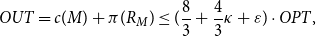 $$OUT=c(M)+\pi(R_M)\leq (\frac{8}{3}+\frac{4}{3}\kappa+ \varepsilon)\cdot OPT,$$
where OPT denotes the optimal value for the K-PCMTS.
3.1 Instance of the MTS with increasing penalty and the primal-dual algorithm
Given an instance
 $\mathcal{I}=(V,E;\;\mathcal{P};\;K,\pi,c,p)$
for the K-PCMTS, for any
$\mathcal{I}=(V,E;\;\mathcal{P};\;K,\pi,c,p)$
for the K-PCMTS, for any
 $\lambda\geq 0$
, we construct an instance
$\lambda\geq 0$
, we construct an instance
 $\mathcal{I}_{\lambda}=(V,E;\;\mathcal{P};\;\pi_{\lambda},c)$
of the MTS with an increasing penalty for
$\mathcal{I}_{\lambda}=(V,E;\;\mathcal{P};\;\pi_{\lambda},c)$
of the MTS with an increasing penalty for
 $\lambda$
, where
$\lambda$
, where
 $\pi_\lambda(\!\cdot\!)$
is defined as follows:
$\pi_\lambda(\!\cdot\!)$
is defined as follows:
 \begin{eqnarray} \pi_{\lambda}(R)=\pi(R)+\sum_{j:(s_j,t_j)\in R}\lambda\cdot p_j=\pi(R)+\lambda\cdot p(R),~\forall R\subseteq \mathcal{P}.\end{eqnarray}
The MTS represents the multicut problem with a submodular penalty, in which the objective is to find a multicut
 $M_{\lambda}\subseteq E$
such that the total cost of edges in
$M_{\lambda}\subseteq E$
such that the total cost of edges in
 $M_{\lambda}$
plus the penalty of the set of pairs still connected after removing
$M_{\lambda}$
plus the penalty of the set of pairs still connected after removing
 $M_{\lambda}$
is minimized, i.e.,
$M_{\lambda}$
is minimized, i.e.,
 $M_{\lambda}=\arg\min_{M:M\subseteq E}c(M)+\pi_{\lambda}(R_M)$
.
$M_{\lambda}=\arg\min_{M:M\subseteq E}c(M)+\pi_{\lambda}(R_M)$
.
Since function
 $\pi_{\lambda}(\!\cdot\!)$
is the sum of a nondecreasing submodular function
$\pi_{\lambda}(\!\cdot\!)$
is the sum of a nondecreasing submodular function
 $\pi(\!\cdot\!)$
and a linear function
$\pi(\!\cdot\!)$
and a linear function
 $p(\!\cdot\!)$
, the following lemma is easy to verify:
$p(\!\cdot\!)$
, the following lemma is easy to verify:
Lemma 2. (Fujishige Reference Fujishige2005)
 $\pi_{\lambda}(\!\cdot\!)$
is a nondecreasing submodular function.
$\pi_{\lambda}(\!\cdot\!)$
is a nondecreasing submodular function.
Then, the MTS for
 $\mathcal{I}_{\lambda}$
can be formulated as an integer program by
$\mathcal{I}_{\lambda}$
can be formulated as an integer program by
 \begin{eqnarray} &~&\min \sum_{e:e\in E}c_e x_{e}+\sum_{R:R\subseteq \mathcal{P}} \pi_{\lambda}(R) z_R\nonumber \\ \textit{s.t.} &~&\sum_{e:e\in L_j} x_e+\sum_{R\subseteq \mathcal{P}:(s_j,t_j)\in R}z_R \geq 1, ~ \forall (s_j,t_j)\in \mathcal{P} ,\\ &~ & x_{e},{z_R}\in \{0,1\},~ \forall e\in E, ~ R\subseteq \mathcal{P}, \nonumber\end{eqnarray}
where
 $L_j$
is the set of edges in the unique path from
$L_j$
is the set of edges in the unique path from
 $s_j$
to
$s_j$
to
 $t_j$
in tree T,
$t_j$
in tree T,
 $x_e$
indicates whether edge e is selected for the multicut, and
$x_e$
indicates whether edge e is selected for the multicut, and
 $z_R$
indicates whether R is selected to be rejected. The first set of constraints of (9) guarantees that each pair
$z_R$
indicates whether R is selected to be rejected. The first set of constraints of (9) guarantees that each pair
 $(s_j,t_j)\in \mathcal{P}$
is either disconnected by an edge in
$(s_j,t_j)\in \mathcal{P}$
is either disconnected by an edge in
 $L_j$
or penalized. Relaxing the integral constraints, we obtain a linear program where we need not add constraints
$L_j$
or penalized. Relaxing the integral constraints, we obtain a linear program where we need not add constraints
 $x_{e}\leq 1$
and
$x_{e}\leq 1$
and
 $z_R\leq 1$
since they are automatically satisfied in an optimal solution. The dual of this linear program is
$z_R\leq 1$
since they are automatically satisfied in an optimal solution. The dual of this linear program is
 \begin{eqnarray} &~&\max \sum_{j:(s_j,t_j)\in \mathcal{P}} y_j\nonumber \\ \textit{s.t.} &~&\sum_{j:e\in L_j} y_j \leq c_e, ~ \forall e\in E ,\\ &~&\sum_{j:(s_j,t_j)\in R}y_j \leq \pi_{\lambda}(R), ~ \forall R\subseteq \mathcal{P} ,\nonumber\\ &~ & y_j\geq 0, ~ \forall (s_j,t_j)\in \mathcal{P}. \nonumber\end{eqnarray}
Then, we recall algorithm
 $\mathcal{A}$
(Liu and Li Reference Liu and Li2022) based on the primal-dual scheme designed in Garg et al. (Reference Garg, Vazirani and Yannakakis1997).
$\mathcal{A}$
(Liu and Li Reference Liu and Li2022) based on the primal-dual scheme designed in Garg et al. (Reference Garg, Vazirani and Yannakakis1997).
Given an instance
 $\mathcal{I}_{\lambda}$
of the MTS, we consider a dual feasible solution
$\mathcal{I}_{\lambda}$
of the MTS, we consider a dual feasible solution
 $\mathbf{y}=(y_1,y_2,\ldots, y_{m})$
of (10), where entry
$\mathbf{y}=(y_1,y_2,\ldots, y_{m})$
of (10), where entry
 $y_j$
is a nonnegative variable for pair
$y_j$
is a nonnegative variable for pair
 $(s_j,t_j)\in \mathcal{P}$
. If
$(s_j,t_j)\in \mathcal{P}$
. If
 $\sum_{j:e\in L_j}y_j=c_e$
for any
$\sum_{j:e\in L_j}y_j=c_e$
for any
 $e\in E$
, then edge e is considered tight. Similarly, if
$e\in E$
, then edge e is considered tight. Similarly, if
 $\sum_{j:(s_j,t_j)\in R}y_j= \pi_{\lambda}(R)$
for any
$\sum_{j:(s_j,t_j)\in R}y_j= \pi_{\lambda}(R)$
for any
 $R\subseteq \mathcal{P}$
, then the pair set R is considered tight.
$R\subseteq \mathcal{P}$
, then the pair set R is considered tight.
Algorithm
 $\mathcal{A}$
designates r as the root, where r is an arbitrary vertex in the tree. Then, the level of a vertex is defined as its distance from root r, and the level of an edge
$\mathcal{A}$
designates r as the root, where r is an arbitrary vertex in the tree. Then, the level of a vertex is defined as its distance from root r, and the level of an edge
 $e = (u, v)$
is determined by the minimum level of vertices u and v. The root r is considered to be level 0. For each source–sink pair
$e = (u, v)$
is determined by the minimum level of vertices u and v. The root r is considered to be level 0. For each source–sink pair
 $(s_j,t_j)$
in
$(s_j,t_j)$
in
 $\mathcal{P}$
, we say that it is contained in subtree
$\mathcal{P}$
, we say that it is contained in subtree
 $T_v$
rooted at vertex v if the corresponding path
$T_v$
rooted at vertex v if the corresponding path
 $L_j$
lies entirely within this subtree. Additionally, a pair
$L_j$
lies entirely within this subtree. Additionally, a pair
 $(s_j,t_j)$
is considered contained in level l if it is contained within a subtree rooted at a vertex in level l. Let
$(s_j,t_j)$
is considered contained in level l if it is contained within a subtree rooted at a vertex in level l. Let
 $l_{max}$
be the maximum level that contains at least one pair in
$l_{max}$
be the maximum level that contains at least one pair in
 $\mathcal{P}$
. An edge
$\mathcal{P}$
. An edge
 $e_1$
is an ancestor of an edge
$e_1$
is an ancestor of an edge
 $e_2$
if
$e_2$
if
 $e_1$
lies on the path from
$e_1$
lies on the path from
 $e_2$
to the root.
$e_2$
to the root.
In the algorithm,
 $\mathcal{P}^{disc}$
denotes the set of pairs that are disconnected after removing the selected edges;
$\mathcal{P}^{disc}$
denotes the set of pairs that are disconnected after removing the selected edges;
 $R^{temp}$
denotes the set of pairs that are tight and temporarily rejected.
$R^{temp}$
denotes the set of pairs that are tight and temporarily rejected.
Initially, we set
 $\mathbf{y}=\mathbf{0}$
and
$\mathbf{y}=\mathbf{0}$
and
 $M_{\lambda}=R_{M_{\lambda}}=\mathcal{P}^{disc}=R^{temp}=\emptyset$
. The algorithm consists of two phases over the tree.
$M_{\lambda}=R_{M_{\lambda}}=\mathcal{P}^{disc}=R^{temp}=\emptyset$
. The algorithm consists of two phases over the tree.
Phase 1. The algorithm moves the tree from level
 $l_{max}$
to level 0, one level at a time, adding some edges to M. At each level
$l_{max}$
to level 0, one level at a time, adding some edges to M. At each level
 $l= l_{max}, l_{max}-1, \ldots , 0$
, for every vertex v in level l such that
$l= l_{max}, l_{max}-1, \ldots , 0$
, for every vertex v in level l such that
 $T_v$
contains at least one pair in
$T_v$
contains at least one pair in
 $\mathcal{P}\setminus(\mathcal{P}^{disc}\cup R^{temp})$
. Let
$\mathcal{P}\setminus(\mathcal{P}^{disc}\cup R^{temp})$
. Let
 $\mathcal{P}_v$
contain all the pairs of
$\mathcal{P}_v$
contain all the pairs of
 $\mathcal{P}\setminus(\mathcal{P}^{disc}\cup R^{temp})$
in subtree
$\mathcal{P}\setminus(\mathcal{P}^{disc}\cup R^{temp})$
in subtree
 $T_v$
. For each pair
$T_v$
. For each pair
 $(s_j,t_j)\in \mathcal{P}_v$
, the algorithm increases the dual variable
$(s_j,t_j)\in \mathcal{P}_v$
, the algorithm increases the dual variable
 $y_j$
as much as possible until either an edge or a pair set becomes tight.
$y_j$
as much as possible until either an edge or a pair set becomes tight.
Case 1. If there is an edge
 $e\in L_j$
that becomes tight, then the algorithm adds
$e\in L_j$
that becomes tight, then the algorithm adds
 $(s_j,t_j)$
to
$(s_j,t_j)$
to
 $\mathcal{P}^{disc}$
. All tight edges are added to the set of the frontier(v), which is the frontier of vertex v. If there are two edges in the frontier(v) such that one edge is an ancestor of the other edge, then we need only the ancestor in the set of frontier(v).
$\mathcal{P}^{disc}$
. All tight edges are added to the set of the frontier(v), which is the frontier of vertex v. If there are two edges in the frontier(v) such that one edge is an ancestor of the other edge, then we need only the ancestor in the set of frontier(v).
Case 2. If there is a subset
 $R\subseteq \mathcal{P}$
that becomes tight, then the algorithm adds all the pairs in R to temporary set
$R\subseteq \mathcal{P}$
that becomes tight, then the algorithm adds all the pairs in R to temporary set
 $R^{temp}$
.
$R^{temp}$
.
Phase 2. The algorithm moves down the tree one level at a time from level 0 to level
 $l_{max}$
and builds the final output solution to
$l_{max}$
and builds the final output solution to
 $M_{\lambda}$
. At each level
$M_{\lambda}$
. At each level
 $l=0,1,\ldots, l_{max}$
, for every vertex v in level l, such that frontier(v)
$l=0,1,\ldots, l_{max}$
, for every vertex v in level l, such that frontier(v)
 $\neq \emptyset$
, and the algorithm considers the edges in frontier(v). For each edge
$\neq \emptyset$
, and the algorithm considers the edges in frontier(v). For each edge
 $e\in\;$
frontier(v), if no edge along the path from e to v is already included in
$e\in\;$
frontier(v), if no edge along the path from e to v is already included in
 $M_{\lambda}$
; then, the algorithm adds e to
$M_{\lambda}$
; then, the algorithm adds e to
 $M_{\lambda}$
. Finally, for each pair
$M_{\lambda}$
. Finally, for each pair
 $(s_j,t_j)\in R^{temp}$
, if there is no edge
$(s_j,t_j)\in R^{temp}$
, if there is no edge
 $e\in M_{\lambda} \cap L_j$
, then
$e\in M_{\lambda} \cap L_j$
, then
 $(s_j,t_j)$
is added to
$(s_j,t_j)$
is added to
 $R_{M_{\lambda}}$
.
$R_{M_{\lambda}}$
.
Let
 $\mathbf{y}$
be the vector generated by
$\mathbf{y}$
be the vector generated by
 $\mathcal{A}$
. The following lemmas are easy to obtain by Lemma 2 and (Garg et al. Reference Garg, Vazirani and Yannakakis1997; Liu and Li Reference Liu and Li2022).
$\mathcal{A}$
. The following lemmas are easy to obtain by Lemma 2 and (Garg et al. Reference Garg, Vazirani and Yannakakis1997; Liu and Li Reference Liu and Li2022).
Lemma 3. (Liu and Li Reference Liu and Li2022)
 $\mathbf{y}$
is a feasible solution to the dual program (10), and
$\mathbf{y}$
is a feasible solution to the dual program (10), and
 $\mathcal{A}$
can be implemented in
$\mathcal{A}$
can be implemented in
 $O(n^{6}\cdot \rho+n^{7})$
, where
$O(n^{6}\cdot \rho+n^{7})$
, where
 $\rho$
is the running time of evaluating (the oracle for)
$\rho$
is the running time of evaluating (the oracle for)
 $\pi$
.
$\pi$
.
Proof. In any iteration, the tight set in Case 2 can be found in
 $O(n^{5}\cdot \rho+n^{6})$
by using the combinatorial algorithm for the submodular minimization problem (Orlin Reference Orlin2009). Since at least one pair is added to either
$O(n^{5}\cdot \rho+n^{6})$
by using the combinatorial algorithm for the submodular minimization problem (Orlin Reference Orlin2009). Since at least one pair is added to either
 $\mathcal{P}^{disc}$
or
$\mathcal{P}^{disc}$
or
 $R^{temp}$
in any iteration of Phase 1, it is easy to determine that Algorithm 3.2 can be implemented in
$R^{temp}$
in any iteration of Phase 1, it is easy to determine that Algorithm 3.2 can be implemented in
 $O(n^{6}\cdot \rho+n^{7})$
.
$O(n^{6}\cdot \rho+n^{7})$
.
Lemma 4.
 $\pi_{\lambda}((s_j,t_j)|\mathcal{P}\setminus\{(s_j,t_j)\})\leq y_j\leq \pi_{\lambda}(\{(s_j,t_j)\}),~\forall (s_j,t_j)\in R^{temp}$
Proof. Based on Lemma 3, we have
 $\sum_{j:(s_j,t_j)\in R}y_j\leq \pi_{\lambda}(R)$
for any set
$\sum_{j:(s_j,t_j)\in R}y_j\leq \pi_{\lambda}(R)$
for any set
 $R\subseteq \mathcal{P}$
by the second set of constraints of (10). This implies that
$R\subseteq \mathcal{P}$
by the second set of constraints of (10). This implies that
 $$y_j\leq \pi_{\lambda}(\{(s_j,t_j)\}),\forall (s_j,t_j)\in R^{temp}.$$
For any pair
 $(s_j,t_j)\in R^{temp}$
, by Case 2 of
$(s_j,t_j)\in R^{temp}$
, by Case 2 of
 $\mathcal{A}$
, there exists a tight set R with
$\mathcal{A}$
, there exists a tight set R with
 $(s_j,t_j)\in R$
, i.e.,
$(s_j,t_j)\in R$
, i.e.,
 $$\pi_{\lambda}(R)=\sum_{j:(s_j,t_j)\in R}y_j=y_j+\sum_{j':(s_{j'},t_{j'})\in R\setminus\{(s_j,t_j)\}}y_{j'}\leq y_j+ \pi_{\lambda}(R\setminus\{(s_j,t_j)\}) .$$
Rearranging the above inequality, for any pair
 $(s_j,t_j)\in R^{temp}$
, we have
$(s_j,t_j)\in R^{temp}$
, we have
 $$y_j\geq \pi_{\lambda}(R)-\pi_{\lambda}(R\setminus\{(s_j,t_j)\})=\pi_{\lambda}((s_j,t_j)| R\setminus\{(s_j,t_j)\})\geq \pi_{\lambda}((s_j,t_j)|\mathcal{P}\setminus\{(s_j,t_j)\}),$$
where the last inequality follows from Lemma 2 and inequality (3).
Lemma 5. (Liu and Li Reference Liu and Li2022)
 $\pi_{\lambda}(R^{temp})=\sum_{j:(s_j,t_j)\in R^{temp}}y_j.$
Lemma 6. (Garg et al. Reference Garg, Vazirani and Yannakakis1997) For any
 $(s_j,t_j)\in \mathcal{P}$
with
$(s_j,t_j)\in \mathcal{P}$
with
 $y_j>0$
,
$y_j>0$
,
 $M_{\lambda}$
generated by
$M_{\lambda}$
generated by
 $\mathcal{A}$
satisfies
$\mathcal{A}$
satisfies
 $|M_{\lambda}\cap L_j| \leq 2$
.
$|M_{\lambda}\cap L_j| \leq 2$
.
Lemma 7. Let
 $\kappa_{\lambda}$
be the total curvature of
$\kappa_{\lambda}$
be the total curvature of
 $\pi_{\lambda}$
; then,
$\pi_{\lambda}$
; then,
 $M_{\lambda}$
generated by
$M_{\lambda}$
generated by
 $\mathcal{A}$
satisfies
$\mathcal{A}$
satisfies
 $$\sum_{e:e\in M_{\lambda}}c_e+ \pi_{\lambda}(R_{M_{\lambda}})+(1+\kappa_{\lambda})\cdot\sum_{e:e\in R_{M_{\lambda}}}\pi_{\lambda}(\{(s_j,t_j)\}|\mathcal{P}\setminus \{(s_j,t_j)\})\leq (2+\kappa_{\lambda})\cdot OPT_{\lambda},$$
where
 $OPT_{\lambda}$
denotes the optimal value for instance
$OPT_{\lambda}$
denotes the optimal value for instance
 $\mathcal{I}_{\lambda}$
, of the MTS.
$\mathcal{I}_{\lambda}$
, of the MTS.
Proof. For any edge
 $e\in M_{\lambda}$
, e is a tight edge, i.e.,
$e\in M_{\lambda}$
, e is a tight edge, i.e.,
 $\sum_{j:e\in L_j }y_j = c_e$
. The objective value of
$\sum_{j:e\in L_j }y_j = c_e$
. The objective value of
 $M_{\lambda}$
is
$M_{\lambda}$
is
 \begin{eqnarray*} && \sum_{e:e\in M_{\lambda}}c_e+ \pi_{\lambda}(R_{M_{\lambda}})\\ &= & \sum_{e:e\in M_{\lambda}}\sum_{j:e\in L_j}y_j+\pi_{\lambda}(R^{temp})-\pi_{\lambda}(R^{temp})+\pi_{\lambda}(R_{M_{\lambda}})\\ &= & \sum_{j:(s_j,t_j)\in D_{M_{\lambda}}}y_j\cdot |M_{\lambda}\cap L_j|+\sum_{j:(s_j,t_j)\in R^{temp}}y_j-\pi_{\lambda}(R^{temp})+\pi_{\lambda}(R_{M_{\lambda}})\\ &\leq& 2 \cdot\sum_{j:(s_j,t_j)\in D_{M_{\lambda}}}y_j+\sum_{j:(s_j,t_j)\in R^{temp}}y_j-\sum_{j:(s_j,t_j)\in R^{temp}\setminus R_{M_{\lambda}} }\pi_{\lambda}((s_j,t_j)|\mathcal{P}\setminus\{(s_j,t_j)\} )\\ &\leq& 2 \cdot\sum_{j:(s_j,t_j)\in D_{M_{\lambda}}}y_j+\sum_{j:(s_j,t_j)\in R^{temp}}y_j-\sum_{j:(s_j,t_j)\in R^{temp}\setminus R_{M_{\lambda}} }(1-\kappa_{\lambda})\cdot\pi_{\lambda}(\{(s_j,t_j)\})\\ &\leq& 2 \cdot\sum_{j:(s_j,t_j)\in D_{M_{\lambda}}}y_j+\sum_{j:(s_j,t_j)\in R^{temp}}y_j-\sum_{j:(s_j,t_j)\in R^{temp}\setminus R_{M_{\lambda}} }(1-\kappa_{\lambda})\cdot y_j\\ &=& 2 \cdot\sum_{j:(s_j,t_j)\in D_{M_{\lambda}}}y_j+\kappa_{\lambda}\cdot \sum_{j:(s_j,t_j)\in R^{temp}}y_j+(1-\kappa_{\lambda})\cdot\sum_{j:(s_j,t_j)\in R_{M_{\lambda}}}y_j\\ &\leq& 2 \cdot\sum_{j:(s_j,t_j)\in D_{M_{\lambda}}}y_j+\kappa_{\lambda}\cdot (\sum_{j:(s_j,t_j)\in D_{M_\lambda}}y_j+\sum_{j:(s_j,t_j)\in R_{M_\lambda}}y_j)+(1-\kappa_{\lambda})\cdot\sum_{j:(s_j,t_j)\in R_{M_{\lambda}}}y_j\\ &=& (2+\kappa_{\lambda})\cdot\sum_{j:(s_j,t_j)\in \mathcal{P}}y_j-(1+\kappa_{\lambda})\cdot\sum_{j:(s_j,t_j)\in R_{M_{\lambda}}}y_j\\ &\leq& (2+\kappa_{\lambda})\cdot OPT_{\lambda}-(1+\kappa_{\lambda})\cdot\sum_{j:(s_j,t_j)\in R_{M_{\lambda}}}\pi_{\lambda}((s_j,t_j)|\mathcal{P}\setminus\{(s_j,t_j)\}), \end{eqnarray*}
where
 $D_{M_{\lambda}}$
is the set of pairs disconnected by
$D_{M_{\lambda}}$
is the set of pairs disconnected by
 ${M_{\lambda}}$
. The first and second inequalities follow from inequality (6) and Lemma 6, the third inequality follows from Lemma 4, the fourth inequality follows from
${M_{\lambda}}$
. The first and second inequalities follow from inequality (6) and Lemma 6, the third inequality follows from Lemma 4, the fourth inequality follows from
 $R^{temp}\subseteq \mathcal{P}=D_{M_{\lambda}}\cup R_{M_{\lambda}}$
, and the last inequality follows from Lemmas 3 and 4.
$R^{temp}\subseteq \mathcal{P}=D_{M_{\lambda}}\cup R_{M_{\lambda}}$
, and the last inequality follows from Lemmas 3 and 4.
Based on Lemma 7, when
 $\pi_{\lambda}(\!\cdot\!)$
is a linear function, i.e.,
$\pi_{\lambda}(\!\cdot\!)$
is a linear function, i.e.,
 $\kappa_{\lambda}=0$
, the approximation factor of
$\kappa_{\lambda}=0$
, the approximation factor of
 $\mathcal{A}$
is 2, which is equal to the approximation factor in Levin and Segev (Reference Levin and Segev2006); when
$\mathcal{A}$
is 2, which is equal to the approximation factor in Levin and Segev (Reference Levin and Segev2006); when
 $\pi_{\lambda}(\!\cdot\!)$
is a nondecreasing submodular function, we have that
$\pi_{\lambda}(\!\cdot\!)$
is a nondecreasing submodular function, we have that
 $\kappa_{\lambda}\leq 1$
, and the approximation factor of
$\kappa_{\lambda}\leq 1$
, and the approximation factor of
 $\mathcal{A}$
is no more than 3, where 3 is the approximation factor in Liu and Li (Reference Liu and Li2022). Thus, Lemma 7 provides a specific relationship between the approximation factor achieved by the algorithm and the total curvature of the penalty function. This relationship serves as a key component to derive the approximation factor of the following algorithm for the K-PCMTS problem.
$\mathcal{A}$
is no more than 3, where 3 is the approximation factor in Liu and Li (Reference Liu and Li2022). Thus, Lemma 7 provides a specific relationship between the approximation factor achieved by the algorithm and the total curvature of the penalty function. This relationship serves as a key component to derive the approximation factor of the following algorithm for the K-PCMTS problem.
3.2 Approximation algorithm for the K-PCMTS
For any
 $\lambda\geq 0$
, let
$\lambda\geq 0$
, let
 $M_{\lambda}$
denote the solution generated by
$M_{\lambda}$
denote the solution generated by
 $\mathcal{A}$
for instance
$\mathcal{A}$
for instance
 $\mathcal{I}_{\lambda}$
of the MTS with an increasing penalty for
$\mathcal{I}_{\lambda}$
of the MTS with an increasing penalty for
 $\lambda$
. Furthermore, let
$\lambda$
. Furthermore, let
 $p_{\lambda}$
be the total profit of the disconnected pairs obtained by removing
$p_{\lambda}$
be the total profit of the disconnected pairs obtained by removing
 $M_{\lambda}$
, i.e.,
$M_{\lambda}$
, i.e.,
 $$p_{\lambda} =p(D_{M_{\lambda}} ),$$
where
 $D_{M_{\lambda}}$
represents the set of pairs that become disconnected after removing
$D_{M_{\lambda}}$
represents the set of pairs that become disconnected after removing
 $M_{\lambda}$
.
$M_{\lambda}$
.
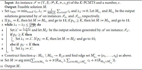
We present the algorithm for the K-PCMTS as follows:
(1) If the total profit of the disconnected pairs
 $p_{0}$
is greater than or equal to K, then the algorithm outputs solution
$M_0$
, and the algorithm is terminated.
$p_{0}$
is greater than or equal to K, then the algorithm outputs solution
$M_0$
, and the algorithm is terminated.(2) The algorithm conducts a binary search over the interval
$[0, \frac{1}{\min_{j}p_j}\sum_{e:e\in E}c_e+1]$
by using algorithm
$\mathcal{A}$
to find two values of
$\lambda$
, namely,
$\lambda_1$
and
$\lambda_2$
, which satisfy the following conditions: Here,
\begin{eqnarray*} \left\{ \begin{split} &\lambda_1> \lambda_2 ;\\ &\lambda_1- \lambda_2 \leq \frac{\varepsilon c_{min}}{p(\mathcal{P})};\\ &p_{\lambda_1}\geq K > p_{\lambda_2}. \end{split}\right.\end{eqnarray*}
$c_{min}$
represents the minimum cost among all edges in E, and
$p(\mathcal{P})=\sum_{j:(s_j,t_j)\in \mathcal{P}}p_j$
is the total profit of the source–sink pairs in
$\mathcal{P}$
. In particular, if there exists some
$\lambda$
satisfying
$p_{\lambda}=K$
, then the algorithm outputs solution
$M_{\lambda}$
and terminates.
(3) For each pair
$(s_j,t_j)\in D_{M_{\lambda_1}}\setminus D_{M_{\lambda_2}}$
, the algorithm assigns it to an arbitrary edge
$e\in M_{\lambda_1}\setminus M_{\lambda_2}$
with
$e\in L_j$
, where
$L_j$
is the set of edges in the unique path from
$s_j$
to
$t_j$
in tree T. Let
$\varphi(e)$
denote the total profit of pairs assigned to e. The algorithm sorts the edges in
$M_{\lambda_1}\setminus M_{\lambda_2}$
with
$\varphi(e)>0$
in nondecreasing order, i.e., (11)where
\begin{eqnarray}\frac{c_{e_1}}{\varphi(e_1)}\leq \frac{c_{e_2}}{\varphi(e_2)}\leq\cdots\leq \frac{c_{e_k}}{\varphi(e_k)},\end{eqnarray}
$k=\big|\{e\in M_{\lambda_1}\setminus M_{\lambda_2}|\varphi(e)>0\}\big|$
. Let
$M'_{\lambda_1}=\{e_1,\ldots,e_q\}$
be the first q edge in
$M_{\lambda_1}\setminus M_{\lambda_2}$
, where q is the minimal index satisfying
$\sum_{i=1}^q \varphi(e_i)\geq K- p_{\lambda_2}$
.
(4) The solution that minimizes the objective value between
$M_{\lambda_1}$
and
$M_{\lambda_2}\cup M'_{\lambda_1}$
is output, and the algorithm terminates. We propose the detailed primal-dual algorithm, which is shown in Algorithm 1:


Algorithm 1: Increasing penalty algorithm
Lemma 8.
 $\sum_{e\in M'_{\lambda_1}}c_e\leq \frac{K-p_{\lambda_2}}{{p_{\lambda_1} -p_{\lambda_2}}} \sum_{e:e\in M_{\lambda_1}\setminus M_{\lambda_2}}c_e+\varepsilon\cdot OPT$
.
$\sum_{e\in M'_{\lambda_1}}c_e\leq \frac{K-p_{\lambda_2}}{{p_{\lambda_1} -p_{\lambda_2}}} \sum_{e:e\in M_{\lambda_1}\setminus M_{\lambda_2}}c_e+\varepsilon\cdot OPT$
.
Proof. Since inequality (11) and
 $q\leq k$
, we have
$q\leq k$
, we have
 $\frac{ \sum_{i=1}^{q-1}c_{e_i}}{\sum_{i=1}^{q-1}\varphi(e_{i})} \leq \frac{ \sum_{i'=1}^{k}c_{e_{i'}}}{\sum_{i'=1}^k\varphi(e_{i'})} $
. Rearranging this inequality, we have
$\frac{ \sum_{i=1}^{q-1}c_{e_i}}{\sum_{i=1}^{q-1}\varphi(e_{i})} \leq \frac{ \sum_{i'=1}^{k}c_{e_{i'}}}{\sum_{i'=1}^k\varphi(e_{i'})} $
. Rearranging this inequality, we have
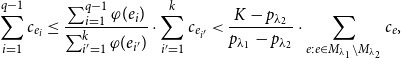 $$ \sum_{i=1}^{q-1}c_{e_i} \leq \frac{ \sum_{i=1}^{q-1}\varphi(e_i)}{\sum_{i'=1}^k\varphi(e_{i'})}\cdot \sum_{i'=1}^{k}c_{e_{i'}} < \frac{K-p_{\lambda_2}}{{p_{\lambda_1} -p_{\lambda_2}}} \cdot \sum_{e:e\in M_{\lambda_1}\setminus M_{\lambda_2}}c_e,$$
where the second inequality follows from
 $\sum_{i=1}^{q-1} \varphi(e_i)<\sum_{i=1}^{k} \varphi(e_i) =K- p_{\lambda_2}$
and
$\sum_{i=1}^{q-1} \varphi(e_i)<\sum_{i=1}^{k} \varphi(e_i) =K- p_{\lambda_2}$
and
 $\{e_1,\ldots,e_k\}\subseteq M_{\lambda_1}\setminus M_{\lambda_2}$
. Thus,
$\{e_1,\ldots,e_k\}\subseteq M_{\lambda_1}\setminus M_{\lambda_2}$
. Thus,
 $\sum_{i=1}^{q}c_{e_i} =\sum_{i=1}^{q-1}c_{e_i} +c_{e_q}< \frac{K-p_{\lambda_2}}{{p_{\lambda_1} -p_{\lambda_2}}} \sum_{e:e\in M_{\lambda_1}\setminus M_{\lambda_2}}c_e+\varepsilon\cdot OPT,$
where the inequality follows from inequality (7).
$\sum_{i=1}^{q}c_{e_i} =\sum_{i=1}^{q-1}c_{e_i} +c_{e_q}< \frac{K-p_{\lambda_2}}{{p_{\lambda_1} -p_{\lambda_2}}} \sum_{e:e\in M_{\lambda_1}\setminus M_{\lambda_2}}c_e+\varepsilon\cdot OPT,$
where the inequality follows from inequality (7).
Lemma 9. For any
 $\lambda\geq 0$
, let
$\lambda\geq 0$
, let
 $M_{\lambda}$
be the output solution generated by
$M_{\lambda}$
be the output solution generated by
 $\mathcal{A}$
on instance
$\mathcal{A}$
on instance
 $\mathcal{I}_{\lambda}$
; its objective value is
$\mathcal{I}_{\lambda}$
; its objective value is
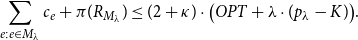 $$\sum_{e:e\in M_{\lambda}}c_e+\pi(R_{M_{\lambda}})\leq (2+\kappa) \cdot \big(OPT+\lambda\cdot(p_{\lambda}-K)\big).$$
Here, OPT represents the optimal value of the K-PCMTS for instance
 $\mathcal{I}$
;
$\mathcal{I}$
;
 $R_{M_{\lambda}}$
is the set of pairs still connected after removing
$R_{M_{\lambda}}$
is the set of pairs still connected after removing
 $M_{\lambda}$
; and
$M_{\lambda}$
; and
 $\kappa$
represents the total curvature of
$\kappa$
represents the total curvature of
 $\pi(\!\cdot\!)$
.
$\pi(\!\cdot\!)$
.
Proof. Let
 $M^*$
be an optimal solution; let
$M^*$
be an optimal solution; let
 $OPT=\sum_{e:e\in M^*}c_e+\pi(R_{M^*}) $
be the optimal value of the K-PCMTS on instance
$OPT=\sum_{e:e\in M^*}c_e+\pi(R_{M^*}) $
be the optimal value of the K-PCMTS on instance
 $\mathcal{I}$
. Then,
$\mathcal{I}$
. Then,
 $M^*$
is also a feasible solution for instance
$M^*$
is also a feasible solution for instance
 $\mathcal{I}_{\lambda}$
of the MTS for any
$\mathcal{I}_{\lambda}$
of the MTS for any
 $\lambda\geq 0$
, and
$\lambda\geq 0$
, and
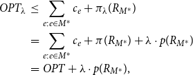 \begin{eqnarray} OPT_{\lambda}&\leq & \sum_{e:e\in M^*}c_e+\pi_{\lambda}(R_{M^*})\nonumber\\ &= &\sum_{e:e\in M^*}c_e+\pi(R_{M^*}) +\lambda\cdot p (R_{M^*})\nonumber\\ &=&OPT +\lambda\cdot p (R_{M^*}), \end{eqnarray}
where
 $OPT_{\lambda}$
is the optimal value on instance
$OPT_{\lambda}$
is the optimal value on instance
 $\mathcal{I}_{\lambda}$
of the MTS, and
$\mathcal{I}_{\lambda}$
of the MTS, and
 $R_{M^*}=\mathcal{P}\setminus D_{M^*}$
is the set of pairs still connected after removing
$R_{M^*}=\mathcal{P}\setminus D_{M^*}$
is the set of pairs still connected after removing
 $M^*$
.
$M^*$
.
Based on the definition of total curvature and
 $\pi_{\lambda}(\!\cdot\!)$
in (8), we have
$\pi_{\lambda}(\!\cdot\!)$
in (8), we have
 \begin{eqnarray} \kappa_{\lambda} &=&1-\min_{j:(s_j,t_j)\in \mathcal{P}}\frac{\pi_{\lambda}((s_j,t_j)|\mathcal{P}\setminus\{(s_j,t_j)\})}{\pi_{\lambda}(\{(s_j,t_j)\})}\nonumber\\ &=&1-\min_{j:(s_j,t_j)\in \mathcal{P}}\frac{\pi_{\lambda}(\mathcal{P})-\pi_{\lambda}(\mathcal{P}\setminus\{(s_j,t_j)\})}{\pi(\{(s_j,t_j)\})+\lambda\cdot p_j}\nonumber\\ &=&1-\min_{j:(s_j,t_j)\in \mathcal{P}}\frac{\pi(\mathcal{P})+\lambda\cdot p(\mathcal{P})-\pi(\mathcal{P}\setminus\{(s_j,t_j)\})-\lambda\cdot p(\mathcal{P}\setminus\{(s_j,t_j)\})}{\pi(\{(s_j,t_j)\})+\lambda\cdot p_j}\nonumber\\ &=&1-\min_{j:(s_j,t_j)\in \mathcal{P}}\frac{\pi((s_j,t_j)|\mathcal{P}\setminus\{(s_j,t_j)\})+\lambda\cdot p_j}{\pi(\{(s_j,t_j)\})+\lambda\cdot p_j}\nonumber\\ &\leq& 1-\min_{j:(s_j,t_j)\in \mathcal{P}}\frac{\pi((s_j,t_j)|\mathcal{P}\setminus\{(s_j,t_j)\})}{\pi(\{(s_j,t_j)\})}= \kappa. \end{eqnarray}
The objective value of
 $M_{\lambda}$
is
$M_{\lambda}$
is
 \begin{eqnarray*} &&\sum_{e:e\in M_{\lambda}}c_e+\pi(R_{M_{\lambda}})\\ &=&\sum_{e:e\in M_{\lambda}}c_e+\pi_{\lambda}(R_{M_{\lambda}})-\pi_{\lambda}(R_{M_{\lambda}})+\pi(R_{M_{\lambda}})\\ &\leq &(2+\kappa_{\lambda})\cdot OPT_{\lambda}-(1+\kappa_{\lambda})\cdot\sum_{j:(s_j,t_j)\in R_{M_{\lambda}}}\pi_{\lambda}(\{(s_j,t_j)\}|\mathcal{P}\setminus\{(s_j,t_j)\}) -\pi_{\lambda}(R_{M_{\lambda}})+\pi(R_{M_{\lambda}})\\ &= &(2+\kappa_{\lambda})\cdot OPT_{\lambda}-(1+\kappa_{\lambda})\cdot\sum_{j:(s_j,t_j)\in R_{M_{\lambda}}}\big(\pi_{\lambda}(\mathcal{P})-\pi_{\lambda}(\mathcal{P}\setminus\{(s_j,t_j)\})\big) -\lambda\cdot p(R_{M_{\lambda}})\\ &= &(2+\kappa_{\lambda})\cdot OPT_{\lambda}-(1+\kappa_{\lambda})\cdot\sum_{j:(s_j,t_j)\in R_{M_{\lambda}}}\big(\pi(\mathcal{P})-\pi(\mathcal{P}\setminus\{(s_j,t_j)\})+\lambda\cdot p_j\big) -\lambda\cdot p(R_{M_{\lambda}})\\ &\leq &(2+\kappa_{\lambda})\cdot OPT_{\lambda}-(2+\kappa_{\lambda})\cdot \lambda\cdot p(R_{M_{\lambda}})\\ &\leq &(2+\kappa_{\lambda})\cdot \big(OPT+ \lambda\cdot p(R_{M^*}) - \lambda\cdot p(R_{M_{\lambda}}) \big)\\ &= &(2+\kappa_{\lambda})\cdot \big(OPT+ \lambda\cdot (p({\mathcal{P}})-p( D_{M^*}))- \lambda\cdot(p({\mathcal{P}})-p_{\lambda}) \big)\\ &\leq &(2+\kappa)\cdot \big(OPT+ \lambda\cdot (p_{\lambda}-K) \big), \end{eqnarray*}
where the first inequality follows from Lemma 7, the second inequality follows from inequality (1), and the third inequality follows from inequality (12). The last inequality follows from inequalities (13) and
 $p( D_{M^*}) \geq K$
since
$p( D_{M^*}) \geq K$
since
 $M^*$
is a feasible solution to the K-PCMTS for instance
$M^*$
is a feasible solution to the K-PCMTS for instance
 $\mathcal{I}$
.
$\mathcal{I}$
.
Lemma 10. Algorithm 1 can be implemented in
 $O\big(\log \frac{ {p({\mathcal{P}})}\sum_{e:e\in E}c_e}{{\varepsilon c_{min}{\min_j p_j}}}\cdot (n^{6}\cdot \rho+n^{7})\big)$
, where
$O\big(\log \frac{ {p({\mathcal{P}})}\sum_{e:e\in E}c_e}{{\varepsilon c_{min}{\min_j p_j}}}\cdot (n^{6}\cdot \rho+n^{7})\big)$
, where
 $\rho$
is the running time of evaluating (the oracle for)
$\rho$
is the running time of evaluating (the oracle for)
 $\pi$
.
$\pi$
.
Proof. In each while loop, algorithm
 $\mathcal{A}$
is used once. We can find
$\mathcal{A}$
is used once. We can find
 $\lambda_1$
and
$\lambda_1$
and
 $\lambda_2$
satisfying
$\lambda_2$
satisfying
 $\lambda_1- \lambda_2 \leq \frac{\varepsilon c_{\min}}{p({\mathcal{P}})}$
after at most
$\lambda_1- \lambda_2 \leq \frac{\varepsilon c_{\min}}{p({\mathcal{P}})}$
after at most
 $O(\log \frac{\frac{1}{\min_j p_j} \sum_{e:e\in E}c_e+1}{\frac{\varepsilon c_{min}}{p({\mathcal{P}})}})=O(\log \frac{ {p({\mathcal{P}})}\sum_{e:e\in E}c_e}{{\varepsilon c_{min}{\min_j p_j}}})$
while loops. By Lemma 3, Algorithm 1 can be implemented in
$O(\log \frac{\frac{1}{\min_j p_j} \sum_{e:e\in E}c_e+1}{\frac{\varepsilon c_{min}}{p({\mathcal{P}})}})=O(\log \frac{ {p({\mathcal{P}})}\sum_{e:e\in E}c_e}{{\varepsilon c_{min}{\min_j p_j}}})$
while loops. By Lemma 3, Algorithm 1 can be implemented in
 $O\big(\log \frac{ {p({\mathcal{P}})}\sum_{e:e\in E}c_e}{{\varepsilon c_{min}{\min_j p_j}}}\cdot (n^{6}\cdot \rho+n^{7})\big)$
.
$O\big(\log \frac{ {p({\mathcal{P}})}\sum_{e:e\in E}c_e}{{\varepsilon c_{min}{\min_j p_j}}}\cdot (n^{6}\cdot \rho+n^{7})\big)$
.
Theorem. The objective value of M generated by Algorithm 1 is
 $$\sum_{e:e\in M}c_e+ \pi(R_M)\leq \big(\frac{8}{3}+\frac{4}{3}\cdot\kappa+9\cdot\varepsilon\big)\cdot OPT,$$
where
 $R_{M}=\mathcal{P}\setminus D_M$
is the set of pairs still connected after removing M, and
$R_{M}=\mathcal{P}\setminus D_M$
is the set of pairs still connected after removing M, and
 $\kappa$
is the total curvature of
$\kappa$
is the total curvature of
 $\pi(\!\cdot\!)$
.
$\pi(\!\cdot\!)$
.
Proof. If
 $p_0\geq K$
, then
$p_0\geq K$
, then
 $(M_{0},R_{0})$
is a feasible solution to K-PCMTS for instance
$(M_{0},R_{0})$
is a feasible solution to K-PCMTS for instance
 $\mathcal{I}$
, and its objective value is
$\mathcal{I}$
, and its objective value is
 \begin{eqnarray*}\sum_{e:e\in M_0}c_e+ \pi(R_{M_0})\leq (2+\kappa)\cdot \big(OPT+ 0\cdot (p_{0}-K) \big)= (2+\kappa)\cdot OPT , \end{eqnarray*}
where the inequality follows from Lemma 9. The theorem holds.
If
 $p_{\lambda_1} = K$
, then
$p_{\lambda_1} = K$
, then
 $(M_{\lambda_1},R_{\lambda_1})$
is a feasible solution to the K-PCMTS for instance
$(M_{\lambda_1},R_{\lambda_1})$
is a feasible solution to the K-PCMTS for instance
 $\mathcal{I}$
, and its objective value is
$\mathcal{I}$
, and its objective value is
 \begin{eqnarray*} \sum_{e:e\in M_{\lambda_1}}c_e+ \pi(R_{M_{\lambda_1}})\leq (2+\kappa)\cdot \big(OPT+ \lambda\cdot (p_{\lambda_1}-K) \big)=(2+\kappa)\cdot OPT, \end{eqnarray*}
where the inequality follows from Lemma 9. The theorem holds.
Then, we consider the case where
 $p_{\lambda_1}>K$
when the algorithm is terminated. Let
$p_{\lambda_1}>K$
when the algorithm is terminated. Let
 $\alpha=\frac{K-p_{\lambda_2}}{{p_{\lambda_1} -p_{\lambda_2}}}$
; Then, we have
$\alpha=\frac{K-p_{\lambda_2}}{{p_{\lambda_1} -p_{\lambda_2}}}$
; Then, we have
 $$\alpha\in (0,1), $$
by
 $p_{\lambda_1}>K$
and
$p_{\lambda_1}>K$
and
 $ p_{\lambda_2}<K$
such that
$ p_{\lambda_2}<K$
such that
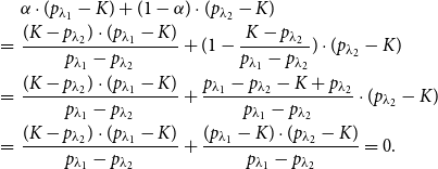 \begin{eqnarray} &&\alpha\cdot (p_{\lambda_1}-K)+(1-\alpha) \cdot (p_{\lambda_2}-K)\nonumber\\ &=& \frac{(K-p_{\lambda_2} )\cdot (p_{\lambda_1}-K)}{p_{\lambda_1}-p_{\lambda_2} }+ (1-\frac{K-p_{\lambda_2} }{p_{\lambda_1}-p_{\lambda_2} })\cdot (p_{\lambda_2}-K)\nonumber\\ &=& \frac{(K-p_{\lambda_2} )\cdot (p_{\lambda_1}-K)}{p_{\lambda_1}-p_{\lambda_2} }+ \frac{p_{\lambda_1}-p_{\lambda_2}-K+p_{\lambda_2} }{p_{\lambda_1}-p_{\lambda_2} }\cdot (p_{\lambda_2}-K)\nonumber\\ &=& \frac{(K-p_{\lambda_2} )\cdot (p_{\lambda_1}-K)}{p_{\lambda_1}-p_{\lambda_2} }+ \frac{(p_{\lambda_1}-K )\cdot (p_{\lambda_2}-K)}{p_{\lambda_1}-p_{\lambda_2} }=0\nonumber. \end{eqnarray}
Thus,
 \begin{eqnarray} && \alpha\cdot \big(\sum_{e:e\in M_{\lambda_1}}c_e+\pi(R_{M_{\lambda_1}})\big) +(1-\alpha)\cdot\big(\sum_{e:e\in M_{\lambda_2}}c_e+\pi(R_{M_{\lambda_2}})\big)\nonumber\\ &\leq &(2+\kappa)\cdot\alpha \cdot \big(OPT+ \lambda_1\cdot (p_{\lambda_1}-K) \big)+(2+\kappa)\cdot(1-\alpha)\cdot \big(OPT+ \lambda_2\cdot (p_{\lambda_2}-K) \big)\nonumber\\ &\leq &(2+\kappa)\cdot OPT+(2+\kappa)\cdot\alpha\cdot(\lambda_2+ \frac{\varepsilon c_{\min}}{p({\mathcal{P}})})\cdot(p_{\lambda_1}-K)+(2+\kappa)\cdot(1-\alpha)\cdot\lambda_2\cdot (p_{\lambda_2}-K)\nonumber\\ &=&(2+\kappa)\cdot OPT+(2+\kappa)\cdot\lambda_2\cdot\big(\alpha\cdot(p_{\lambda_1}-K)+ (1-\alpha) \cdot(p_{\lambda_2}-K) \big)\nonumber\\ &&+(2+\kappa)\cdot\alpha\cdot \frac{\varepsilon c_{\min}}{p({\mathcal{P}})}\cdot({p_{\lambda_1}-K})\nonumber\\ &=&(2+\kappa)\cdot OPT+(2+\kappa)\cdot\alpha\cdot \frac{\varepsilon c_{\min}}{p({\mathcal{P}})}\cdot({p_{\lambda_1}-K})\nonumber\\ &\leq & (2+\kappa)\cdot OPT+(2+\kappa)\cdot \varepsilon\cdot c_{\min}\nonumber\\ &\leq& (2+\kappa)\cdot (1+\varepsilon)\cdot OPT, \end{eqnarray}
where the first inequality follows from Lemma 9, the second inequality follows from
 $\lambda_1- \lambda_2 \leq \frac{\varepsilon c_{\min}}{p({\mathcal{P}})}$
, the third inequality follows from
$\lambda_1- \lambda_2 \leq \frac{\varepsilon c_{\min}}{p({\mathcal{P}})}$
, the third inequality follows from
 $\alpha\in (0,1)$
and
$\alpha\in (0,1)$
and
 $\frac{p_{\lambda_1}-K}{p({\mathcal{P}})}\leq 1$
by
$\frac{p_{\lambda_1}-K}{p({\mathcal{P}})}\leq 1$
by
 $p({\mathcal{P}}) \geq p_{\lambda_1}-K$
, and the last inequality follows from inequality (13).
$p({\mathcal{P}}) \geq p_{\lambda_1}-K$
, and the last inequality follows from inequality (13).
Case 1. If
 $\sum_{e:e\in M_{\lambda_2}}c_e+\pi(R_{M_{\lambda_2}})\leq \frac{2+\kappa}{3 \cdot\alpha }\cdot OPT$
, then the objective value of M is
$\sum_{e:e\in M_{\lambda_2}}c_e+\pi(R_{M_{\lambda_2}})\leq \frac{2+\kappa}{3 \cdot\alpha }\cdot OPT$
, then the objective value of M is
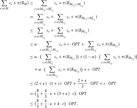 \begin{eqnarray*} \sum_{e:e\in M}c_e+\pi(R_{M}) &\leq & \sum_{e:e\in M_{\lambda_2}\cup M'_{\lambda_1} }c_e +\pi(R_{M_{\lambda_2}\cup M'_{\lambda_1}})\\ &=&\sum_{e:e\in M'_{\lambda_1}}c_e+\sum_{e:e\in M_{\lambda_2}}c_e+\pi(R_{M_{\lambda_2}\cup M'_{\lambda_1}})\\ &\leq &\sum_{e:e\in M'_{\lambda_1}}c_e+\sum_{e:e\in M_{\lambda_2}}c_e+\pi(R_{M_{\lambda_2}})\\ &\leq &\alpha\cdot\sum_{e:e\in M_{\lambda_1}\setminus M_{\lambda_2}}c_e+\varepsilon\cdot OPT+\sum_{e:e\in M_{\lambda_2}}c_e+\pi(R_{M_{\lambda_2}}) \\ &\leq &\alpha\cdot\big(\sum_{e:e\in M_{\lambda_1}}c_e+\pi(R_{M_{\lambda_1}})\big)+(1-\alpha) \cdot \big(\sum_{e:e\in M_{\lambda_2}}c_e+\pi(R_{M_{\lambda_2}})\big)\\ &&+\;\alpha \cdot \big(\sum_{e:e\in M_{\lambda_2}}c_e+\pi(R_{M_{\lambda_2}})\big)+\varepsilon\cdot OPT\\ &\leq &(2+\kappa)\cdot (1+\varepsilon)\cdot OPT+\frac{2+\kappa}{3}\cdot OPT+\varepsilon\cdot OPT\\ &=&\big(\frac{8}{3}+\frac{4}{3}\cdot\kappa+(3+\kappa)\cdot \varepsilon\big)\cdot OPT\\ &\leq&\big(\frac{8}{3}+\frac{4}{3}\cdot\kappa+4\cdot \varepsilon\big)\cdot OPT, \end{eqnarray*}
where the second inequality follows from
 $R_{M_{a}}\subseteq R_{M_{\lambda_2}}$
and the third inequality follows from Lemma 8: The fourth inequality follows from
$R_{M_{a}}\subseteq R_{M_{\lambda_2}}$
and the third inequality follows from Lemma 8: The fourth inequality follows from
 $\sum_{e:e\in M_{\lambda_1}\setminus M_{\lambda_2}}c_e\leq \sum_{e:e\in M_{\lambda_1}}c_e \leq\sum_{e:e\in M_{\lambda_1}}c_e+\pi(R_{M_{\lambda_1}})$
, the fifth inequality follows from inequality (14) and from the assumption that
$\sum_{e:e\in M_{\lambda_1}\setminus M_{\lambda_2}}c_e\leq \sum_{e:e\in M_{\lambda_1}}c_e \leq\sum_{e:e\in M_{\lambda_1}}c_e+\pi(R_{M_{\lambda_1}})$
, the fifth inequality follows from inequality (14) and from the assumption that
 $\sum_{e:e\in M_{\lambda_2}}c_e+\pi(R_{M_{\lambda_2}})\leq \frac{2+\kappa}{3 \cdot\alpha }\cdot OPT$
, and the last inequality follows from
$\sum_{e:e\in M_{\lambda_2}}c_e+\pi(R_{M_{\lambda_2}})\leq \frac{2+\kappa}{3 \cdot\alpha }\cdot OPT$
, and the last inequality follows from
 $\kappa\leq 1$
.
$\kappa\leq 1$
.
Case 2. If
 $\sum_{e:e\in M_{\lambda_2}}c_e+\pi(R_{M_{\lambda_2}})> \frac{2+\kappa}{3 \cdot\alpha}\cdot OPT$
, then the objective value of M is
$\sum_{e:e\in M_{\lambda_2}}c_e+\pi(R_{M_{\lambda_2}})> \frac{2+\kappa}{3 \cdot\alpha}\cdot OPT$
, then the objective value of M is
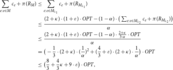 \begin{eqnarray*} \sum_{e:e\in M}c_e+\pi(R_{M}) &\leq & \sum_{e:e\in M_{\lambda_1}}c_e+\pi(R_{M_{\lambda_1}})\\ &\leq &\frac{(2+\kappa)\cdot (1+\varepsilon)\cdot OPT-(1-\alpha)\cdot \big(\sum_{e:e\in M_{\lambda_2}}c_e+\pi(R_{M_{\lambda_2}})\big)}{\alpha}\\ &\leq &\frac{(2+\kappa)\cdot (1+\varepsilon)\cdot OPT- (1-\alpha) \cdot \frac{2+\kappa}{3 \cdot\alpha}\cdot OPT}{\alpha}\\ &= &\big(-\frac{1}{3 }\cdot(2+\kappa)\cdot(\frac{1}{\alpha})^2+ (\frac{4}{3 }+ \varepsilon)\cdot(2+\kappa)\cdot \frac{1}{\alpha}\big)\cdot OPT \\ &\leq&\big(\frac{8}{3}+ \frac{4}{3}\kappa+9\cdot\varepsilon\big)\cdot OPT, \end{eqnarray*}
where the second inequality follows from inequality (14) and the third inequality follows from the assumption that
 $\sum_{e:e\in M_{\lambda_2}}c_e+\pi(R_{M_{\lambda_2}})> \frac{2+\kappa}{3 \cdot\alpha}\cdot OPT$
. The last inequality follows from
$\sum_{e:e\in M_{\lambda_2}}c_e+\pi(R_{M_{\lambda_2}})> \frac{2+\kappa}{3 \cdot\alpha}\cdot OPT$
. The last inequality follows from
 $\frac{1}{\alpha}\in (1,+\infty)$
,
$\frac{1}{\alpha}\in (1,+\infty)$
,
 $\kappa\in [0,1]$
and the following fact: The function
$\kappa\in [0,1]$
and the following fact: The function
 $f(x)= -\frac{1}{3}\cdot (2+\kappa)\cdot x^2 +(\frac{4}{3}+\varepsilon)\cdot (2+\kappa)\cdot x$
satisfies
$f(x)= -\frac{1}{3}\cdot (2+\kappa)\cdot x^2 +(\frac{4}{3}+\varepsilon)\cdot (2+\kappa)\cdot x$
satisfies
 $f(2+\frac{3}{2}\varepsilon) \geq f(x')$
for any
$f(2+\frac{3}{2}\varepsilon) \geq f(x')$
for any
 $x'\in [1,+\infty)$
, i.e.,
$x'\in [1,+\infty)$
, i.e.,
 $$f(\frac{1}{\alpha})\leq f(2+\frac{3}{2}\varepsilon)=(2+\kappa)(\frac{4}{3}+2\cdot\varepsilon+\frac{3}{4}\varepsilon^2) \leq \frac{8}{3}+ \frac{4}{3}\kappa+9\cdot\varepsilon ,~\forall \alpha\in(0,1).$$
Therefore, the theorem holds.
Corollary 11. Algorithm 1 is a tight
 $(\frac{8}{3}+\varepsilon)$
-approximation algorithm for the K-PCMTS with
$(\frac{8}{3}+\varepsilon)$
-approximation algorithm for the K-PCMTS with
 $\kappa=0$
; i.e., the penalty function is linear, which is a generalization of the k-prize-collecting multicut problem in trees. Thus, our algorithm improves upon the
$\kappa=0$
; i.e., the penalty function is linear, which is a generalization of the k-prize-collecting multicut problem in trees. Thus, our algorithm improves upon the
 $(4+\varepsilon)$
-approximation algorithm presented by Hou et al. (Reference Hou, Liu and Hou2020).
$(4+\varepsilon)$
-approximation algorithm presented by Hou et al. (Reference Hou, Liu and Hou2020).
Proof. Then, we use a simple example to illustrate that the approximation factor of Algorithm 1 is tight.
We are given an instance
 $\mathcal{I}=(V,E;\;\mathcal{P};\;K,\pi,c,p)$
of the K-PCMTS, which is shown in Figure 1, where
$\mathcal{I}=(V,E;\;\mathcal{P};\;K,\pi,c,p)$
of the K-PCMTS, which is shown in Figure 1, where
 $V=\{v_0,v_1,v_2,v_3,v_4,v_5\}$
,
$V=\{v_0,v_1,v_2,v_3,v_4,v_5\}$
,
 $E=\{e_1,e_2,e_3,e_4, e_5 \}$
, and
$E=\{e_1,e_2,e_3,e_4, e_5 \}$
, and
 $\mathcal{P}=\{(s_1,t_1),(s_2,t_2),(s_3,t_3),(s_4,t_4)\}$
, and the function
$\mathcal{P}=\{(s_1,t_1),(s_2,t_2),(s_3,t_3),(s_4,t_4)\}$
, and the function
 $\pi(\!\cdot\!)$
satisfies
$\pi(\!\cdot\!)$
satisfies
 $\pi(R)=0$
for any
$\pi(R)=0$
for any
 $R\subseteq \mathcal{P}$
; i.e.,
$R\subseteq \mathcal{P}$
; i.e.,
 $\pi(\!\cdot\!)$
is a linear function, and
$\pi(\!\cdot\!)$
is a linear function, and
 $\kappa=0$
. Pair
$\kappa=0$
. Pair
 $(s_1,t_1)$
is
$(s_1,t_1)$
is
 $(v_4,v_5)$
, both
$(v_4,v_5)$
, both
 $(s_2,t_2)$
and
$(s_2,t_2)$
and
 $(s_3,t_3)$
are
$(s_3,t_3)$
are
 $(v_2,v_3)$
, and
$(v_2,v_3)$
, and
 $(s_4,t_4)$
is
$(s_4,t_4)$
is
 $(v_0,v_1)$
. Given a positive number,
$(v_0,v_1)$
. Given a positive number,
 $\varepsilon^*>0$
, we define
$\varepsilon^*>0$
, we define
 \begin{eqnarray*} \left\{ \begin{split} &c_{e_1}= 1+3\varepsilon^*;\\ &c_{e_2}= \frac{4}{3};\\ &c_{e_3}= \frac{4}{3};\\ &c_{e_4}= \frac{2}{3}-\varepsilon^*;\\ &c_{e_5}= \frac{2}{3}-\varepsilon^*; \end{split}\right.~~~~~~~~~~~~~~~~~~~~~~ \left\{ \begin{split} &p_1=\frac{2}{3};\\ &p_2=\frac{1}{3}+\frac{1}{3}\varepsilon^*;\\ &p_3=\frac{1}{3}+\frac{1}{3}\varepsilon^*;\\ &p_4=1+\varepsilon^*;\\ &K=1+\frac{1}{2}\varepsilon^*. \end{split}\right. \end{eqnarray*}
It is easy to determine that the optimal multicut
 $M^*=\{e_1\}$
; its objective value is
$M^*=\{e_1\}$
; its objective value is
 $OPT=1+3\varepsilon^*$
.
$OPT=1+3\varepsilon^*$
.
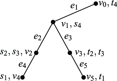
Figure 1. Instance
 $\mathcal{I}$
of the K-PCMTS.
$\mathcal{I}$
of the K-PCMTS.
For any
 $\lambda$
, we construct an instance
$\lambda$
, we construct an instance
 $\mathcal{I}_{\lambda}$
of the MTS as above, i.e., the penalty
$\mathcal{I}_{\lambda}$
of the MTS as above, i.e., the penalty
 $\pi_{\lambda}(j)=0+\lambda\cdot p_j$
for each
$\pi_{\lambda}(j)=0+\lambda\cdot p_j$
for each
 $(s_j,t_j)\in \mathcal{P}$
. For convenience, we define
$(s_j,t_j)\in \mathcal{P}$
. For convenience, we define
 $v_0$
as the root. When
$v_0$
as the root. When
 $\lambda=0$
,
$\lambda=0$
,
 $M_0=\emptyset$
, and all the pairs are connected. Thus,
$M_0=\emptyset$
, and all the pairs are connected. Thus,
 $M_0$
is not a feasible solution. Then, Algorithm 1 finds
$M_0$
is not a feasible solution. Then, Algorithm 1 finds
 $\lambda_1$
and
$\lambda_1$
and
 $\lambda_2$
satisfying
$\lambda_2$
satisfying
 $\lambda_1> \lambda_2$
,
$\lambda_1> \lambda_2$
,
 $\lambda_1- \lambda_2 \leq \frac{\varepsilon c_{min}}{p(\mathcal{P})}$
, and
$\lambda_1- \lambda_2 \leq \frac{\varepsilon c_{min}}{p(\mathcal{P})}$
, and
 $p_{\lambda_1}\geq K > p_{\lambda_2}$
by using a binary search over the interval
$p_{\lambda_1}\geq K > p_{\lambda_2}$
by using a binary search over the interval
 $[0, \frac{15+3\varepsilon^*}{1+\varepsilon^*}+1]$
.
$[0, \frac{15+3\varepsilon^*}{1+\varepsilon^*}+1]$
.
It is not difficult to prove that
 $M_\lambda$
is not a feasible solution if
$M_\lambda$
is not a feasible solution if
 $\lambda<1+\frac{2+3\varepsilon^*}{6+2\varepsilon^*}$
and that
$\lambda<1+\frac{2+3\varepsilon^*}{6+2\varepsilon^*}$
and that
 $M_\lambda$
is a feasible solution if
$M_\lambda$
is a feasible solution if
 $\lambda>1+\frac{2+3\varepsilon^*}{6+2\varepsilon^*}$
. Since
$\lambda>1+\frac{2+3\varepsilon^*}{6+2\varepsilon^*}$
. Since
 $\varepsilon^*$
is a given number, we can assume that Algorithm 1 obtains
$\varepsilon^*$
is a given number, we can assume that Algorithm 1 obtains
 $\lambda_1=1+\varepsilon^*$
and
$\lambda_1=1+\varepsilon^*$
and
 $\lambda_2=1$
. When
$\lambda_2=1$
. When
 $\lambda_1=1+\varepsilon^*$
, we have
$\lambda_1=1+\varepsilon^*$
, we have
 $\pi_{\lambda_1}(1)=\frac{2}{3}(1+\varepsilon^*)$
,
$\pi_{\lambda_1}(1)=\frac{2}{3}(1+\varepsilon^*)$
,
 $\pi_{\lambda_1}(2)=\pi_{\lambda_1}(3)=\frac{1}{3}(1+\varepsilon^*)^2\geq \frac{1}{3}+\frac{2}{3}\varepsilon^*$
, and
$\pi_{\lambda_1}(2)=\pi_{\lambda_1}(3)=\frac{1}{3}(1+\varepsilon^*)^2\geq \frac{1}{3}+\frac{2}{3}\varepsilon^*$
, and
 $\pi_{\lambda_1}(4)=(1+\varepsilon^*)^2<1+3\varepsilon^*$
, where the last inequality follows if
$\pi_{\lambda_1}(4)=(1+\varepsilon^*)^2<1+3\varepsilon^*$
, where the last inequality follows if
 $\varepsilon^*<1$
. By using
$\varepsilon^*<1$
. By using
 $\mathcal{A}$
, edges
$\mathcal{A}$
, edges
 $e_2$
and
$e_2$
and
 $e_3$
are selected, and
$e_3$
are selected, and
 $(s_4,t_4)$
is still connected. Thus,
$(s_4,t_4)$
is still connected. Thus,
 $M_{\lambda_1}=\{e_2,e_3\}$
is a feasible solution, and its objective is
$M_{\lambda_1}=\{e_2,e_3\}$
is a feasible solution, and its objective is
 $\frac{8}{3}$
. When
$\frac{8}{3}$
. When
 $\lambda_2=1$
, we have
$\lambda_2=1$
, we have
 $\pi_{\lambda_1}(1)=\frac{2}{3}$
,
$\pi_{\lambda_1}(1)=\frac{2}{3}$
,
 $\pi_{\lambda_1}(2)=\pi_{\lambda_1}(3)=\frac{1}{3}+\frac{1}{3}\varepsilon^*$
, and
$\pi_{\lambda_1}(2)=\pi_{\lambda_1}(3)=\frac{1}{3}+\frac{1}{3}\varepsilon^*$
, and
 $\pi_{\lambda_1}(4)=1+\varepsilon^*$
. By using
$\pi_{\lambda_1}(4)=1+\varepsilon^*$
. By using
 $\mathcal{A}$
, edges
$\mathcal{A}$
, edges
 $e_4$
and
$e_4$
and
 $e_5$
are selected, and
$e_5$
are selected, and
 $(s_2,t_2)$
,
$(s_2,t_2)$
,
 $(s_3,t_3)$
and
$(s_3,t_3)$
and
 $(s_4,t_4)$
are still connected. Thus,
$(s_4,t_4)$
are still connected. Thus,
 $M_{\lambda_2}$
is not a feasible solution because the disconnected profit is
$M_{\lambda_2}$
is not a feasible solution because the disconnected profit is
 $\frac{2}{3}<K$
. Thus, we need to construct a feasible solution by augmenting
$\frac{2}{3}<K$
. Thus, we need to construct a feasible solution by augmenting
 $M_{\lambda_2}$
with a carefully chosen subset,
$M_{\lambda_2}$
with a carefully chosen subset,
 $M'_{\lambda_1}\subseteq M_{\lambda_1}$
. In this process,
$M'_{\lambda_1}\subseteq M_{\lambda_1}$
. In this process,
 $(s_2,t_2)$
is assigned to
$(s_2,t_2)$
is assigned to
 $e_2$
, and
$e_2$
, and
 $(s_3,t_3)$
is assigned to
$(s_3,t_3)$
is assigned to
 $e_3$
. Since
$e_3$
. Since
 $p_1+p_2=p_1+p_3=1+\frac{1}{3}\varepsilon^*<K$
,
$p_1+p_2=p_1+p_3=1+\frac{1}{3}\varepsilon^*<K$
,
 $M'_{\lambda_1}=\{e_2,e_3\}$
. Thus,
$M'_{\lambda_1}=\{e_2,e_3\}$
. Thus,
 $M_{\lambda_2}\cup M'_{\lambda_1}=\{e_2,e_3,e_4,e_5\}$
, and its objective is
$M_{\lambda_2}\cup M'_{\lambda_1}=\{e_2,e_3,e_4,e_5\}$
, and its objective is
 $\frac{12}{3}-2\varepsilon^*$
.
$\frac{12}{3}-2\varepsilon^*$
.
Therefore,
 $M=M_{\lambda_1}=\{e_2,e_3\}$
and that
$M=M_{\lambda_1}=\{e_2,e_3\}$
and that
 \begin{eqnarray*} {\frac{\sum_{e:e\in M}c_e+\pi(R_{M})}{OPT}=\frac{\frac{8}{3}}{1+3\varepsilon^*}\rightarrow \frac{8}{3},{\rm when} ~\varepsilon^*\rightarrow 0.}\end{eqnarray*}
4. Numerical Experiments
The primary objective of this experimental study is to demonstrate the practical performance of Algorithm 1 and to compare it to that of a baseline method. Two datasets are utilized in the experiments. In the first experiment, we use a small-scale dataset, where the optimal solution and cost can be obtained. We evaluate the practical performance of our algorithm, and we compare it against those of the optimal solution and the GLH algorithm presented by Guo et al. (Reference Guo, Liu and Hou2023). In the second experiment, we use a large-scale dataset, where obtaining the optimal solution is not feasible. We evaluate the practical performance of our algorithm and compare it against that of the GLH algorithm.
Implementation details. The machine used for the experiments is equipped with an Intel(R) Core(TM) i9-10850H (3.60 GHz) CPU and 64 GB of main memory. The OS is Windows 11.
Datasets. Each dataset utilized in the study consists of 100 instances of the K-PCMTS. All instances within a dataset share the same level l of the tree and the same number m of pairs. The tree structure of each dataset is a complete binary tree with l levels. The weights associated with each edge in the tree are randomly generated, adhering to predefined ranges. From this complete binary tree, m pairs are randomly selected. For each pair, profit and penalty values are generated, following an average distribution within predefined ranges.
Submodular penalty function. We use the following nondecreasing submodular function for the experiments:
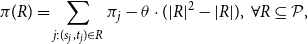 $$\pi(R)=\sum_{j:(s_j,t_j)\in R}\pi_j-\theta\cdot (|R|^2-|R|),~\forall R\subseteq \mathcal{P},$$
where
 $\theta$
is a positive number.
$\theta$
is a positive number.
Experimental procedures. To obtain the optimal value for the K-PCMTS, we utilize the open-source IBM tool Cplex to solve the integer program (5). For comparison purposes, we also execute the GLH algorithm of the K-prize-collecting set cover problem proposed by Guo et al. (Reference Guo, Liu and Hou2023). Let the source–sink pair set be the ground set; let each edge be a set whose elements are the disconnected pairs after removing this edge. For each pair
 $(s_j,t_j)$
, let its penalty be
$(s_j,t_j)$
, let its penalty be
 $\pi(\{(s_j,t_j)\})$
. The GLH algorithm can find a feasible solution for the K-PCMTS. In the first experiment, we compare the objective values obtained by Algorithm 1 against both the optimal value and the objective value obtained by the GLH algorithm. This evaluation is conducted on a small-scale dataset, considering various parameter settings for
$\pi(\{(s_j,t_j)\})$
. The GLH algorithm can find a feasible solution for the K-PCMTS. In the first experiment, we compare the objective values obtained by Algorithm 1 against both the optimal value and the objective value obtained by the GLH algorithm. This evaluation is conducted on a small-scale dataset, considering various parameter settings for
 $\theta$
. In the second experiment, we compare Algorithm 1 solely with the GLH algorithm, utilizing a large-scale dataset. The experiments involve varying the values of parameters l and m to assess the performance of the algorithm in various scenarios.
$\theta$
. In the second experiment, we compare Algorithm 1 solely with the GLH algorithm, utilizing a large-scale dataset. The experiments involve varying the values of parameters l and m to assess the performance of the algorithm in various scenarios.
Numerical results. Figure 2 illustrates the objective values obtained by Algorithm 1, the optimal value, and the GLH algorithm for various
 $\theta$
values on a small-scale dataset with
$\theta$
values on a small-scale dataset with
 $l=5$
and
$l=5$
and
 $m=5$
. Furthermore, Figure 3 displays the objective values of Algorithm 1 and the GLH algorithm for varying m values on a large-scale dataset with
$m=5$
. Furthermore, Figure 3 displays the objective values of Algorithm 1 and the GLH algorithm for varying m values on a large-scale dataset with
 $\theta=0.2$
and
$\theta=0.2$
and
 $l=40$
.Figure 3 has not been mentioned in the text. Please cite the figure in the relevant place in the text. The results highlight several key findings. First, the results validate that the practical performance of Algorithm 1 is much better than is the theoretical performance, which the objective value of Algorithm 1 is less than 130% compared with the optimal value in most cases. Moreover, it is evident that the gap between the objective values generated by Algorithm 1 and by the GLH algorithm widens with increasing values of
$l=40$
.Figure 3 has not been mentioned in the text. Please cite the figure in the relevant place in the text. The results highlight several key findings. First, the results validate that the practical performance of Algorithm 1 is much better than is the theoretical performance, which the objective value of Algorithm 1 is less than 130% compared with the optimal value in most cases. Moreover, it is evident that the gap between the objective values generated by Algorithm 1 and by the GLH algorithm widens with increasing values of
 $\theta$
and m, which agrees with our expectations.
$\theta$
and m, which agrees with our expectations.
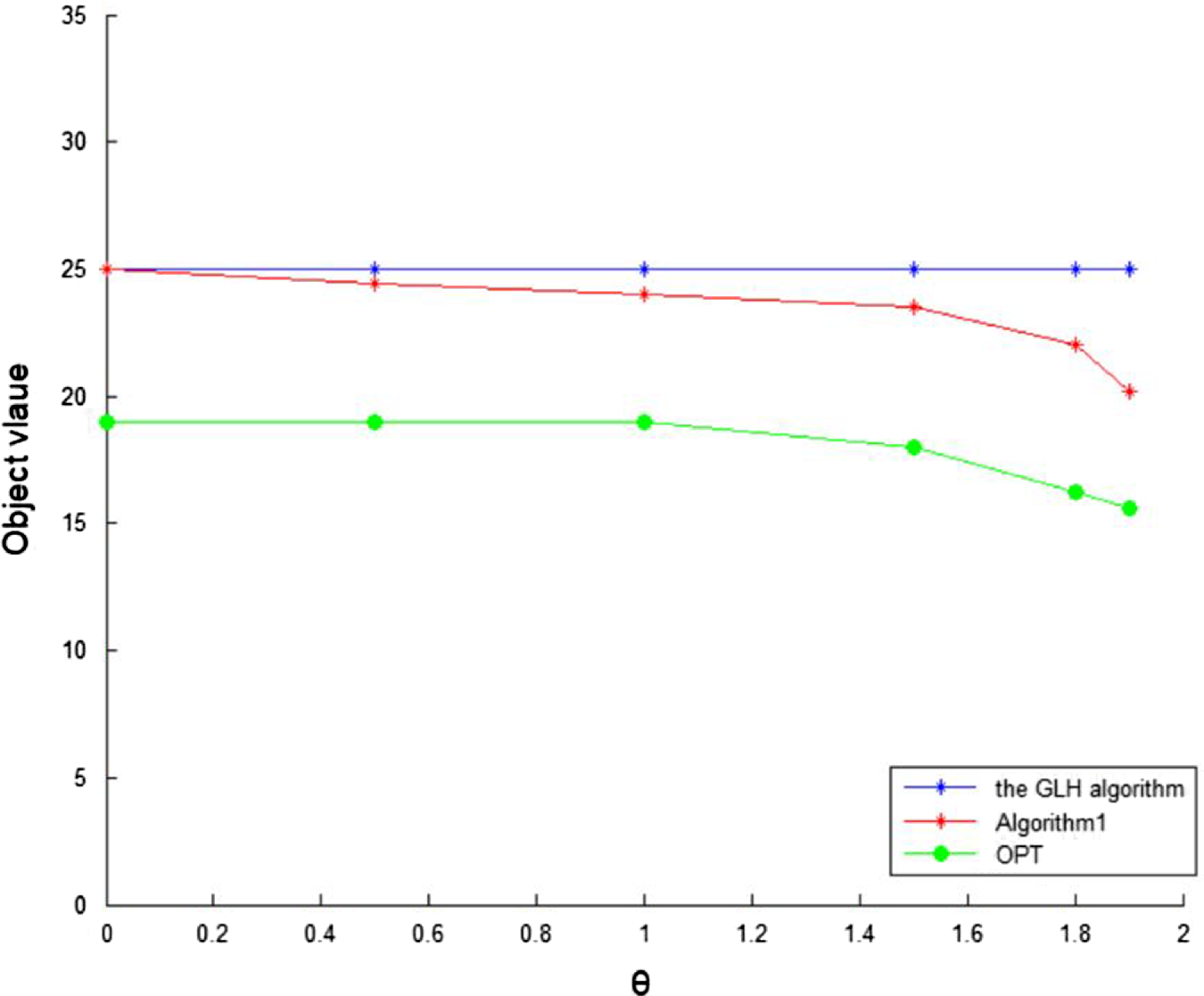
Figure 2. Solution quality for a small-scale dataset.
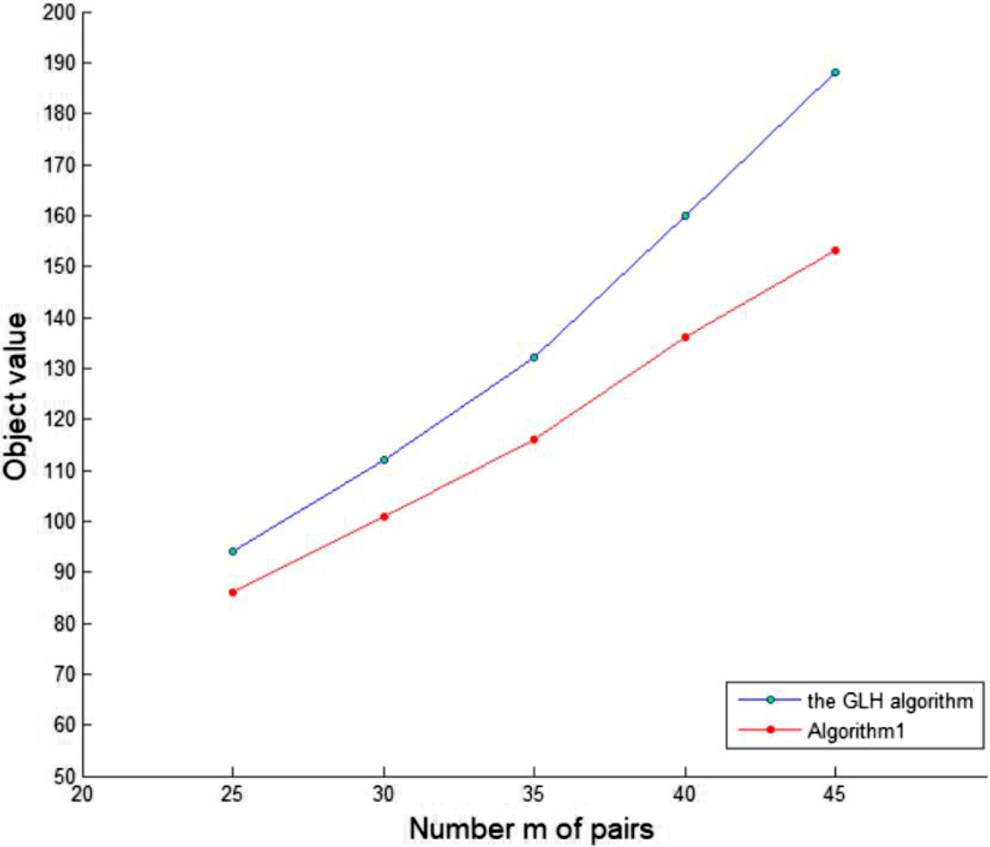
Figure 3. Performances of Algorithm 1 against the linear algorithm.
5. Final Remarks
We consider the K-prize-collecting multicut problem in trees with submodular penalties. This problem is a generalization of the minimum multicut problem in trees, the partial multicut problem in trees, the generalized partial multicut problem in trees, the prize-collecting multicut problem in trees, the multicut problem in trees with submodular penalties, and the k-prize-collecting multicut problem in trees. These problems have been widely studied. In this paper, we present a combinatorial polynomial-time
 $(\frac{8}{3}+\frac{4}{3}\kappa+ \varepsilon)$
-approximation algorithm, where
$(\frac{8}{3}+\frac{4}{3}\kappa+ \varepsilon)$
-approximation algorithm, where
 $\varepsilon$
is any fixed positive number and
$\varepsilon$
is any fixed positive number and
 $\kappa$
is the total curvature of the submodular function.
$\kappa$
is the total curvature of the submodular function.
Garg et al. (Reference Garg, Vazirani and Yannakakis1997) presented a lower bound showing that there is no algorithm with an approximation factor less than 2 for the multicut problem in trees. The K-prize-collecting multicut problem in trees with submodular penalties generalizes the multicut problem in trees, and the lower bound is at least 2. There is a large gap between our algorithm and this lower bound.
In many realistic applications, many functions are difficult to compute; we usually have only a noisy oracle (such as multiplicative or additive noise) that returns an approximate value of the function (Yang et al. Reference Yang, Xu, Cheng, Gao and Du2019). It is obvious that the submodular function under noise is a set function and that there is no polynomial algorithm for the set function minimization problem, which means that our algorithm cannot solve the problem under noise. It is thus of interest to design a constant approximation algorithm for this problem under noise.
Acknowledgements.
The work was partly supported by the National Natural Science Foundation of China (No. 12071417), the Yunnan Provincial Research Foundation for Basic Research, China (Nos. 202401AT070442, 202301AU070197), and the Project of Yunnan Provincial Department of Education Science Research Fund (No. 2023J0014).


