


1. Introduction
Swirling fluid flows are ubiquitous both in nature and in technological applications. They are found everywhere: from gigantic vortices existing on galactic, star and planetary scales to vortices created by microswimmers. Encountering them is an everyday reality and it is probably safe to say that any movement through a fluid or any flow of a fluid around a solid object can potentially create a vortex. The appearance of vortices is closely linked to the instability of the predecessor states that vary widely in their configurations and physical features while the resulting fluid vortices appear very similar regardless of how and where they have been generated. This may create an impression that vortices generated in geometrically similar domains in flows with similar kinematic characteristics are caused by the same physical mechanisms. However, this may be far from reality and each situation resulting in the vortex formation requires an individual consideration and analysis.
The study that we undertake here is the prime example of this. Electromagnetically driven circumferential flow in a shallow annular channel that we described in detail in Part 1 develops an experimentally observable robust system of propagating free-surface vortices (Pérez-Barrera et al. Reference Pérez-Barrera, Pérez-Espinoza, Ortiz, Ramos and Cuevas2015; Pérez-Barrera, Ortiz & Cuevas Reference Pérez-Barrera, Ortiz and Cuevas2016; Pérez-Barrera et al. Reference Pérez-Barrera, Ramírez-Zúñiga, Grespan, Cuevas and del Río2019) that superficially look very similar to those observed in other circular flows. Despite this fact, their methodic analysis that we report in the current paper shows that there are significant differences between their natures. Before we focus on such an analysis, here we present a brief overview of other rotational flows that may be tempting to consider as at least partial analogues of flows studied here.
The azimuthal flow induced in an annular channel by the action of the bulk Lorentz force is confined between a stationary solid bottom and a free surface and, thus, is characterised by a non-trivial dependence of the fluid velocity components on the vertical coordinate. In an alternative setting the variation of flow characteristics in the axial direction can be enforced by a differential rotation of the top and bottom solid walls (horizontal disks) enclosing a cylindrical vessel. Experimental observations (e.g. Lopez et al. Reference Lopez, Hart, Marques, Kittelman and Shen2002; Moisy et al. Reference Moisy, Doaré, Pasutto, Daube and Rabaud2004) show that rotationally symmetric flow between differentially spinning end walls becomes unstable with respect to rotating waves with spiral, polygonal or star-shaped planforms. They occupy a large portion of a horizontal cross-section of a cylinder originating near its axis and extending toward the outer stationary side wall. The geometry of such waves differs drastically from a strongly localised vortex system observed in electromagnetically driven flows that we consider here.
When closely spaced top and bottom end walls co-rotate inside a stationary cylinder (shrouded configuration typical of computer hard-disk drives pre-dating solid state memory elements), the instability patterns take the form of vortices moving circumferentially closer to the outer wall, where the rotationally symmetric background flow develops a pair of toroidal counter-circulating rolls outside the inner solid-body-rotation core (Abrahamson, Eaton & Koga Reference Abrahamson, Eaton and Koga1989). At higher wall rotation speeds, when such vortices become sufficiently strong, they deform the inner-core flow existing near the axis of the cylinder so that its horizontal cross-section assumes a polygonal form (Herrero, Giralt & Humpfrey Reference Herrero, Giralt and Humpfrey1999). This indicates that the so-created vortices are essentially columnar and that they penetrate deeply into the bulk of fluid away from the rotating end walls (Randriamampianina, Schiestel & Wilson Reference Randriamampianina, Schiestel and Wilson2001; Poncet & Chauve Reference Poncet and Chauve2007). Unlike symmetric viscous forcing occurring in boundary layers developing on the rotating top and bottom end walls, electromagnetic Lorentz bulk forcing considered here varies both vertically and radially. It does not produce a solid-body-rotation core and the resulting free-surface vortices remain relatively shallow and do not penetrate into the bulk of fluid sufficiently deeply to exert their influence on the background flow there.
When the top and bottom end walls of an experimental set-up consist of differentially co-rotating concentric disk and ring sections, a cylindrical layer is formed at their border referred to as a Stewartson layer (Stewartson Reference Stewartson1957). Its stability was investigated in, for example, Früh & Read (Reference Früh and Read1999), Schaeffer & Cardin (Reference Schaeffer and Cardin2005) and von Larcher et al. (Reference von Larcher, Viazzo, Harlander, Vincze and Randriamampianina2018) showing that a number of vortices arise at the outer edge of such a layer resembling free-surface vortices we aim to study here. Even more similarly looking (when viewed from above) instability patterns to those discussed here occur in systems where the top and bottom end walls consist of counter-rotating concentric disk and ring sections (e.g. Rabaud & Couder Reference Rabaud and Couder1983; Chomaz et al. Reference Chomaz, Rabaud, Basdevnt and Couder1988; Bergeron et al. Reference Bergeron, Coutsias, Lynov and Nielsen2000). Such a set-up ensures the creation of a cylindrical shear layer at the ring/disk border that subsequently experiences classical Kelvin–Helmholtz instability with very regularly spaced ‘cat eye’ vortices. Again such vortices are essentially columnar and their radial position is fixed by the location of the border of the counter-rotating sections of the end walls while in flows considered here the location of vortices varies depending on the values of the Reynolds number and the meridional aspect ratio of the fluid layer.
One of the important practical applications of rotating flows discussed above is the laboratory modelling of large-scale atmospheric vortices and circulations (e.g. Niino & Misawa Reference Niino and Misawa1984; Früh & Read Reference Früh and Read1999). However, while these natural phenomena do involve rotating fluid, they differ fundamentally from the laboratory experiments mentioned above because the forcing causing atmospheric vortices does not come from the boundaries but is rather generated in the bulk of fluid/air (e.g. Coriolis force). To reduce this disparity between nature and laboratory experiments, the use of electromagnetic bulk forcing was suggested replacing non-conducting fluids with electrolytes carrying an electric current and interacting with the externally applied magnetic field (Dolzhanskii, Krymov & Manin Reference Dolzhanskii, Krymov and Manin1990; Bondarenko, Gak & Gak Reference Bondarenko, Gak and Gak2002; Kenjeres Reference Kenjeres2011, and references therein). In such experiments the flow within an annular channel bounded by stationary walls was created by means of the bulk Lorentz force arising due to the interaction of the radial electric current and the externally applied vertical magnetic field. In this set-up, the shear layer, the instability of which leads to the formation of the observed vortices, was created by changing the direction of the magnetic field to opposite at some radial location within the channel (a set of adjacent co-axial ring magnets with opposite vertical polarisations was used to achieve this in experiments). As a result, the induced Lorentz force drives the fluid clockwise or anticlockwise on different sides of the field-inversion line. A well-defined system of Kelvin–Helmholtz vortices develops at the boundary between the two circular regions with anti-parallel Lorentz forcing (Dovzhenko, Novikov & Obukhov Reference Dovzhenko, Novikov and Obukhov1979; Dovzhenko, Obukhov & Ponomarev Reference Dovzhenko, Obukhov and Ponomarev1981). Such vortices are almost equivalent to those observed in experiments with counter-rotating ring–disk set-ups described above even though the solid-body-rotation core flow does not exist in the background flow in this case.
The main feature that makes the set-up considered in this study unique and different from all other flow settings described above is that here the magnetic field is created by a single vertically polarised permanent magnet. This means that the vertical component of the applied magnetic field does not change its direction and the Lorentz force drives the fluid azimuthally in the same sense everywhere in the flow domain with no internal shear layer created. Yet, a prominent vortex system still develops, which, clearly, is not directly associated with the flow shear. The simplicity of such a set-up makes the discovered vortex generation mechanism attractive for applications in microstirrer technology (Piedra et al. Reference Piedra, Flores, Ramírez, Figueroa, Piñeirua and Cuevas2023), which motivated the original experimental studies of Pérez-Barrera et al. (Reference Pérez-Barrera, Ortiz and Cuevas2016). In this regard, it is also worthwhile mentioning that electromagnetically forced flows are much easier to generate, maintain and control than their mechanically driven counterparts because the strength and the direction of the Lorentz force are easily varied by changing the magnitude and direction of an electric current flowing between the electrodes. Interesting experiments on generating isolated vortices by a current pulse in a rotating electrolyte have been described, for example, in Cruz Gómez, Zavala Sansón & Pinilla (Reference Cruz Gómez, Zavala Sansón and Pinilla2013). More recent experiments with electromagnetically driven flows in cylindrical and spherical configurations with various magnetic field orientations and electrode placements reported in Acosta-Zamora & Beltrán (Reference Acosta-Zamora and Beltrán2022), Frick et al. (Reference Frick, Mandrykin, Eltischev and Kolesnichenko2022) and Proal et al. (Reference Proal, Domíguez-Lozoya, Figueroa, Rivero and Piedra2023) further demonstrate remarkable versatility of this method for inducing easily controllable vortical flows.
Having pointed out important physical differences distinguishing the currently studied set-up from rotational flows considered in the literature previously in this paper we also make a rather important observation: while details of primary axisymmetric flows and their physical excitation mechanisms may differ drastically, the development of their instabilities leading to secondary and tertiary flow patterns frequently follows similar scenarios. In particular, electromagnetically induced flow considered here experiences pure hydrodynamic instabilities that have a qualitative structure closely resembling that found in mechanically driven systems. Such similarities will be highlighted in the main body of the paper.
Our previous studies showed that, depending on the governing parameters, flow patterns arising in a thin annular electrolyte layer open from the top and driven circumferentially by the Lorentz force consist of the base azimuthally invariant steady fluid motion that may become unstable giving rise to a robust vortex system appearing on the free surface. In Suslov, Pérez-Barrera & Cuevas (Reference Suslov, Pérez-Barrera and Cuevas2017) two types of background flow were identified and McCloughan & Suslov (Reference McCloughan and Suslov2020a) showed that one of them, type 1, remains linearly stable, while the other (type 2 containing the secondary circulation region) is unstable with respect to propagating free-surface vortices. Both of these studies also demonstrated that the type 1 and 2 steady states cease to exist when Lorentz forcing exceeds a certain value while vortices are still observed in experiments (Pérez-Barrera et al. Reference Pérez-Barrera, Ortiz and Cuevas2016). Therefore, a weakly nonlinear study was undertaken in Part 1 (McCloughan & Suslov Reference McCloughan and Suslov2024) that indicated the presence of yet another, type 3, steady azimuthally invariant flow state for large forcing. In Part 2 we investigate the detailed stability characteristics of this newly discovered state. We confirm that it is responsible for the long-term existence of free-surfaces vortices while unstable type 2 flows may only influence the vortex formation transiently. We also identify qualitative bifurcation features of the perturbed type 3 flow that are similar to those reported for other physically different flow set-ups, thus confirming their universal nature.
The structure of the paper is as follows. In § 2 we formulate the mathematical model and describe the computational approach used to obtain various numerical results discussed in detail in § 3. They confirm the existence of the type 3 steady azimuthally invariant background flow, predicted by the asymptotic analysis presented in Part 1 over a wide range of the governing parameters, shed light on the temporal evolution of the flow leading to such a steady solution and determine characteristics of the instability modes resulting in experimentally observable vortices. The variation of instability patterns with the strength of forcing characterised by the Reynolds number and with the meridional aspect ratio of the channel are also discussed in this section. In § 4 we demonstrate the robustness and relevance of the obtained numerical results to realistic experiments despite several idealisations we introduced to make analytical and numerical progress. Concluding remarks outlining directions for subsequent investigation are given in § 5.
2. Problem formulation and details of the numerical procedure
2.1. Governing equations
As in Part 1 (McCloughan & Suslov Reference McCloughan and Suslov2024), we consider a layer of an electrolyte filling an annular channel with the inner and outer radii  $R_1$ and
  $R_2$, respectively. The top surface of the layer is free and the cylindrical side walls are formed by copper electrodes between which the total radial electric current
 \begin{equation} I_0\approx\frac{2{\rm \pi}\sigma_eh\Delta\phi_0}{\ln(R_2/R_1)}\end{equation}
flows, where  $\sigma _e$ is the electric conductivity of an electrolyte,
  $\Delta \phi _0$ is the applied electric potential difference between the electrodes and
  $h$ is the electrolyte depth. The system is placed in the axisymmetric magnetic field
  $\boldsymbol {B}=[B_r(r,z),0,B_z(r,z)]$ (
 $r$,
$r$,  $\theta$ and
  $z$ are the radial, azimuthal and vertical coordinates, respectively), created by a vertically polarised disk magnet as described in Suslov et al. (Reference Suslov, Pérez-Barrera and Cuevas2017). It is characterised by the magnitude
  $B_0$ at the lower inner corner of the meridional channel cross-section
  $\theta =$const. The distribution of the scaled vertical component
  $B_z$ of the magnetic field above the surface of the magnet is illustrated in figure 1. The interaction of the electric current and the magnetic field causes a predominantly azimuthal Lorentz force that drives the electrolyte flow without an external mechanical intervention.

Figure 1. The distribution of the vertical component  $B_z$ of the magnetic field above a disk magnet. The field is scaled so that its magnitude in the left bottom corner of the plot is unity. The influence of the magnetic field decay with the vertical distance
  $z^*$ from the magnet on the flow topology was detailed previously in Suslov et al. (Reference Suslov, Pérez-Barrera and Cuevas2017).
The non-dimensional governing equations describing azimuthally invariant flow and the corresponding boundary conditions can be written in a matrix operator form as
 \begin{equation} {\mathcal{B}}\partial_t\boldsymbol{w}={\mathcal{L}}\boldsymbol{w}+{\mathcal{N}}(\boldsymbol{w})+{\mathcal{H}}, \end{equation}
where the vector of unknown flow quantities
 \begin{equation} \boldsymbol{w}=[{\tilde{\phi}},u,v,w,p]^{\rm T}\end{equation}
includes the flow-induced variation  ${\tilde {\phi }}$ of the total electric potential
 \begin{equation} \phi=\dfrac{\ln\dfrac{r}{\alpha-1}}{\ln\dfrac{\alpha+1}{\alpha-1}} +\epsilon^2{{\textit{Ha}}}^2{\tilde{\phi}}(r,z), \end{equation}
the velocity components in the radial, azimuthal and vertical directions, and the pressure, respectively. The operator  ${\mathcal {B}}$ is the block-diagonal matrix with
  ${\mathcal {B}}_{ii}={\mathcal {I}}$,
  $i=2,3,4$, where
  ${\mathcal {I}}$ is the identity matrix with zero rows corresponding to the boundary points
  $r=\alpha \pm 1$ and
  $z=\pm 1$ and the rest of the blocks being zero. The
  $5\times 5$ block operator
  ${\mathcal {L}}$ corresponding to the bulk of fluid is defined as
 \begin{equation} \left. \begin{gathered}
{\mathcal{L}}_{11}=\partial_{zz}
+\epsilon^2\left(\partial_{rr}+\dfrac{\partial_r}{r}\right),\quad
{\mathcal{L}}_{13}=B_r\partial_z-B_z\left(\partial_r+\dfrac{1}{r}\right),\\
{\mathcal{L}}_{22}=-\dfrac{{{\textit{Ha}}}^2}{\epsilon^2{\textit{Re}}}B_z^2
+\dfrac{1}{{\textit{Re}}}\left(\partial_{rr}+\dfrac{\partial_r}{r}-\dfrac{1}{r^2}
+\dfrac{1}{\epsilon^2}\partial_{zz}\right),\quad{\mathcal{L}}_{24}=\frac{{{\textit{Ha}}}^2}{{\textit{Re}}}B_rB_z,\\
{\mathcal{L}}_{25}=-\partial_r,\quad
{\mathcal{L}}_{31}=\frac{{{\textit{Ha}}}^2}{{\textit{Re}}}(B_z\partial_r-B_r\partial_z),\\
{\mathcal{L}}_{33}=\dfrac{1}{{\textit{Re}}}\left(\partial_{rr}+\dfrac{\partial_r}{r}-\dfrac{1}{r^2}+\dfrac{\partial_{zz}}{\epsilon^2}\right)
-\dfrac{{{\textit{Ha}}}^2}{{\textit{Re}}}\left(B_r^2+\dfrac{B_z^2}{\epsilon^2}\right),\\
{\mathcal{L}}_{42}=\dfrac{{{\textit{Ha}}}^2}{\epsilon^2{\textit{Re}}}B_zB_r,\quad
{\mathcal{L}}_{44}=-\dfrac{{{\textit{Ha}}}^2}{{\textit{Re}}}B_r^2
+\dfrac{1}{{\textit{Re}}}\left(\partial_{rr}+\dfrac{\partial_r}{r}
+\dfrac{\partial_{zz}}{\epsilon^2}\right),\\
{\mathcal{L}}_{45}=-\dfrac{\partial_z}{\epsilon^2},\quad
{\mathcal{L}}_{52}=\partial_r+\dfrac{1}{r},\quad{\mathcal{L}}_{54}=\partial_z.
\end{gathered} \right\}
\end{equation}
\begin{equation} \left. \begin{gathered}
{\mathcal{L}}_{11}=\partial_{zz}
+\epsilon^2\left(\partial_{rr}+\dfrac{\partial_r}{r}\right),\quad
{\mathcal{L}}_{13}=B_r\partial_z-B_z\left(\partial_r+\dfrac{1}{r}\right),\\
{\mathcal{L}}_{22}=-\dfrac{{{\textit{Ha}}}^2}{\epsilon^2{\textit{Re}}}B_z^2
+\dfrac{1}{{\textit{Re}}}\left(\partial_{rr}+\dfrac{\partial_r}{r}-\dfrac{1}{r^2}
+\dfrac{1}{\epsilon^2}\partial_{zz}\right),\quad{\mathcal{L}}_{24}=\frac{{{\textit{Ha}}}^2}{{\textit{Re}}}B_rB_z,\\
{\mathcal{L}}_{25}=-\partial_r,\quad
{\mathcal{L}}_{31}=\frac{{{\textit{Ha}}}^2}{{\textit{Re}}}(B_z\partial_r-B_r\partial_z),\\
{\mathcal{L}}_{33}=\dfrac{1}{{\textit{Re}}}\left(\partial_{rr}+\dfrac{\partial_r}{r}-\dfrac{1}{r^2}+\dfrac{\partial_{zz}}{\epsilon^2}\right)
-\dfrac{{{\textit{Ha}}}^2}{{\textit{Re}}}\left(B_r^2+\dfrac{B_z^2}{\epsilon^2}\right),\\
{\mathcal{L}}_{42}=\dfrac{{{\textit{Ha}}}^2}{\epsilon^2{\textit{Re}}}B_zB_r,\quad
{\mathcal{L}}_{44}=-\dfrac{{{\textit{Ha}}}^2}{{\textit{Re}}}B_r^2
+\dfrac{1}{{\textit{Re}}}\left(\partial_{rr}+\dfrac{\partial_r}{r}
+\dfrac{\partial_{zz}}{\epsilon^2}\right),\\
{\mathcal{L}}_{45}=-\dfrac{\partial_z}{\epsilon^2},\quad
{\mathcal{L}}_{52}=\partial_r+\dfrac{1}{r},\quad{\mathcal{L}}_{54}=\partial_z.
\end{gathered} \right\}
\end{equation}
The remaining blocks in  ${\mathcal {L}}$ are zero. The vector of nonlinearities
  ${\mathcal {N}}(\boldsymbol {w})$ is
 \begin{equation}
{\mathcal{N}}(\boldsymbol{w})=\left[0,\,\frac{v^2}{r}-u\partial_ru-w\partial_z
u,
-u\partial_rv-\frac{uv}{r}-w\partial_zv,\,-u\partial_rw-w\partial_zw,\,0\right]^{\rm
T}.
\end{equation}
\begin{equation}
{\mathcal{N}}(\boldsymbol{w})=\left[0,\,\frac{v^2}{r}-u\partial_ru-w\partial_z
u,
-u\partial_rv-\frac{uv}{r}-w\partial_zv,\,-u\partial_rw-w\partial_zw,\,0\right]^{\rm
T}.
\end{equation}
The constant forcing vector  ${\mathcal {H}}$ is
 \begin{equation} {\mathcal{H}}=\left[0,0,\frac{B_z}{r\epsilon^2{\textit{Re}}\ln((\alpha+1)/(\alpha-1))}, 0,0\right]^{\rm T}.\end{equation}
 The above non-dimensional form of the equations contains three governing parameters: the meridional aspect ratio of the layer  $\epsilon$ and Hartmann and Reynolds numbers
  ${{{Ha}}}$ and
  ${{Re}}$, respectively defined as
 \begin{equation} \epsilon=\frac{h}{R_2-R_1},\quad {{\textit{Ha}}}^2=\frac{\sigma_eB_0^2h^2}{4\mu},\quad {\textit{Re}}=\frac{\rho U_0(R_2-R_1)}{2\mu}, \end{equation}
where the velocity scale is  $U_0=({\sigma _e\Delta \phi _0B_0h^2})/({2\mu (R_2-R_1)})$. Here
  $\mu$ and
  $\rho$ are the dynamic viscosity and the density of the electrolyte, respectively.
The no-slip/no-penetration velocity boundary conditions at the cylindrical electrodes and non-conducting bottom are
 \begin{equation} u=v=w=0\quad\text{at }z=-1\text{ and at }r=\alpha\pm1,\end{equation}
where  $\alpha =({R_2+R_1})/({R_2-R_1})$ (
 $\alpha =1.84$ is chosen to match the experimental set-up of Pérez-Barrera et al. Reference Pérez-Barrera, Pérez-Espinoza, Ortiz, Ramos and Cuevas2015, Reference Pérez-Barrera, Ortiz and Cuevas2016). The tangential stress-free condition at the stationary flat free surface is
 \begin{equation} w=\partial_zu=\partial_zv=0\quad \text{at }z=1.\end{equation}
The boundary conditions for the electric potential at the electrode surfaces, the non-conducting bottom and the free surface are
 \begin{gather} {\tilde{\phi}}=0\quad\text{at }r=\alpha\pm1,\end{gather}
 \begin{gather} \partial_z{\tilde{\phi}}=0\quad \text{at }z=-1\quad\text{and}\quad \partial_z{\tilde{\phi}}=-v B_r\quad\text{at }z=1, \end{gather}
respectively.
Equations (2.2) with boundary conditions (2.9)–(2.12a,b) admit several topologically different steady-state basic flow solutions  ${\bar {\boldsymbol {w}}}$, the stability of which with respect to infinitesimal azimuthally periodic perturbations written in the normal mode form
 \begin{equation} \boldsymbol{w}' {\rm e}^{\sigma t+{\rm i} m\theta} =\left[\phi'(r,z),u'(r,z),v'(r,z),w' (r,z),p'(r,z)\right] ^{\rm T}{\rm e}^{\sigma t+{\rm i} m\theta}, \end{equation}
where  $m=0,1,2\ldots$ is the azimuthal wavenumber and
  $\sigma =\sigma ^R+\textrm {i}\sigma ^I$ is the complex amplification rate, is described by the set of equations linearised about the chosen steady basic state. Such equations have been derived in McCloughan & Suslov (Reference McCloughan and Suslov2020a), where it was argued that setting the perturbations of an electric potential field
  $\phi '=0$ is equivalent to fixing
  ${{{Ha}}}=0$ (the most dangerous instability modes were found to be of a purely hydrodynamic nature and independent of the perturbations of electric potential). This significantly reduces the dimensionality of the operator matrices and the associated computational cost but introduces an error of the order of
  $\epsilon ^2{{{Ha}}}^2\lesssim 10^{-6}$ in the stability results, which we accept here. The linearised perturbation equations are written in the operator form
 \begin{equation} {\mathcal{L}}_{\sigma,m;\varPi}\boldsymbol{w}'\equiv({\mathcal{A}}_{m;\varPi}-\sigma{\mathcal{B}})\boldsymbol{w}' =\boldsymbol{0},\end{equation}
comprising a generalised eigenvalue problem for  $\sigma$. Here,
  $\varPi =\{\epsilon,{{Re}}\}$ is the set of governing non-dimensional parameters,
  ${{{Ha}}}=\phi '=0$ and
  ${\mathcal {A}}_{m;\varPi }\equiv {\mathcal {L}}+{\partial {\mathcal {N}}}/{\partial \boldsymbol {w}}$ with azimuthal derivatives
  ${\partial }/{\partial \theta }$ replaced with multiplication by the factor
  $\textrm {i} m$.
2.2. Spatial discretisation and time integration
The differential Chebyshev pseudo-spectral collocation method was used to approximate spatial derivatives on a non-uniform rectangular grid of Gauss–Lobatto points  $(r_i-\alpha,z_j)=(x_i,z_j) =(\cos ({{\rm \pi} (i-1)}/{N_r}),\cos ({{\rm \pi} (j-1)}/{N_z}))$,
  $1\le i\le N_r+1$,
  $1\le j\le N_z+1$ so that for the
  $N_r\times N_z=50\times 39$ array of function values
  $f_{ij}$ (the number of collocation points
  $N_r+1$ and
  $N_z+1$ in the
  $r$ and
  $z$ directions was chosen based on the convergence study reported in McCloughan & Suslov (Reference McCloughan and Suslov2020a)), the partial derivatives of the function are found using
 \begin{equation} \partial_r\boldsymbol{f}_{\!j}=\hat{\boldsymbol{G}}^{(1)}_{N_r}\boldsymbol{f}_{\!j},\quad \partial_{rr}\boldsymbol{f}_{\!j}=\hat{\boldsymbol{G}}^{(2)}_{N_r}\boldsymbol{f}_{\!j},\quad \partial_z\boldsymbol{f\!}_i=\hat{\boldsymbol{G}}^{(1)}_{N_z}\boldsymbol{f\!}_i,\quad \partial_{zz}\boldsymbol{f\!}_i=\hat{\boldsymbol{G}}^{(2)}_{N_z}\boldsymbol{f\!}_i, \end{equation}
where  $\boldsymbol {f}_j=[f_{1j},f_{2j},\ldots,f_{N_r+1\,j}]^\textrm {T}$ and
  $\boldsymbol{f\!}_i=[f_{i1},f_{i2},\ldots,f_{i\,N_z+1}]^\textrm {T}$ are vectors containing the function values from the
  $j$th horizontal and
  $i$th vertical grid layers, respectively, and
  $\hat {\boldsymbol {G}}^{(1)}_N$ and
  $\hat {\boldsymbol {G}}^{(2)}_N$ are the
  $N\times N$ first- and second-order spectral differentiation matrices explicitly given in Ku & Hatziavramidis (Reference Ku and Hatziavramidis1984).
Numerical time integration of linear and nonlinear terms in (2.2) was performed using the second-order accurate Crank–Nicholson and Adams–Bashforth methods, respectively, with time step  $\Delta t=0.01$. Upon defining
  $\boldsymbol {w}^n=\boldsymbol {w}|_{t=n\Delta t}$,
  $n=0,1,2,\ldots$, the time integration scheme reads
 \begin{equation} {\mathcal{B}}\frac{\boldsymbol{w}^{n+1}-\boldsymbol{w}^n}{\Delta t} ={\mathcal{L}}\frac{\boldsymbol{w}^{n+1}+\boldsymbol{w}^{n}}{2} +\frac{1}{2}\left[3{\mathcal{N}}\left(\boldsymbol{w}^n\right)-{\mathcal{N}}\left(\boldsymbol{w}^{n-1}\right)\right] +{\mathcal{H}}, \end{equation}
which implies that
 \begin{align} \boldsymbol{w}^{n+1}=\left[{\mathcal{B}}-\frac{\Delta t}{2}{\mathcal{L}}\right]^{-1} \left[\left[{\mathcal{B}}+\frac{\Delta t}{2}{\mathcal{L}}\right]\boldsymbol{w}^n +\frac{\Delta t}{2}\left[3{\mathcal{N}}\left(\boldsymbol{w}^n\right) -{\mathcal{N}}\left(\boldsymbol{w}^{n-1}\right)\right]+\Delta t {\mathcal{H}}\right].\end{align}
With fixed  $\Delta t$ the matrix inversion on the right-hand side of (2.17) needs to be performed only once. However, the accuracy of such an inversion may be affected by the structure of the spatially discretised operator
  ${\mathcal {L}}$. We found that, for the pseudo-spectral collocation discretisation described above, the resulting matrices are better conditioned if the continuity equation is considered only at the internal points (in the bulk of the fluid) while at the boundaries we enforce Neumann normal-derivative boundary conditions for the pressure that are obtained from the momentum equations, where the appropriate no-slip or stress-free velocity conditions are enforced. These read
 $$\begin{gather} \partial_rp =\dfrac{1}{{\textit{Re}}}\left(\partial_{rr}u+\frac{\partial_ru }{r}\right)\quad\text{at}\ r=\alpha\pm1, \end{gather}$$
 $$\begin{gather}\partial_zp=\dfrac{1}{{\textit{Re}}}\partial_{zz}w\quad\text{at}\ z=-1, \end{gather}$$
 $$\begin{gather}\partial_zp =\dfrac{1}{{\textit{Re}}}\left(\partial_{zz}w+{{\textit{Ha}}}^2B_rB_zu\right) \quad\text{at}\ z=1. \end{gather}$$
The azimuthally invariant pressure component is set to 0 at  $(r,z)=(\alpha -1,-1)$. Initialisation of time integration is done via a single explicit Euler step from a motionless state or from a flow field computed in the previous time integration run.
3. Computational results
3.1. Azimuthally invariant flows
Figure 2(a) shows the comprehensive  $({{Re}},\epsilon )$ (equivalent to the current-depth) existence map of various steady-state azimuthally invariant flows that have been found in an electrolyte layer driven by the Lorentz force in an annular channel. It complements figure 11 in Part 1 (McCloughan & Suslov Reference McCloughan and Suslov2024) with newly established details reflecting a very rich nature of such flows.
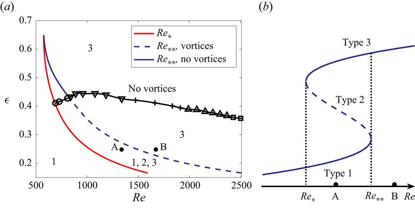
Figure 2. The existence map of azimuthally invariant steady solutions (a) and a schematic solution diagram for a fixed layer depth (b). Labels 1–3 in panel (a) correspond to the type 1–3 solutions, respectively. Robust free-surface vortex systems are only expected to exist to the right of the red line (for  ${{Re}}>{{Re}}_{*}$) and below the black line. The circles, down-pointing triangles, plus signs, upward-pointing triangles and squares correspond to systems with
  $m=4,\ldots,8$ vortices, respectively, that the base type 3 flow first bifurcates to as
  $\epsilon$ is decreased at constant
  ${{Re}}$. The region between the red and blue curves in panel (a) corresponds to the bistability interval
  ${{Re}}_{*}<{{Re}}<{{Re}}_{**}$ of azimuthally invariant states between the vertical dotted lines in panel (b).
To the left of the red curve  $\epsilon =\epsilon ({{Re}}_{*})$, a single steady-state solution referred to as type 1 exists. Three different kinds of flows termed types 1, 2 and 3 are found inside the crescent-shaped region between the red
  $\epsilon =\epsilon ({{Re}}_{*})$ and blue
  $\epsilon =\epsilon ({{Re}}_{**})$ lines. To the right of the blue line only the type 3 flow exists. This diagram in figure 2 is qualitatively similar to the axisymmetric steady flow existence map reported in Mullin & Blohm (Reference Mullin and Blohm2001) and Lopez, Marques & Shen (Reference Lopez, Marques and Shen2004) for Taylor–Couette-type flows arising in a short annular container mechanically driven by the co-rotation of the inner cylinder and the bottom end wall. However, there the cusp is formed by the saddle-node bifurcation curves corresponding to flow patterns
  $A_1$ and
  $A_3$ containing 1 and 3 meridional recirculation cells of approximately equal strength and aspect ratio 1 stacked vertically, respectively. This is different from the flow structures in our set-up, which we will detail below. Another difference is that here the cusp is formed as the electrolyte layer becomes deeper while in Lopez et al. (Reference Lopez, Marques and Shen2004) it appears as the annulus becomes shallower.
The type 1 flow computed for the parametric point A in figure 2 is illustrated in figure 3(a). It contains a single toroidal structure. The projection of its three-dimensional streamlines onto a meridional plane (referred to as meridional streamlines below) are shown in this figure. Schematically, this flow corresponds to the lower branch (solid line) in figure 2(b) (and to the  $A_1$ pattern in Lopez et al. Reference Lopez, Marques and Shen2004).

Figure 3. Meridional streamlines of the steady azimuthally invariant (a) type 1, (b) type 2, (d) type 3 solutions for  ${{Re}}=1337.95$ (point A in figure 2,
  ${{Re}}_{*}<{{Re}}<{{Re}}_{**}$) and (c) of the solution for
  ${{Re}}=1672.43$ (point B in figure 2,
  ${{Re}}>{{Re}}_{**}$) at
  $(\epsilon,{{{Ha}}})=(0.248,5.08\times 10^{-3})$. Colours represent the magnitude of the azimuthal velocity component
  $v$, the solid and dashed streamlines correspond to the clockwise and anticlockwise circulation, respectively. The fields in panels (a) and (b) are computed by Newton-type iterations, in panel (c) by the time integration starting from a motionless state and in panel (d) by the time integration starting from the field shown in panel (c).
The type 2 flow computed for the same values of the governing parameters is shown in figure 3(b). It has a different topology to the type 1 solution and contains the secondary toroidal structure in the corner between the outer vertical wall and the free surface of the electrolyte layer. This flow corresponds to the dashed line segment in figure 2(b) (its analog is not computed in Lopez et al. Reference Lopez, Marques and Shen2004). Both type 1 and 2 flows have been discussed in detail in Suslov et al. (Reference Suslov, Pérez-Barrera and Cuevas2017) and McCloughan & Suslov (Reference McCloughan and Suslov2020a). Thus, in the subsequent discussion we only recollect their most prominent features for the sake of comparison with those of the newly found flow state. In particular, our previous studies have shown that the type 1 flows are always linearly stable with respect to perturbations with any azimuthal wavenumbers, while type 2 flows are always unstable with respect to perturbations with wavenumbers  $m=0,1,\ldots,m_{max}$, where
  $m_{max}$ depends on
  ${{Re}}$ and
  $\epsilon$. The centrifugal instability of the type 2 steady azimuthally invariant flows has been argued to lead to the formation of anti-cyclonic vortices experimentally observed on the free surface of the layer (Pérez-Barrera et al. Reference Pérez-Barrera, Pérez-Espinoza, Ortiz, Ramos and Cuevas2015, Reference Pérez-Barrera, Ortiz and Cuevas2016, Reference Pérez-Barrera, Ramírez-Zúñiga, Grespan, Cuevas and del Río2019). However, the type 2 flow background on which such vortices could form has been found to exist only for a limited range of Reynolds number (or, equivalently, the electric current values)
  ${{Re}}_{*}<{{Re}}<{{Re}}_{**}$; see figure 2. Contradicting this finding experimental evidence exists that free-surface vortices appear over a much wider range of governing parameters to the right of the red curve
  $\epsilon =\epsilon ({{Re}}_{*})$ in figure 2(a). This strongly indicates that there should exist another steady or slowly evolving state that we refer to as the type 3 solution there with vortices forming on its background. Such a flow proved to be numerically quite elusive with a steady-state solver successfully used to obtain type 1 and 2 flows failing to converge for
  ${{Re}}>{{Re}}_{**}$, as was reported in McCloughan & Suslov (Reference McCloughan and Suslov2020a). The quadratic weakly nonlinear analysis developed there offered an explanation for this difficulty: it has been demonstrated that the type 1 and 2 flows undergo an ‘annihilating’ local saddle-node bifurcation at
  ${{Re}}_{**}$; see the ‘collision’ of the lower solid and middle dashed branches in figure 2(b) (and the
  $S_1$ line in Lopez et al. Reference Lopez, Marques and Shen2004). At the same time, the type 3 flow expected to exist for
  ${{Re}}\ge {{Re}}_{**}$ remains topologically ‘far away’ from both type 1 and 2 flows, which prevents using them as a starting point of a parametric continuation procedure aiming to locate the region of convergence for Newton-type iterations aiming to obtain the type 3 solution. To overcome such a difficulty, cubic nonlinear analysis has been performed in Part 1 (McCloughan & Suslov Reference McCloughan and Suslov2024) to construct an asymptotic solution past a saddle-node bifurcation point
  ${{Re}}_{**}$. It revealed that such a bifurcation in fact is a local feature of the global fold catastrophe, where the new solution of interest appears as a top branch labelled as type 3 in figure 2(b). Such an asymptotic solution for the parametric point B in figure 2 is illustrated in figure 11 in Part 1 (McCloughan & Suslov Reference McCloughan and Suslov2024). Although it was established in McCloughan & Suslov (Reference McCloughan and Suslov2020a) that type 2 flows lose the secondary toroidal structure responsible for the appearance of the anticyclonic free-surface vortices in the vicinity of
  ${{Re}}_{**}$ and become indistinguishable from the type 1 flows there, the asymptotic solution developed starting from it regains the secondary circulation; see figure 11 in Part 1 (McCloughan & Suslov Reference McCloughan and Suslov2024). This in turn strongly suggests that the ‘hunted’ type 3 flow would have to contain it as well, thus satisfying the necessary condition for the appearance of free-surface vortices. With this in mind, the obtained asymptotic solution was used as an initial guess for Newton iterations that finally converged to a steady state different from both type 1 and 2, thus, indeed demonstrating the existence of the type 3 azimuthally invariant flow.
Here we adopted an alternative numerical procedure to demonstrate the existence of the type 3 solution. We numerically integrate the  $\theta$-independent equations described in § 2 in time starting with a motionless initial state. For the parametric point A in figure 2, such a time integration recovered the steady type 1 flow shown in figure 3(a). This confirms that type 1 flows are always linearly stable and are topologically connected to the motionless state in the sense that they can be obtained via a parametric continuation starting with
  ${{Re}}=0$.
Performing a similar time integration of the  $\theta$-independent equations starting with a motionless state for the parametric point B in figure 2 (beyond the local saddle-node bifurcation) produced a steady state illustrated in figure 3(c). It is indistinguishable from that obtained by solving time-independent equations using Newton iterations and illustrated in figure 12 in Part 1 (McCloughan & Suslov Reference McCloughan and Suslov2024), thus validating both numerical procedures and showing that beyond the local saddle-node bifurcation point
  ${{Re}}_{**}$ there exists only one steady azimuthally invariant solution. It contains a secondary toroidal structure, which plays the main role in generating experimentally observable free-surface vortices. For
  ${{Re}}>{{Re}}_{**}$, such a structure evolves from an initial motionless state directly bypassing the type 2 flow state.
To confirm the conjecture of the fold catastrophe put forward based on the weakly nonlinear analysis arguments in Part 1 (McCloughan & Suslov Reference McCloughan and Suslov2024), we repeated time integration of the  $\theta$-independent equations for parameters corresponding to point A in figure 2 starting with the steady type 3 flow state found for point B in the same figure, that is from the field shown in figure 3(c). Such computations resulted in a steady state shown in figure 3(d). The comparison with type 1 and 2 flows depicted in figure 3(a,b) shows that the so-computed steady-state flow differs noticeably from them and, thus, represents another point on the type 3 solution branch. Parametric continuation from this point using a steady-state solver subsequently enabled us to trace the evolution of the new Type 3 solution over a wide range of the governing parameters. In particular, we confirmed that along with type 1 and 2 flow branches the type 3 solution forms a complete fold catastrophe as predicted in Part 1 (McCloughan & Suslov Reference McCloughan and Suslov2024) and schematically shown in figure 2(b) with a hysteresis being its most prominent feature (hysteresis is also found in Lopez et al. Reference Lopez, Marques and Shen2004).
While the time integration procedure has been developed primarily to obtain the analytically expected but numerically elusive type 3 flow solution, it enabled us to obtain valuable flow evolution data demonstrating the differences in the ways the topologically distinct steady flow states establish. In particular, figure 4 shows the families of azimuthal ( $v$) and radial (
 $u$) velocity components along the free surface for type 1 (figure 4a,c) and type 3 (figure 4b,d) flows traced from a motionless state. Both types of flows start developing near the inner cylinder when the driving current is switched on. Here the azimuthal motion arises first causing centrifugally forced radial flow. Combination of these two basic motions eventually leads to the establishment of toroidal flow structures, but in different ways for the two types of flow. The type 1 azimuthal velocity profile evolves monotonically outwards with the location of its maximum gradually moving from the inner to outer cylinder in the mid-term. At the final stages of the development its location stabilises but the magnitude continues to increase until it reaches the steady state. As a result, the steady type 1
  $v$ profile has a jet-like structure near the outer cylinder. The corresponding evolution of the radial velocity component
  $u$ is not monotonic. Initially, the fluid accelerates radially away from the inner cylinder with the maximum radial velocity component increasing with time. However, at later stages of the flow development this growth slows down and then reverses until the steady state is reached. At all times the radial velocity of the type 1 flow remains positive meaning that the fluid always flows towards the outer cylinder along the free surface.
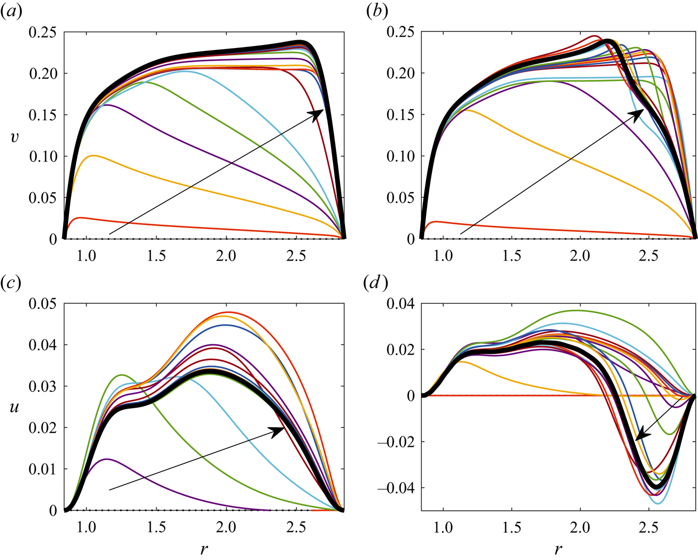
Figure 4. Temporal evolution from a motionless state of the free-surface azimuthal (a,b) and radial (c,d) velocity components of type 1 (a,c,  ${{Re}}=1377.95$) and type 3 (b,d,
  ${{Re}}=1672.43$) solutions at
  $(\epsilon,{{{Ha}}})=(0.248,5.08\times 10^{-3})$. The arrows indicate a general direction of the profile evolution. Thick black lines depict long-term steady-state velocity profiles.
Apart from the early stages of flow development, the temporal evolution of the type 3 flow shown in figure 4(b,d) is rather different. Neither azimuthal nor radial velocity components change monotonically. While initially the type 3 velocity profiles are qualitatively similar to those of type 1, at the final development stage they undergo a rapid modification. The  $v$ profile develops a prominent velocity deficit near the outer cylinder indicating noticeable deceleration of the overall flow at this location while the
  $u$ profile exhibits the reversal of the radial flow. As seen from figure 3(c,d) this corresponds to the appearance of a secondary counter-rotating toroidal structure near the corner between the free surface and the outer cylinder. As will be shown in § 3.2, the existence of such a structure determines the appearance of the anti-cyclonic vortices on the free surface.
3.2. Stability of the type 3 flows in a layer of fixed depth
Having established the topology of various azimuthally invariant steady flow types, next we investigate their linear stability with respect to small-amplitude perturbations characterised by the azimuthal wavenumber  $m=0,1,2\ldots$ (
 $m$ corresponds to the number of observable free-surface vortices). Such a stability investigation of type 1 and 2 flows has been reported in McCloughan & Suslov (Reference McCloughan and Suslov2020a). Therefore, here we focus on the type 3 flows and only mention the previously reported results for comparison and for completeness of discussion.
Figure 5 contains a comprehensive linear instability diagram of the type 3 flow. Different symbols correspond to growing modes with various wavenumbers. There are several important features distinguishing this map from its type 2 counterpart shown in figure 4(a) in McCloughan & Suslov (Reference McCloughan and Suslov2020a). In contrast to the type 2 flows, the number of modes with respect to which the type 3 flows become linearly unstable increases with Reynolds number (as the current driving the flow becomes stronger) and they continue to exist beyond the local saddle-node bifurcation that annihilates type 1 and 2 solutions. Given that free-surface vortices observed experimentally and reported in Pérez-Barrera et al. (Reference Pérez-Barrera, Pérez-Espinoza, Ortiz, Ramos and Cuevas2015) were detected for all current magnitudes larger than a certain value and would not disappear as the current was increased as long as the depth of the layer remained sufficiently small, we conclude that they are triggered by the instability of the type 3 rather than type 2 flows (the latter cease to exist for  ${{Re}}>{{Re}}_{**}$ while free-surface vortices are still visible for these Reynolds numbers). Moreover, now we can reasonably anticipate that even in the interval
  ${{Re}}_{*}<{{Re}}<{{Re}}_{**}$ the free-surface vortices develop on the background of the type 3 rather than type 2 azimuthally invariant flows. Indeed, computational results presented in McCloughan & Suslov (Reference McCloughan and Suslov2020a) demonstrated that the fastest growing linear instability mode for the type 2 flows corresponds to
  $m=0$, that is, to the
  $\theta$-independent mode; see upper half of the red curve in figure 6(a). Therefore, the
  $m=0$ mode is expected to modify the type 2 background flow quicker than the development time of azimuthally periodic modes with
  $m>0$ that can potentially give rise to the free-surface vortices but which have been computed under the assumption that the type 2 basic flow remains fixed and not affected by the
  $m=0$ instability mode. In contrast, the type 3 steady azimuthally invariant flow is found to be linearly stable with respect to the
  $m=0$ (and, in fact
  $m=1$) mode, see figures 5 and 6(a), with the fastest growing instability mode always corresponding to
  $m>1$. This observation suggests that, depending on the initial conditions, the free-surface vortex onset process may consist of two consecutive stages. Initially, the overall flow develops towards the azimuthally invariant type 2 state. However, this state is unstable with respect to the
  $\theta$-independent perturbations. While free-surface vortices may start developing at this stage, the evolution of type 2 flow towards its type 3 counterpart is expected to happen faster so that in the longer term free-surface vortices would continue to develop on the type 3 background. An alternative scenario could be that the type 2 flow evolves towards the type 1 counterpart. In that case the free-surface vortices would eventually disappear. Therefore, the linear stability analysis indicates that the type 2 states being unstable with respect to the
  $m=0$ mode may belong to the boundary between the basins of attraction of type 1 and type 3 flows as indicated by the dashed line in the schematic diagram of figure 2(b). As such, experimentally they could be observed only as transient states in a bistable system, where the two long-term states differ by the presence or absence of the free-surface vortices for the same set of governing parameters. Such a bistability regime is expected to exist in an electrolyte layer of a fixed depth only for
  ${{Re}}_{*}<{{Re}}<{{Re}}_{**}$. For
  ${{Re}}<{{Re}}_{*}$, no free-surface vortices exist while, for
  ${{Re}}>{{Re}}_{**}$, they are expected to always develop.
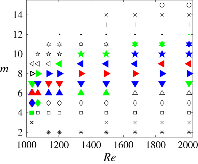
Figure 5. Linear instability diagram for the type 3 flow in the  $h=7.5$ mm-deep electrolyte layer
  $(\epsilon =0.248)$ placed 6 mm above the vertically polarised disk magnet with
  $B_0=0.02$ T. Symbols show wavenumbers of linearly unstable modes. The red symbols correspond to the wavenumbers of the most amplified instability modes, the blue and green symbols mark modes with amplification rates within 10 % and 20 % of the maximum, respectively.
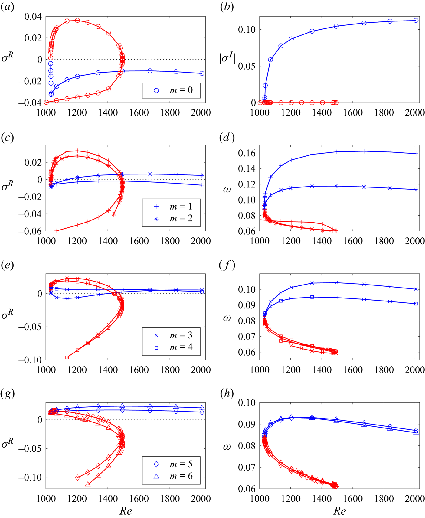
Figure 6. The largest linear amplification growth rates  $\sigma ^R$ (a,c,e,g) and the corresponding oscillation frequencies
  $|\sigma ^I|$ (
 $m=0$) and angular speeds
  $\omega =-\sigma ^I/m$ (
 $m\ne 0$) of the vortex translation (b,d,f,h) for the stability diagram shown in figure 5. The lower
  $(\sigma ^R<0)$ and upper
  $(\sigma ^R>0)$ branches of the red curves in (a,c,e,g) correspond to the previously investigated (McCloughan & Suslov Reference McCloughan and Suslov2020a, figure 5) type 1 and 2 solutions, respectively, the blue curves denote values obtained for the newly discovered type 3 flow.
The red, blue and green symbols in figure 5 correspond to modes with the maximum linear amplification rates, and with growth rates that are within 10 % and 20 % of the maximum, respectively. As seen from the figure, for all Reynolds numbers, the spectrum of fastest growing modes is sufficiently wide and includes up to five modes that are expected to interact with each other as they develop. The fact that the most amplified modes have very close angular wave speeds  $\omega =-\sigma ^I/m$, see figures 6(b,d,f,h) and 7(b,d,f), speaks strongly in favour of this conjecture as well. It is impossible to determine details of such an interaction and mode selection mechanism within a linear stability consideration alone. Further investigation of this aspect requires a weakly nonlinear coupling analysis that, given its length and algebraic complexity, we plan to report in a separate publication. Here we only mention that experimental observations reported in Pérez-Barrera et al. (Reference Pérez-Barrera, Pérez-Espinoza, Ortiz, Ramos and Cuevas2015, Reference Pérez-Barrera, Ortiz and Cuevas2016) indicate that the number of observable free-surface vortices can change with time. This could be caused by both the transition from the type 2 to type 3 azimuthally invariant background flow and the interaction between several instability modes. Such a mode competition scenario has also been studied, for example, in Lopez & Marques (Reference Lopez and Marques2004) for cylindrical flows driven by co-rotating end walls, although the number of competing rotating wave modes found there was only two. In this regard, the situation encountered here appears to be closer to that of multiple wall-mode competition in rotating Rayleigh–Bénard convection discussed, for example, in Lopez et al. (Reference Lopez, Marques, Mercader and Batiste2007), where a Benjamin–Feir secondary instability mechanism has been found responsible for the mode selection.
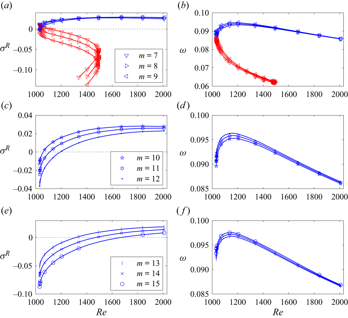
Figure 7. The same as figure 6 but for larger wavenumbers. The growth rate and angular speed curves for type 1 and 2 flows are not shown for  $m>9$ since the perturbation modes with these wavenumbers are found to always decay.
Figures 6 and 7 offer further insight into the transition between the type 2 and 3 flows occurring at  ${{Re}}_{*}$. The corresponding red and blue curves join in a continuous way similar to the way the curve branches corresponding to type 1 and 2 flows meet at
  ${{Re}}_{**}$ (the right extreme of the red curves in these figures). This demonstrates that at
  ${{Re}}_{*}$ the type 2 and 3 flows morph into each other in a continuous way and undergo a local saddle-node bifurcation similar to that discussed in McCloughan & Suslov (Reference McCloughan and Suslov2020a). Therefore, our present numerical stability results fully confirm the conclusion made in Part 1 (McCloughan & Suslov Reference McCloughan and Suslov2024) based on weakly nonlinear considerations that type 1, 2 and 3 flows form branches of a classical fold catastrophe illustrated in figure 2(b) with the two local saddle-node bifurcations occurring at its turning points that we now refer to as fold points.
Further inspection of figure 6(a,b) reveals more noteworthy details of azimuthally invariant perturbation modes. At the fold point  ${{Re}}={{Re}}_{*}$ the merging type 2 and type 3 flows are neutrally stable with respect to them, and the
  $m=0$ modes are non-oscillatory there. Away from the fold point (for
  ${{Re}}>{{Re}}_{*}$) the
  $m=0$ mode remains non-oscillatory but becomes destabilising for the type 2 flow. In contrast, a similar mode for the type 3 flow is characterised by a steeply increasing decay rate and becomes oscillatory. Such a behaviour is clarified in figure 8, where three leading eigenvalues
  $\sigma$ computed for
  $m=0$ are shown as functions of
  ${{Re}}$ in the vicinity of
  ${{Re}}_{*}$. The linear stability investigation reveals that near
  ${{Re}}_{*}$ multiple perturbation modes have close growth rates; see figure 8(a). The corresponding eigenvalues experience multiple bifurcations (‘collide’) as
  ${{Re}}$ increases so that, as a result, the mode with the smallest decay rate (the red curve) changes its nature from monotonic to oscillatory at
  ${{Re}}\approx 1034$. This has a direct influence on the temporal evolution of the type 3 flow as is evidenced by the velocity time series computed for the same parameters as in figure 3(c,d) for the point shown by the black circle in panel (d) there. After the initial transient, the local flow evolution within the secondary circulation cell obtained by time integration of the
  $\theta$-independent governing equations takes the form of exponentially decaying oscillations with non-dimensional frequencies
  $\nu \approx 1.083\times 10^{-1}$ (the left column in figure 9) and
  $\nu \approx 9.82\times 10^{-2}$ (the right column in figure 9). These are in excellent agreement with the corresponding values of
  $|\sigma ^I|\approx 1.088\times 10^{-1}$ and
  $|\sigma ^I|\approx 9.76\times 10^{-2}$ obtained from the linear stability computations for infinitesimal perturbations. The inspection of the numerically obtained time-dependent type 3 flow fields (not shown here) reveals that such decaying oscillations involve a precession of the secondary circulation cell around its azimuthal axis with a periodic variation of its shape until it settles to that shown in figure 3(c,d).
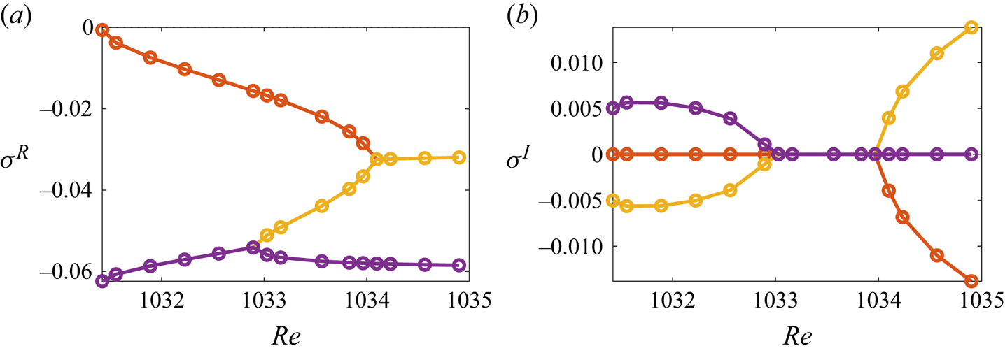
Figure 8. The real and imaginary parts of the three leading eigenvalues corresponding to the  $m=0$ perturbation modes computed for the type 3 flow for the values of
  ${{Re}}$ in the vicinity of the fold point
  ${{Re}}_{*}$ at
  $\epsilon =0.248$.
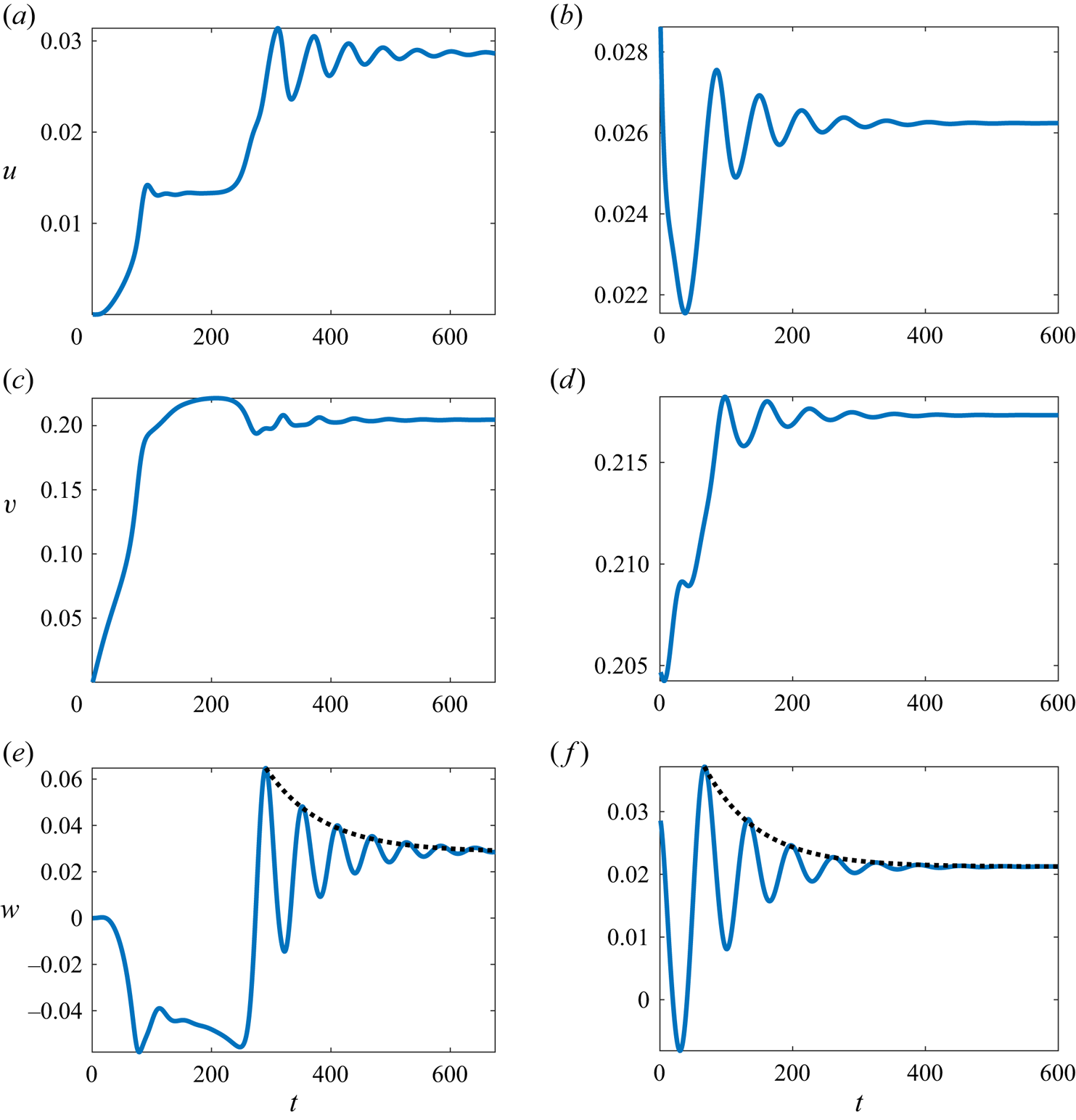
Figure 9. Temporal evolution of the flow velocity components at the point shown by the black circle in figure 3(d). Time integration is performed from a motionless state for  $({{Re}},\epsilon,{{{Ha}}})=(1672.43,0.248,5.08\times 10^{-3})$ (a,c,e) and starting with the steady-state field shown in figure 3(c) for
  $({{Re}},\epsilon,{{{Ha}}})=(1337.95,0.248,5.08\times 10^{-3})$. The dotted lines in panels (e,f) show exponential decay
  $\sim \exp (\sigma ^Rt)$, where the decay rates
  $\sigma ^R=-1.05\times 10^{-2}$ (a,c,e) and
  $\sigma ^R=-1.23\times 10^{-2}$ (b,d,f) are determined from linear stability analysis.
Having established the nature of the background  $\theta$-independent flows and their temporal evolution towards a steady state, we are now in a position to discuss the most prominent experimentally observable (Pérez-Barrera et al. Reference Pérez-Barrera, Pérez-Espinoza, Ortiz, Ramos and Cuevas2015, Reference Pérez-Barrera, Ortiz and Cuevas2016; Suslov et al. Reference Suslov, Pérez-Barrera and Cuevas2017) feature of the electrolyte flow driven by the Lorentz force in an annular channel: the free-surface vortices. To do that, we refer to figure 10 where the typical perturbation streamlines and vertical vorticity field occurring on the type 3 flow background at the free surface are shown for the linearly most amplified disturbance mode. This example corresponds to wavenumber
  $m=8$. To avoid potential confusion with a 16-cell structure visible in the figure, we note that in reality such a pattern would occur on a background of the main cyclonic motion that would have its own vertical component of vorticity. It would have a definite sign at the location of the perturbation structures. For example, if the main motion occurs in the anticlockwise direction, the background vertical vorticity component near the outer cylindrical wall is negative due to the influence of the viscous boundary layer there. Therefore, when the perturbation vorticity is added to the background one, the periodic cells with positive vertical vorticity would be weakened while those with negative vorticity would be amplified. Thus, in experiments one would only see eight well pronounced anti-cyclonic (rotating clockwise in the chosen example) vortices ‘rolling along’ the outer wall in the direction of the main flow as indeed shown in figure 1 in Suslov et al. (Reference Suslov, Pérez-Barrera and Cuevas2017). This qualitative discussion explains why wavenumber
  $m$ indeed represents the number of experimentally visible vortices even though reconstructing the full picture using only the knowledge of the background flow and the spatial form of an eigenfunction is impossible since its amplitude cannot be determined within the framework of a linear stability analysis.
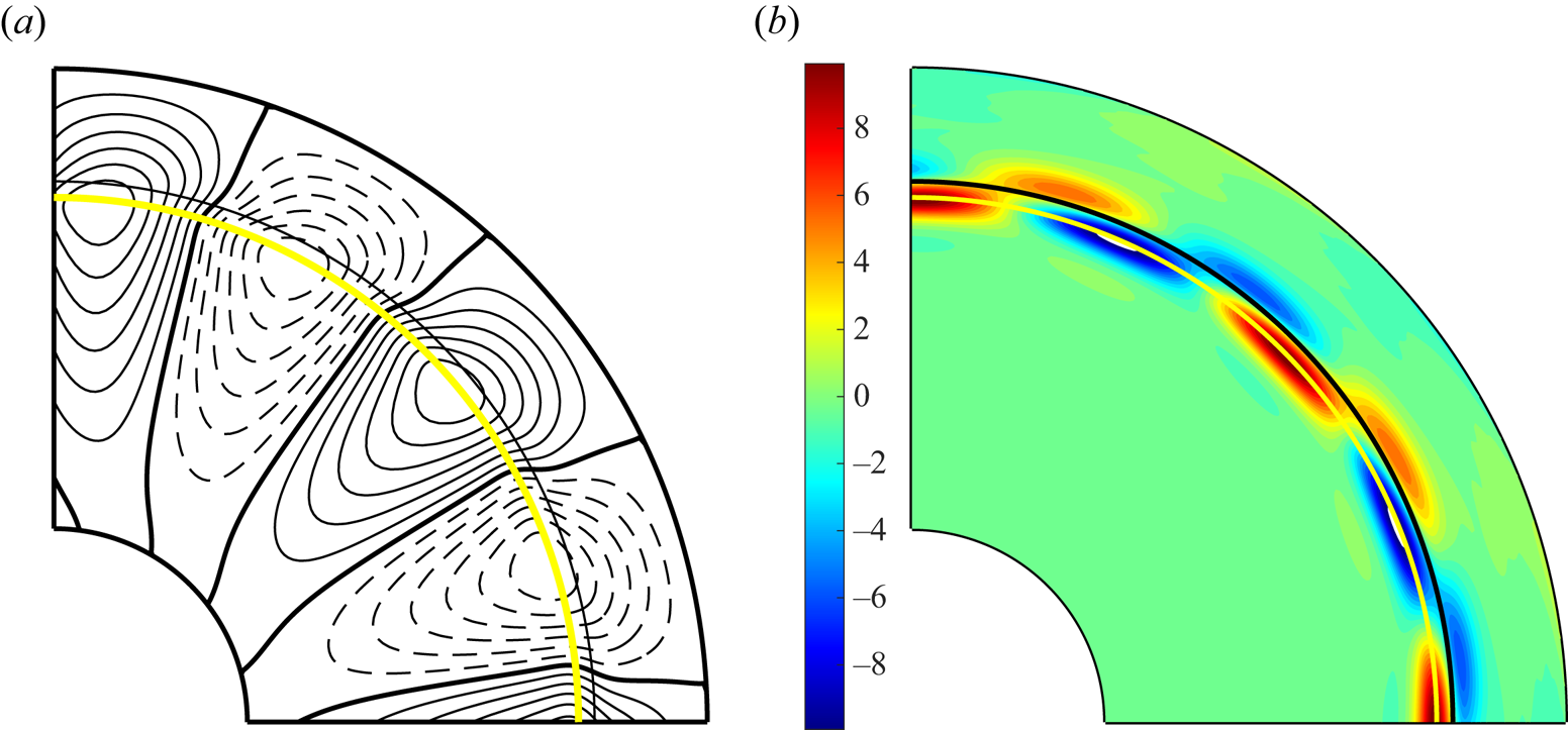
Figure 10. Instantaneous perturbation streamlines  $\boldsymbol {u}'$ (a) and the vertical perturbation vorticity
  $\omega '_z=D_rv'+v'/r$ (b) field at the free surface (
 $z=1$) for the fastest growing instability mode (
 $m=8$) developing on the type 3 basic flow background for the same parameters as in figure 3(d) (arbitrary colour scale). The yellow quarter circles mark the locations
  $r_l$ on the free surface, where the radial and vertical basic flow velocity components
  $\bar u=\bar w=0$, while the azimuthal component
  $\bar v\ne 0$ (see figure 3d). It separates the main and secondary toroidal flow structures. The black quarter circles show the locations, where the free-surface azimuthal velocity
  $\bar v$ is equal to the perturbation wave speed
  $v_c=\omega r$.
The yellow and black quarter circles in figure 10 show the locations along the free surface, where the radial velocity component  $u=0$ and where the free-surface azimuthal velocity component
  $v=v_c$, where
  $v_c=\omega r=-(\sigma ^Ir)/m$ is the local linear perturbation wave speed, respectively. The
  $u=0$ (yellow) line may be viewed as the projection of the boundary of the secondary toroidal structure present in the type 3 flows onto the free surface. It is seen that an instability pattern responsible for the formation of the experimentally observed free-surface vortices is strongly localised near such a boundary, see also figure 11, where the meridional structure of the perturbation fields is shown. The
  $v=v_c$ quarter circle passes through the middle of the instability pattern demonstrating that the so-generated vortex system is essentially ‘carried’ by the background type 3 azimuthal flow. The same conclusion was made in McCloughan & Suslov (Reference McCloughan and Suslov2020a) regarding the location and motion of instabilities of the type 2 flows. The perturbation energy analysis presented there for the type 2 flows identified the physical nature of their instabilities as centrifugal (Rayleigh type). A similar analysis that we completed for instabilities of the type 3 flows shows that they are also of the centrifugal type but, for brevity, we leave the algebraic and computational details of this investigation outside the current paper. Instead, here we follow Billant & Gallaire (Reference Billant and Gallaire2005) to confirm the centrifugal nature of the observed instability from a different point of view.
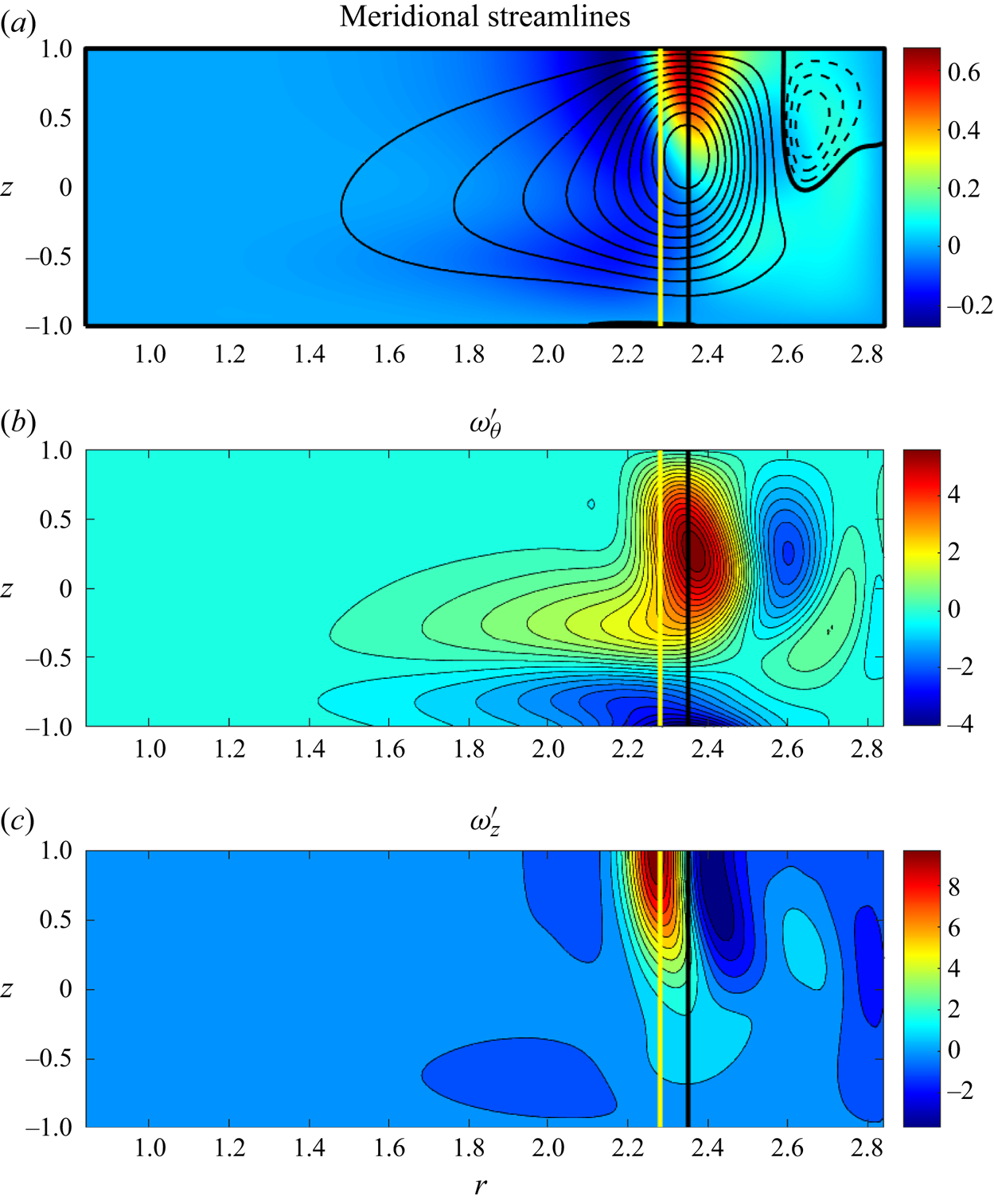
Figure 11. The instantaneous perturbation streamlines (a) and azimuthal (b) and vertical (c) vorticity fields for the fastest growing instability mode ( $m=8$) in the meridional plane
  $\theta =0$ for the same parameters as in figure 3(d) (arbitrary colour range scaling). In panel (a) the colour represents the azimuthal perturbation velocity component. The yellow and black vertical lines correspond to the respective quarter circles in figure 10.
The meridional cross-sections of the perturbation velocity and vorticity fields illustrated in figure 11 show that the observed free-surface vortices formed on the type 3 basic flow background are rather shallow. Similar to those reported in McCloughan & Suslov (Reference McCloughan and Suslov2020a) for the type 2 background, they occupy less than a half of the total fluid layer depth. In view of this, we consider a somewhat crude approximation of the type 3 background flow that nevertheless provides a qualitatively correct interpretation of the arising instability. Namely, given a small vertical extent of the observable vortices and the fact that near the free surface and in the vicinity of the boundary separating the two toroidal structures forming the type 3 flow  $u\approx w\approx 0$, the flow there is essentially circumferential and similar to that of free vortices. If in addition the fluid viscosity is neglected, such vortices may be subject to Rayleigh centrifugal instability with respect to azimuthally invariant (Rayleigh Reference Rayleigh1917; Greenspan Reference Greenspan1968) or periodic perturbations with the azimuthal wavenumber
  $m>0$.
The inviscid instability criterion is formulated in terms of the angular velocity  $\varOmega ={v}/{r}$ and the Rayleigh discriminant
  $\varphi =({1}/{r^4})\partial _r(r^4\varOmega ^2)$. The example of their radial distribution along the free surface in the type 3 flow is shown in figure 12. As derived in Billant & Gallaire (Reference Billant and Gallaire2005), the complex growth rate of azimuthally
  $m$-periodic infinitesimal perturbations is given by
 \begin{equation} \sigma_m(r_0)=-{\rm i} m \varOmega(r_0)+\sqrt{-\varphi(r_0)}, \end{equation}
where (potentially complex valued)  $r_0$ is the point where
  $\partial _r\sigma _m(r)=0$. If
  $m=0$ then the growth rate is real and positive, that is, the centrifugal instability is present provided that
  $\varphi$ has a negative minimum at
  $r_0$, which is indeed evident from figure 12(b).
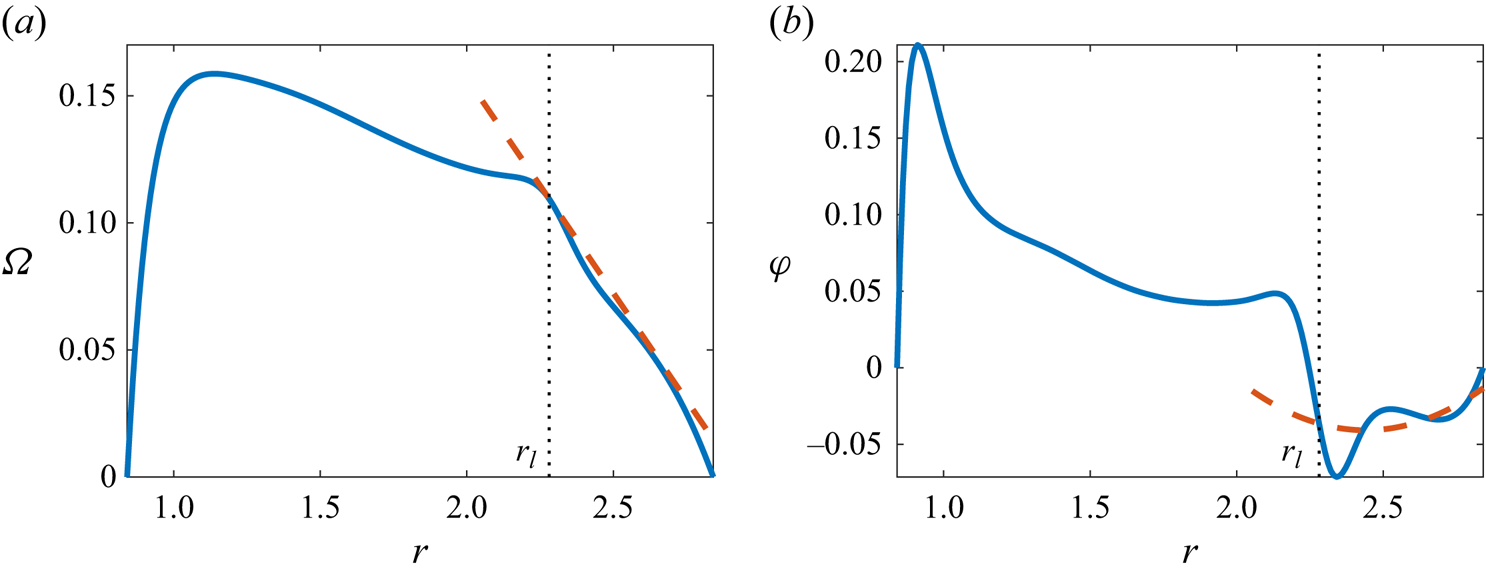
Figure 12. Free-surface angular speed  $\varOmega ={v}/{r}$ (a) and Rayleigh discriminant
  $\varphi =({1}/{r^4})\partial _r(r^4\varOmega ^2)$ for the type 3 flow for the same parameters as in figure 3(a). The vertical dotted line corresponds to the radial location
  $r_l=2.28$ on the free surface, where
  $u=w=0$ (the yellow quarter circle in figure 10). The dashed lines correspond to a linear local approximation of the angular speed distribution
  $\varOmega \approx \omega _l-a(r-r_l)$, where
  $\omega _l={v(r_l,1)}/{r_l}=0.11$ and
  $a=0.17$.
To assess the possibility of centrifugal instability in the form of azimuthally  $m$-periodic perturbations, we note that within the secondary circulation structure of the type 3 flow (to the right of the dashed vertical line
  $r=r_l$, where
  $u=w=0$, in figure 12) the distribution of the angular speed is close to linear so that
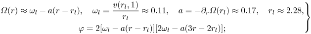 \begin{align} \left. \begin{gathered} \varOmega(r)\approx\omega_l-a(r-r_l),\quad \omega_l=\dfrac{v(r_l,1)}{r_l}\approx0.11,\quad a=-\partial_r\varOmega(r_l)\approx0.17,\quad r_l\approx2.28,\\ \varphi=2[\omega_l-a(r-r_l)][2\omega_l-a(3r-2r_l)]; \end{gathered} \right\} \end{align}
see the dashed lines. We use these approximations to estimate the growth rates associated with the centrifugal instability. Similar to Billant & Gallaire (Reference Billant and Gallaire2005) we find that, for  $m\ne 0$,
  $r_0$ is a double turning point given by
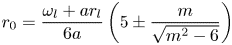 \begin{equation} r_0=\frac{\omega_l+ar_l}{6a}\left(5\pm\frac{m}{\sqrt{m^2-6}}\right) \end{equation}
so that
 \begin{equation} \sigma_{m1} =\frac{\omega_l+ar_l}{6}\left(\dfrac{6+m^2}{\sqrt{6-m^2}} -{\rm i} m\right),\quad \sigma_{m2} =\frac{\omega_l+ar_l}{6}\left(\sqrt{6-m^2}-{\rm i} m\right). \end{equation}
In the large wavenumber limit the above expressions become
 \begin{align} \sigma_{m1}=-{\rm i}\frac{\omega_l+ar_l}{6}\left(2m+\frac{9}{m} +O\left(m^{-3}\right)\right),\quad \sigma_{m2}=-{\rm i}\frac{\omega_l+ar_l}{2m} +O\left(m^{-3}\right). \end{align}
 Even though the above expressions are obtained using a very crude approximation (neglecting the radial and vertical velocity components and the dissipation due to viscous shear), they enable a number of qualitative observations that are consistent with our computational stability results. Firstly, the real part of the estimated perturbation amplification rate is positive only for wavenumbers  $m=0$, 1 and 2, with
  $m=2$ being the fastest growing inviscid centrifugal mode. Figure 6 indeed demonstrates that the largest growth rates computed for these wavenumbers increase from
  $m=0$ to
  $m=2$. Figure 6 also shows that, for
  $m>2$, the qualitative behaviour of the amplification rate curves changes compared with that of the
  $m\le 2$ modes. This is consistent with the fact that expression (3.4a,b) becomes purely imaginary for
  $m>2$ indicating that all subsequent inviscid modes are neutrally stable so that other factors (viscous effects, three-dimensionality of the velocity field) that are neglected in this expression dictate whether the instability in the form of large-wavenumber modes occurs. Furthermore, as follows from the expression (3.5a) for large
  $m$, the angular speed of perturbations tends to the value
  $\omega _m=\textrm {i}({\sigma _{m1}}/{m})=({\omega _l+ar_l})/{3}$ that is independent of the wavenumber, which is indeed what figure 7 shows.
Having confirmed that the appearance of the free-surface vortices is closely linked to the existence of a secondary toroidal structure in the background flow, it is of interest to investigate how such an instability is affected by the size of this structure, which we define as the non-dimensional radial distance  $l=1+\alpha -r_l$ from the outer cylinder to the
  $u(r_l,1)=0$ line (yellow quarter circle) on the free surface. Figure 13(a) demonstrates that the characteristic size of the secondary circulation cell monotonically increases with the applied Lorentz forcing characterised by the value of
  ${{Re}}$. As a result, the boundary separating the two counter-rotating toroidal structures in the type 3 flow moves away from the outer cylindrical wall and the angular speed of the background type 3 flow there starts decreasing after reaching a maximum at lower values of
  ${{Re}}$; see figure 13(b). This explains a similar behaviour of the angular wave speed of the observable free-surface vortices shown in figures 6(b,d,f,h) and 7(b,d,f): despite strengthening of the Lorentz force driving the background flow, the propagation speed of vortices that follow the local flow decreases after reaching the maximum.
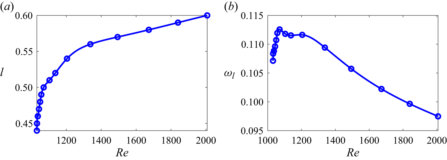
Figure 13. The meridional size  $l=\alpha +1-r_l$ of the secondary circulation cell (a) and the angular free-surface speed
  $\omega _l$ (b) as functions of the Reynolds number for
  $(\epsilon,{{{Ha}}})=(0.248,5.08\times 10^{-3})$. The quantities
  $r_l$ and
  $\omega _l$ are defined in figure 12.
The other important consequence of the fact that the boundary of the secondary circulation cell moves towards the inner cylinder, where the azimuthal fluid speed is lower, as the Lorentz force increases is that the centrifugal effects weaken there. As the result, the necessary condition for the formation of free-surface vortices cannot be satisfied anymore and the linear stability analysis predicts their disappearance. Thus, we observe a somewhat counter-intuitive effect: despite increasing forcing and a higher rotation speed of the base flow, the vortex existence region in the  $({{Re}},\epsilon )$ parametric space becomes smaller at larger
  ${{Re}}$, as indeed shown by the sloping down solid black line in figure 2(a).
3.3. Variation of the free-surface vortex patterns with the fluid layer depth
So far, our discussion has been limited to physical trends observed as the driving Lorentz force varies while the fluid layer depth remains fixed (all numerical results have been presented along a horizontal line passing through points A and B in figure 2(a). Experimentally, this would correspond to changing the strength of the total radial current flowing through the electrolyte between cylindrical electrodes. At smaller electrolyte depths the relative role of viscous dissipation at the bottom of the layer increases. Consequently, while the overall qualitative structure of the flow is preserved, it takes a larger current to drive it. This is seen in figure 2(a): the boundaries of the bistability region curve towards higher values of  ${{Re}}$. The corresponding fast flows in thin layers would necessarily lead to a noticeable deviation of the free surface from horizontal, which in turn would make the currently used numerical approximation based on the flat-surface assumption (Satijn et al. Reference Satijn, Cense, Verzicco, Clercx and van Heijst2001; Delacroix & Davoust Reference Delacroix and Davoust2014) quantitatively inaccurate. For this reason, we limit our current computations to
  $\epsilon >0.1$. Despite this limitation, our results confirm the experimentally observed trend (Pérez-Barrera et al. Reference Pérez-Barrera, Pérez-Espinoza, Ortiz, Ramos and Cuevas2015, Reference Pérez-Barrera, Ortiz and Cuevas2016) that in thinner layers the number of observable vortices is larger. We have found that, for the decreasing values of
  $\epsilon$, the wavenumber corresponding to the most amplified linear instability mode of the type 3 flow increases in a similar way to that demonstrated in McCloughan & Suslov (Reference McCloughan and Suslov2020a, figure 4b) for the type 2 flow.
In thicker layers this trend is reversed: the wavenumber of the most unstable mode decreases and the overall wavenumber range of unstable modes narrows. Eventually, only one unstable mode remains that is created as a result of Hopf bifurcation from the type 3 azimuthally invariant steady flow. The locations of such Hopf bifurcations are shown by the black line in figure 2(a). The wavenumber  $m$ at bifurcation points increases from 4 at the fold-Hopf point
  $({{Re}}_{*},\epsilon )\approx (691.3,0.411)$ to 8 near the right edge of the figure as
  ${{Re}}$ increases, as shown by various symbols in figure 2(a), and no vortices are expected to exist for the values of
  $\epsilon$ above the black line. The location along this line, where the wavenumber changes from
  $m$ to
  $m+1$ corresponds to codimension-2 Hopf bifurcations, where the growth rates of the two spectrally adjacent modes are zero. The presence of a similar sequence of codimension-2 points was also detected, for example, in a flow within a rotating-lid cylinder (Gelfgat, Bar-Yoseph & Solan Reference Gelfgat, Bar-Yoseph and Solan2001). The unfoldings of selected codimension-2 points existing in Taylor–Couette flows in a finite-aspect-ratio cylinder with stationary end and outer walls demonstrating a very rich dynamics has been considered by Abshagen et al. (Reference Abshagen, Lopez, Marques and Pfister2005) and Lopez & Marques (Reference Lopez and Marques2005).
A possible physical reason why in thicker layers the range of wavenumbers of unstable modes narrows is that the characteristic size  $l$ of the secondary circulation cell increases noticeably as the layer depth increases (see figure 15 discussed below) so that the boundary separating it from the primary toroidal structure, where free-surface vortices occur, shifts towards the axis of the annular channel. Congestion caused by the decreasing circumference over which the vortices are placed leads to the decrease of their number.
The enlargement of the secondary toroidal structure in thicker layers has another, perhaps, more profound effect. As is the case with  ${{Re}}$ increasing at constant
  $\epsilon$, the location, where the free-surface vortices can potentially arise, shifts towards smaller values of the radial coordinate
  $r$, where the centrifugal effects that are responsible for the vortex creation weaken. Eventually, they become insufficient to overcome viscous dissipation strengthened by the circumferential congestion, and the type 3 flows linearly completely stabilise at
  $\epsilon \approx 0.444$ (
 $h=13.4$ mm). Figure 14 confirms that the linear instability growth rates
  $\sigma ^R$ remain non-positive for all wavenumbers with
  $m=5$ predicted to be the last surviving free-surface vortex system. Therefore, our analysis predicts that in thicker layers (
 $\epsilon \gtrsim 0.444$) the free-surface vortices may appear only transiently if the type 2 background flow can be temporarily induced (recollect that the azimuthally invariant type 2 flows are shown to be unstable and undergo transition to either type 1 or 3 flows).
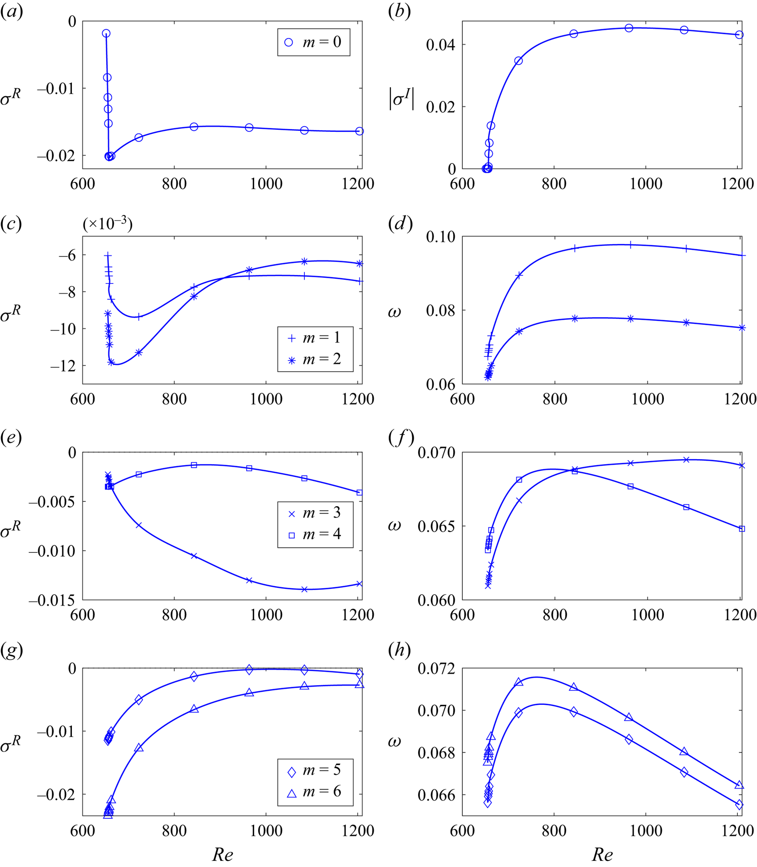
Figure 14. The largest linear amplification growth rate  $\sigma ^R$ (a,c,e,g) and the oscillation frequency
  $|\sigma ^I|$ (
 $m=0$) and the angular speed
  $\omega =-\sigma ^I/m$ (
 $m\ne 0$) of the vortex translation (b,d,f,h) for the type 3 flow in the 13.5 mm-deep electrolyte layer
  $(\epsilon =0.477)$.
Finally, the analysis presented in Part 1 (McCloughan & Suslov Reference McCloughan and Suslov2024) demonstrated that at  $({{Re}},\epsilon )\approx (577.05,0.649)$ (the top tip of the crescent-shaped bistability region in figure 2a) the background flow experiences a cusp catastrophe in which the type 2 flow completely disappears and the type 1 flow existing at small Reynolds numbers transitions directly to the type 3 flow as
  ${{Re}}$ increases; see figure 15. No free-surface vortices are expected to be observable in such regimes in the long term given that both the type 1 and 3 background flows remain linearly stable and the type 2 flows cannot exist.
Figure 15. Meridional streamlines for flow fields computed using Newton-type iterations with parametric continuation for  $(\epsilon,{{{Ha}}})=(0.662,1.35\times 10^{-2})$ and (a)
  ${{Re}}=428$, (b)
  ${{Re}}=482$, (c)
  ${{Re}}=535$ and (d)
  ${{Re}}=589$. Colours represent the magnitude of the azimuthal velocity component
  $v$, the solid and dashed streamlines correspond to the clockwise and anticlockwise circulation, respectively.
4. Notes on the robustness and completeness of the reported results
While the analytical and computational results that we have reported in this and a series of our previous publications (Suslov et al. Reference Suslov, Pérez-Barrera and Cuevas2017; McCloughan & Suslov Reference McCloughan and Suslov2020a,Reference McCloughan and Suslovb, Reference McCloughan and Suslov2024) represent a comprehensive study of extremely rich flow regimes existing in a simple geometry of an annular channel that makes them easily accessible to an experimental verification, several points have to be mentioned regarding potential ambiguities one may encounter.
Firstly, as mentioned in the previous section, care must be taken of the shape of the free surface. In experiments it is necessarily curved with the highest point located near the outer cylinder. In all our computations this deformation has been estimated (Suslov et al. Reference Suslov, Pérez-Barrera and Cuevas2017) not to exceed a few percent of the average layer thickness and, thus, has been neglected. In very thin layers though this might not be the case and experiments might reveal additional flow features (for example, a centrifugal rapture of thin electrolyte layers that might lead to the appearance of radial waves and sloshing) not captured by the current analysis.
Secondly, the geometry and dimensions of the considered flow domain have been suggested by experiments reported in Pérez-Barrera et al. (Reference Pérez-Barrera, Pérez-Espinoza, Ortiz, Ramos and Cuevas2015, Reference Pérez-Barrera, Ortiz and Cuevas2016). Thus, the average non-dimensional channel radius  $\alpha$ has been fixed in all our computations. It is not expected that the qualitative flow trends would change if experiments are conducted in an annulus of a somewhat different curvature, but given that the mechanism triggering the appearance of the free-surface vortices is of the centrifugal nature, quantitative characteristics of the observed vortex systems are likely to differ from those reported here even if the channel aspect ratio
  $\epsilon$ is chosen to be the same as in our studies.
Thirdly, for weakly conducting electrolyte flows characterised by small  $(O(10^{-3}))$ values of Hartmann number, the main flow characteristics are fully determined by the geometric parameters
  $\alpha$ (fixed in all our studies) and
  $\epsilon$ (varied in our investigation) and the Reynolds number
  ${{Re}}$ (also varied) effectively characterising the strength of the driving Lorentz force. This reflects the fact that while the background flow in the considered set-up is driven electromagnetically, the observed instabilities are found to be of a pure hydrodynamic nature. However, if experiments are conducted with better conducting fluids (e.g. concentrated electrolytes or liquid metals), the results are expected to be also affected by the variation of Hartmann number that characterises the variation of electric potential within the electrolyte layer caused by the flow of electrically conducting fluid.
Fourthly, in all our computations we used the same axisymmetric spatial distribution of the applied magnetic field as in Suslov et al. (Reference Suslov, Pérez-Barrera and Cuevas2017). It was computed under the assumption that an ideal vertically polarised permanent disk magnet was placed a distance  $d=6$ mm under the lower edge of the electrolyte layer (
 $d$ is the thickness of the bottom wall of an experimental channel). Measuring a realistic magnetic field in experiments is a rather complicated procedure prone to various inaccuracies. Therefore, while it is possible to accurately recreate the geometric configuration of the flow channel used in our studies, it is unlikely that one can match identically the distribution of a magnetic field used in our analysis. However, we note that the magnetic field used in earlier experiments of Pérez-Barrera et al. (Reference Pérez-Barrera, Pérez-Espinoza, Ortiz, Ramos and Cuevas2015, Reference Pérez-Barrera, Ortiz and Cuevas2016) was created not by a disk-shaped, but a rectangular magnet so that its magnetic field was not axisymmetric. Yet, the flow patterns observed in an annular electrolyte layer were found to be very similar to those we report here for an idealised axisymmetric field. The physical reason for this is that weakly conducting fluids experience a Lorentz force that is primarily defined by the vertical component of the magnetic field, while the field asymmetry is mostly created by the magnet edge effects causing the non-uniformity of horizontal field components. Therefore, the shape of the magnet used in experiments is not expected to have a strong influence on the observed flows as long as the magnet is vertically polarised and its horizontal dimensions are larger than the diameter of the experimental flow domain.
Fifthly, when an electric current flows through an electrolyte, it inevitably causes electrolysis on the electrodes forming the side walls of the channel. This leads to the formation of gas bubbles on the side surfaces. They may disrupt the no-slip boundary assumption used in our analysis. This is expected to lead to a difference between experimentally observed and computed flows, which is likely to become noticeable for thin layers, where the size of the formed bubbles could be comparable with the depth of the layer. However, such bubbles usually require a longer time to grow than the characteristic flow development time. Therefore, the flow features that we predicted in our analytic and numerical studies should still be possible to detect even in experiments with sufficiently thin electrolyte layers.
Finally, we note that several aspects of the flow dynamics could not be assessed by means of analytic and numerical tools described here. In particular, it is found that several instability modes with a different number of free-surface vortices can have very close linear growth rates and wave speeds and it is not clear how the dominant mode is selected. The details of a likely interaction between various vortex instability modes also remain undetermined. We plan to investigate these aspects using weakly nonlinear analysis and fully three-dimensional direct numerical simulations and report results in a separate publication.
5. Conclusions
In this paper we continued to study a rich variety of flows occurring in an annular electrolyte layer placed in an external magnetic field and carrying a radial electric current. The arising Lorentz force drives the azimuthal motion of the fluid that is shown to experience centrifugal instability leading to the appearance of experimentally observable systems of free-surface vortices. Part 1 of this study (McCloughan & Suslov Reference McCloughan and Suslov2024) focused on the asymptotic weakly nonlinear analysis of steady azimuthally invariant flows. It revealed that they undergo a hierarchy of transitions between multiple solutions via a saddle-node bifurcation and fold and cusp catastrophes as the driving Lorentz force and the thickness of the electrolyte layer change. In Part 2 we focused on two main aspects: a numerical confirmation of the existence of the type 3 steady state, which was predicted analytically in Part 1, and the linear stability analysis of such a flow state. To accomplish the first task, we used time integration of azimuthally invariant governing equations starting from various initial conditions that indeed converged to a steady state different from type 1 and type 2 flows discussed in detail in our previous studies (Suslov et al. Reference Suslov, Pérez-Barrera and Cuevas2017; McCloughan & Suslov Reference McCloughan and Suslov2020a,Reference McCloughan and Suslovb). While somewhat different from the asymptotic solution developed in Part 1 of this study, the fully numerical type 3 solution has been found to be topologically equivalent to the analytic solution, thereby confirming the robustness of a generic amplitude expansion procedure developed at a finite parametric distance from the bifurcation point as introduced in Part 1 and references therein. The time integration has also confirmed the analytically predicted existence of a hysteresis, where the type of a long-term steady azimuthally invariant flow (type 1 containing a single toroidal structure or type 3 consisting of two counter-rotating tori) depends on the way the governing parameters change, namely, whether the Lorentz forcing gradually increases from zero or decreases from a sufficiently large initial value.
The numerical time integration has shed light on how the physical flow develops starting from a motionless state: once electromagnetic forcing is applied, the fluid starts moving near the inner cylindrical wall with the bulk of fluid gradually accelerating in the azimuthal direction, which is followed by the radial flow development caused by centrifugal effects. Depending on the strength of the Lorentz forcing, the radial flow along the free surface either remains unidirectional (towards the outer cylinder, the type 1 flow) or develops a stagnation line on the free surface some distance away from the outer cylinder (type 2 and 3 flows) that is a consequence of the formation of a secondary toroidal structure in the flow domain. As the depth of the electrolyte layer increases, these three distinct azimuthally invariant steady flows with a different spatial structure merge giving rise to a single flow state that changes its topology from single-torus to two-tori structures in a continuous way when Lorentz forcing varies.
The second focal point of the current study was the investigation of the linear stability of the newly discovered steady two-tori azimuthally invariant type 3 base flow. It has shown that, for the electrolyte depth not exceeding a certain value (which depends on applied forcing), this base flow becomes unstable with respect to free-surface vortices that have been previously observed in experiments (Pérez-Barrera et al. Reference Pérez-Barrera, Pérez-Espinoza, Ortiz, Ramos and Cuevas2015, Reference Pérez-Barrera, Ortiz and Cuevas2016). These vortices are found to always occur in the close vicinity of the boundary separating the two counter-rotating toroidal structures along which the fluid has zero radial velocity and sinks from the free surface towards the bottom of the layer. No such vortices are detected for the single-torus type 1 base flow and, thus, it is argued that their nature is associated with the centrifugal instability of the boundary between two toroidal structures that comprise the type 2 and 3 azimuthally invariant flows.
The important distinction between the type 2 and 3 two-tori flows is that the latter is found to be stable with respect to azimuthally invariant perturbations while the former is not and is expected to quickly transform to either type 1 or 3 flows. Therefore, while free-surface vortices can occur on its background (as established in our previous study McCloughan & Suslov Reference McCloughan and Suslov2020a), they are expected to have a transient nature with the long-term free-surface vortex patterns forming on the type 3 flow background.
The undertaken linear stability analysis has also revealed that wavenumbers of azimuthally periodic perturbations leading to the formation of the observable free-surface vortices on the type 3 base flow background fall into a sufficiently wide range that expands both as the Lorentz forcing strengthens in layers with an aspect ratio not exceeding  $\epsilon \approx 0.35$ and as the thickness of the layer decreases. In contrast, as the electrolyte depth increases, the wavenumber range of unstable modes shrinks to a single value and then the azimuthally invariant base flow becomes linearly stable.
While the current two-part study revealed the major features and the nature of both azimuthally invariant electromagnetically driven base flows and free-surface vortices occurring on their background, there are a number of questions that cannot be answered within the framework of linear stability analysis alone. In particular, the linear stability consideration revealed that multiple instability modes corresponding to a different number of free-surface vortices can grow with very close rates for the same values of the governing parameters. Yet, it remains unclear what defines the selection of particular modes or their combination in experimental observations. We hypothesise that given the closeness of the linear growth rates and frequencies of individual modes, the selection mechanism is essentially nonlinear and may involve a secondary instability of a Benjamin–Feir type. To pinpoint it, we are developing a weakly nonlinear mode interaction model of the concerned flows that will guide selected fully three-dimensional direct numerical simulations of the analytically discovered flow phenomena. The results of these studies will be reported elsewhere.
Declaration of interests
The authors report no conflict of interest.


 Open access