


1. Introduction
Landslides and debris flows play a key role in erosion processes at the Earth’s surface and represent major natural hazards threatening life and property in mountainous, volcanic and coastal areas. Recent examples include the debris flows that occurred in the Democratic Republic of Congo in 2023, causing more than 400 deaths (https://blogs.agu.org/landslideblog/). One of the ultimate goals of research involving the dynamic analysis of landslides and debris flows is to produce tools for the detection of natural instabilities and prediction of the velocity, dynamic impact and runout extent of the associated landslides and debris flows. Such tools will then be used to design hazard maps, early warning systems and land-use planning.
In recent years, significant progress in the mathematical, physical and numerical modelling of these gravitational flows has made it possible to develop and use numerical models to investigate geomorphological processes and assess risks related to such natural hazards. Solving the complete three-dimensional (3-D) equations of field-scale granular mass motion with sufficient resolution to describe the real topography involves prohibitive computational costs. For this reason, a class of efficient techniques developed and successfully employed to reproduce a large range of experimental and geological observations makes use of a depth-averaged continuum description based on the shallow layer approximation (i.e. the thickness of the flowing mass is assumed to be small compared with its downslope extension), e.g. (Savage & Hutter Reference Savage and Hutter1989; Mangeney-Castelnau et al. Reference Mangeney‐Castelnau, Vilotte, Bristeau, Perthame, Bouchut, Simeoni and Yerneni2003; Mangeney et al. Reference Mangeney, Bouchut, Thomas, Vilotte and Bristeau2007; Hungr & McDougall Reference Hungr and McDougall2009; Moretti et al. Reference Moretti, Mangeney, Capdeville, Stutzmann, Huggel, Schneider and Bouchut2012; Lucas, Mangeney & Ampuero Reference Lucas, Mangeney and Ampuero2014; Peruzzetto et al. Reference Peruzzetto, Mangeney, Bouchut, Grandjean, Levy, Thiery and Lucas2021). However, most of these models do not take into account the co-existence and interaction of a fluid (water and mud) and solid (grains) phase within the flowing mass, which play a key role in the flow dynamics. This limitation prevents accurate hazard assessment (Peruzzetto et al. Reference Peruzzetto, Komorowski, Le Friant, Rosas-Carbajal, Mangeney and Legendre2019, Reference Peruzzetto2022) and full interpretation of field measurements, in particular, seismic data which could be used to detect such events (Moretti et al. Reference Moretti, Allstadt, Mangeney, Capdeville, Stutzmann and Bouchut2015; Allstadt et al. Reference Allstadt, Matoza, Lockhart, Moran, Caplan-Auerbach and Haney2018). Accounting for these effects, however, significantly complexifies the model, introducing parameters that are hard to measure in the field and that may change during the flow such as permeability or coefficients in the rheological laws. It is essential to develop such models to quantify the errors made in more parsimonious models, and make it easier to calibrate and to use them for hazard assessment or emergency situations. These errors can indeed be huge, leading to completely different behaviours depending, in particular, on the initial volume fraction, a property impossible to describe with simpler models.
Iverson (Reference Iverson1997) first addressed the need to include interstitial fluid effects in the constitutive behaviour of the mass flow and developed a shallow layer model for a solid–fluid mixture, under the simplifying assumptions of constant solid volume fraction, and equality of the fluid and solid velocity. The flow is described by a single set of equations for the density and momentum of the mixture, which formally appears as a single-phase model with a stress term accounting for contributions from the two constituents. A pore pressure advection–diffusion equation was added based on experimental measurements. Various versions and applications of this grain–fluid mixture model have since been presented (Pudasaini, Wang & Hutter Reference Pudasaini, Wang and Hutter2005). In parallel, Pitman & Le (Reference Pitman and Le2005) have proposed a depth-averaged two-fluid model for debris flows that contains mass and momentum equations for both the fluid and solid phase, thus providing equations for the velocities of the two phases and for the solid volume fraction, without any additional equation for the pore fluid pressure. Pelanti, Bouchut & Mangeney (Reference Pelanti, Bouchut and Mangeney2008); Pelanti, Bouchut & Mangeney (Reference Pelanti, Bouchut and Mangeney2011) proposed numerical schemes to solve these equations. Bouchut et al. (Reference Bouchut, Fernández-Nieto, Mangeney and Narbona-Reina2015) showed that a closure relation was missing in these previous models. Indeed, this closure was implicitly (artificially) replaced by the assumption that the upper surfaces of the solid and fluid phases coincide with the free surface. This is however not the case in real flows due to dilatancy of the granular mass that expel or incorporate the fluid at its surface as it contracts or dilates, respectively.
The challenge is thus to derive a closure relation describing the dilation/contraction of the solid phase that decrease/increase the pore fluid pressure with strong feedback on the friction experienced by the granular phase (Roux & Radjai Reference Roux and Radjai1998; Pailha, Nicolas & Pouliquen Reference Pailha, Nicolas and Pouliquen2008; Iverson et al. Reference Iverson, Logan, LaHusen and Berti2010; Bouchut et al. Reference Bouchut, Fernández-Nieto, Mangeney and Narbona-Reina2016). Such effects have been shown to dramatically change the dynamics of the grain–fluid mixture (Rondon, Pouliquen & Aussillous Reference Rondon, Pouliquen and Aussillous2011; Bouchut et al. Reference Bouchut, Fernández-Nieto, Mangeney and Narbona-Reina2016, Reference Bouchut, Fernández-Nieto, Koné, Mangeney and Narbona-Reina2021), possibly leading to its complete liquefaction. Dilatancy laws can be formulated in the framework of the critical state theory based on the existence of a well-defined steady shear state depending only on the nature of the granular material and used as reference state. Deviations from the critical state are formulated as state variables to describe transient deformations (Dafalias & Manzari Reference Dafalias and Manzari2004).
Iverson & George (Reference Iverson and George2014) proposed a shallow depth-averaged mixture model to describe these dilatancy effects, assuming equal downslope velocity for the solid and fluid phases. They introduced a so-called virtual surface, eliminating the need to describe whether the layer on top of the mixture is a solid or a fluid. Following a different approach, Bouchut et al. (Reference Bouchut, Fernández-Nieto, Mangeney and Narbona-Reina2016) proposed a two-phase model with an upper fluid layer capable of collecting or providing water during contraction or dilation of the mixture. However, this model does not describe the situation where the upper layer is made only of grains. Such a configuration has been studied by Meng et al. (Reference Meng, Johnson and Gray2022, Reference Meng, Taylor-Noonan, Johnson, Take, Bowman and Gray2024), where a depth-averaged model for debris flows is proposed dealing with transitions from pure fluid/solid configurations to under-saturated or over-saturated mixtures and then compared with laboratory experiments for wet granular flows. However, this model does not account for dilatancy or mass exchange. Meng & Wang (Reference Meng and Wang2018) combined the idea of the virtual surface introduced by Iverson and George and the dilatancy approach developed by Bouchut et al. (Reference Bouchut, Fernández-Nieto, Mangeney and Narbona-Reina2016), keeping two different velocities in the mixture for the solid and fluid phases. The exchange of mass between the mixture and the upper fluid layer, introduced by Bouchut et al. (Reference Bouchut, Fernández-Nieto, Mangeney and Narbona-Reina2016), was also adopted using a particular interpretation in which the model does not account for a layer above to collect or provide water. The mass is instead said to pass through a virtual surface. Luca et al. (Reference Luca, Kuo, Hutter and Tai2012) developed a depth-averaged two-layer model for over-saturated flows that considers bottom curvature and accounts for two velocities in the mixture and one independent velocity for the upper-fluid layer, similar to the approach of Bouchut et al. (Reference Bouchut, Fernández-Nieto, Mangeney and Narbona-Reina2016) although dilatancy effects are not considered. More recently, Sun et al. (Reference Sun, Meng, Wang, Hsiau and You2023) investigated submarine avalanches, presenting a model that accounts for dilatancy and mass exchange, akin to Bouchut et al. (Reference Bouchut, Fernández-Nieto, Mangeney and Narbona-Reina2016). This model features one velocity for the mixture and an independent velocity for the upper fluid layer, making it an immersed version of the model proposed by Drach (Reference Drach2023).
Another difference between the Bouchut et al. (Reference Bouchut, Fernández-Nieto, Mangeney and Narbona-Reina2016) and Iverson & George (Reference Iverson and George2014) models lies in the calculation of the pore fluid pressure. In the Iverson and George model, a differential equation is proposed to solve basal fluid pressure. This equation comes from the assumption of elastic deformation of the granular skeleton under pressure (Baumgarten & Kamrin Reference Baumgarten and Kamrin2019; Lee Reference Lee2021; Montellà et al. Reference Montellà, Chauchat, Chareyre, Bonamy and Hsu2021), which is assumed to be negligible by Bouchut et al. (Reference Bouchut, Fernández-Nieto, Mangeney and Narbona-Reina2016).
We lack a clear understanding and quantification of the hypotheses of the models as well as of the pressure calculation and the assumption of a virtual free surface. This results from the complexity of the derivation of shallow depth-averaged equations with dilatancy and of the strong coupling between the different terms. Numerical resolution of these systems is very challenging (Bouchut et al. Reference Bouchut, Fernández-Nieto, Koné, Mangeney and Narbona-Reina2021; Garres-Díaz et al. Reference Garres-Díaz, Bouchut, Fernández-Nieto, Mangeney and Narbona-Reina2020) and sometimes models are only partially solved using key simplifications. For example, the modelof Meng & Wang (Reference Meng and Wang2018) is solved for a uniform configuration as done by Bouchut et al. (Reference Bouchut, Fernández-Nieto, Mangeney and Narbona-Reina2016). Meng, Johnson & Gray (Reference Meng, Johnson and Gray2022)solved the proposed model for a steady-state configuration and a specified velocity profile. This last simplification is also assumed by Meng et al. (Reference Meng, Taylor-Noonan, Johnson, Take, Bowman and Gray2024) together with a constant profile of the solid volume fraction. A model for submarine avalanches with the same fluid and solid velocity in the mixture is considered by Sun et al. (Reference Sun, Meng, Wang, Hsiau and You2023) and is solved only for the immersed configuration, avoiding the difficulty of the upper-layer thickness that may become negative.
This paper aims to clarify these points by deriving a series of models including dilatancy, from complex two-phase two-layer models to simple one-layer one-velocity mixture models, clearly highlighting the assumptions made in each. A main objective is to show precisely how they compare with one another and with two relevant models in the literature, namely those presented by Iverson & George (Reference Iverson and George2014) and by Meng & Wang (Reference Meng and Wang2018), in an attempt to identify and quantify the terms neglected in simple models. Owing to the challenge of numerically solving all these equations, we perform here a series of simple numerical simulations of uniform grain–fluid flows on inclined planes to quantify how the differences between the models and their strong sensitivity to the rheology and flow parameters impact the flow behaviour. This study is a rough approach to quantitative model comparison. Indeed, to assess the full predictive power of these models for real debris flows and landslides would require further investigation of non-uniform flows and comparison with laboratory experiments and field data.
2. Full two-layer model with three velocities
We present here the equations of the two-layer model for grain–fluid flows with dilatancy effects derived by Bouchut et al. (Reference Bouchut, Fernández-Nieto, Mangeney and Narbona-Reina2016), with slight modifications related to the boundary conditions between the two layers and the updated rheological laws proposed in the literature. This model solves the depth-averaged mass and momentum conservation equations for both a grain–fluid layer and an upper fluid layer as well as the exchange of mass and momentum between these layers (see figure 1). The key idea in this model is to allow the fluid to be expelled from the mixture during contraction and to be sucked into the mixture during dilation thanks to the presence of a thin fluid layer on top of the mixture (grain–fluid) layer. In the model derived by Bouchut et al. (Reference Bouchut, Fernández-Nieto, Mangeney and Narbona-Reina2016), the thickness
 $h_f (t,x,y)$
of this layer cannot be negative (figure 1). As a result, the pure fluid phase is always present at the free surface as long as
$h_f (t,x,y)$
of this layer cannot be negative (figure 1). As a result, the pure fluid phase is always present at the free surface as long as
 $h_f\gt 0$
. In the limit case where
$h_f\gt 0$
. In the limit case where
 $h_f=0$
, the upper free surface coincides with the surface of the mixture. The opposite configuration with a thin layer of dry granular material on top of the mixture also occurs in reality, as suggested in rotating drum experiments (Ouriemi, Aussillous & Guazzelli Reference Ouriemi, Aussillous and Guazzelli2009; Leonardi et al. Reference Leonardi, Cabrera, Wittel, Kaitna, Mendoza, Wu and Herrmann2015; Meng et al. Reference Meng, Johnson and Gray2022), but will be dealt with in a forthcoming study. The depth-averaged model of Bouchut et al. (Reference Bouchut, Fernández-Nieto, Mangeney and Narbona-Reina2016) was obtained from the 3-D Jackson equations for a grain–fluid mixture (Jackson Reference Jackson2000) with appropriate boundary conditions. We used classical no-penetration and friction boundary conditions at the bottom, and kinematic and stress-free conditions at the free surface. The challenge in deriving depth-averaged models lies in the choice of the conditions imposed at the interface between the mixture and fluid layers. Indeed, even if the boundary separating these layers appears as an interface in two-layer depth-averaged models, the real fluid phase is continuous across this interface. However, conditions at the interface must be imposed to relate depth-averaged quantities that are discontinuous, even though their non-averaged values are continuous. For the sake of clarity, we review the different choices for the conditions at this interface in the supplementary material, § S.A.3, available at https://doi.org/10.1017/jfm.2025.131, and only present here the main closure relations.
$h_f=0$
, the upper free surface coincides with the surface of the mixture. The opposite configuration with a thin layer of dry granular material on top of the mixture also occurs in reality, as suggested in rotating drum experiments (Ouriemi, Aussillous & Guazzelli Reference Ouriemi, Aussillous and Guazzelli2009; Leonardi et al. Reference Leonardi, Cabrera, Wittel, Kaitna, Mendoza, Wu and Herrmann2015; Meng et al. Reference Meng, Johnson and Gray2022), but will be dealt with in a forthcoming study. The depth-averaged model of Bouchut et al. (Reference Bouchut, Fernández-Nieto, Mangeney and Narbona-Reina2016) was obtained from the 3-D Jackson equations for a grain–fluid mixture (Jackson Reference Jackson2000) with appropriate boundary conditions. We used classical no-penetration and friction boundary conditions at the bottom, and kinematic and stress-free conditions at the free surface. The challenge in deriving depth-averaged models lies in the choice of the conditions imposed at the interface between the mixture and fluid layers. Indeed, even if the boundary separating these layers appears as an interface in two-layer depth-averaged models, the real fluid phase is continuous across this interface. However, conditions at the interface must be imposed to relate depth-averaged quantities that are discontinuous, even though their non-averaged values are continuous. For the sake of clarity, we review the different choices for the conditions at this interface in the supplementary material, § S.A.3, available at https://doi.org/10.1017/jfm.2025.131, and only present here the main closure relations.

Figure 1. Flow configuration and notation for the full two-layer model with three velocities (A1) from Bouchut et al. (Reference Bouchut, Fernández-Nieto, Mangeney and Narbona-Reina2016). The velocity vectors
 $\boldsymbol{u}$
,
$\boldsymbol{u}$
,
 $\boldsymbol{v}$
,
$\boldsymbol{v}$
,
 $\boldsymbol{u}_f$
are in the
$\boldsymbol{u}_f$
are in the
 $x,y$
plane. Even though the velocities
$x,y$
plane. Even though the velocities
 $u^z$
and
$u^z$
and
 $v^z$
in the direction perpendicular to the slope do not appear explicitly in the model, the difference between them controls the excess pore fluid pressure. The dilatancy law specifying
$v^z$
in the direction perpendicular to the slope do not appear explicitly in the model, the difference between them controls the excess pore fluid pressure. The dilatancy law specifying
 $\textrm {div}\, \boldsymbol{V}$
makes it possible to replace
$\textrm {div}\, \boldsymbol{V}$
makes it possible to replace
 $u^z-v^z$
by an expression involving only the downslope velocities (see § 2.4).
$u^z-v^z$
by an expression involving only the downslope velocities (see § 2.4).
Table 1. Notation for the physical variables and parameters in the depth-averaged two-phase (grain–fluid) model with an upper fluid layer.

2.1. Notation and main variables
The notation for our complete model is sketched in figure 1 and detailed in table 1 (for the sake of simplicity, the superscript
 $\textbf {x}$
and the ‘bar’ notation used by Bouchut et al. (Reference Bouchut, Fernández-Nieto, Mangeney and Narbona-Reina2016) have been removed). We denote the base vector in the
$\textbf {x}$
and the ‘bar’ notation used by Bouchut et al. (Reference Bouchut, Fernández-Nieto, Mangeney and Narbona-Reina2016) have been removed). We denote the base vector in the
 $(x,y)$
plane as
$(x,y)$
plane as
 $\boldsymbol{e}_x=(1,0)^t$
. The systems that will be presented here correspond to depth-averaged models; therefore, the quantities only depend on the slope coordinates
$\boldsymbol{e}_x=(1,0)^t$
. The systems that will be presented here correspond to depth-averaged models; therefore, the quantities only depend on the slope coordinates
 $x$
and
$x$
and
 $y$
, with no dependency on the normal coordinate
$y$
, with no dependency on the normal coordinate
 $z$
. The slope-aligned (i.e. along the inclined plane of angle
$z$
. The slope-aligned (i.e. along the inclined plane of angle
 $\theta$
) depth-averaged two-dimensional (2-D) velocities of the solid and fluid phases in the mixture, and of the upper fluid phase, are denoted by
$\theta$
) depth-averaged two-dimensional (2-D) velocities of the solid and fluid phases in the mixture, and of the upper fluid phase, are denoted by
 $\boldsymbol{v}(t,x,y)$
,
$\boldsymbol{v}(t,x,y)$
,
 $\boldsymbol{u}(t,x,y)$
and
$\boldsymbol{u}(t,x,y)$
and
 $\boldsymbol{u}_f(t,x,y)$
, respectively. The 3-D solid and fluid velocities in the mixture are denoted by
$\boldsymbol{u}_f(t,x,y)$
, respectively. The 3-D solid and fluid velocities in the mixture are denoted by
 $\boldsymbol{V}(t,x,y,z)=\bigl (\boldsymbol{v}(t,x,y),v^z(t,x,y,z)\bigr )$
and
$\boldsymbol{V}(t,x,y,z)=\bigl (\boldsymbol{v}(t,x,y),v^z(t,x,y,z)\bigr )$
and
 $\boldsymbol{U}(t,x,y,z)=\bigl (\boldsymbol{u}(t,x,y),u^z(t,x,y,z)\bigr )$
, respectively. The thickness of the mixture layer is
$\boldsymbol{U}(t,x,y,z)=\bigl (\boldsymbol{u}(t,x,y),u^z(t,x,y,z)\bigr )$
, respectively. The thickness of the mixture layer is
 $h_m(t,x,y)$
. The depth-averaged solid volume fraction is denoted by
$h_m(t,x,y)$
. The depth-averaged solid volume fraction is denoted by
 $\varphi (t,x,y)$
, often referred to as the compacity or the packing fraction. The fixed bottom variation
$\varphi (t,x,y)$
, often referred to as the compacity or the packing fraction. The fixed bottom variation
 $b(x,y)$
is measured in the direction normal to a fixed reference plane inclined at an angle
$b(x,y)$
is measured in the direction normal to a fixed reference plane inclined at an angle
 $\theta$
(our convention is that
$\theta$
(our convention is that
 $\theta \lt 0$
in the situation of left to right inclination as in figure 1), and we denote
$\theta \lt 0$
in the situation of left to right inclination as in figure 1), and we denote
 $\tilde b(x) =x\tan \theta$
. The gradient notation is
$\tilde b(x) =x\tan \theta$
. The gradient notation is
 $\nabla f=(\partial _x f, \partial _y f)$
for any function
$\nabla f=(\partial _x f, \partial _y f)$
for any function
 $f(t,x,y)$
.
$f(t,x,y)$
.
The bulk density of the mixture is defined as
 \begin{equation} \rho =\varphi \rho _s +(1-\varphi ) \rho _f, \end{equation}
where
 $\rho _s$
and
$\rho _s$
and
 $\rho _f$
are the constant densities for grains and fluid, respectively. The average mixture velocity, related to the centre of mass, is defined as
$\rho _f$
are the constant densities for grains and fluid, respectively. The average mixture velocity, related to the centre of mass, is defined as
 \begin{equation} \boldsymbol{v}_m=\frac {\rho _s\varphi \boldsymbol{v} + \rho _f(1-\varphi ) \boldsymbol{u}}{\rho }. \end{equation}
Finally, we call
 $\mathcal {V}_f$
the fluid transfer rate between the mixture and upper fluid layers (figure 1),
$\mathcal {V}_f$
the fluid transfer rate between the mixture and upper fluid layers (figure 1),
 $\rho _f\mathcal {V}_f$
thus being the fluid mass flux through the interface.
$\rho _f\mathcal {V}_f$
thus being the fluid mass flux through the interface.


To further compare with the Iverson–George model and the Meng–Wang model, we introduce the so-called virtual thickness (see figure 2 for a schematic representation) as
 \begin{equation} H=\frac {\rho h_m+ \rho _f h_f}{\rho }= h_m+\frac {\rho _f }{\rho } h_f. \end{equation}
Then,
 $\rho H$
represents the total mass that is conserved (see (3.2a)). Since
$\rho H$
represents the total mass that is conserved (see (3.2a)). Since
 $\rho \geq \rho _f$
according to (2.1), we have
$\rho \geq \rho _f$
according to (2.1), we have
 $h_m\leq H\leq h_m+h_f$
. Figure 2(a) shows schematically the virtual thickness and how it changes in the case of dilation and compaction. As the granular phase dilates, the solid volume fraction
$h_m\leq H\leq h_m+h_f$
. Figure 2(a) shows schematically the virtual thickness and how it changes in the case of dilation and compaction. As the granular phase dilates, the solid volume fraction
 $\varphi$
decreases, and thus the bulk density
$\varphi$
decreases, and thus the bulk density
 $\rho$
decreases owing to (2.1). Hence,
$\rho$
decreases owing to (2.1). Hence,
 $H$
increases as long as the mass is conserved. However, during compaction,
$H$
increases as long as the mass is conserved. However, during compaction,
 $\rho$
increases with
$\rho$
increases with
 $\varphi$
and then
$\varphi$
and then
 $H$
decreases. As mentioned before, our system does not allow
$H$
decreases. As mentioned before, our system does not allow
 $h_f\lt 0$
and therefore there is always a small layer of water above the mixture, or in the limit case where
$h_f\lt 0$
and therefore there is always a small layer of water above the mixture, or in the limit case where
 $h_f=0$
, we obtain
$h_f=0$
, we obtain
 $H=h_m$
. We additionally introduce
$H=h_m$
. We additionally introduce
 \begin{equation} \varDelta _H = H-h_m. \end{equation}
Thus,
 $\varDelta _H$
represents the distance from the virtual surface
$\varDelta _H$
represents the distance from the virtual surface
 $(b+H)$
to the mixture surface
$(b+H)$
to the mixture surface
 $b+h_m$
, and
$b+h_m$
, and
 $h_f-\varDelta _H$
represents the difference between the real free surface
$h_f-\varDelta _H$
represents the difference between the real free surface
 $(b+h_m+h_f)$
and the virtual surface
$(b+h_m+h_f)$
and the virtual surface
 $(b+H)$
. This is also illustrated in figure 2(b). Note that
$(b+H)$
. This is also illustrated in figure 2(b). Note that
 $\varDelta _H=\frac {\rho _f}{\rho }h_f$
, so that for typical values of
$\varDelta _H=\frac {\rho _f}{\rho }h_f$
, so that for typical values of
 $0.3\lt \varphi \lt 0.6$
, we obtain
$0.3\lt \varphi \lt 0.6$
, we obtain
 $0.5 h_f\lt \varDelta _H\lt 0.7 h_f$
.
$0.5 h_f\lt \varDelta _H\lt 0.7 h_f$
.
Our definition of
 $H$
above approaches the ‘virtual surface’ concept introduced by Iverson & George (Reference Iverson and George2014) when an upper-fluid layer exists. As we will see later, we are able to recover the Iverson–George model as a particular case of our model under the assumption of neglecting
$H$
above approaches the ‘virtual surface’ concept introduced by Iverson & George (Reference Iverson and George2014) when an upper-fluid layer exists. As we will see later, we are able to recover the Iverson–George model as a particular case of our model under the assumption of neglecting
 $\varDelta _H$
, or equivalently considering
$\varDelta _H$
, or equivalently considering
 $H\sim h_m$
, thus ignoring the upper-fluid layer. Note that in a complementary case of an upper-solid layer, this assumption would give the same result, making it also possible to recover the Iverson–George model.
$H\sim h_m$
, thus ignoring the upper-fluid layer. Note that in a complementary case of an upper-solid layer, this assumption would give the same result, making it also possible to recover the Iverson–George model.
2.2. Rheological laws in viscous–inertial regimes
As in most depth-averaged models for debris flows, the rheology appears in our model in the basal shear stress of the solid phase
 $\tau _{s_{|b}}$
through a Coulomb-type friction law
$\tau _{s_{|b}}$
through a Coulomb-type friction law
 \begin{equation} \tau _{s_{|b}}=\mu \; {p_s}_{|b}, \end{equation}
where
 $\mu$
is the friction coefficient and
$\mu$
is the friction coefficient and
 ${p_s}_{|b}$
the basal pressure of the solid phase. In such models, the challenge is to specify the friction coefficient
${p_s}_{|b}$
the basal pressure of the solid phase. In such models, the challenge is to specify the friction coefficient
 $\mu$
and, if dilatancy is accounted for, the solid volume fraction
$\mu$
and, if dilatancy is accounted for, the solid volume fraction
 $\varphi$
. In the framework of the critical state theory, two steps are necessary to describe the rheological behaviour (i.e. constitutive laws) of a grain–fluid system. First, we must specify constitutive laws describing the (steady) critical state reached at the equilibrium, i.e. (i) the critical-state solid volume fraction
$\varphi$
. In the framework of the critical state theory, two steps are necessary to describe the rheological behaviour (i.e. constitutive laws) of a grain–fluid system. First, we must specify constitutive laws describing the (steady) critical state reached at the equilibrium, i.e. (i) the critical-state solid volume fraction
 $\varphi ^{\textit{eq}}$
and (ii) the critical-state friction coefficient
$\varphi ^{\textit{eq}}$
and (ii) the critical-state friction coefficient
 $\mu ^{\textit{eq}}$
(§ 2.2.1). These empirical laws are deduced from lab-scale experiments or discrete element simulations of steady and uniform shear flows (flows in the critical state). Once the critical-state solid volume fraction and friction coefficient have been defined, the model should describe how transient deformation depends on the deviation from this critical state. This is done in the dilatancy law that relates
$\mu ^{\textit{eq}}$
(§ 2.2.1). These empirical laws are deduced from lab-scale experiments or discrete element simulations of steady and uniform shear flows (flows in the critical state). Once the critical-state solid volume fraction and friction coefficient have been defined, the model should describe how transient deformation depends on the deviation from this critical state. This is done in the dilatancy law that relates
 $\varphi$
and
$\varphi$
and
 $\mu$
to the dilatancy angle
$\mu$
to the dilatancy angle
 $\psi$
(§ 2.2.2).
$\psi$
(§ 2.2.2).
2.2.1. Rheology describing the critical state
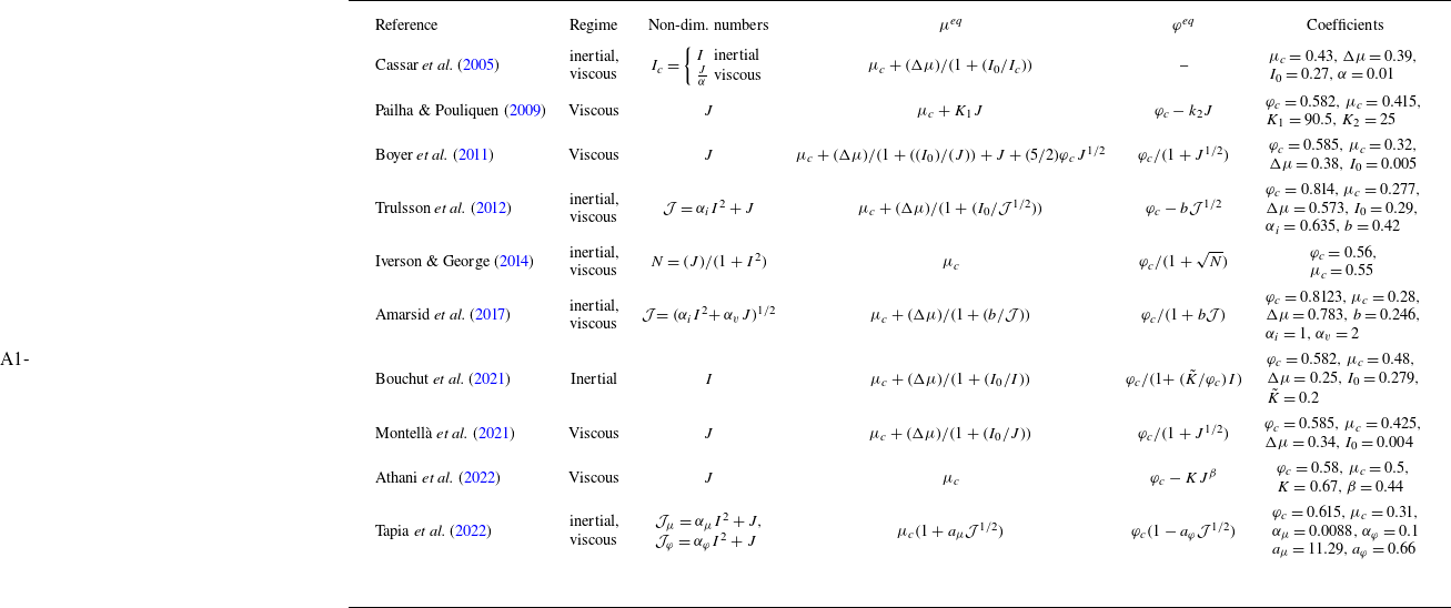
As in recent studies, constitutive laws describing steady uniform flows (i.e. at the critical state) are written in terms of a combination of two dimensionless numbers, based on the assumption of additivity of inertial and viscous stresses (Cassar, Nicolas & Pouliquen Reference Cassar, Nicolas and Pouliquen2005; Boyer, Guazzelli & Pouliquen Reference Boyer, Guazzelli and Pouliquen2011; Trulsson, Andreotti & Claudin Reference Trulsson, Andreotti and Claudin2012; Amarsid et al. Reference Amarsid, Delenne, Mutabaruka, Monerie, Perales and Radjai2017; Tapia et al. Reference Tapia, Ichihara, Pouliquen and Guazzelli2022). These two independent numbers
 $I$
and
$I$
and
 $J$
characterise inertial and viscous regimes, respectively:
$J$
characterise inertial and viscous regimes, respectively:
 \begin{equation} I=\frac {d\,\dot \gamma }{\sqrt {{p_s}_{|b}/\rho _s}},\quad J=\frac {\eta _f \, \dot \gamma }{{p_s}_{|b}}, \end{equation}
where
 ${p_s}_{|b}$
represents the solid pressure at the bottom. At imposed pressure, the shear stress is proportional to
${p_s}_{|b}$
represents the solid pressure at the bottom. At imposed pressure, the shear stress is proportional to
 $I^2$
in the inertial regime and to
$I^2$
in the inertial regime and to
 $J$
in the viscous regime. The transition between these regimes is given by the Stokes number, defined by the ratio between the inertial and viscous stress scales (see Tapia et al. Reference Tapia, Ichihara, Pouliquen and Guazzelli2022)
$J$
in the viscous regime. The transition between these regimes is given by the Stokes number, defined by the ratio between the inertial and viscous stress scales (see Tapia et al. Reference Tapia, Ichihara, Pouliquen and Guazzelli2022)
 \begin{equation} { {St}}=I^2/J= \frac {\rho _s \dot \gamma d^2}{\eta _f}. \end{equation}
To describe all possible regimes from inertial to viscous flows, different combinations of
 $I$
and
$I$
and
 $J$
have been proposed in the literature (see table 2). These inertial–viscous numbers may all be written as
$J$
have been proposed in the literature (see table 2). These inertial–viscous numbers may all be written as
 \begin{equation} {\mathcal {J}}=\alpha _i I^2 + \alpha _v J, \end{equation}
where
 $\alpha _i$
and
$\alpha _i$
and
 $\alpha _v$
are two constant coefficients that define the relative importance of inertial and viscous numbers, and depend on the material involved. Tapia et al. (Reference Tapia, Ichihara, Pouliquen and Guazzelli2022) showed that
$\alpha _v$
are two constant coefficients that define the relative importance of inertial and viscous numbers, and depend on the material involved. Tapia et al. (Reference Tapia, Ichihara, Pouliquen and Guazzelli2022) showed that
 $\alpha _i$
and
$\alpha _i$
and
 $\alpha _v$
are not the same in the rheological laws defining
$\alpha _v$
are not the same in the rheological laws defining
 $\varphi ^{\textit{eq}}$
and
$\varphi ^{\textit{eq}}$
and
 $\mu ^{\textit{eq}}$
, respectively. Note that inertial–viscous numbers can also be written in terms of the Stokes number:
$\mu ^{\textit{eq}}$
, respectively. Note that inertial–viscous numbers can also be written in terms of the Stokes number:
 \begin{align} \mathcal {J}= I^2 \left (\alpha _i +\alpha _v \frac {1}{ {St}}\right )=J\left (\alpha _i\,{ {St}}+\alpha _v \right ). \end{align}
The inertial regime corresponds to large Stokes numbers and thus to
 $\mathcal {J}\simeq \alpha _i I^2$
, and the viscous regime to small Stokes numbers and thus to
$\mathcal {J}\simeq \alpha _i I^2$
, and the viscous regime to small Stokes numbers and thus to
 $\mathcal {J} \simeq \alpha _v J$
. We choose here a rheological law as done by Tapia et al. (Reference Tapia, Ichihara, Pouliquen and Guazzelli2022), even though we use nonlinear functions to define
$\mathcal {J} \simeq \alpha _v J$
. We choose here a rheological law as done by Tapia et al. (Reference Tapia, Ichihara, Pouliquen and Guazzelli2022), even though we use nonlinear functions to define
 $\varphi ^{\textit{eq}}$
and
$\varphi ^{\textit{eq}}$
and
 $\mu ^{\textit{eq}}$
, to bound their value for infinite
$\mu ^{\textit{eq}}$
, to bound their value for infinite
 $\mathcal {J}$
numbers. We define two inertial–viscous numbers involved in the critical-state solid volume fraction
$\mathcal {J}$
numbers. We define two inertial–viscous numbers involved in the critical-state solid volume fraction
 $\varphi ^{\textit{eq}}$
and friction coefficient
$\varphi ^{\textit{eq}}$
and friction coefficient
 $\mu ^{\textit{eq}}$
, respectively,
$\mu ^{\textit{eq}}$
, respectively,
 \begin{equation} \mathcal {J}_\varphi =\alpha _\varphi I^2+ J \quad \mbox {and} \quad \mathcal {J}_\mu =\alpha _\mu I^2+J, \end{equation}
where
 $\alpha _\varphi$
and
$\alpha _\varphi$
and
 $\alpha _\mu$
are two constant coefficients. The critical-state solid volume fraction is then defined as
$\alpha _\mu$
are two constant coefficients. The critical-state solid volume fraction is then defined as
 \begin{equation} \varphi ^{\textit{eq}}(\mathcal {J}_\varphi )=\frac {\varphi _c}{1+b_\varphi \mathcal {J}_\varphi ^{1/2}}, \end{equation}
where
 $b_\varphi$
is a calibration constant and
$b_\varphi$
is a calibration constant and
 $\varphi _c$
the static value of the critical-state solid volume fraction. Finally, the critical friction coefficient is defined as
$\varphi _c$
the static value of the critical-state solid volume fraction. Finally, the critical friction coefficient is defined as
 \begin{equation} \mu ^{\textit{eq}}(\mathcal {J}_\mu )=\mu _c +\frac {\Delta \mu }{1+\frac {I_0}{\mathcal {J}_\mu ^{1/2}}}, \end{equation}
where
 $\mu _c=\tan \delta$
is the static value of the critical-state friction coefficient, with
$\mu _c=\tan \delta$
is the static value of the critical-state friction coefficient, with
 $\delta$
the granular friction angle;
$\delta$
the granular friction angle;
 $\Delta \mu$
and
$\Delta \mu$
and
 $I_0$
are constant parameters (see table 2 for their values in the literature). Numerical simulations will be performed in § 5 to show how strongly these coefficients impact the flow behaviour.
$I_0$
are constant parameters (see table 2 for their values in the literature). Numerical simulations will be performed in § 5 to show how strongly these coefficients impact the flow behaviour.
Table 2. Rheological laws in the literature.
2.2.2. Dilatancy law
Following Roux & Radjai (Reference Roux and Radjai1998); Pailha et al. (Reference Pailha, Nicolas and Pouliquen2008), the dilatancy law is given by
 \begin{equation} \textrm {div}\, \boldsymbol{V} =\Phi ={\dot \gamma }\tan \psi, \end{equation}
with
 $\psi$
the dilatancy angle related to the deviation from critical state, defined by
$\psi$
the dilatancy angle related to the deviation from critical state, defined by
 \begin{equation} \tan \psi = K \left (\varphi -\varphi ^{\textit{eq}}(\mathcal {J}_\varphi )\right ), \end{equation}
and the shear rate approximated by
 \begin{equation} \dot \gamma =\frac 52 \frac {|\boldsymbol{V}|}{h_m}. \end{equation}
Note that this value is obtained by Cassar et al. (Reference Cassar, Nicolas and Pouliquen2005) for the inertial regime of submarine granular flows described by the
 $\mu (I)$
-rheology. In our case, the equivalent calculation for our
$\mu (I)$
-rheology. In our case, the equivalent calculation for our
 $\mu (\mathcal {J}_\mu )$
-rheology also gives a Bagnold-like profile, namely,
$\mu (\mathcal {J}_\mu )$
-rheology also gives a Bagnold-like profile, namely,
 \begin{align} \boldsymbol{V}(z) = \frac {1}{2\alpha _\mu d^2 \rho _s}\left (-\eta _f z - \frac {2}{3A}\left ((\eta _f^2+A(h_m-z))^{3/2}-(\eta _f^2+Ah_m)^{3/2}\right )\right ), \end{align}
where
 $A=4\alpha _\mu d^2 \rho _s \varphi _c(\rho _s-\rho _f) g\cos \theta \mathcal {J}_\mu$
. The approximated value of
$A=4\alpha _\mu d^2 \rho _s \varphi _c(\rho _s-\rho _f) g\cos \theta \mathcal {J}_\mu$
. The approximated value of
 $\dot \gamma$
is then calculated from the related averaged velocity that leads to a fifth-order polynomial in
$\dot \gamma$
is then calculated from the related averaged velocity that leads to a fifth-order polynomial in
 $\mathcal {J}_\mu$
, not easy to solve. To find an approximation, we neglect terms in
$\mathcal {J}_\mu$
, not easy to solve. To find an approximation, we neglect terms in
 $\eta _f^2$
and we find that
$\eta _f^2$
and we find that
 $\dot \gamma \sim 2.517({|\boldsymbol{V}|}/{h_m})$
. As a result, the coefficient
$\dot \gamma \sim 2.517({|\boldsymbol{V}|}/{h_m})$
. As a result, the coefficient
 $5/2$
also gives a good approximation of
$5/2$
also gives a good approximation of
 $\dot \gamma$
for the
$\dot \gamma$
for the
 $\mu (\mathcal {J}_\mu )$
-rheology. The limit
$\mu (\mathcal {J}_\mu )$
-rheology. The limit
 $\alpha _\mu \to 0$
reduces the number
$\alpha _\mu \to 0$
reduces the number
 $\mathcal {J}_\mu$
to the pure viscous number
$\mathcal {J}_\mu$
to the pure viscous number
 $J$
. In (2.14) for
$J$
. In (2.14) for
 $\boldsymbol{V}(z)$
, this limit gives indeed the purely viscous parabolic profile as in (12) of Cassar et al. (Reference Cassar, Nicolas and Pouliquen2005),
$\boldsymbol{V}(z)$
, this limit gives indeed the purely viscous parabolic profile as in (12) of Cassar et al. (Reference Cassar, Nicolas and Pouliquen2005),
 $ \boldsymbol{V}(z)= ( 1/2) ({J}/{\eta _f})\varphi _c(\rho _s-\rho _f) g\cos \theta ( h_m^2 - (h_m-z)^2 ).$
When the flow is denser than the flow in the critical state (
 $\varphi \gt \varphi ^{\textit{eq}}$
), the dilatancy angle
$\varphi \gt \varphi ^{\textit{eq}}$
), the dilatancy angle
 $\psi$
is positive and the solid phase dilates, and vice versa. The friction coefficient in the transient regime involves the dilatancy angle as
$\psi$
is positive and the solid phase dilates, and vice versa. The friction coefficient in the transient regime involves the dilatancy angle as
 \begin{equation} \mu =\left (\mu ^{\textit{eq}}(\mathcal {J}_\mu )+\tan \psi \right )_+. \end{equation}
Note that the dilatancy rules (2.11), (2.15) for
 $\varphi$
and
$\varphi$
and
 $\mu$
use the most simple linear expansions involving the dilatancy factor (2.12) expressed linearly in terms of the deviation from critical state. A positive part has been put in (2.15) as a minimal correction to ensure that
$\mu$
use the most simple linear expansions involving the dilatancy factor (2.12) expressed linearly in terms of the deviation from critical state. A positive part has been put in (2.15) as a minimal correction to ensure that
 $\mu$
is non-negative.
$\mu$
is non-negative.
Remark 1. The
 $\mu (I)$
-rheology is ill-posed in the incompressible regime (Barker et al. 2015), but it is well-posed in the compressible regime (Schaeffer et al. Reference Schaeffer, Barker, Tsuji, Gremaud, Shearer and Gray2019; Barker et al. 2023). According to these two papers, the compressible regime is characterised by a dilatancy law and a friction law as we have in (2.11) and (2.15). The context is thus suitable for ensuring well-posedness, though stability conditions must be analysed further. However, this is beyond the scope of this article. Depth-averaged models are generally hyperbolic under reasonable conditions, such as limited velocity differences for models with several unknown velocities. Viscous terms, as noted by Baker (2016), can eventually relax this condition. Hyperbolicity implies well-posedness as long as source terms do not contain derivatives of unknowns (question mark). This is the case here since
$\mu (I)$
-rheology is ill-posed in the incompressible regime (Barker et al. 2015), but it is well-posed in the compressible regime (Schaeffer et al. Reference Schaeffer, Barker, Tsuji, Gremaud, Shearer and Gray2019; Barker et al. 2023). According to these two papers, the compressible regime is characterised by a dilatancy law and a friction law as we have in (2.11) and (2.15). The context is thus suitable for ensuring well-posedness, though stability conditions must be analysed further. However, this is beyond the scope of this article. Depth-averaged models are generally hyperbolic under reasonable conditions, such as limited velocity differences for models with several unknown velocities. Viscous terms, as noted by Baker (2016), can eventually relax this condition. Hyperbolicity implies well-posedness as long as source terms do not contain derivatives of unknowns (question mark). This is the case here since
 $\dot \gamma$
is approximated by (2.13) that avoids any derivative, and this is a main difference with non-averaged models.
$\dot \gamma$
is approximated by (2.13) that avoids any derivative, and this is a main difference with non-averaged models.
2.3. Two-layer model with three velocities (model A1)
Let us present here the full model derived by Bouchut et al. (Reference Bouchut, Fernández-Nieto, Mangeney and Narbona-Reina2016) with the rheology defined above. This model describes the behaviour of a mixture with different velocities for the solid and fluid phases
 $\boldsymbol{u}$
,
$\boldsymbol{u}$
,
 $\boldsymbol{v}$
, respectively, as well as an upper fluid layer of velocity
$\boldsymbol{v}$
, respectively, as well as an upper fluid layer of velocity
 $\boldsymbol{u}_f$
(see figure 1). Only slight modifications have been made in the model derivation compared with Bouchut et al. (Reference Bouchut, Fernández-Nieto, Mangeney and Narbona-Reina2016), owing to the different choice of conditions at the bottom and at the mixture/upper fluid interface, as well as to the description of viscous dissipation for the fluid phase (see supplementary material, §§ S.A.2 and S.A.3, for details). The free surface, interfacial and basal boundary conditions are summarised in the supplementary material, § S.A.1.
$\boldsymbol{u}_f$
(see figure 1). Only slight modifications have been made in the model derivation compared with Bouchut et al. (Reference Bouchut, Fernández-Nieto, Mangeney and Narbona-Reina2016), owing to the different choice of conditions at the bottom and at the mixture/upper fluid interface, as well as to the description of viscous dissipation for the fluid phase (see supplementary material, §§ S.A.2 and S.A.3, for details). The free surface, interfacial and basal boundary conditions are summarised in the supplementary material, § S.A.1.
2.3.1. Conservation equations and closure relations
The mass conservation equations for the solid and fluid phases in the mixture and for the fluid phase in the upper-layer read, respectively,
 \begin{equation} \partial _t(\rho _s\varphi h_m)+\nabla \cdot (\rho _s\varphi h_m\boldsymbol{v})=0, \end{equation}
 \begin{equation} \partial _t\bigl (\rho _f(1-\varphi )h_m\bigr )+\nabla \cdot \bigl (\rho _f(1-\varphi )h_m\boldsymbol{u}\bigr )=-\rho _f\mathcal {V}_f, \end{equation}
 \begin{equation} \partial _t (\rho _f h_f)+\nabla \cdot (\rho _fh_f\boldsymbol{u}_f)=\rho _f\mathcal {V}_f. \end{equation}
The corresponding momentum conservation equations are
 \begin{equation} \partial _t(\rho _s\varphi h_m \boldsymbol{v})+\nabla \cdot (\rho _s\varphi h_m\boldsymbol{v}\otimes \boldsymbol{v})=S_v, \end{equation}
 \begin{equation} \partial _t (\rho _f(1-\varphi ) h_m \boldsymbol{u}) +\nabla \cdot (\rho _f(1-\varphi )h_m\boldsymbol{u}\otimes \boldsymbol{u}) = S_u, \end{equation}
 \begin{equation} \partial _t (\rho _f h_f\boldsymbol{u}_f)+\nabla \cdot (\rho _f h_f \boldsymbol{u}_f\otimes \boldsymbol{u}_f) = S_f. \end{equation}
The source terms are given, respectively, by
 \begin{align} S_v&= \underbrace {-g\cos \theta \varphi h_m \big (\rho _s\nabla (b+h_m)+\rho _f \nabla h_f\big ) -g\cos \theta (\rho _s-\rho _f)\frac {h_m^2}{2} \nabla \varphi }_{\mbox {hydrostatic pressure}}\nonumber\\&\quad +\underbrace {(1-\varphi ) h_m \overline {{\nabla p^e_{f_m}}}}_{\mbox {excess pore pressure}} +\underbrace {\beta h_m (\boldsymbol{u}-\boldsymbol{v})}_{\mbox {drag in mixture}} +\underbrace {{k_f}\frac {\rho _s \varphi }{\rho }(\boldsymbol{u}_f-\boldsymbol{v}_m)}_{\mbox {drag with upper-fluid}} \nonumber \\ &\quad -\underbrace {\mu \,\mathop {\textrm {sgn}}(\boldsymbol{v})\left (\varphi (\rho _s-\rho _f)g\cos \theta h_m-(p^e_{f_m})_{|b}\right )}_{\mbox {solid bottom friction}} -\underbrace {\varphi h_m \rho _s g\textrm {sin} {\theta \boldsymbol e}_x}_{\mbox {gravity}}, \end{align}
 \begin{align} S_u = -\underbrace {(1-\varphi ) h_m \rho _f g\cos \theta \nabla (b+h_m+h_f)}_{\mbox {hydrostatic pressure}} -\underbrace {(1-\varphi ) h_m \overline {{\nabla p^e_{f_m}}}}_{\mbox {excess pore pressure}} \nonumber \\ \quad -\underbrace {((1-\lambda _f)\boldsymbol{u}+\lambda _f \boldsymbol{u}_f)\rho _f\mathcal {V}_f }_{\mbox {fluid transfer}} -\underbrace {\beta h_m (\boldsymbol{u}-\boldsymbol{v})}_{\mbox {drag in mixture}} +\underbrace {k_f \frac {\rho _f (1-\varphi )}{\rho } (\boldsymbol{u}_f-\boldsymbol{v}_m)}_{\mbox {drag with upper-fluid}} \nonumber \\ \quad -\underbrace {\frac 52\frac {\eta _e(1-\varphi )}{h_m}\boldsymbol{u} }_{\mbox {fluid bottom friction}} -\underbrace {(1-\varphi ) h_m \rho _f g \textrm {sin} \theta {\boldsymbol e}_x}_{\mbox {gravity}}, \end{align}
 \begin{align} S_f &= -\underbrace {\rho _f h_f g\cos \theta \nabla (b+h_m+h_f)}_{\mbox {hydrostatic pressure}} +\underbrace {((1-\lambda _f)\boldsymbol{u}+\lambda _f \boldsymbol{u}_f)\rho _f\mathcal {V}_f}_{\mbox {fluid transfer}} \nonumber \\ & \quad -\underbrace {k_f(\boldsymbol{u}_f-\boldsymbol{v}_m)}_{\mbox {drag with upper-fluid}} -\underbrace {\rho _f h_f g\textrm {sin} \theta {\boldsymbol e}_x}_{\mbox {gravity}}, \end{align}
where the coefficient
 $k_f$
and the effective viscosity
$k_f$
and the effective viscosity
 $\eta _e$
are
$\eta _e$
are
 \begin{equation} k_f= m_f \frac {\rho h_m\rho _f h_f}{\rho h_m+\rho _f h_f} |\boldsymbol{u}_f-\boldsymbol{v}_m|\qquad \mbox {and} \qquad \eta _e=\eta _f \left (1+\frac 52 \varphi \right ), \end{equation}
with
 $m_f$
a constant coefficient (Poulain et al. Reference Poulain2022). (The effective shear viscosity
$m_f$
a constant coefficient (Poulain et al. Reference Poulain2022). (The effective shear viscosity
 $\eta _e$
is approximated using Einstein’s formula (Einstein Reference Einstein1906) to take into account the presence of granular material (see for example (Chauchat & Médale Reference Chauchat and Médale2010; Boyer et al. Reference Boyer, Guazzelli and Pouliquen2011; Baumgarten & Kamrin Reference Baumgarten and Kamrin2019)), see also supplementary material, § S.A.2.) The excess pore pressure
$\eta _e$
is approximated using Einstein’s formula (Einstein Reference Einstein1906) to take into account the presence of granular material (see for example (Chauchat & Médale Reference Chauchat and Médale2010; Boyer et al. Reference Boyer, Guazzelli and Pouliquen2011; Baumgarten & Kamrin Reference Baumgarten and Kamrin2019)), see also supplementary material, § S.A.2.) The excess pore pressure
 $p^e_{f_m}$
appears in the depth-averaged value of
$p^e_{f_m}$
appears in the depth-averaged value of
 $\nabla p^e_{f_m}$
:
$\nabla p^e_{f_m}$
:
 \begin{equation} \overline {{\nabla p^e_{f_m}}}=\frac {1}{h_m}\Big ( \nabla (h_m \overline {p^e_{f_m}})+({p^e_{f_m}})_{|b}\nabla b\Big ), \end{equation}
with
 $p^e_{f_m}$
at the bottom and the depth-averaged value of
$p^e_{f_m}$
at the bottom and the depth-averaged value of
 $p^e_{f_m}$
given by
$p^e_{f_m}$
given by
 \begin{equation} (p^e_{f_m})_{|b}=-\frac {\beta }{(1-\varphi )^2}\frac {h_m^2}{2}\Phi, \quad \overline {p^e_{f_m}}=-\frac {\beta }{(1-\varphi )^2}\frac {h_m^2}{3}\Phi, \end{equation}
with the drag coefficient
 $\beta$
defined by Pailha & Pouliquen (Reference Pailha and Pouliquen2009),
$\beta$
defined by Pailha & Pouliquen (Reference Pailha and Pouliquen2009),
 \begin{equation} \beta = (1-\varphi )^2\frac {\eta _f}{k}\quad \textrm {with} \quad k=\frac {(1-\varphi )^3d^2}{150 \varphi ^2}, \end{equation}
where
 $d$
is the grain diameter,
$d$
is the grain diameter,
 $\eta _f$
the dynamic viscosity of the fluid and
$\eta _f$
the dynamic viscosity of the fluid and
 $k$
the hydraulic permeability of the granular aggregate. Similar parameters are used by Baumgarten & Kamrin (Reference Baumgarten and Kamrin2019) (see supplementary material, § S.A.4.3). The dilatancy function is defined by
$k$
the hydraulic permeability of the granular aggregate. Similar parameters are used by Baumgarten & Kamrin (Reference Baumgarten and Kamrin2019) (see supplementary material, § S.A.4.3). The dilatancy function is defined by
 \begin{equation} \Phi =K\dot \gamma (\varphi -\varphi ^{\textit{eq}}), \end{equation}
and the rheological laws give
 \begin{align*} \varphi ^{\textit{eq}}=\dfrac {\varphi _c}{1+b_\varphi \mathcal {J}_\varphi ^{1/2}}\quad \textrm {with} \quad \mathcal {J}_\varphi =\alpha _\varphi I^2+J,\\ \mu ^{\textit{eq}}=\mu _c +\dfrac {\Delta \mu }{1+I_0/\mathcal {J}_\mu ^{1/2}}\quad \textrm {with} \quad \mathcal {J}_\mu =\alpha _\mu I^2+J,\end{align*}
where
 \begin{align} I=\dfrac {d\,\dot \gamma }{\sqrt {{p_s}_{|b}/\rho _s}},\quad J=\dfrac {\eta _f \dot \gamma }{{p_s}_{|b}},\quad \dot \gamma =\dfrac 52 \dfrac {|\boldsymbol{v}|}{h_m} \quad {p_s}_{|b}=\varphi (\rho _s-\rho _f)g\cos \theta h_m-(p^e_{f_m})_{|b}. \end{align}
Owing to dilatancy, the friction coefficient is defined as
 \begin{equation} \mu =\left (\mu ^{\textit{eq}}+K(\varphi -\varphi ^{\textit{eq}})\right )_+. \end{equation}
The fluid transfer rate reads
 \begin{equation} \mathcal {V}_f=-h_m \Phi -\nabla \cdot \big (h_m(1-\varphi )(\boldsymbol{u}-\boldsymbol{v})\big ). \end{equation}
The transfer of fluid momentum between the mixture and the upper fluid layer ends up in the term
 $((1-\lambda _f) \boldsymbol{u} + \lambda _f \boldsymbol{u}_f)\rho _f \mathcal {V}_f$
in the fluid momentum equations (2.18b
), (2.18c
), where
$((1-\lambda _f) \boldsymbol{u} + \lambda _f \boldsymbol{u}_f)\rho _f \mathcal {V}_f$
in the fluid momentum equations (2.18b
), (2.18c
), where
 $\lambda _f$
is a parameter describing the stress distribution between the fluid and solid phases at the interface between the layers (see supplementary material, § S.A.3, for details). We define two possible choices for this arbitrary parameter:
$\lambda _f$
is a parameter describing the stress distribution between the fluid and solid phases at the interface between the layers (see supplementary material, § S.A.3, for details). We define two possible choices for this arbitrary parameter:
 \begin{equation} \lambda _f=\frac 12 -\frac 12 \mathop {\textrm {sgn}}(\mathcal {V}_f) \delta _f,\quad \delta _f=\left \{ \begin{array}{l} 0\quad \textrm {centered distribution,}\\ 1 \quad \textrm {upwind distribution.}\end{array}\right . \end{equation}
As a result, if we choose
 $\delta _f=0$
, the fluid velocity at the interface defined by
$\delta _f=0$
, the fluid velocity at the interface defined by
 $(1-\lambda _f) \boldsymbol{u} + \lambda _f \boldsymbol{u}_f$
reduces to
$(1-\lambda _f) \boldsymbol{u} + \lambda _f \boldsymbol{u}_f$
reduces to
 $(\boldsymbol{u}+\boldsymbol{u}_f)/2$
, while if we choose
$(\boldsymbol{u}+\boldsymbol{u}_f)/2$
, while if we choose
 $\delta _f=1$
, this velocity depends on the sign of
$\delta _f=1$
, this velocity depends on the sign of
 $\mathcal {V}_f$
. In this case, if the fluid is expelled from the mixture,
$\mathcal {V}_f$
. In this case, if the fluid is expelled from the mixture,
 $\mathcal {V}_f\gt 0$
and
$\mathcal {V}_f\gt 0$
and
 $\lambda _f=0$
, so that the velocity is
$\lambda _f=0$
, so that the velocity is
 $\boldsymbol{u}$
. However, if the fluid is sucked into the mixture,
$\boldsymbol{u}$
. However, if the fluid is sucked into the mixture,
 $\mathcal {V}_f\lt 0$
and
$\mathcal {V}_f\lt 0$
and
 $\lambda _f=1$
, and the velocity is
$\lambda _f=1$
, and the velocity is
 $\boldsymbol{u}_f$
.
$\boldsymbol{u}_f$
.
Note that, as exposed by Bouchut et al. (Reference Bouchut, Fernández-Nieto, Mangeney and Narbona-Reina2016), the expression (2.25) of the fluid transfer rate
 $\mathcal {V}_f$
is obtained from the mass equations together with the transport of the solid volume fraction
$\mathcal {V}_f$
is obtained from the mass equations together with the transport of the solid volume fraction
 \begin{equation} \partial _t\varphi +\boldsymbol{v}\cdot \nabla \varphi =-\varphi \Phi \end{equation}
that constitutes an alternative scalar equation to be considered instead of (2.25).
2.3.2. Computation of the basal solid pressure
A first approach to compute the solid pressure at the bottom
 ${p_s}_{|b}$
appearing in the granular friction term is to combine the above relations that implicitly define
${p_s}_{|b}$
appearing in the granular friction term is to combine the above relations that implicitly define
 ${p_s}_{|b}$
. Indeed,
${p_s}_{|b}$
. Indeed,
 ${p_s}_{|b}$
depends on
${p_s}_{|b}$
depends on
 ${p^e_{f_m}}_{|b}$
(see (2.23)) that can be expressed as a function of
${p^e_{f_m}}_{|b}$
(see (2.23)) that can be expressed as a function of
 $\Phi$
(see (2.20b
)), that is a function of
$\Phi$
(see (2.20b
)), that is a function of
 $\varphi ^{\textit{eq}}$
(see (2.22)) that itself can be expressed as a function of
$\varphi ^{\textit{eq}}$
(see (2.22)) that itself can be expressed as a function of
 ${p_s}_{|b}$
(see (2.23)). Combining these expressions, we find that
${p_s}_{|b}$
(see (2.23)). Combining these expressions, we find that
 $\sqrt {{p_s}_{|b}}$
is the positive root of the third-order polynomial,
$\sqrt {{p_s}_{|b}}$
is the positive root of the third-order polynomial,
 \begin{equation} \begin{array}{l} \displaystyle (\sqrt {{p_s}_{|b}})^3 + A_2(\sqrt {{p_s}_{|b}})^2 \\ \displaystyle -(\varphi (\rho _s-\rho _f)g\cos \theta h_m + A_1(\varphi -\varphi _c)) (\sqrt {{p_s}_{|b}}) - A_2 (\varphi (\rho _s-\rho _f)g\cos \theta h_m + \varphi A_1)=0, \end{array} \end{equation}
with coefficients
 $ A_1= ({\beta }/{(1-\varphi )^2}) ({h_m^2}/{2})\dot \gamma K,\ A_2=b_\varphi \,(\alpha _\varphi d^2 \dot \gamma ^2 \rho _s + \eta _f \dot \gamma )^{1/2}$
. It can be shown that this equation has a unique positive root
$ A_1= ({\beta }/{(1-\varphi )^2}) ({h_m^2}/{2})\dot \gamma K,\ A_2=b_\varphi \,(\alpha _\varphi d^2 \dot \gamma ^2 \rho _s + \eta _f \dot \gamma )^{1/2}$
. It can be shown that this equation has a unique positive root
 ${p_s}_{|b}\gt 0$
. Note that the polynomial and therefore its root are not the same when changing the rheological laws. Even if solving this equation is simple in depth-averaged models, it becomes problematic when solving multilayer models with dilatancy (Garres-Díaz et al. Reference Garres-Díaz, Bouchut, Fernández-Nieto, Mangeney and Narbona-Reina2020). An alternative approach is to solve an evolution equation for the solid pressure as done by Iverson & George (Reference Iverson and George2014) instead of specifying the 3-D dilatancy closure
${p_s}_{|b}\gt 0$
. Note that the polynomial and therefore its root are not the same when changing the rheological laws. Even if solving this equation is simple in depth-averaged models, it becomes problematic when solving multilayer models with dilatancy (Garres-Díaz et al. Reference Garres-Díaz, Bouchut, Fernández-Nieto, Mangeney and Narbona-Reina2020). An alternative approach is to solve an evolution equation for the solid pressure as done by Iverson & George (Reference Iverson and George2014) instead of specifying the 3-D dilatancy closure
 $\Phi =\dot \gamma \tan \psi$
(see (2.11)). This equation may be deduced from the 3-D solid stress tensor equation proposed by Baumgarten & Kamrin (Reference Baumgarten and Kamrin2019), where a thermodynamic analysis of a two-phase mixture for elastic–plastic granular solid in a viscous fluid is performed to close the Jackson system. Under certain assumptions, mainly neglecting pure plastic behaviour (see supplementary material, § S.A.6, for details), we find the following equation for the solid pressure
$\Phi =\dot \gamma \tan \psi$
(see (2.11)). This equation may be deduced from the 3-D solid stress tensor equation proposed by Baumgarten & Kamrin (Reference Baumgarten and Kamrin2019), where a thermodynamic analysis of a two-phase mixture for elastic–plastic granular solid in a viscous fluid is performed to close the Jackson system. Under certain assumptions, mainly neglecting pure plastic behaviour (see supplementary material, § S.A.6, for details), we find the following equation for the solid pressure
 $p_s$
:
$p_s$
:
 \begin{equation} \frac 1B\Big (\partial _t p_s+ {\boldsymbol V}\cdot \nabla p_s\Big ) =- \nabla \cdot {\boldsymbol V}+\dot \gamma \tan \psi, \end{equation}
where
 $B= {E}/({3(1-2\nu )})$
is the elastic bulk modulus of the solid (here, the grains), and
$B= {E}/({3(1-2\nu )})$
is the elastic bulk modulus of the solid (here, the grains), and
 $E$
and
$E$
and
 $\nu$
are the Young modulus and the Poisson ratio, respectively. Typical values for glass beads are
$\nu$
are the Young modulus and the Poisson ratio, respectively. Typical values for glass beads are
 $E=70\times 10^9$
Pa and
$E=70\times 10^9$
Pa and
 $\nu =0.2$
, corresponding to a solid bulk modulus
$\nu =0.2$
, corresponding to a solid bulk modulus
 $B=38.9\times 10^9$
Pa, and for sand are
$B=38.9\times 10^9$
Pa, and for sand are
 $E=100\times 10^6$
Pa and
$E=100\times 10^6$
Pa and
 $\nu =0.4$
, corresponding to a solid bulk modulus
$\nu =0.4$
, corresponding to a solid bulk modulus
 $B=16.6\times 10^7$
Pa (Holtzman, Silin & Patzek Reference Holtzman, Silin and Patzek2009; Montellà et al. Reference Montellà, Chauchat, Bonamy, Weij, Keetels and Hsu2023). Note that (2.29) reduces to the 3-D dilatancy closure
$B=16.6\times 10^7$
Pa (Holtzman, Silin & Patzek Reference Holtzman, Silin and Patzek2009; Montellà et al. Reference Montellà, Chauchat, Bonamy, Weij, Keetels and Hsu2023). Note that (2.29) reduces to the 3-D dilatancy closure
 $\Phi =\dot \gamma \tan \psi$
when
$\Phi =\dot \gamma \tan \psi$
when
 $B$
tends to infinity. Using classical asymptotic assumptions and the depth-averaging process detailed in the supplementary material, § S.A.6, we obtain the following equation for the solid pressure at the bottom
$B$
tends to infinity. Using classical asymptotic assumptions and the depth-averaging process detailed in the supplementary material, § S.A.6, we obtain the following equation for the solid pressure at the bottom
 ${p_s}_{|b}$
:
${p_s}_{|b}$
:
 \begin{equation} \partial _t {p_s}_{|b}+\boldsymbol{v}\cdot \nabla {p_s}_{|b}=\tfrac {1}{4}(\rho _s-\rho _f)g\cos \theta \varphi h_m\nabla \cdot \boldsymbol{v}-\tfrac 32 B (\Phi -{\dot \gamma }\tan \psi ). \end{equation}
We still need to define
 $\Phi$
, which can be easily obtained by using the expression of the excess pore pressure in (2.20b) and
$\Phi$
, which can be easily obtained by using the expression of the excess pore pressure in (2.20b) and
 ${p_s}_{|b}$
in (2.23) as follows:
${p_s}_{|b}$
in (2.23) as follows:
 \begin{align} \Phi =-\frac {2(1-\varphi )^2}{\beta h_m^2} (p^e_{f_m})_{|b}, \quad \mbox {with}\quad (p^e_{f_m})_{|b}=-\Big ({p_s}_{|b}-h_m\varphi (\rho _s-\rho _f)g\cos \theta \Big ). \end{align}
See § S.A.6.1 of the supplementary material for a numerical comparison of these two approaches.
2.4. Origin and impact of dilatancy in mixture models
How dilatancy is accounted for in depth-averaged mixture models is somewhat hidden since it involves a motion in the
 $z$
-direction perpendicular to the slope, which is assumed to be small in these shallow models. The dilatancy law
$z$
-direction perpendicular to the slope, which is assumed to be small in these shallow models. The dilatancy law
 $\Phi$
clearly appears in the mass equations describing mass exchange in the systems (2.16), (2.27), taking into account (2.25).
$\Phi$
clearly appears in the mass equations describing mass exchange in the systems (2.16), (2.27), taking into account (2.25).
2.4.1. Dilatancy and pore fluid pressure
Dilatancy is also present in the momentum equation through the excess pore pressure at the bottom
 $(p^e_{f_m})_{|b}$
(see (2.20b
)), which represents the non-hydrostatic part of the pore fluid pressure
$(p^e_{f_m})_{|b}$
(see (2.20b
)), which represents the non-hydrostatic part of the pore fluid pressure
 $p_{f_m}$
in our model. It is very sensitive to contraction/dilation of the granular phase and impacts in turn the rheology of the fluidised granular material. Indeed,
$p_{f_m}$
in our model. It is very sensitive to contraction/dilation of the granular phase and impacts in turn the rheology of the fluidised granular material. Indeed,
 $(p^e_{f_m})_{|b}$
appears in the solid pressure at the bottom
$(p^e_{f_m})_{|b}$
appears in the solid pressure at the bottom
 ${p_s}_{|b}$
together with a hydrostatic term including buoyancy,
${p_s}_{|b}$
together with a hydrostatic term including buoyancy,
 \begin{equation} {p_s}_{|b}=\varphi (\rho _s-\rho _f)g\cos \theta h_m-(p^e_{f_m})_{|b}, \end{equation}
 ${p_s}_{|b}$
being directly involved in the friction law on the right-hand side of (2.18a
). The excess pore pressure
${p_s}_{|b}$
being directly involved in the friction law on the right-hand side of (2.18a
). The excess pore pressure
 $p^e_{f_m}$
is generated by the normal displacement produced by the dilation–contraction of the granular material saturated by the fluid and is originally defined as
$p^e_{f_m}$
is generated by the normal displacement produced by the dilation–contraction of the granular material saturated by the fluid and is originally defined as
 \begin{equation} p^e_{f_m}= \frac {\beta }{1-\varphi } \int _z^{b+h_m} (u^z-v^z) (z') {\textrm d}z', \end{equation}
where
 $u^z$
and
$u^z$
and
 $v^z$
represent the fluid and solid velocities respectively, in the direction normal to the inclined reference plane (see figure 1). (See (3.45) of Bouchut et al. (Reference Bouchut, Fernández-Nieto, Mangeney and Narbona-Reina2016) and § 3.5 in that paper for more details.) It appears as a non-hydrostatic contribution in the solid and fluid pressures in the mixture (see § 3.4 of Bouchut et al. (Reference Bouchut, Fernández-Nieto, Mangeney and Narbona-Reina2016) for details). From this definition, we see that the excess pore pressure is negative if the granular material goes up with respect to the fluid (
$v^z$
represent the fluid and solid velocities respectively, in the direction normal to the inclined reference plane (see figure 1). (See (3.45) of Bouchut et al. (Reference Bouchut, Fernández-Nieto, Mangeney and Narbona-Reina2016) and § 3.5 in that paper for more details.) It appears as a non-hydrostatic contribution in the solid and fluid pressures in the mixture (see § 3.4 of Bouchut et al. (Reference Bouchut, Fernández-Nieto, Mangeney and Narbona-Reina2016) for details). From this definition, we see that the excess pore pressure is negative if the granular material goes up with respect to the fluid (
 $v^z\gt u^z$
) in the case of dilation (
$v^z\gt u^z$
) in the case of dilation (
 $\Phi \gt 0$
), and is positive (
$\Phi \gt 0$
), and is positive (
 $v^z\lt u^z$
) in the opposite case of contraction (
$v^z\lt u^z$
) in the opposite case of contraction (
 $\Phi \lt 0$
). As only downslope velocities are considered in our shallow depth-averaged model, we replace the normal velocities (
$\Phi \lt 0$
). As only downslope velocities are considered in our shallow depth-averaged model, we replace the normal velocities (
 $u^z$
,
$u^z$
,
 $v^z$
) by the downslope velocities (
$v^z$
) by the downslope velocities (
 $u, v$
) using the dilatancy closure equation
$u, v$
) using the dilatancy closure equation
 $\textrm {div}\, \boldsymbol{V} =\Phi$
, leading to
$\textrm {div}\, \boldsymbol{V} =\Phi$
, leading to
 \begin{align} u^z-v^z =-\frac {z-b}{1-\varphi }\left (\Phi +\nabla \cdot ((1-\varphi )(\boldsymbol{u}-\boldsymbol{v}))\right) +(\boldsymbol{u}-\boldsymbol{v})\cdot \nabla b+\textit {O}(\epsilon ^3), \end{align}
with
 $\epsilon$
the ratio between the characteristic thickness and downslope extension of the flow, which is assumed to be small in shallow models. The pore pressure at the bottom thus becomes
$\epsilon$
the ratio between the characteristic thickness and downslope extension of the flow, which is assumed to be small in shallow models. The pore pressure at the bottom thus becomes
 \begin{align} \left(p^e_{f_m}\right)_{|b}&=\frac {\beta }{1-\varphi }\left ( -\frac 12\frac {h_m^2}{1-\varphi } \Phi -\frac 12\frac {h_m^2}{1-\varphi }\nabla \cdot ((1-\varphi )(\boldsymbol{u}-\boldsymbol{v}))\nonumber\right. \\&\quad\left. +\,h_m (\boldsymbol{u} -\boldsymbol{v})\cdot \nabla b+\textit {O}(\epsilon ^4) \right ). \end{align}
As proposed by Bouchut et al. (Reference Bouchut, Fernández-Nieto, Mangeney and Narbona-Reina2016), a high drag coefficient,
 $\beta \sim \epsilon ^{-1}$
, implies a small velocity difference,
$\beta \sim \epsilon ^{-1}$
, implies a small velocity difference,
 $\boldsymbol{u}-\boldsymbol{v}\sim \epsilon$
, so that, at order
$\boldsymbol{u}-\boldsymbol{v}\sim \epsilon$
, so that, at order
 $\epsilon ^2$
, we obtain the values of
$\epsilon ^2$
, we obtain the values of
 $(p^e_{f_m})_{|b}$
and
$(p^e_{f_m})_{|b}$
and
 $\overline {p^e_{f_m}}$
used in our model (2.20b). Using (2.22), the excess pore fluid pressure at the bottom thus reads
$\overline {p^e_{f_m}}$
used in our model (2.20b). Using (2.22), the excess pore fluid pressure at the bottom thus reads
 \begin{equation} (p^e_{f_m})_{|b}=-75\frac {\eta _f}{d^2}\frac {\varphi ^2}{(1-\varphi )^3}\left ( \varphi -\varphi ^{\textit{eq}} \right ) K \frac {5}{2} h_m|\boldsymbol{v}|. \end{equation}
As a result, the excess pore fluid pressure at the bottom directly depends on the deviation from the critical state (
 $\varphi -\varphi ^{\textit{eq}}$
) and, in particular, on its sign. If
$\varphi -\varphi ^{\textit{eq}}$
) and, in particular, on its sign. If
 $\varphi \gt \varphi ^{\textit{eq}}$
, the granular phase dilates and the excess pore pressure is negative and vice versa. In particular, the excess pore pressure is equal to zero in steady flows where
$\varphi \gt \varphi ^{\textit{eq}}$
, the granular phase dilates and the excess pore pressure is negative and vice versa. In particular, the excess pore pressure is equal to zero in steady flows where
 $\varphi =\varphi ^{\textit{eq}}$
, i.e. in the critical state. The absolute value of the excess pore fluid pressure increases as the viscosity of the fluid and the downslope solid flux increase and it decreases with increasing grain diameter as a result of higher permeability. To illustrate this, figure S13 (supplementary material) shows
$\varphi =\varphi ^{\textit{eq}}$
, i.e. in the critical state. The absolute value of the excess pore fluid pressure increases as the viscosity of the fluid and the downslope solid flux increase and it decreases with increasing grain diameter as a result of higher permeability. To illustrate this, figure S13 (supplementary material) shows
 $(p^e_{f_m})_{|b}/( \varphi -\varphi ^{\textit{eq}})$
as a function of
$(p^e_{f_m})_{|b}/( \varphi -\varphi ^{\textit{eq}})$
as a function of
 $\varphi$
for values of the parameters taken from Bouchut et al. (Reference Bouchut, Fernández-Nieto, Mangeney and Narbona-Reina2016).
$\varphi$
for values of the parameters taken from Bouchut et al. (Reference Bouchut, Fernández-Nieto, Mangeney and Narbona-Reina2016).
2.4.2. Dilatancy and fluid transfer rate
Another key quantity in debris flow models with dilatancy is the fluid transfer rate
 $\mathcal {V}_f$
between the mixture and upper fluid layers. The fluid mass transfer appears in the mass conservation equation (2.16). When
$\mathcal {V}_f$
between the mixture and upper fluid layers. The fluid mass transfer appears in the mass conservation equation (2.16). When
 $\mathcal {V}_f \gt 0$
, the fluid is expelled from the mixture region towards the fluid-only layer as depicted in figure 1, and vice versa. This fluid transfer rate is directly related to the dilatancy of the granular phase by (2.25) that leads, owing to (2.11) and (2.12), to
$\mathcal {V}_f \gt 0$
, the fluid is expelled from the mixture region towards the fluid-only layer as depicted in figure 1, and vice versa. This fluid transfer rate is directly related to the dilatancy of the granular phase by (2.25) that leads, owing to (2.11) and (2.12), to
 \begin{equation} \mathcal {V}_f=-h_m\dot \gamma K\left ( \varphi -\varphi ^{\textit{eq}} \right ) -\nabla \cdot \big (h_m(1-\varphi )(\boldsymbol{u}-\boldsymbol{v})\big ). \end{equation}
When
 $\varphi \gt \varphi ^{\textit{eq}}$
, the granular phase dilates and the first term in the fluid transfer rate is negative, which means that the fluid is sucked from the upper fluid layer into the mixture (figure 1), and vice versa. Note that the second term in (2.37) shows that, in principle, the fluid can still be transferred from one layer to the other when
$\varphi \gt \varphi ^{\textit{eq}}$
, the granular phase dilates and the first term in the fluid transfer rate is negative, which means that the fluid is sucked from the upper fluid layer into the mixture (figure 1), and vice versa. Note that the second term in (2.37) shows that, in principle, the fluid can still be transferred from one layer to the other when
 $\varphi =\varphi ^{\textit{eq}}$
, as long as
$\varphi =\varphi ^{\textit{eq}}$
, as long as
 $\boldsymbol{u}-\boldsymbol{v}\not =0$
. However, this situation is hardly ever achieved since the time scale for
$\boldsymbol{u}-\boldsymbol{v}\not =0$
. However, this situation is hardly ever achieved since the time scale for
 $\boldsymbol{u}$
and
$\boldsymbol{u}$
and
 $\boldsymbol{v}$
to be equal due to drag is much shorter than the time scale to reach the critical state (see (Bouchut et al. Reference Bouchut, Fernández-Nieto, Mangeney and Narbona-Reina2016)).
$\boldsymbol{v}$
to be equal due to drag is much shorter than the time scale to reach the critical state (see (Bouchut et al. Reference Bouchut, Fernández-Nieto, Mangeney and Narbona-Reina2016)).

Figure 3. Model A1, flow configuration and notation for the full two-layer model with three velocities: the fluid and solid velocities in the mixture
 $\boldsymbol{u}$
and
$\boldsymbol{u}$
and
 $\boldsymbol{v}$
and the velocity of the upper fluid layer
$\boldsymbol{v}$
and the velocity of the upper fluid layer
 $\boldsymbol{u}_f$
(Bouchut et al. Reference Bouchut, Fernández-Nieto, Mangeney and Narbona-Reina2016). The derived simplified models are model A2, the same as model A1 except that the solid and fluid velocities in the mixture are assumed to be the same (
$\boldsymbol{u}_f$
(Bouchut et al. Reference Bouchut, Fernández-Nieto, Mangeney and Narbona-Reina2016). The derived simplified models are model A2, the same as model A1 except that the solid and fluid velocities in the mixture are assumed to be the same (
 $\boldsymbol{u}=\boldsymbol{v}$
); model B1, the same as model A1 except that the velocity of the upper fluid layer is assumed to be the mean velocity of the mixture (
$\boldsymbol{u}=\boldsymbol{v}$
); model B1, the same as model A1 except that the velocity of the upper fluid layer is assumed to be the mean velocity of the mixture (
 $\boldsymbol{u}_f=\boldsymbol{v}_m$
); model B2, the same as model A1 except that all the velocities are assumed to be the same (
$\boldsymbol{u}_f=\boldsymbol{v}_m$
); model B2, the same as model A1 except that all the velocities are assumed to be the same (
 $\boldsymbol{u}=\boldsymbol{v}=\boldsymbol{u}_f$
); model C1, a one-layer model with a virtual thickness
$\boldsymbol{u}=\boldsymbol{v}=\boldsymbol{u}_f$
); model C1, a one-layer model with a virtual thickness
 $H$
, a solid velocity
$H$
, a solid velocity
 $\boldsymbol{v}$
and a fluid velocity
$\boldsymbol{v}$
and a fluid velocity
 $\boldsymbol{u}$
; model C2, the same as model C1 but with identical velocities for the solid and fluid phases (
$\boldsymbol{u}$
; model C2, the same as model C1 but with identical velocities for the solid and fluid phases (
 $\boldsymbol{u}=\boldsymbol{v}$
).
$\boldsymbol{u}=\boldsymbol{v}$
).
2.4.3. Relation between the key variables
It is worth pointing out that the key variables describing the deviation to the critical state (compaction/dilation) in the model are all related to dilation angle
 $\tan \psi$
since
$\tan \psi$
since
 \begin{equation} \tan \psi =-(p^e_{f_m})_{|b} \frac {2(1-\varphi )^2}{\dot \gamma \beta h_m^2}=\mu - \mu ^{\textit{eq}}=K\left (\varphi -\varphi ^{\textit{eq}}\right )=\frac {\textrm {div}\, \mathbf {\boldsymbol V}}{\dot \gamma }. \end{equation}
3. Simplest one-velocity models
We are going to introduce several simplified models, sketched in figure 3. They are derived from the full two-layer and three-velocity model A1 described in § 2.3. We will present here only the two simplest models that involve only one velocity: (i) the two-layer model B2; (ii) the one-layer model with a virtual thickness (model C2). The two-layer model with a different velocity for the mixture and the upper fluid layer (model A2) was presented by Drach (Reference Drach2023) and is given in supplementary material, § S.C.2.2.
3.1. Two-layer model with one velocity (model B2)
3.1.1. System of equations
The procedure to obtain this simplified model is as follows. A key assumption is that we consider a high friction coefficient
 $\beta$
between the solid and fluid phases in the mixture, and a high friction coefficient
$\beta$
between the solid and fluid phases in the mixture, and a high friction coefficient
 $k_f$
between the layers. This results in a single downslope velocity for the whole system
$k_f$
between the layers. This results in a single downslope velocity for the whole system
 \begin{align} \boldsymbol{u}=\boldsymbol{v}=\boldsymbol{u}_f. \end{align}
We keep the notation
 $\boldsymbol{v}$
for the single velocity (figure 3
d). In this two-layer model, the system has four unknowns
$\boldsymbol{v}$
for the single velocity (figure 3
d). In this two-layer model, the system has four unknowns
 $h_m, h_f, \varphi \ \textrm {and}\ \boldsymbol{v}$
, and is described by the following equations (remember that
$h_m, h_f, \varphi \ \textrm {and}\ \boldsymbol{v}$
, and is described by the following equations (remember that
 $\rho =\rho _s\varphi + \rho _f (1-\varphi )$
): the total and upper fluid layer mass conservation equations
$\rho =\rho _s\varphi + \rho _f (1-\varphi )$
): the total and upper fluid layer mass conservation equations
 \begin{equation} \partial _t\big (\rho h_m+ \rho _f h_f\big )+\nabla \cdot \Big ( \big (\rho h_m+\rho _f h_f \big ) \boldsymbol{v} \Big )=0, \end{equation}
 \begin{equation} \partial _t (\rho _f h_f)+\nabla \cdot (\rho _f h_f \boldsymbol{v})=\rho _f \mathcal {V}_f, \end{equation}
the volume fraction equation
 \begin{equation} \partial _t\varphi +\boldsymbol{v}\cdot \nabla \varphi =-\varphi \Phi, \end{equation}
and the total momentum conservation equation
 \begin{align} &\partial _t\bigl ((\rho h_m+ \rho _f h_f) v\bigr )+{\nabla} \cdot ((\rho h_m+ \rho _f h_f)v\otimes v )+g\cos \theta {\nabla} {\left (\!\rho \frac {h_m^2}{2}+\rho _f\frac {h_f^2}{2}+\rho _f h_mh_f\!\right )}\nonumber\\ &\quad = -g\cos \theta (\rho h_m+ \rho _f h_f) \nabla b - g\textrm {sin}(\rho h_m+ \rho _f h_f) \boldsymbol {e}_x\nonumber \\ &\qquad -\mu \mathop {\textrm{sgn}}(v) \left ((\rho -\rho _f)g\cos \theta h_m-(p^e_{f_m})_{|b}\right ) -\frac 52\frac {\eta _e(1-\varphi )}{h_m} v. \end{align}
The closures for this model are adapted from (2.20)–(2.26), giving
 \begin{equation} (p^e_{f_m})_{|b}=-\frac {\beta }{(1-\varphi )^2}\frac {h_m^2}{2}\Phi, \qquad \beta = \frac {150\eta _f\varphi ^2}{(1-\varphi )d^2}, \end{equation}
and the dilatancy relations
 \begin{equation} \mu =\left (\mu ^{\textit{eq}}+K(\varphi -\varphi ^{\textit{eq}})\right )_+,\qquad \mathcal {V}_f=-h_m \Phi, \qquad \Phi =\dot \gamma K(\varphi -\varphi ^{\textit{eq}}), \end{equation}
with rheological laws
 \begin{align*} \varphi ^{\textit{eq}}=\frac {\varphi _c}{1+b_\varphi \mathcal {J}_\varphi ^{1/2}}\quad \textrm {with} \quad \mathcal {J}_\varphi =\alpha _\varphi I^2+J, \end{align*}
 \begin{align*} \mu ^{\textit{eq}}=\mu _c +\frac {\Delta \mu }{I_0+\mathcal {J}_\mu ^{1/2}}\ \mathcal {J}_\mu ^{1/2}\quad \textrm {with} \quad \mathcal {J}_\mu =\alpha _\mu I^2+J,\end{align*}
 \begin{align} \mbox {where}\;\; I=\frac {d\,\dot \gamma }{\sqrt {{p_s}_{|b}/\rho _s}},\;\;\; J=\frac {\eta _f \dot \gamma }{{p_s}_{|b}}\;\;\; \mbox {and}\;\;\; \dot \gamma =\frac 52 \frac {|\boldsymbol{v}|}{h_m},\;\; {p_s}_{|b}=(\rho -\rho _f)g\cos \theta h_m-(p^e_{f_m})_{|b}.\end{align}
This model preserves the total mass (see (3.2a)), the total volume, and the mass and volume of each phase, as we will briefly prove now. Equations (2.1) and (2.27) give the evolution equation for the bulk density,
 \begin{equation} \partial _t\rho +\boldsymbol{v}\cdot \nabla \rho =-(\rho -\rho _f) \Phi . \end{equation}
We subtract (3.2b
) from (3.2a
) and use
 $\mathcal {V}_f=-h_m \Phi$
, then further subtract
$\mathcal {V}_f=-h_m \Phi$
, then further subtract
 $h_m$
times (3.4). We obtain the equation for the mixture volume,
$h_m$
times (3.4). We obtain the equation for the mixture volume,
 \begin{equation} \partial _t h_m+\nabla \cdot (h_m \boldsymbol{v})=h_m \Phi . \end{equation}
Now combining this last equation with (3.2b ), we obtain the total volume conservation equation
 \begin{equation} \partial _t (h_m+h_f)+\nabla \cdot ((h_m+h_f)\boldsymbol{v})=0. \end{equation}
The solid and fluid volumes are calculated straightforwardly as a combination of (3.2b ) and (3.4) with (3.5),
 \begin{equation} \partial _t (\varphi h_m)+\nabla \cdot (\varphi h_m\boldsymbol{v})=0,\qquad \partial _t ((1-\varphi ) h_m+h_f)+\nabla \cdot (((1-\varphi ) h_m+h_f)\boldsymbol{v})=0. \end{equation}
Since the phase densities
 $\rho _s, \rho _f$
are constant, we equivalently obtain mass conservation for each phase by multiplying these two equations by
$\rho _s, \rho _f$
are constant, we equivalently obtain mass conservation for each phase by multiplying these two equations by
 $\rho _s$
and
$\rho _s$
and
 $\rho _f$
, respectively. The sum of these two gives (3.2a
), whereas the sum of (3.7) gives (3.6).
$\rho _f$
, respectively. The sum of these two gives (3.2a
), whereas the sum of (3.7) gives (3.6).
To perform the comparison with the Iverson–George model, it is relevant to write the model in terms of the virtual thickness introduced in § 2.1. Taking into account these definitions, the mixture model (3.2)–(3.3) is equivalently written for unknowns
 $H, \varDelta _H, \varphi, \boldsymbol{v}$
as
$H, \varDelta _H, \varphi, \boldsymbol{v}$
as
 \begin{equation} \partial _t (\rho H)+\nabla \cdot ( \rho H \boldsymbol{v} )=0, \end{equation}
 \begin{equation} \partial _t(\rho \varDelta _H)+\nabla\cdot(\rho \varDelta _H \boldsymbol{v})=\rho _f \mathcal {V}_f, \end{equation}
 \begin{equation} \partial _t\varphi +\boldsymbol{v}\cdot \nabla \varphi =-\varphi \Phi, \end{equation}
 \begin{align} &\partial _t\bigl (\rho H \boldsymbol{v}\bigr )+\nabla \cdot (\rho H\boldsymbol{v}\otimes \boldsymbol{v} )+g\cos \theta \nabla \left (\frac {1}{2}\rho \Big (H^2 + \frac {\rho -\rho _f}{\rho _f} \varDelta _H^2\Big )\right ) = -\rho H g\cos \theta \nabla b \nonumber \\ &-\rho H g\textrm {sin} \theta {\boldsymbol e}_x -\mu \mathop {\textrm{sgn}}(\boldsymbol{v})\, \left ((\rho -\rho _f) g\cos \theta (H-\varDelta _H) - (p^e_{f_m})_{|b}\right )_+ -\frac 52\frac {\eta _e(1-\varphi )}{H-\varDelta _H} \boldsymbol{v}, \end{align}
with
 \begin{equation} (p^e_{f_m})_{|b}=-\frac {\beta }{(1-\varphi )^2}\frac {(H-\varDelta _H)^2}{2}\Phi, \qquad \beta = \frac {150\eta _f\varphi ^2}{(1-\varphi )d^2}, \end{equation}
the dilatancy laws
 \begin{equation} \mu =\left (\mu ^{\textit{eq}}+K(\varphi -\varphi ^{\textit{eq}})\right )_+,\qquad \mathcal {V}_f=-(H-\varDelta _H) \Phi, \qquad \Phi = \dot \gamma K(\varphi -\varphi ^{\textit{eq}}), \end{equation}
and the rheological laws
 \begin{equation} \begin{array}{c} \varphi ^{\textit{eq}}=\dfrac {\varphi _c}{1+b_\varphi \mathcal {J}_\varphi ^{1/2}}\quad \textrm {with} \quad \mathcal {J}_\varphi =\alpha _\varphi I^2+J,\\ \mu ^{\textit{eq}}=\mu _c +\dfrac {\Delta \mu }{I_0+\mathcal {J}_\mu ^{1/2}}\ \mathcal {J}_\mu ^{1/2}\quad \textrm {with} \quad \mathcal {J}_\mu =\alpha _\mu I^2+J,\\ \mbox {where}\quad I=\dfrac {d\,\dot \gamma }{\sqrt {{p_s}_{|b}/\rho _s}},\quad J=\dfrac {\eta _f \dot \gamma }{{p_s}_{|b}}\\ \mbox {and} \quad \dot \gamma =\dfrac 52 \dfrac {|\boldsymbol{v}|}{H-\varDelta _H},\quad {p_s}_{|b}=(\rho -\rho _f)g\cos \theta (H-\varDelta _H)-(p^e_{f_m})_{|b}. \end{array} \end{equation}
With the aim to compare our model with the Iverson–George model (Iverson & George Reference Iverson and George2014; George & Iverson Reference George and Iverson2014), we write the pressure appearing in the Coulomb friction term as
 \begin{equation} {p_s}_{|b}=(\rho -\rho _f)g\cos \theta (H-\varDelta _H)-(p^e_{f_m})_{|b} = \rho g\cos \theta H - (p_{f_m})_{|b}, \end{equation}
with the pore fluid pressure at the bottom (see (3.44) and (4.31) in Bouchut et al. (Reference Bouchut, Fernández-Nieto, Mangeney and Narbona-Reina2016))
 \begin{equation} (p_{f_m})_{|b} = \rho _f g\cos \theta \left (H+\frac {\rho - \rho _f}{\rho _f} \varDelta _H\right ) + (p^e_{f_m})_{|b}. \end{equation}
3.2. One-layer model with one velocity (model C2)
To derive a simplified model with only one thickness and one velocity, as in the Iverson–George model (Iverson & George Reference Iverson and George2014; George & Iverson Reference George and Iverson2014), we keep the virtual thickness
 $H$
as the only thickness in the model. We thus neglect the terms involving
$H$
as the only thickness in the model. We thus neglect the terms involving
 $\varDelta _H$
in the system (3.8) by assuming
$\varDelta _H$
in the system (3.8) by assuming
 \begin{equation} \varDelta _H = H-h_m \ll H. \end{equation}
According to (2.3), this means that
 $h_f$
is small and that the virtual thickness
$h_f$
is small and that the virtual thickness
 $H$
is very close to the mixture thickness
$H$
is very close to the mixture thickness
 $h_m$
(figure 2). This assumption is appropriate to describe debris flows, where the upper fluid layer is expected to be thin, but not at all to describe submarine landslides, where the thickness of the fluid layer is large compared with the landslide mass. Furthermore, with assumption (3.12), (3.8b) for
$h_m$
(figure 2). This assumption is appropriate to describe debris flows, where the upper fluid layer is expected to be thin, but not at all to describe submarine landslides, where the thickness of the fluid layer is large compared with the landslide mass. Furthermore, with assumption (3.12), (3.8b) for
 $h_f$
tells us that the dilatancy
$h_f$
tells us that the dilatancy
 $\Phi$
must be small too, since
$\Phi$
must be small too, since
 $\mathcal {V}_f=-h_m \Phi$
. In spite of this, we keep it in the system to conserve the dilatancy effect (explicitly appearing in the equation for
$\mathcal {V}_f=-h_m \Phi$
. In spite of this, we keep it in the system to conserve the dilatancy effect (explicitly appearing in the equation for
 $\varphi$
and in the excess pore pressure
$\varphi$
and in the excess pore pressure
 $p^e_{f_m}$
). As a result, the oversimplified system (3.13) below is only valid when dilatancy is small
$p^e_{f_m}$
). As a result, the oversimplified system (3.13) below is only valid when dilatancy is small
 $|\Phi | \ll 1$
.
$|\Phi | \ll 1$
.
Our single-layer mixture model thus reads
 \begin{equation} \partial _t (\rho H)+\nabla \cdot ( \rho H\boldsymbol{v} )=0, \end{equation}
 \begin{equation} \partial _t\varphi +\boldsymbol{v}\cdot \nabla \varphi =-\varphi \Phi ^*, \end{equation}
 \begin{align} \partial _t\bigl (\rho H \boldsymbol{v}\bigr ) & +\nabla \cdot (\rho H\boldsymbol{v}\otimes \boldsymbol{v} )+g\cos \theta \nabla \left (\rho \frac {H^2}{2}\right ) = -\rho H g\cos \theta \nabla b -\rho H g\textrm {sin} \theta {\boldsymbol e}_x \nonumber \\ & \quad -\mu ^*\mathop {\textrm {sgn}}(\boldsymbol{v})\left (\rho g\cos \theta H - (p_{f_m})_{|b}^*\right )_+ -\frac 52\frac {\eta _e(1-\varphi )}{H} \boldsymbol{v}. \end{align}
The critical-state solid volume fraction and friction coefficient, the shear rate, and the excess pore pressure depend on the mixture thickness
 $h_m=H-\varDelta _H$
. Condition (3.12) implies that
$h_m=H-\varDelta _H$
. Condition (3.12) implies that
 $h_m$
can be replaced by
$h_m$
can be replaced by
 $H$
. To point out this modification, we will add a ‘star’ notation when
$H$
. To point out this modification, we will add a ‘star’ notation when
 $h_m$
is replaced by
$h_m$
is replaced by
 $H$
in the expressions. These simplifications induce significant differences with the previous model (3.2)–(3.3), which will be quantified in the numerical tests (see § 3.3 below for a deeper analysis). The pore fluid pressure at the base becomes
$H$
in the expressions. These simplifications induce significant differences with the previous model (3.2)–(3.3), which will be quantified in the numerical tests (see § 3.3 below for a deeper analysis). The pore fluid pressure at the base becomes
 \begin{equation} (p_{f_m})^*_{|b} = \rho _f g\cos \theta H + (p^e_{f_m})_{|b}^*,\!\!\quad \mbox {with}\!\quad (p^e_{f_m})_{|b}^*= -\frac {\beta }{(1-\varphi )^2}\frac {H^2}{2}\Phi ^*,\!\!\quad \beta = \frac {150\eta _f\varphi ^2}{(1-\varphi )d^2}. \end{equation}
The dilatancy and rheological laws involve
 \begin{equation} \begin{array}{l} \mu ^*=\left ({\mu ^{\textit{eq}}}^*+ K (\varphi -\varphi _c^{eq*})\right )_+,\qquad \Phi ^*={\dot \gamma ^*} K (\varphi -\varphi _c^{eq*}), \end{array} \end{equation}
and
 \begin{equation*} {\varphi ^{\textit{eq}}}^*=\frac {\varphi _c}{1+b_\varphi (\mathcal {J}_\varphi ^*)^{1/2}}\quad \textrm {with} \quad \mathcal {J}_\varphi ^*=\alpha _\varphi (I^*)^2+J^*, \end{equation*}
 \begin{equation*} {\mu ^{\textit{eq}}}^*=\mu _c +\frac {\Delta \mu }{I_0+(\mathcal {J}_\mu ^*)^{1/2}}\ (\mathcal {J}_\mu ^*)^{1/2}\quad \textrm {with} \quad \mathcal {J}_\mu ^*=\alpha _\mu (I^*)^2+J^*, \end{equation*}
where
 \begin{equation} I^*=\frac {{\textrm d}\,\dot \gamma ^*}{\sqrt {{p_s}_{|b}^*/\rho _s}},\quad J^*=\frac {\eta _f \dot \gamma ^*}{{p_s}_{|b}^*},\quad \dot \gamma ^*=\frac 52 \frac {|\boldsymbol{v}|}{H},\quad {p_s}_{|b}^*=(\rho -\rho _f)g\cos \theta H-(p^e_{f_m})_{|b}^*. \end{equation}
3.3. Impact of considering a virtual thickness
Let us analyse how the assumption of a virtual thickness
 $H$
(condition (3.12)), instead of considering two layers, impacts the pressure at the bottom that appears in the Coulomb-type friction. The solid pressure at the bottom
$H$
(condition (3.12)), instead of considering two layers, impacts the pressure at the bottom that appears in the Coulomb-type friction. The solid pressure at the bottom
 ${p_s}_{|b}$
in the original two-layer one-velocity model involves the mixture thickness
${p_s}_{|b}$
in the original two-layer one-velocity model involves the mixture thickness
 $h_m$
, while its approximate value
$h_m$
, while its approximate value
 ${p_s}_{|b}^*$
involves
${p_s}_{|b}^*$
involves
 $H$
and thus part of the upper fluid layer (see figure 2). We can explicitly estimate the difference between the original and approximate solid basal pressure terms (assuming
$H$
and thus part of the upper fluid layer (see figure 2). We can explicitly estimate the difference between the original and approximate solid basal pressure terms (assuming
 $\Phi ^*\simeq \Phi$
)
$\Phi ^*\simeq \Phi$
)
 \begin{eqnarray} {p_s}_{|b}^*&=&\rho g\cos \theta H - (p_{f_m})_{|b}^*=(\rho -\rho _f) g \cos \theta H -(p^e_{f_m})_{|b}^*\nonumber \\ &=&{p_s}_{|b}+ (\rho -\rho _f)g \cos \theta \varDelta _H+\frac {\beta }{(1-\varphi )^2}\frac {H^2-h_m^2}{2}\Phi \nonumber \\ &=&{p_s}_{|b}+ \varDelta _H \left ((\rho -\rho _f)g \cos \theta +\frac {\beta }{(1-\varphi )^2}\frac {H+h_m}{2}\Phi \right ). \end{eqnarray}
This last term, negligible under assumption (3.12), is positive since
 $\varDelta _H\gt 0$
, thus
$\varDelta _H\gt 0$
, thus
 ${p_s}_{|b}^*\gt {p_s}_{|b}$
. The difference between the original shear rate
${p_s}_{|b}^*\gt {p_s}_{|b}$
. The difference between the original shear rate
 $\dot \gamma =\frac 52 \frac {|\boldsymbol{v}|}{h_m}$
and its approximation can also be written in terms of
$\dot \gamma =\frac 52 \frac {|\boldsymbol{v}|}{h_m}$
and its approximation can also be written in terms of
 $\varDelta _H$
as
$\varDelta _H$
as
 \begin{align} \dot \gamma ^*=\dot \gamma + \frac 52 {|\boldsymbol{v}|}\left ( \frac 1H-\frac {1}{h_m}\right )=\dot \gamma - \frac 52 {|\boldsymbol{v}|}\frac {\varDelta _H}{h_mH}. \end{align}
The additional term – the last one in the previous expression– is small under (3.12) and negative, leading to smaller inertial numbers
 $I^*$
and
$I^*$
and
 $J^*$
in (3.14c
) and
$J^*$
in (3.14c
) and
 $\mu ^*\leq \mu$
(with equality if
$\mu ^*\leq \mu$
(with equality if
 $\boldsymbol{v}=0$
). As a result, the increase of
$\boldsymbol{v}=0$
). As a result, the increase of
 ${p_s}_{|b}$
and the decrease of
${p_s}_{|b}$
and the decrease of
 $\mu$
in the one-layer one-velocity model C2 compared with the two-layer one-velocity model B2 have opposite effects on the granular friction. This will be analysed in the numerical tests presented in § 5.
$\mu$
in the one-layer one-velocity model C2 compared with the two-layer one-velocity model B2 have opposite effects on the granular friction. This will be analysed in the numerical tests presented in § 5.
3.4. Comparison with the Iverson–George model
In this section, we compare our oversimplified mixture model C2 with the Iverson–George model presented in two companion papers Iverson & George (Reference Iverson and George2014) and George & Iverson (Reference George and Iverson2014).
3.4.1. Iverson–George model
The two main characteristics of the Iverson–George model are (i) the basal pore fluid pressure called
 $p_b$
calculated by solving an advection–diffusion equation (3.17d) involving the elasticity of the grains and (ii) the idea of a virtual surface called
$p_b$
calculated by solving an advection–diffusion equation (3.17d) involving the elasticity of the grains and (ii) the idea of a virtual surface called
 $h$
in their papers, in such a way that
$h$
in their papers, in such a way that
 $\rho h$
represents the total mass, meaning that part of the solid or fluid may pass through this virtual surface during dilation or contraction.
$\rho h$
represents the total mass, meaning that part of the solid or fluid may pass through this virtual surface during dilation or contraction.
Let us use the Iverson–George model (Iverson & George Reference Iverson and George2014; George & Iverson Reference George and Iverson2014) with our notation, except for
 $h$
and
$h$
and
 $p_b$
(see the equivalence of notation in the supplementary material, § S.E.2). We use the subscript IG to denote particular coefficients for the Iverson–George model. The unknowns
$p_b$
(see the equivalence of notation in the supplementary material, § S.E.2). We use the subscript IG to denote particular coefficients for the Iverson–George model. The unknowns
 $h, \rho, \boldsymbol{v}, p_b$
obey the following equations:
$h, \rho, \boldsymbol{v}, p_b$
obey the following equations:
 \begin{equation} \partial _t h+\nabla \cdot (h\boldsymbol{v})=\frac {\rho -\rho _f}{\rho }D, \end{equation}
 \begin{equation} \partial _t(\rho h)+\nabla \cdot (\rho h\boldsymbol{v})=0, \end{equation}
 \begin{align} \partial _t(h\boldsymbol{v})& +\nabla \cdot (h\boldsymbol{v}\otimes \boldsymbol{v})+\kappa h^2 g\cos \theta \nabla \rho +\kappa \nabla \left (g\cos \theta \frac {h^2}{2}\right ) +\frac {h(1-\kappa )}{\rho }\nabla p_b \nonumber \\ & \quad=-hg\cos \theta \nabla b-hg\textrm {sin} \theta {\boldsymbol e}_x+\frac {\rho -\rho _f}{\rho }D\boldsymbol{v}-\frac {\tau _s+\tau _f}{\rho }, \end{align}
 \begin{equation} \partial _t p_b+\boldsymbol{v}\cdot \nabla p_b+\frac 14 g\cos \theta (\rho _f+3\rho )h\nabla \cdot \boldsymbol{v}-\rho _f\frac {\rho -\rho _f}{\rho }D\! =\frac {3}{2\alpha }\!\frac {D}{h}-\dot \gamma _{\textit{IG}}\tan \psi _{\textit{IG}}. \end{equation}
The terms
 $\tau _s$
and
$\tau _s$
and
 $\tau _f$
in the momentum equation are the solid and fluid basal shear stresses, respectively, given by
$\tau _f$
in the momentum equation are the solid and fluid basal shear stresses, respectively, given by
 \begin{equation} \tau _f=(1-\varphi )\eta _e\frac {2\boldsymbol{v}}{h}, \quad \tau _s=\mu _{\textit{IG}}\frac {\boldsymbol{v}}{|\boldsymbol{v}|}\sigma _e, \quad \mu _{\textit{IG}}=\tan (\delta +\psi _{\textit{IG}}),\quad \sigma _e=\rho g\cos \theta h-p_b, \end{equation}
with
 $\delta$
the basal constant-volume friction angle of the material and
$\delta$
the basal constant-volume friction angle of the material and
 $\sigma _e$
the basal solid pressure. The bottom pore fluid pressure
$\sigma _e$
the basal solid pressure. The bottom pore fluid pressure
 $p_b$
is solved in the last equation of the system. It is composed of the hydrostatic contribution and the excess pore fluid pressure
$p_b$
is solved in the last equation of the system. It is composed of the hydrostatic contribution and the excess pore fluid pressure
 $p_e$
, giving
$p_e$
, giving
 \begin{equation} p_b=\rho _f g\cos \theta h+p_e, \end{equation}
where
 $p_e$
is an unknown related to
$p_e$
is an unknown related to
 $D$
by
$D$
by
 \begin{equation} D=-\frac {2 k_{\textit{IG}} }{h\eta _e}\, p_e, \qquad \mbox {with} \ k_{\textit{IG}}=k_0 \textrm{e}^{\frac {0.6-\varphi }{0.04}}, \end{equation}
the hydraulic permeability of the granular aggregate and
 $k_0$
a reference permeability (
$k_0$
a reference permeability (
 $k_0\sim 10^{-13}{-}10^{-10}$
m
$k_0\sim 10^{-13}{-}10^{-10}$
m
 $^2$
, (see Iverson & George (Reference Iverson and George2014))). The coefficient
$^2$
, (see Iverson & George (Reference Iverson and George2014))). The coefficient
 $\alpha \gt 0$
in the pressure equation is the elastic compressibility and
$\alpha \gt 0$
in the pressure equation is the elastic compressibility and
 $\kappa$
is a lateral pressure coefficient that equals 1 when isotropy of normal stresses is assumed. The shear rate
$\kappa$
is a lateral pressure coefficient that equals 1 when isotropy of normal stresses is assumed. The shear rate
 $\dot \gamma$
is approximated by Iverson and George as (see (4.24) of Iverson & George (Reference Iverson and George2014) or (2.14) of George & Iverson (Reference George and Iverson2014))
$\dot \gamma$
is approximated by Iverson and George as (see (4.24) of Iverson & George (Reference Iverson and George2014) or (2.14) of George & Iverson (Reference George and Iverson2014))
 \begin{equation} \dot \gamma _{\textit{IG}} =\frac {2|\boldsymbol{v}|}{h}. \end{equation}
The closures for the dilatancy law are given as
 \begin{equation} \tan \psi _{\textit{IG}}=\varphi -\varphi ^{\textit{eq}}_{\textit{IG}},\qquad \varphi ^{\textit{eq}}_{\textit{IG}}=\frac {\varphi _c}{1+\sqrt {N}}, \qquad N = \frac {J}{1+J\, {\textrm {St}}}= \frac {J}{1+I^2}, \end{equation}
where the inertial, viscous and Stokes numbers
 $I,J$
and St are defined in (2.6),(2.7). Note that the basal solid pressure is denoted here by
$I,J$
and St are defined in (2.6),(2.7). Note that the basal solid pressure is denoted here by
 $\sigma _e$
instead of
$\sigma _e$
instead of
 ${p_s}_{|b}$
. Equation (3.17d) is a relaxation equation for the dilatancy law (right-hand side term). This relaxation depends in particular on the parameter
${p_s}_{|b}$
. Equation (3.17d) is a relaxation equation for the dilatancy law (right-hand side term). This relaxation depends in particular on the parameter
 $\alpha$
. As a result, the excess pore pressure does not immediately vanish when
$\alpha$
. As a result, the excess pore pressure does not immediately vanish when
 $\varphi =\varphi ^{\textit{eq}}_{\textit{IG}}$
in this model, in contrast to the Bouchut et al. (Reference Bouchut, Fernández-Nieto, Mangeney and Narbona-Reina2016) model.
$\varphi =\varphi ^{\textit{eq}}_{\textit{IG}}$
in this model, in contrast to the Bouchut et al. (Reference Bouchut, Fernández-Nieto, Mangeney and Narbona-Reina2016) model.
Note also that in George & Iverson (Reference George and Iverson2014), where the model is numerically solved, the authors neglect the term
 $\kappa h^2 g\cos \theta \nabla \rho$
in the momentum equation (3.17c) under the assumption of a small longitudinal gradient of
$\kappa h^2 g\cos \theta \nabla \rho$
in the momentum equation (3.17c) under the assumption of a small longitudinal gradient of
 $\rho$
(see (A.2) of George & Iverson (Reference George and Iverson2014)). In fact, this term does not appear in our system, as will be seen later. It is worth mentioning that the Iverson–George model does not give any information on the conservation of the solid and the fluid mass or volume since
$\rho$
(see (A.2) of George & Iverson (Reference George and Iverson2014)). In fact, this term does not appear in our system, as will be seen later. It is worth mentioning that the Iverson–George model does not give any information on the conservation of the solid and the fluid mass or volume since
 $h$
is not a real surface. Even if the total mass
$h$
is not a real surface. Even if the total mass
 $\rho h$
is conserved, the solid or the fluid may pass through the virtual surface
$\rho h$
is conserved, the solid or the fluid may pass through the virtual surface
 $h$
during dilation or contraction (see Iverson & George Reference Iverson and George2014), as in our one-layer one-velocity model C2. It follows that the quantities
$h$
during dilation or contraction (see Iverson & George Reference Iverson and George2014), as in our one-layer one-velocity model C2. It follows that the quantities
 $\rho _s \varphi h$
and
$\rho _s \varphi h$
and
 $\rho _f (1-\varphi ) h$
do not represent the total solid and fluid mass, respectively, and are not conserved in the Iverson–George model. Therefore, from (3.17a), (3.17b), we obtain (see (4.7) and (4.8) of Iverson & George (Reference Iverson and George2014))
$\rho _f (1-\varphi ) h$
do not represent the total solid and fluid mass, respectively, and are not conserved in the Iverson–George model. Therefore, from (3.17a), (3.17b), we obtain (see (4.7) and (4.8) of Iverson & George (Reference Iverson and George2014))
 \begin{align*} \partial _t (\rho _s\varphi h) + \nabla \cdot (\rho _s\varphi h \boldsymbol{v})=-\frac {\rho _s\rho _f}{\rho }\varphi D, \end{align*}
 \begin{align} \partial _t (\rho _f(1-\varphi ) h) + \nabla \cdot (\rho _f(1-\varphi ) h \boldsymbol{v})=\frac {\rho _s\rho _f}{\rho }\varphi D. \end{align}
However, our two-layer one-velocity model B2 in (3.2) naturally accounts for the liquid mass flux expelled from or sucked by the mixture through the quantity
 $\mathcal V_f=-h_m\Phi$
, and conserves the total solid and fluid masses.
$\mathcal V_f=-h_m\Phi$
, and conserves the total solid and fluid masses.
3.4.2. Comparison with our one-layer one-velocity model (model C2)
We obtain our oversimplified mixture model C2 in (3.13) from the Iverson–George model (3.17) with small differences detailed below, under the following assumptions (see details of the calculation in supplementary material, § S.B.1.1):
-
(i)
 $\kappa =1$
(isotropy of normal stresses);
$\kappa =1$
(isotropy of normal stresses); -
(ii)
$\alpha \to 0$
(granular elasticity is neglected); -
(iii)
$h=H$
; -
(iv)
$\nabla \rho \ll 1$
that leads to neglecting
$\kappa h^2 g\cos \theta \nabla \rho$
in the momentum equation, as done by Iverson and George (George & Iverson Reference George and Iverson2014).


When the elasticity of the granular skeleton
 $\alpha$
is neglected (
$\alpha$
is neglected (
 $\alpha \to 0$
), we obtain from (3.17d) that
$\alpha \to 0$
), we obtain from (3.17d) that
 \begin{align} \frac {D}{h}=\dot \gamma _{\textit{IG}}\tan \psi _{\textit{IG}}=\frac {2|\boldsymbol{v}|}{h}(\varphi -\varphi ^{\textit{eq}}_{\textit{IG}}), \end{align}
where we used (3.18d) and (3.18e). Our dilatancy law (2.11), (2.12) gives
 \begin{align} \Phi =\dot \gamma \tan \psi =\frac 52 \frac {|\boldsymbol{v}|}{h_m}K (\varphi -\varphi ^{\textit{eq}}). \end{align}
When
 $h_m\simeq H=h$
and if
$h_m\simeq H=h$
and if
 $\varphi ^{\textit{eq}}$
would have been equal to
$\varphi ^{\textit{eq}}$
would have been equal to
 $\varphi ^{\textit{eq}}_{\textit{IG}}$
, we would have
$\varphi ^{\textit{eq}}_{\textit{IG}}$
, we would have
 \begin{equation} D\equiv h\Phi \end{equation}
for the particular value
 $K=\frac 45$
. In this case, the excess pore pressure
$K=\frac 45$
. In this case, the excess pore pressure
 $p_e$
of Iverson and George in (3.18c) and our value
$p_e$
of Iverson and George in (3.18c) and our value
 $p^e_{f_m}$
in (2.20b) would be the same if we further assume
$p^e_{f_m}$
in (2.20b) would be the same if we further assume
 $\eta _f=\eta _e$
, as done in their numerical application, and the same permeability
$\eta _f=\eta _e$
, as done in their numerical application, and the same permeability
 $k=k_{\textit{IG}}$
(see § 5.3.1 for comparison). Note that as a consequence, if elasticity is neglected, the excess pore-pressure automatically vanishes when the volume fraction reaches the equilibrium
$k=k_{\textit{IG}}$
(see § 5.3.1 for comparison). Note that as a consequence, if elasticity is neglected, the excess pore-pressure automatically vanishes when the volume fraction reaches the equilibrium
 $\varphi ^{\textit{eq}}$
for the Iverson–George model – since
$\varphi ^{\textit{eq}}$
for the Iverson–George model – since
 $D$
is proportional to
$D$
is proportional to
 $p_e$
from equation (3.18c)– as in the case in our model. In the Iverson–George model, the viscous basal shear stress for the fluid
$p_e$
from equation (3.18c)– as in the case in our model. In the Iverson–George model, the viscous basal shear stress for the fluid
 $\tau _f$
in (3.18a) would be the same as in our model (see last term of (3.13c)) if we would have approximated the shear strain rate in the same way (compare (3.18d) with (3.3c)). A similar term
$\tau _f$
in (3.18a) would be the same as in our model (see last term of (3.13c)) if we would have approximated the shear strain rate in the same way (compare (3.18d) with (3.3c)). A similar term
 $\tau _f$
is considered by Pailha & Pouliquen (Reference Pailha and Pouliquen2009) (see their (3.16)) and in our work on numerical simulation of immersed granular collapses (see (5.4) of Bouchut et al. (Reference Bouchut, Fernández-Nieto, Mangeney and Narbona-Reina2016)).
$\tau _f$
is considered by Pailha & Pouliquen (Reference Pailha and Pouliquen2009) (see their (3.16)) and in our work on numerical simulation of immersed granular collapses (see (5.4) of Bouchut et al. (Reference Bouchut, Fernández-Nieto, Mangeney and Narbona-Reina2016)).
Other important differences between our model and the Iverson–George model are related to the rheology, as detailed in the supplementary material, § S.B.1.1). For our model, the rheology is given in (2.10), (2.12), and for Iverson–George in (3.18e). If we linearise the tangent in the friction coefficient given by (3.18a), it reads
 \begin{align} \mu _{\textit{IG}}=\tan (\delta +\psi _{\textit{IG}})\simeq \tan \delta +\tan \psi _{\textit{IG}}. \end{align}
The friction coefficient in the critical state
 $\mu _c=\tan \delta$
is thus constant while it depends on the inertial and viscous numbers in our model (
$\mu _c=\tan \delta$
is thus constant while it depends on the inertial and viscous numbers in our model (
 $\mu ^{\textit{eq}}(\mathcal {J}_\mu )$
) (see (2.10) and (2.15)). Regarding the dilatancy, we obtain
$\mu ^{\textit{eq}}(\mathcal {J}_\mu )$
) (see (2.10) and (2.15)). Regarding the dilatancy, we obtain
 $\tan \psi _{\textit{IG}}$
in (3.18e) if we set
$\tan \psi _{\textit{IG}}$
in (3.18e) if we set
 $K=1$
in (2.12). Furthermore, the expression of the effective volume fraction
$K=1$
in (2.12). Furthermore, the expression of the effective volume fraction
 $\varphi ^{\textit{eq}}_{\textit{IG}}$
is similar to that proposed here in (2.10), but the dimensionless number differs:
$\varphi ^{\textit{eq}}_{\textit{IG}}$
is similar to that proposed here in (2.10), but the dimensionless number differs:
 $N$
here and
$N$
here and
 $\mathcal {J}_\varphi =\alpha _\varphi I^2+J$
in our model (see table 3). The dependence on
$\mathcal {J}_\varphi =\alpha _\varphi I^2+J$
in our model (see table 3). The dependence on
 $J$
is linear in both
$J$
is linear in both
 $\mathcal {J}_\varphi$
and
$\mathcal {J}_\varphi$
and
 $N$
, whereas the dependence on
$N$
, whereas the dependence on
 $I^2$
is completely different. In figure 4, we show the behaviour of
$I^2$
is completely different. In figure 4, we show the behaviour of
 $\varphi ^{\textit{eq}}_{\textit{IG}}$
and
$\varphi ^{\textit{eq}}_{\textit{IG}}$
and
 $\varphi ^{\textit{eq}}$
for different values of
$\varphi ^{\textit{eq}}$
for different values of
 $J$
. Differences of more than 10
$J$
. Differences of more than 10
 $\%$
are observed, in particular, for high values of
$\%$
are observed, in particular, for high values of
 $I$
and
$I$
and
 $J$
, as will be further analysed in the numerical tests. Finally, concerning the pressure equation (3.17d), we can obtain it by depth-averaging equation (2.29), for
$J$
, as will be further analysed in the numerical tests. Finally, concerning the pressure equation (3.17d), we can obtain it by depth-averaging equation (2.29), for
 $\alpha =1/B$
under several assumptions detailed in the supplementary material, § S.B.1.2. Among them, the most relevant are the specification of a linear profile for the vertical velocity and a quadratic profile for the pore pressure.
$\alpha =1/B$
under several assumptions detailed in the supplementary material, § S.B.1.2. Among them, the most relevant are the specification of a linear profile for the vertical velocity and a quadratic profile for the pore pressure.
Table 3. Comparison between the dilatancy and rheological laws in the Iverson–George model ((3.18a), (3.18e)) and in our models ((2.10), (2.12)).
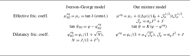

Figure 4. Comparison of the effective volume fractions proposed here
 $\varphi ^{\textit{eq}}$
in (2.10) and by Iverson and George
$\varphi ^{\textit{eq}}$
in (2.10) and by Iverson and George
 $\varphi ^{\textit{eq}}_{\textit{IG}}$
in (3.18e) as a function of the inertial number
$\varphi ^{\textit{eq}}_{\textit{IG}}$
in (3.18e) as a function of the inertial number
 $I$
for fixed
$I$
for fixed
 $J=10^{-1}, 10^{-2}, 10^{-3}$
and with values
$J=10^{-1}, 10^{-2}, 10^{-3}$
and with values
 $\alpha _\varphi =0.1, a_\varphi =0.66$
for
$\alpha _\varphi =0.1, a_\varphi =0.66$
for
 $\varphi ^{\textit{eq}}$
in (2.10).
$\varphi ^{\textit{eq}}$
in (2.10).
4. Models with two velocities in the mixture
4.1. Two-layer model with two velocities in the mixture (model B1)
The model B1 (see figure 3) is a simplification of the original full model A1 (§ 2.3) that is obtained by assuming that the upper fluid layer is no longer free but moves with the velocity of the mixture
 $\boldsymbol{v}_m$
:
$\boldsymbol{v}_m$
:
 \begin{align} \boldsymbol{u}_f=\boldsymbol{v}_m\equiv \frac {\rho _s\varphi \boldsymbol{v} + \rho _f(1-\varphi ) \boldsymbol{u}}{\rho }, \end{align}
with
 $\rho$
given by (2.1). This makes it possible to remove one velocity from the unknowns by assuming an infinite friction coefficient between the layers (
$\rho$
given by (2.1). This makes it possible to remove one velocity from the unknowns by assuming an infinite friction coefficient between the layers (
 $k_f\to \infty$
) in the original model (2.16)–(2.25). To eliminate
$k_f\to \infty$
) in the original model (2.16)–(2.25). To eliminate
 $k_f(\boldsymbol{u}_f-\boldsymbol{v}_m)$
in the momentum equations, we combine the fluid equations as follows: (2.18b)
$k_f(\boldsymbol{u}_f-\boldsymbol{v}_m)$
in the momentum equations, we combine the fluid equations as follows: (2.18b)
 $+ ({\rho _f(1-\varphi ))}/{\rho }\times$
(2.18c). We then write the system in a conservative form to obtain the two-velocity system for unknowns
$+ ({\rho _f(1-\varphi ))}/{\rho }\times$
(2.18c). We then write the system in a conservative form to obtain the two-velocity system for unknowns
 $h_m, h_f, \varphi, \boldsymbol{u}, \boldsymbol{v}$
(see supplementary material, § S.C.1). As for the full model A1, model B1 preserves the total mass and volume and the masses and volumes for each phase (see Bouchut et al. Reference Bouchut, Fernández-Nieto, Mangeney and Narbona-Reina2016).
$h_m, h_f, \varphi, \boldsymbol{u}, \boldsymbol{v}$
(see supplementary material, § S.C.1). As for the full model A1, model B1 preserves the total mass and volume and the masses and volumes for each phase (see Bouchut et al. Reference Bouchut, Fernández-Nieto, Mangeney and Narbona-Reina2016).
As we did in § 3.1.1 and to compare our model with the Meng–Wang model (Meng & Wang Reference Meng and Wang2018), we rewrite the above system (model B1) in terms of the virtual thickness
 $H$
and
$H$
and
 $\varDelta _H$
introduced in (2.3) and (2.4), respectively. For easy tracking in this section, we point out once again that
$\varDelta _H$
introduced in (2.3) and (2.4), respectively. For easy tracking in this section, we point out once again that
 \begin{align} h_m=H-\varDelta _H,\quad h_m+h_f=H+(h_f-\varDelta _H),\quad \rho _f h_f = \rho (H-h_m)=\rho \varDelta _H. \end{align}
From the mass equations in (S.C.1) (supplementary material), we obtain the total mass conservation equation
 \begin{equation} \partial _t(\rho H)+\nabla \cdot (\rho H \boldsymbol{v}_m)=0. \end{equation}
Each of the mass equations can also be written in terms of
 $H$
as follows (see supplementary material, § S.C.1 for details):
$H$
as follows (see supplementary material, § S.C.1 for details):
 \begin{equation} \partial _t (\rho _s\varphi H) + \nabla\cdot (\rho _s\varphi H \boldsymbol{v}) = -\varphi \frac {\rho _f\rho _s}{\rho }(H\Phi + \nabla\cdot (H(1-\varphi )(\boldsymbol{u}-\boldsymbol{v}))), \end{equation}
 \begin{equation} \partial _t (\rho _f(1-\varphi ) H) + \nabla\cdot (\rho _f(1-\varphi ) H \boldsymbol{u}) = \varphi \frac {\rho _f\rho _s}{\rho } (H\Phi + \nabla\cdot (H(1-\varphi )(\boldsymbol{u}-\boldsymbol{v}))), \end{equation}
 \begin{equation} \partial _t(\rho \varDelta _H)+\nabla\cdot (\rho \varDelta _H \boldsymbol{v}_m)=\rho _f \mathcal {V}_f. \end{equation}
The momentum equations given in (S.C.4a), (S.C.4b) (supplementary material) become
 \begin{align} &\partial _t\Big (\rho _s\varphi (H \boldsymbol{v}+\varDelta _H(\boldsymbol{v}_m-\boldsymbol{v})) \Big ) +\nabla \cdot \Big (\rho _s\varphi \left (H\boldsymbol{v}\otimes \boldsymbol{v}+\varDelta _H (\boldsymbol{v}_m\otimes \boldsymbol{v}_m -\boldsymbol{v}\otimes \boldsymbol{v})\right )\Big )\\ & = -g\cos \theta \nabla \left ((\rho _s-\rho _f)\varphi \frac {(H-\varDelta _H)^2}{2}+\rho _f\frac {(H+(h_f-\varDelta _H))^2}{2}\right )\nonumber \\ & +\rho _f(1-\varphi ) g\cos \theta H \nabla (H+(h_f-\varDelta _H)) -\rho _s \varphi H g\cos \theta \nabla b +(1-\varphi ) (H-\varDelta _H) \overline {\nabla p^e_{f_m}}\nonumber \\ & +\beta (H-\varDelta _H) (\boldsymbol{u}-\boldsymbol{v}) -\mu \mathop {\textrm {sgn}}(\boldsymbol{v}) \left (\varphi (\rho _s-\rho _f)g\cos \theta (H-\varDelta _H)-(p^e_{f_m})_{|b}\right )_+\nonumber \\ & +\frac {\rho _s \varphi }{\rho }((1-\lambda _f)\boldsymbol{u}+\lambda _f \boldsymbol{v}_m)\rho _f\mathcal {V}_f -\rho _s \varphi H g \sin\theta\; {\boldsymbol e}_x -\varDelta _H\frac {\rho _f\rho _s}{\rho } \boldsymbol{v}_m(\varphi \Phi +(\boldsymbol{v}-\boldsymbol{v}_m)\cdot \nabla \varphi ),\nonumber \end{align}
 \begin{align} & \partial _t\Big (\rho _f(1-\varphi ) (H \boldsymbol{u}+\varDelta _H(\boldsymbol{v}_m-\boldsymbol{u})) \Big ) +\nabla \!\cdot \Big (\rho _f(1-\varphi )\!\left (H\boldsymbol{u}\otimes \boldsymbol{u}+\varDelta _H (\boldsymbol{v}_m\otimes \boldsymbol{v}_m -\boldsymbol{u}\otimes \boldsymbol{u})\right )\!\!\Big )\nonumber\\ & = -\rho _f(1-\varphi ) H g\cos \theta \nabla (b+H+(h_f-\varDelta _H)) -(1-\varphi ) (H-\varDelta _H) \overline {\nabla p^e_{f_m}}\nonumber \\ & -\beta (H-\varDelta _H) (\boldsymbol{u}-\boldsymbol{v}) -\frac {\rho _s \varphi }{\rho }((1-\lambda _f)\boldsymbol{u}+\lambda _f \boldsymbol{v}_m)\rho _f\mathcal{V}_f -\frac 52\frac {\eta _e(1-\varphi )}{H-\varDelta _H}\boldsymbol{u}\nonumber \\ & -\rho _f (1-\varphi ) Hg \sin\theta\; {\boldsymbol e}_x +\varDelta _H \frac {\rho _f\rho _s}{\rho } \boldsymbol{v}_m(\varphi \Phi +(\boldsymbol{v}-\boldsymbol{v}_m)\cdot \nabla \varphi ), \end{align}
with
 \begin{equation} \mathcal {V}_f=-(H-\varDelta _H)\Phi -\nabla \cdot \big ((H-\varDelta _H)(1-\varphi )(\boldsymbol{u}-\boldsymbol{v})\big ). \end{equation}
In these equations, we can also use the following equivalence that relates the velocity differences:
 \begin{align} \rho _f(1-\varphi ) (\boldsymbol{u}-\boldsymbol{v}_m)=\rho _s \varphi (\boldsymbol{v}_m-\boldsymbol{v}) = \frac {\rho _f(1-\varphi )\rho _s \varphi }{\rho } (\boldsymbol{u}-\boldsymbol{v}). \end{align}
4.2. One-layer model with two velocities (model C1)
As we did for the one-velocity model C2, an oversimplified version (model C1) (see figure 3) of the two-layer model B1 may be obtained by using the virtual thickness
 $H$
as the only thickness. We thus assume the same condition as in (3.12),
$H$
as the only thickness. We thus assume the same condition as in (3.12),
 \begin{align} \varDelta _H = H-h_m \ll H, \end{align}
and obtain the following system for the unknowns
 $H,\varphi, \boldsymbol{u}, \boldsymbol{v}$
:
$H,\varphi, \boldsymbol{u}, \boldsymbol{v}$
:
 \begin{equation} \partial _t (\rho _s\varphi H) + \nabla\cdot (\rho _s\varphi H \boldsymbol{v}) = \varphi \frac {\rho _f\rho _s}{\rho }\mathcal V_f^*, \end{equation}
 \begin{equation} \partial _t (\rho _f(1-\varphi ) H) + \nabla\cdot (\rho _f(1-\varphi ) H \boldsymbol{u}) = -\varphi \frac {\rho _f\rho _s}{\rho } \mathcal V_f^*, \end{equation}
 \begin{align} \partial _t\Big (\rho _s\varphi H \boldsymbol{v} \Big ) +\nabla \cdot \Big (\rho _s\varphi H\boldsymbol{v}\otimes \boldsymbol{v}\Big ) &= -g\cos \theta \nabla \left (\rho _s\varphi \frac {H^2}{2}\right ) +g\cos \theta \rho _f\frac {H^2}{2} \nabla \varphi \nonumber \\ &\quad -\rho _s \varphi H g\cos \theta \nabla b +(1-\varphi ) H (\overline {\nabla p^e_{f_m}})^*+\beta H (\boldsymbol{u}-\boldsymbol{v})\nonumber \\ &\quad -\mathop {\textrm {sgn}}(\boldsymbol{v})\mu \left (\varphi (\rho _s-\rho _f)g\cos \theta H-(p^e_{f_m})_{|b}^*\right )_+\nonumber \\ &\quad +\frac {\rho _s \varphi }{\rho }((1-\lambda _f^*)\boldsymbol{u}+\lambda _f^* \boldsymbol{v}_m)\rho _f\mathcal {V}_f^*-\rho _s \varphi H g \textrm {sin} \theta {\boldsymbol e}_x, \end{align}
 \begin{align} \partial _t\Big (\rho _f(1-\varphi ) H \boldsymbol{u} \Big ) +\nabla \cdot \Big (\rho _f(1-\varphi ) H\boldsymbol{u}\otimes \boldsymbol{u}\Big ) &= -\rho _f(1-\varphi ) H g\cos \theta \nabla (b+H)\nonumber \\ &\quad -(1-\varphi ) H (\overline {\nabla p^e_{f_m}})^*-\beta H (\boldsymbol{u}-\boldsymbol{v})\nonumber \\ &\quad -\frac {\rho _s \varphi }{\rho }((1-\lambda _f^*)\boldsymbol{u}+\lambda _f^* \boldsymbol{v}_m)\rho _f\mathcal {V}_f^*\nonumber \\ &\quad -\frac 52\frac {\eta _e(1-\varphi )}{H}\boldsymbol{u}-\rho _f (1-\varphi ) Hg \textrm {sin} \theta {\boldsymbol e}_x. \end{align}
The rheological and dilatancy laws are modified in exactly the same way as for the one-layer model given by (3.14). The pressure term in the above momentum equations reads
 \begin{equation} (\overline {\nabla p^e_{f_m}})^*=\frac {1}{H}\Big ( \nabla (H (\overline p^e_{f_m})^*)+({p^e_{f_m}})_{|b}^*\nabla b\Big ) \qquad \mbox {with} \qquad (\overline p^e_{f_m})^*=-\frac {\beta }{(1-\varphi )^2}\frac {H^2}{3}\Phi ^*. \end{equation}
Note that this term does not appear in the one-layer model. Finally, the approximation the exchange term in (4.4f ) becomes
 \begin{equation} \mathcal {V}_f^*=-H\Phi ^*-\nabla \cdot \big (H(1-\varphi )(\boldsymbol{u}-\boldsymbol{v})\big ), \end{equation}
and the distribution coefficient
 $\lambda _f^*$
is defined as in (2.26) but with
$\lambda _f^*$
is defined as in (2.26) but with
 $\mathcal V_f^*$
:
$\mathcal V_f^*$
:
 \begin{equation} \lambda _f^*=\frac 12 -\frac 12 \mathop {\textrm {sgn}}(\mathcal {V}_f^*) \delta _f,\quad \delta _f=\left \{ \begin{array}{l} 0\quad \textrm {centered distribution,}\\ 1 \quad \textrm {upwind distribution.}\end{array}\right . \end{equation}
4.3. Comparison with the Meng–Wang model
In this section, we compare our previous one-layer two-velocity model C1 with the model proposed by Meng & Wang (Reference Meng and Wang2018). It comes from a combination of our previous work (Bouchut et al. Reference Bouchut, Fernández-Nieto, Mangeney and Narbona-Reina2016) and of the Iverson and George model (Iverson & George Reference Iverson and George2014; George & Iverson Reference George and Iverson2014). Indeed, they use the rheological and dilatancy laws from Bouchut et al. (Reference Bouchut, Fernández-Nieto, Mangeney and Narbona-Reina2016), as well as different fluid and solid velocities in the mixture, and they used our way of calculating the basal solid pressure. However, they use the virtual thickness concept of Iverson & George (Reference Iverson and George2014). As a result, as in the Iverson–George model, only the total mass
 $\rho h$
is conserved in the Meng–Wang model and there is no information on the conservation of the solid and the fluid mass or volume.
$\rho h$
is conserved in the Meng–Wang model and there is no information on the conservation of the solid and the fluid mass or volume.
4.3.1. Meng–Wang model
We express here the Meng–Wang model using our notation for the densities
 $\rho, \rho _s, \rho _f$
, velocities
$\rho, \rho _s, \rho _f$
, velocities
 $\boldsymbol{v}, \boldsymbol{u}$
and volume fraction
$\boldsymbol{v}, \boldsymbol{u}$
and volume fraction
 $\varphi$
, while we keep the notation
$\varphi$
, while we keep the notation
 $h$
for the virtual surface and
$h$
for the virtual surface and
 $p_e$
for the averaged excess pore pressure, as in the Iverson–George model (see equivalence of notation in the supplementary material, § S.E.2). We use the sub-index MW to denote particular coefficients for the Meng–Wang model. We have also recombined some terms in the equations for an easier comparison.
$p_e$
for the averaged excess pore pressure, as in the Iverson–George model (see equivalence of notation in the supplementary material, § S.E.2). We use the sub-index MW to denote particular coefficients for the Meng–Wang model. We have also recombined some terms in the equations for an easier comparison.
The Meng–Wang model for unknowns
 $h, \varphi, \boldsymbol{v}, \boldsymbol{u}$
is stated as
$h, \varphi, \boldsymbol{v}, \boldsymbol{u}$
is stated as
 \begin{equation} \partial _t(\rho _s\varphi h)+\nabla (\rho _s \varphi h\boldsymbol{v})={\mathfrak {J}}, \end{equation}
 \begin{equation} \partial _t(\rho _f(1-\varphi ) h)+\nabla (\rho _f (1-\varphi ) h\boldsymbol{u})=-\mathfrak {J}, \end{equation}
 \begin{align} &\partial _t (\rho _s\varphi h \boldsymbol{v})+\nabla \cdot ( \rho _s\varphi h\boldsymbol{v}\otimes \boldsymbol{v})= - \nabla \left (\rho _s\varphi g\cos \theta \frac {h^2}{2}\right )+ g\cos \theta \rho _f\frac {h^2}{2} \nabla \varphi \nonumber \\ &\quad +(1-\varphi )\nabla ( h p_e ) -\mathop {\textrm {sgn}}(\boldsymbol{v})\mu _{\textit{MW}}\Big (\varphi (\rho _s-\rho _f)hg\cos \theta -(p_e)_{|b}\Big ) \nonumber \\ &\quad +h\beta _{\textit{MW}}(\boldsymbol{u}-\boldsymbol{v})-\rho _s\varphi h g\sin \theta {\boldsymbol e}_x +((1-\lambda ) \boldsymbol{u}+\lambda \boldsymbol{v})\mathfrak {J} -\alpha _s \varphi \boldsymbol{v}, \end{align}
 \begin{eqnarray} \partial _t (\rho _f(1-\varphi ) h\boldsymbol{u})+\nabla \cdot (\rho _f(1-\varphi )h \boldsymbol{u}\otimes \boldsymbol{u})&=& -(1-\varphi )\nabla \left (\rho _f g\cos \theta \frac {h^2}{2}\right )\!,\,\, \end{eqnarray}
 \begin{align} & -(1-\varphi )\nabla ( h p_e) -\alpha _f (1-\varphi ) \boldsymbol{u}-h\beta _{\textit{MW}}(\boldsymbol{u}-\boldsymbol{v}) \nonumber \\ & -\rho _f(1-\varphi )h g\sin \theta {\boldsymbol e}_x -((1-\lambda ) \boldsymbol{u}+\lambda \boldsymbol{v})\mathfrak {J} \nonumber \\ & + h(1-\varphi )\nabla \cdot (2\eta _f D(\boldsymbol{u})). \end{align}
The granular mass flux
 $\mathfrak {J}$
through the virtual surface is given by
$\mathfrak {J}$
through the virtual surface is given by
 \begin{equation} \mathfrak {J}=-\varphi \frac {\rho _f\rho _s}{\rho }\Big (h\Phi _{\textit{MW}}+\nabla \cdot (h\, (1-\varphi )\, (\boldsymbol{u}-\boldsymbol{v}))\Big ), \end{equation}
and the value for
 $\Phi _{\textit{MW}}$
considered by Meng & Wang (Reference Meng and Wang2018) coincides with the one defined in (5.8) and (5.9) of Bouchut et al. (Reference Bouchut, Fernández-Nieto, Mangeney and Narbona-Reina2016), that is,
$\Phi _{\textit{MW}}$
considered by Meng & Wang (Reference Meng and Wang2018) coincides with the one defined in (5.8) and (5.9) of Bouchut et al. (Reference Bouchut, Fernández-Nieto, Mangeney and Narbona-Reina2016), that is,
 \begin{equation*} \Phi _{\textit{MW}} =\dot \gamma _{\textit{MW}}\tan \psi _{\textit{MW}},\quad \tan \psi _{\textit{MW}}=K_1(\varphi -\varphi ^{\textit{eq}}_{\textit{MW}}),\quad \varphi ^{\textit{eq}}_{\textit{MW}}=\varphi _c-K_2\frac {\eta _f \dot \gamma _{\textit{MW}}}{{p_s}_{|b}}, \end{equation*}
 \begin{equation} \dot \gamma _{\textit{MW}}=3\frac {|\boldsymbol{v}|}{h},\quad \mu _{\textit{MW}}=\tan (\delta + \psi _{\textit{MW}}), \end{equation}
for
 $\eta _f$
the dynamic viscosity of the fluid. The friction coefficient between phases is
$\eta _f$
the dynamic viscosity of the fluid. The friction coefficient between phases is
 \begin{equation} \beta _{\textit{MW}} = (1-\varphi )^2\frac {\eta _f}{k_{\textit{MW}}}, \end{equation}
where the hydraulic permeability
 $k_{\textit{MW}}$
is considered as a constant. The terms related to the pressure are
$k_{\textit{MW}}$
is considered as a constant. The terms related to the pressure are
 \begin{equation} p_e=\frac 23 (p_e)_{|b},\qquad (p_e)_{|b}=-\frac 12 \frac {\beta _{\textit{MW}}}{(1-\varphi )^2} h^2\Big (\Phi _{\textit{MW}}+\nabla \cdot ((1-\varphi )(\boldsymbol{u}-\boldsymbol{v}))\Big ). \end{equation}
The viscous term, the last term in (4.11d
), involves the strain rate
 $D(\boldsymbol{u})=(\nabla \boldsymbol{u}+\nabla ^t \boldsymbol{u})/2$
for
$D(\boldsymbol{u})=(\nabla \boldsymbol{u}+\nabla ^t \boldsymbol{u})/2$
for
 $\boldsymbol{u}$
the averaged fluid velocity. The coefficient
$\boldsymbol{u}$
the averaged fluid velocity. The coefficient
 $\lambda$
in the momentum equations arbitrarily determines the distribution of the granular mass flux between the phases at the virtual interface. It is given by Meng & Wang (Reference Meng and Wang2018) as
$\lambda$
in the momentum equations arbitrarily determines the distribution of the granular mass flux between the phases at the virtual interface. It is given by Meng & Wang (Reference Meng and Wang2018) as
 \begin{equation} \lambda =1-\varphi . \end{equation}
The friction coefficients
 $\alpha _s$
and
$\alpha _s$
and
 $\alpha _f$
are for the solid and fluid at the bottom, respectively. Strangely, two friction forces are considered for the solid at the bottom: the Coulomb friction and a Navier drag with coefficient
$\alpha _f$
are for the solid and fluid at the bottom, respectively. Strangely, two friction forces are considered for the solid at the bottom: the Coulomb friction and a Navier drag with coefficient
 $\alpha _s$
.
$\alpha _s$
.
4.3.2. Obtaining our model (model C1)
The Meng–Wang model (4.11) becomes our one-layer two-velocity model C1 (i.e. (4.7)) with
 $b=0$
under the following assumptions:
$b=0$
under the following assumptions:
-
(i)
$h=H$
; -
(ii)
$\nabla \cdot (2\eta _f D(\boldsymbol{u}))$
is negligible; -
(iii)
$\alpha _f= (5/2)({\eta _e}/{h_m})$
; -
(iv)
$\alpha _s=0$
(no additional Navier friction at the bottom for the solid phase).


Let us discuss the second and third assumptions related to the viscous and bottom friction stresses in the fluid. In the Meng–Wang model, the authors only kept the downslope gradient of the viscous stress tensor
 $\nabla \cdot (2\eta _f D(\boldsymbol{u}))$
and removed the slope perpendicular gradient that leads, when depth-averaged, to the viscous stress at the bottom
$\nabla \cdot (2\eta _f D(\boldsymbol{u}))$
and removed the slope perpendicular gradient that leads, when depth-averaged, to the viscous stress at the bottom
 $(5/2)({\eta _e \boldsymbol{u}}/{h_m})$
. This last term is however dominant in the asymptotics related to the shallow flow approximation. Furthermore, if the term
$(5/2)({\eta _e \boldsymbol{u}}/{h_m})$
. This last term is however dominant in the asymptotics related to the shallow flow approximation. Furthermore, if the term
 $\nabla \cdot (2\eta _f D(\boldsymbol{u}))$
is kept, other small terms of the same order should have been kept in the slope-perpendicular momentum equations. Instead of keeping the viscous stress at the bottom, they used the Navier friction law from Bouchut et al. (Reference Bouchut, Fernández-Nieto, Mangeney and Narbona-Reina2016). Replacing the constant value of
$\nabla \cdot (2\eta _f D(\boldsymbol{u}))$
is kept, other small terms of the same order should have been kept in the slope-perpendicular momentum equations. Instead of keeping the viscous stress at the bottom, they used the Navier friction law from Bouchut et al. (Reference Bouchut, Fernández-Nieto, Mangeney and Narbona-Reina2016). Replacing the constant value of
 $\alpha _f$
by the expression above results in replacing the Navier friction law by the basal viscous term (see supplementary material, § S.A.2). There are other differences coming from the considered closure relations. Details of calculations are given in the supplementary material, § S.B.2.1. The rheology in the Meng–Wang model is taken from Pailha & Pouliquen (Reference Pailha and Pouliquen2009) and Bouchut et al. (Reference Bouchut, Fernández-Nieto, Mangeney and Narbona-Reina2016), while we used updated rheology in the present work. The friction coefficient
$\alpha _f$
by the expression above results in replacing the Navier friction law by the basal viscous term (see supplementary material, § S.A.2). There are other differences coming from the considered closure relations. Details of calculations are given in the supplementary material, § S.B.2.1. The rheology in the Meng–Wang model is taken from Pailha & Pouliquen (Reference Pailha and Pouliquen2009) and Bouchut et al. (Reference Bouchut, Fernández-Nieto, Mangeney and Narbona-Reina2016), while we used updated rheology in the present work. The friction coefficient
 $\beta$
between the solid and fluid phases in the mixture is also different since the hydraulic permeability
$\beta$
between the solid and fluid phases in the mixture is also different since the hydraulic permeability
 $k_{\textit{MW}}$
is a constant, while our permeability depends on the grain diameter and on the solid volume fraction (see (2.21)). This is a key difference, as will be shown in the numerical tests. Another difference comes from the approximation of the basal pore pressure (compare (4.11i) for the Meng–Wang model and (3.14) in the present work). Indeed, they took the higher order approximation given by Bouchut et al. (Reference Bouchut, Fernández-Nieto, Mangeney and Narbona-Reina2016) corresponding to values of
$k_{\textit{MW}}$
is a constant, while our permeability depends on the grain diameter and on the solid volume fraction (see (2.21)). This is a key difference, as will be shown in the numerical tests. Another difference comes from the approximation of the basal pore pressure (compare (4.11i) for the Meng–Wang model and (3.14) in the present work). Indeed, they took the higher order approximation given by Bouchut et al. (Reference Bouchut, Fernández-Nieto, Mangeney and Narbona-Reina2016) corresponding to values of
 $\beta \sim \textit {O}(1)$
, while we only kept here the term corresponding to
$\beta \sim \textit {O}(1)$
, while we only kept here the term corresponding to
 $\beta \sim \textit {O}(\epsilon ^{-1})$
. Since
$\beta \sim \textit {O}(\epsilon ^{-1})$
. Since
 $\beta$
values are very high, we do not require an approximation of the basal pore pressure higher than
$\beta$
values are very high, we do not require an approximation of the basal pore pressure higher than
 $\beta \sim \textit {O}(\epsilon ^{-1})$
.
$\beta \sim \textit {O}(\epsilon ^{-1})$
.
Regarding the additional Navier solid friction, Meng et al. (Reference Meng, Wang, Wang and Fisher2017) assert that in the absence of such an additional friction term, the granular mass would be continuously accelerated. However, in the numerical comparison performed here (see § 5.3.1), this additional friction term has no significant effect. This lack of impact stems from the fact that Coulomb friction is proportional to the pressure, making it four orders of magnitude larger than this linear term.
To identify other differences between the Meng–Wang model and model C1, note that
 \begin{align} \mathfrak J = \varphi \frac {\rho _f \rho _s}{\rho } \mathcal V_f^* \qquad \mbox {and}\qquad \lambda = \frac {\varphi \rho _s}{\rho }\lambda _f^*. \end{align}
Note also that if we assume
 $\boldsymbol{u}=\boldsymbol{v}$
in the Meng–Wang model, we do not obtain the Iverson–George model since the closures for pressure, dilatancy and rheology are instead inspired by our previous work (Bouchut et al. Reference Bouchut, Fernández-Nieto, Mangeney and Narbona-Reina2016). Instead, we obtain a model similar to our oversimplified model C2 with the equivalence
$\boldsymbol{u}=\boldsymbol{v}$
in the Meng–Wang model, we do not obtain the Iverson–George model since the closures for pressure, dilatancy and rheology are instead inspired by our previous work (Bouchut et al. Reference Bouchut, Fernández-Nieto, Mangeney and Narbona-Reina2016). Instead, we obtain a model similar to our oversimplified model C2 with the equivalence
 $h=H$
(see (3.13)).
$h=H$
(see (3.13)).
5. Numerical illustrations in uniform regime
In this section, we perform a series of simulations of granular flows on sloping beds in uniform regimes to compare the series of models derived here between one another and with the Iverson–George and Meng–Wang models. We first consider, in § 5.1, immersed granular flows that mimic submarine avalanches to compare with the lab-experiments presented by Pailha & Pouliquen (Reference Pailha and Pouliquen2009). Then, in §§ 5.2,5.3, we focus on grain–fluid flows with a small layer of fluid on top of them, which are a proxy for natural debris flows. For the sake of clarity, the equations describing these uniform configurations for the different models (figure 3) are given in the supplementary material (§ S.D.1). Notice that since simulations are made in the 1-D configuration, the bold format is removed for velocity notations that now read
 $v$
,
$v$
,
 $u$
,
$u$
,
 $u_f$
,
$u_f$
,
 $v_m$
.
$v_m$
.
5.1. Immersed flows – effect of rheology
In this test, we compare the present rheology (2.10) to that used by Bouchut et al. (Reference Bouchut, Fernández-Nieto, Mangeney and Narbona-Reina2016) and discuss the sensitivity of the results to the rheological parameters by comparing with lab-experiments (Pailha & Pouliquen Reference Pailha and Pouliquen2009). These experiments correspond to the immersed configuration (see figure 2 of Bouchut et al. (Reference Bouchut, Fernández-Nieto, Mangeney and Narbona-Reina2016)), described by the following equations:
 \begin{equation} \partial _t h_m = h_m\Phi, \end{equation}
 \begin{equation} \partial _t \varphi = -\varphi \Phi, \end{equation}
 \begin{equation} \partial _t v = -\mu \mathop {\textrm {sgn}}(v) \frac {{p_s}_{|b}}{\rho _s \varphi h_m}+\frac {\beta }{\rho _s \varphi }(u-v) - g(1-\rho _f/\rho _s)\sin \theta {\boldsymbol e}_x, \end{equation}
 \begin{equation} \partial _t u = -\frac 12 \Phi \frac {u}{1-\varphi } -\frac {\beta }{\rho _f (1-\varphi )}(u-v) -\frac {k_b}{\rho _f(1-\varphi ) h_m } u, \end{equation}
with
 $k_b=(5/2) \eta _e(1-\varphi )/h_m$
, which is a very small term in all the simulations. To be consistent with Bouchut et al. (Reference Bouchut, Fernández-Nieto, Mangeney and Narbona-Reina2016), we neglect the friction between the mixture and the upper-fluid layer by setting
$k_b=(5/2) \eta _e(1-\varphi )/h_m$
, which is a very small term in all the simulations. To be consistent with Bouchut et al. (Reference Bouchut, Fernández-Nieto, Mangeney and Narbona-Reina2016), we neglect the friction between the mixture and the upper-fluid layer by setting
 $k_f=0$
in (2.19) and we consider the centred distribution in (2.26),
$k_f=0$
in (2.19) and we consider the centred distribution in (2.26),
 $\lambda _f=1/2$
. Note that in this test, we do not study the effect of the upper-fluid layer since the free surface is fixed to be horizontal and only
$\lambda _f=1/2$
. Note that in this test, we do not study the effect of the upper-fluid layer since the free surface is fixed to be horizontal and only
 $h_m$
is solved.
$h_m$
is solved.
5.1.1. Physical and rheological parameters
Following Pailha & Pouliquen (Reference Pailha and Pouliquen2009) and Bouchut et al. (Reference Bouchut, Fernández-Nieto, Mangeney and Narbona-Reina2016), four cases are analysed, corresponding to loose and dense initial packing volume fraction, both for high and low fluid viscosity. For all of them, we use
 \begin{align} \rho _s=2500 \, \mbox {kg m}^{-3}, \quad \rho _f = 1041 \, \mbox {kg m}^{-3}, \quad d=1.6 \times 10^{-4} \, \mbox {m}. \end{align}
The high viscosity case corresponds to
 $\eta _f=0.96 \times 10^{-1}$
Pa s, a slope angle
$\eta _f=0.96 \times 10^{-1}$
Pa s, a slope angle
 $\theta =25^o$
and
$\theta =25^o$
and
 \begin{align} h_m^0=4.9 \times 10^{-3} \, \mbox {m}, \quad \varphi ^0=\left \{\begin{array}{ll} 0.562 & \mbox {loose}, \\0.588 & \mbox {dense}, \end{array}\right . \quad u^0=v^0=0 \, \mbox {m}\, \mbox {s}^{-1}. \end{align}
The low viscosity case corresponds to
 $\eta _f=0.98 \times 10^{-2}$
Pa s, a slope angle
$\eta _f=0.98 \times 10^{-2}$
Pa s, a slope angle
 $\theta =28^o$
with
$\theta =28^o$
with
 \begin{align} h_m^0=6.1 \times 10^{-3} \, \mbox {m}, \quad \varphi ^0=\left \{\begin{array}{ll} 0.576 & \mbox {loose}, \\0.592 & \mbox {dense}, \end{array}\right . \quad u^0=v^0=0 \, \mbox {m} \,\mbox {s}^{-1}, \end{align}
where
 $u^0$
and
$u^0$
and
 $v^0$
are the initial fluid and solid velocities within the mixture. Finally, the parameters defining the rheological laws, see (2.10), are
$v^0$
are the initial fluid and solid velocities within the mixture. Finally, the parameters defining the rheological laws, see (2.10), are
 $\alpha _\varphi$
,
$\alpha _\varphi$
,
 $\alpha _\mu$
,
$\alpha _\mu$
,
 $\varphi _c$
,
$\varphi _c$
,
 $\mu _c$
,
$\mu _c$
,
 $I_0$
,
$I_0$
,
 $b_\varphi$
and
$b_\varphi$
and
 $\Delta \mu$
. For the first two parameters involved in the definition of
$\Delta \mu$
. For the first two parameters involved in the definition of
 ${\mathcal {J}}_\varphi$
and
${\mathcal {J}}_\varphi$
and
 ${\mathcal {J}}_\mu$
, respectively, we use the values of Tapia et al. (Reference Tapia, Ichihara, Pouliquen and Guazzelli2022)
${\mathcal {J}}_\mu$
, respectively, we use the values of Tapia et al. (Reference Tapia, Ichihara, Pouliquen and Guazzelli2022)
 \begin{align} \alpha _\varphi =0.1, \quad \alpha _\mu =0.0088 \end{align}
since such parameters did not appear in the rheology chosen by Pailha & Pouliquen (Reference Pailha and Pouliquen2009) where the lab-experiments were presented. As in Pailha & Pouliquen (Reference Pailha and Pouliquen2009), we set
 \begin{align} \varphi _c=0.582, \quad \mu _c=0.415\quad \mbox {and} \quad I_0=0.279. \end{align}
Finally, we must specify the values of
 $b_\varphi$
and
$b_\varphi$
and
 $\Delta \mu$
. To be as close as possible to the rheology of Tapia et al. (Reference Tapia, Ichihara, Pouliquen and Guazzelli2022) (table 2), that is,
$\Delta \mu$
. To be as close as possible to the rheology of Tapia et al. (Reference Tapia, Ichihara, Pouliquen and Guazzelli2022) (table 2), that is,
 \begin{equation} \varphi ^{\textit{eq}}_{\textit{Tapia}}=\varphi _c (1-a_\varphi \mathcal {J}_\varphi ^{1/2}),\qquad \mu ^{\textit{eq}}_{\textit{Tapia}}=\mu _c (1+a_\mu \mathcal {J}_\mu ^{1/2}), \end{equation}
we linearise our expressions (2.10) as follows:
 \begin{equation} \varphi ^{\textit{eq}}_{\textit{lin}} = \varphi _c-\varphi _c b_\varphi \mathcal {J}_\varphi ^{1/2}, \qquad \mu ^{\textit{eq}}_{\textit{lin}}s = \mu _c+\frac {\Delta \mu }{I_0} \mathcal {J}_\mu ^{1/2}. \end{equation}
By comparing (5.7) and (5.8), we obtain the following equivalence of parameters:
 \begin{align} b_\varphi \equiv a_\varphi, \qquad \Delta \mu \equiv \mu _c I_0 a_\mu . \end{align}
Tapia et al. (Reference Tapia, Ichihara, Pouliquen and Guazzelli2022) proposed the values
 $a_\varphi =0.66$
,
$a_\varphi =0.66$
,
 $a_\mu =11.29$
to fit their laboratory experiments, thus leading to
$a_\mu =11.29$
to fit their laboratory experiments, thus leading to
 \begin{align} b_\varphi =a_\varphi =0.66, \quad \Delta \mu =\mu _c I_0 a_\mu, \quad \mbox {with} \quad a_\mu =11.29. \end{align}
Finally, we perform a sensitivity analysis around these values to identify the set of parameters making it possible to obtain the steady states with our present rheology that are as close as possible to that used by Bouchut et al. (Reference Bouchut, Fernández-Nieto, Mangeney and Narbona-Reina2016) (see supplementary material, § S.D.3). Based on this analysis, we set
 \begin{align} \Delta \mu =0.653, \qquad b_\varphi =0.99, \end{align}
corresponding to
 $a_\mu =5.645$
.
$a_\mu =5.645$
.
We focus here on the analysis of the effect of using different rheologies since the characteristics of the flow behaviour in loose and dense cases have been already studied by Bouchut et al. (Reference Bouchut, Fernández-Nieto, Mangeney and Narbona-Reina2016). In any case, we refer the reader to the supplementary material, § S.D.2 for a brief description of this behaviour.

Figure 5. Solid velocity
 $v$
, basal excess pore pressure
$v$
, basal excess pore pressure
 $(p^e_{f_m})_{|b}$
, solid volume fraction
$(p^e_{f_m})_{|b}$
, solid volume fraction
 $\varphi$
, friction coefficient
$\varphi$
, friction coefficient
 $\mu$
and tangent of the dilation angle
$\mu$
and tangent of the dilation angle
 $\psi$
in the (a,c,e,g) high viscosity and (b,d,f,h) low viscosity case, for both the dense (full lines) and the loose (dashed lines) cases. The results for the proposed rheology are in black/grey and for the rheology of Bouchut et al. (Reference Bouchut, Fernández-Nieto, Mangeney and Narbona-Reina2016) in blue. The lab-experiments from Pailha et al. (Reference Pailha, Nicolas and Pouliquen2008) are in green.
$\psi$
in the (a,c,e,g) high viscosity and (b,d,f,h) low viscosity case, for both the dense (full lines) and the loose (dashed lines) cases. The results for the proposed rheology are in black/grey and for the rheology of Bouchut et al. (Reference Bouchut, Fernández-Nieto, Mangeney and Narbona-Reina2016) in blue. The lab-experiments from Pailha et al. (Reference Pailha, Nicolas and Pouliquen2008) are in green.
5.1.2. Influence of the rheology
Figure 5 also makes it possible to compare the variables calculated with the rheology proposed here, the rheology used by Bouchut et al. (Reference Bouchut, Fernández-Nieto, Mangeney and Narbona-Reina2016) and the experimental data (Pailha & Pouliquen Reference Pailha and Pouliquen2009). At low viscosity, the present rheology better fits the experiments for the solid velocity and the basal excess pore pressure, in both the so-called loose and dense cases (figure 5
b,d). At high viscosity, the solid velocity with the present rheology is also closer to observations in the loose case (figure 5
a). The maximum velocity with the proposed rheology is two times higher than with the rheology of Bouchut et al. (Reference Bouchut, Fernández-Nieto, Mangeney and Narbona-Reina2016). In the dense case, the excess pore pressure is closer to the measurements with the rheology of Bouchut et al. (Reference Bouchut, Fernández-Nieto, Mangeney and Narbona-Reina2016) at the beginning, but its overall shape is better captured by the present rheology (figure 5
c). The greatest difference between the values of
 $(p^e_{f_m})_{|b}$
and
$(p^e_{f_m})_{|b}$
and
 $\varphi$
calculated with the two rheologies is observed in the dense case, while they are very close in the loose case. Concerning the friction coefficient, the critical-state friction coefficient
$\varphi$
calculated with the two rheologies is observed in the dense case, while they are very close in the loose case. Concerning the friction coefficient, the critical-state friction coefficient
 $\mu ^{\textit{eq}}$
is constant for Bouchut et al. (Reference Bouchut, Fernández-Nieto, Mangeney and Narbona-Reina2016), i.e. it does not depend on the viscous–inertial number (this dependency was replaced by a viscous term that depends on
$\mu ^{\textit{eq}}$
is constant for Bouchut et al. (Reference Bouchut, Fernández-Nieto, Mangeney and Narbona-Reina2016), i.e. it does not depend on the viscous–inertial number (this dependency was replaced by a viscous term that depends on
 $\dot {\gamma }$
). In the dense case, the time
$\dot {\gamma }$
). In the dense case, the time
 $t_{start}$
at which the granular layer starts to move is better reproduced by the rheology used by Bouchut et al. (Reference Bouchut, Fernández-Nieto, Mangeney and Narbona-Reina2016) but, afterwards, its evolution seems to be better captured with the present rheology.
$t_{start}$
at which the granular layer starts to move is better reproduced by the rheology used by Bouchut et al. (Reference Bouchut, Fernández-Nieto, Mangeney and Narbona-Reina2016) but, afterwards, its evolution seems to be better captured with the present rheology.
In figure 6, we investigate the influence of the rheological parameters
 $\Delta \mu$
and
$\Delta \mu$
and
 $b_\varphi$
on the flow variables for the two viscosities. For all cases, we observe that
$b_\varphi$
on the flow variables for the two viscosities. For all cases, we observe that
 $\Delta \mu$
controls the long-term steady-state velocity even though the long-term values of
$\Delta \mu$
controls the long-term steady-state velocity even though the long-term values of
 $\varphi$
are also controlled by
$\varphi$
are also controlled by
 $b_{\varphi }$
. In the dense and loose cases, the initial value of the velocity is also significantly affected by
$b_{\varphi }$
. In the dense and loose cases, the initial value of the velocity is also significantly affected by
 $b_\varphi$
. This would be expected since the compression/dilation mainly occurs during the first stage of the flow until approximately 300 s for high viscosity and 20 s for low viscosity. However, this tendency is not observed for the other variables. For example, in the dense case, it is rather
$b_\varphi$
. This would be expected since the compression/dilation mainly occurs during the first stage of the flow until approximately 300 s for high viscosity and 20 s for low viscosity. However, this tendency is not observed for the other variables. For example, in the dense case, it is rather
 $\Delta \mu$
that controls the first stage of variation of the excess pore fluid pressure and the absolute value of its maximum, the solid volume fraction
$\Delta \mu$
that controls the first stage of variation of the excess pore fluid pressure and the absolute value of its maximum, the solid volume fraction
 $\varphi$
, and the friction coefficient
$\varphi$
, and the friction coefficient
 $\mu$
. This is also the case for
$\mu$
. This is also the case for
 $\mu ^{\textit{eq}}$
,
$\mu ^{\textit{eq}}$
,
 $h_m$
and
$h_m$
and
 $\textrm {div}\, v$
but not for
$\textrm {div}\, v$
but not for
 $\tan \psi$
and
$\tan \psi$
and
 $\dot {\gamma }$
, not represented here. In the loose case, the variables are significantly different for the different values of
$\dot {\gamma }$
, not represented here. In the loose case, the variables are significantly different for the different values of
 $\Delta \mu$
and
$\Delta \mu$
and
 $b_\varphi$
, right from the start.
$b_\varphi$
, right from the start.

Figure 6. Test 1: solid velocity
 $v$
, basal excess pore pressure (
$v$
, basal excess pore pressure (
 ${p^e_{f_m}}_{|b}$
), solid volume fraction
${p^e_{f_m}}_{|b}$
), solid volume fraction
 $\varphi$
, friction coefficient
$\varphi$
, friction coefficient
 $\mu$
and tangent of the dilatancy angle
$\mu$
and tangent of the dilatancy angle
 $\psi$
, for (a,c,e,g) high viscosity and (b,d,f,h) low viscosity, and different values of
$\psi$
, for (a,c,e,g) high viscosity and (b,d,f,h) low viscosity, and different values of
 $\Delta \mu$
and
$\Delta \mu$
and
 $b_\varphi$
.
$b_\varphi$
.
After this first transient regime (
 ${\gt } 300$
s for high viscosity and
${\gt } 300$
s for high viscosity and
 ${\gt } 20$
s for low viscosity), the long-term values of the quantities are different for the different values of
${\gt } 20$
s for low viscosity), the long-term values of the quantities are different for the different values of
 $\Delta \mu$
and
$\Delta \mu$
and
 $b_\varphi$
for both the loose and dense cases. As observed above, the behaviour of the friction coefficient
$b_\varphi$
for both the loose and dense cases. As observed above, the behaviour of the friction coefficient
 $\mu$
is very similar to that of the excess pore fluid pressure, as these quantities are related (see § 2.4.3). In the dense case, the time needed for the mass to start moving
$\mu$
is very similar to that of the excess pore fluid pressure, as these quantities are related (see § 2.4.3). In the dense case, the time needed for the mass to start moving
 $t_{start}$
increases with increasing
$t_{start}$
increases with increasing
 $\Delta \mu$
as the friction increases. For the same
$\Delta \mu$
as the friction increases. For the same
 $\Delta \mu$
,
$\Delta \mu$
,
 $t_{start}$
increases with increasing
$t_{start}$
increases with increasing
 $b_\varphi$
.
$b_\varphi$
.
As a result, the dependency of the variables on the rheological parameters is significant and very complex, showing the high sensitivity of the model to the rheological parameters, which are often difficult to constrain on the field scale.
5.2. Debris flow configuration
For the following tests, we consider grain–fluid flows with a free surface in the configuration shown in figure 1, mimicking the experiment developed by Iverson et al. (Reference Iverson, Reid, Iverson, LaHusen, Logan, Mann and Brien2000) and simulated by George & Iverson (Reference George and Iverson2014). In this set-up, we compare the results from the series of models presented above, schematically represented in figure 3. For two-layer models, we define the thickness of the initial fluid-only layer at the top as a fraction
 $C_h$
of the mixture thickness
$C_h$
of the mixture thickness
 $h_f^0=C_h h_m^0$
.
$h_f^0=C_h h_m^0$
.
We set the following initial data:
 \begin{align} h_m^0=\left \{\begin{array}{ll} 0.7169 \,\mbox {m} & \mbox {loose}, \\0.65 \,\mbox {m} & \mbox {dense}, \end{array}\right . \ \varphi ^0=\left \{\begin{array}{ll} 0.48 & \mbox {loose}, \\0.59 & \mbox {dense}, \end{array}\right . \ h_f^0=C_h h_m^0 \, \mbox {m};\ u^0=v^0=u_f^0=0 \, \mbox {m} \mbox {s}^{-1}, \end{align}
with the slope angle of the bottom at
 $\theta =13^\circ$
for the so-called loose and
$\theta =13^\circ$
for the so-called loose and
 $\theta =20^\circ$
for the dense cases. We consider the same mass for the mixture in the loose and dense cases so that
$\theta =20^\circ$
for the dense cases. We consider the same mass for the mixture in the loose and dense cases so that
 $(\rho ^0 h_m^0)_{\textrm {loose}}=(\rho ^0 h_m^0)_{\textrm {dense}}$
. For one-layer models, the virtual thickness is
$(\rho ^0 h_m^0)_{\textrm {loose}}=(\rho ^0 h_m^0)_{\textrm {dense}}$
. For one-layer models, the virtual thickness is
 $H^0=h_m^0+\rho _f h_f^0/\rho ^0$
, where
$H^0=h_m^0+\rho _f h_f^0/\rho ^0$
, where
 $\rho ^0=\varphi ^0\rho _s+(1-\varphi ^0)\rho _f$
(see (2.1)). When the relaxation equation is used to solve the basal pressure, we assume that the excess pore pressure is zero at the beginning. As a result, the initial basal solid pressure is the hydrostatic pressure
$\rho ^0=\varphi ^0\rho _s+(1-\varphi ^0)\rho _f$
(see (2.1)). When the relaxation equation is used to solve the basal pressure, we assume that the excess pore pressure is zero at the beginning. As a result, the initial basal solid pressure is the hydrostatic pressure
 $p_{s_b}^0=\varphi ^0(\rho _s-\rho _f)g\cos \theta h_m^0$
for two-layer models and
$p_{s_b}^0=\varphi ^0(\rho _s-\rho _f)g\cos \theta h_m^0$
for two-layer models and
 $p_{s_b}^0=\varphi ^0(\rho _s-\rho _f)g\cos \theta H^0$
for one-layer models and for the Iverson–George model. In this last case, the relaxation coefficient is
$p_{s_b}^0=\varphi ^0(\rho _s-\rho _f)g\cos \theta H^0$
for one-layer models and for the Iverson–George model. In this last case, the relaxation coefficient is
 $\alpha =10^{-9}$
.
$\alpha =10^{-9}$
.
The material properties are
 \begin{align} \rho _f=1000\,\mbox {kg m}^{-3}, \quad \rho _s=2700\,\mbox {kg m}^{-3},\quad d=10^{-3}\,\mbox {m},\quad \eta _f=10^{-3}\, \mbox {Pa s}, \end{align}
and the rheological parameters
 \begin{equation*} \alpha _\varphi =0.1, \quad \alpha _\mu =0.0088, \quad b_\varphi =0.99,\quad I_0=0.279, \end{equation*}
 \begin{equation} \mu _c=\tan 29^\circ, \quad \varphi _c=0.56, \quad a_\mu =5.645, \quad \Delta \mu =\mu _c a_\mu I_0. \end{equation}
Finally, we set
 $m_f=1$
for the friction between the mixture and upper-fluid layer (see (2.19)).
$m_f=1$
for the friction between the mixture and upper-fluid layer (see (2.19)).
5.3. Comparison among all the proposed models for debris flows
We will focus here on the differences between the models of various levels of complexity for both loose and dense cases. The configuration and parameters are the same as those described in § 5.2. To provide deeper insight into the flow behaviour, we compute the forces involved in the model, given by the different terms in the equations. These forces are specified in table S1 of the supplementary material, § S.D.5, for models written in conservative form. Note that for the two-phase models, the forces are plotted for the mixture layer by summing up the momentum equations for the solid and fluid phases.
5.3.1. One-layer models compared with Iverson–George and Meng–Wang models
Let us compare, in the uniform regime, our one-layer model C2, presented in § 3.2, and model C1, presented in § 4.2 with the Iverson–George and Meng–Wang models, respectively. All these models are defined in terms of a virtual thickness. The equations of these models in the uniform regime are given in the supplementary material, § S.D.1: (S.D.12) for model C2, (S.D.16) for Iverson–George, (S.D.11) for model C1 and (S.D.18) for Meng–Wang. We choose the loose case with data given in § 5.2 and
 $C_h=0.15$
. The values of the constants involved in the Meng–Wang model are those given in their paper (Meng & Wang Reference Meng and Wang2018),
$C_h=0.15$
. The values of the constants involved in the Meng–Wang model are those given in their paper (Meng & Wang Reference Meng and Wang2018),
 \begin{align} K_1=1.1, \quad K_2=3,\quad \alpha _s=10\; \mbox {Ns m}^{-3},\quad \alpha _f=35\; \mbox {Ns m}^{-3}. \end{align}
For these models, the main difference lies in the rheological laws and in the definition of the permeability, which plays a key role, in particular, in the dilatancy function
 $\Phi$
in our model,
$\Phi$
in our model,
 $\Phi _{\textit{MW}}$
in the Meng–Wang model and
$\Phi _{\textit{MW}}$
in the Meng–Wang model and
 $D$
in the Iverson–George model. It has a strong impact on the excess pore pressure and therefore on the basal solid pressure. In our model, the permeability
$D$
in the Iverson–George model. It has a strong impact on the excess pore pressure and therefore on the basal solid pressure. In our model, the permeability
 $k$
is a function of
$k$
is a function of
 $\varphi$
and
$\varphi$
and
 $d$
the mean grain diameter. In the Iverson–George model,
$d$
the mean grain diameter. In the Iverson–George model,
 $k_{\textit{IG}}$
is a function of
$k_{\textit{IG}}$
is a function of
 $\varphi$
, and in the Meng–Wang model,
$\varphi$
, and in the Meng–Wang model,
 $k_{\textit{MW}}$
is assumed to be constant:
$k_{\textit{MW}}$
is assumed to be constant:
 \begin{align} k=\frac {(1-\varphi )^3d^2}{150 \varphi ^2},\quad k_{\textit{IG}}=k_0 \textrm{e}^{\frac {0.6-\varphi }{0.04}}, \quad k_{\textit{MW}}=10^{-9}\,\mbox {m}^2, \end{align}
with
 $k_0\in 10^{-13}-10^{-10}$
m
$k_0\in 10^{-13}-10^{-10}$
m
 $^2$
a reference permeability. In figure S14 in the supplementary material, we reproduce figure 5 of Iverson & George (Reference Iverson and George2014) for a value of the grain diameter
$^2$
a reference permeability. In figure S14 in the supplementary material, we reproduce figure 5 of Iverson & George (Reference Iverson and George2014) for a value of the grain diameter
 $d$
that makes it possible to fit experimental data. Note also that the range of values of the permeability
$d$
that makes it possible to fit experimental data. Note also that the range of values of the permeability
 $k$
is smaller than that for the permeability defined by
$k$
is smaller than that for the permeability defined by
 $k_{\textit{IG}}$
. Depending on the value of the constants
$k_{\textit{IG}}$
. Depending on the value of the constants
 $d$
,
$d$
,
 $k_0$
and
$k_0$
and
 $k_{\textit{MW}}$
, very different solutions are obtained, the models being highly sensitive to the permeability, as also discussed by Iverson & George (Reference Iverson and George2014). To illustrate this sensitivity, we test two values of
$k_{\textit{MW}}$
, very different solutions are obtained, the models being highly sensitive to the permeability, as also discussed by Iverson & George (Reference Iverson and George2014). To illustrate this sensitivity, we test two values of
 $k_0$
(
$k_0$
(
 $k_0=2.6\times 10^{-11}$
considered by George & Iverson (Reference George and Iverson2014) and
$k_0=2.6\times 10^{-11}$
considered by George & Iverson (Reference George and Iverson2014) and
 $k_0=5\times 10^{-10}$
) and two values of
$k_0=5\times 10^{-10}$
) and two values of
 $k_{\textit{MW}}$
(
$k_{\textit{MW}}$
(
 $k_{\textit{MW}}=10^{-9}$
and
$k_{\textit{MW}}=10^{-9}$
and
 $3\times 10^{-9}$
m
$3\times 10^{-9}$
m
 $^2$
). Figure 7(a) shows that the permeability obtained with the original values proposed for the Iverson–George model and the Meng–Wang model are quite far from the permeability
$^2$
). Figure 7(a) shows that the permeability obtained with the original values proposed for the Iverson–George model and the Meng–Wang model are quite far from the permeability
 $k$
, especially
$k$
, especially
 $k_{\textit{IG}}$
that is one order of magnitude smaller. This induces strong differences between the calculated mixture velocity
$k_{\textit{IG}}$
that is one order of magnitude smaller. This induces strong differences between the calculated mixture velocity
 $\boldsymbol{v}_m$
and basal solid pressure (figure 7
b). Our models C1 and C2 give almost the same results (the blue and the green lines are superimposed) because the solid and fluid velocities in the mixture become very close from the very beginning (figure 7
b). With the proposed models C1 and C2, the maximum velocity is approximately 5 m s–1, while it reaches 80 m s–1 in the Iverson–George model and 15 m s-1 in the Meng–Wang model. The mass stops much later given that the maximum velocity increases. The velocity increases in the same way in all models, but its decrease is controlled by the basal frictional shear stress, and thus the basal solid pressure and the friction coefficient. Indeed, the velocity increases when
$\boldsymbol{v}_m$
and basal solid pressure (figure 7
b). Our models C1 and C2 give almost the same results (the blue and the green lines are superimposed) because the solid and fluid velocities in the mixture become very close from the very beginning (figure 7
b). With the proposed models C1 and C2, the maximum velocity is approximately 5 m s–1, while it reaches 80 m s–1 in the Iverson–George model and 15 m s-1 in the Meng–Wang model. The mass stops much later given that the maximum velocity increases. The velocity increases in the same way in all models, but its decrease is controlled by the basal frictional shear stress, and thus the basal solid pressure and the friction coefficient. Indeed, the velocity increases when
 $p_{s|b}$
is almost zero, because of the high excess pore pressure, and decreases when
$p_{s|b}$
is almost zero, because of the high excess pore pressure, and decreases when
 $p_{s|b}$
returns to hydrostatic pressure. For example,
$p_{s|b}$
returns to hydrostatic pressure. For example,
 $p_{s|b}$
stays very low for a very long time in the Iverson–George model leading to this huge velocity.
$p_{s|b}$
stays very low for a very long time in the Iverson–George model leading to this huge velocity.

Figure 7. Comparison between our one-layer models C1 = [1L:
 ${(u,v)}$
] and C2 = [1L:
${(u,v)}$
] and C2 = [1L:
 ${(v)}$
] (lines are superimposed) and with the Iverson–George (IG) and Meng–Wang (MW) models. (a) Permeability for each model with two values of
${(v)}$
] (lines are superimposed) and with the Iverson–George (IG) and Meng–Wang (MW) models. (a) Permeability for each model with two values of
 $k_0$
in the Iverson–George model and of
$k_0$
in the Iverson–George model and of
 $k_{\textit{MW}}$
in the Meng–Wang model; (b) velocity.
$k_{\textit{MW}}$
in the Meng–Wang model; (b) velocity.
In view of these results, we compare the models under the same value of the permeability, choosing
 $k= ({(1-\varphi )^3d^2})/({150 \varphi ^2})$
obtained with
$k= ({(1-\varphi )^3d^2})/({150 \varphi ^2})$
obtained with
 $d=10^{-3}$
m. Results are shown in figure 8. Same permeability leads to very similar velocities and basal solid pressure (figure 8
a) for all models. Interestingly the Iverson–George model leads to a higher basal solid pressure than in our model but to a lower friction coefficient so that the velocities of the two models are very similar. The variation of the friction coefficient can only be observed at the very first instants (
$d=10^{-3}$
m. Results are shown in figure 8. Same permeability leads to very similar velocities and basal solid pressure (figure 8
a) for all models. Interestingly the Iverson–George model leads to a higher basal solid pressure than in our model but to a lower friction coefficient so that the velocities of the two models are very similar. The variation of the friction coefficient can only be observed at the very first instants (
 ${\lt } 3$
s), as shown in figure 8(b). Even if the velocities are similar, the friction coefficient
${\lt } 3$
s), as shown in figure 8(b). Even if the velocities are similar, the friction coefficient
 $\mu$
and the dilatancy
$\mu$
and the dilatancy
 $\tan \psi$
are not so close, because of the differences in the rheology.
$\tan \psi$
are not so close, because of the differences in the rheology.
Note that for the same permeability and rheology, the results obtained for the Iverson–George and C2 model pair, and the the Meng–Wang and C1 model pair are equivalent. For this reason, in the following, we perform the comparison only between the proposed models A, B and C.

Figure 8. Comparison between our one layer models C1 = [1L:
 ${(u,v)}$
] and C2 = [1L:
${(u,v)}$
] and C2 = [1L:
 ${(v)}$
] (lines are superimposed) and with the Iverson–George (IG) and Meng–Wang (MW) models for the same permeability
${(v)}$
] (lines are superimposed) and with the Iverson–George (IG) and Meng–Wang (MW) models for the same permeability
 $k={(1-\varphi )^3d^2}/{150 \varphi ^2}$
obtained with
$k={(1-\varphi )^3d^2}/{150 \varphi ^2}$
obtained with
 $d=10^{-3}$
m. (a) Basal solid pressure and velocity; (b) friction coefficient and dilatancy angle.
$d=10^{-3}$
m. (a) Basal solid pressure and velocity; (b) friction coefficient and dilatancy angle.

Figure 9. Loose case with slope angle
 $\theta =13^\circ$
and for
$\theta =13^\circ$
and for
 $C_h=0.15$
. Comparison between all the models: those accounting for two velocities
$C_h=0.15$
. Comparison between all the models: those accounting for two velocities
 $u,v$
in the mixture (models A1, B1 and C1) and those assuming
$u,v$
in the mixture (models A1, B1 and C1) and those assuming
 $u=v$
(models A2, B2 and C2), for two grain diameters (i.e. two permeabilities): (a,c,e,g)
$u=v$
(models A2, B2 and C2), for two grain diameters (i.e. two permeabilities): (a,c,e,g)
 $d=10^{-3}$
m and (b,d,f,h)
$d=10^{-3}$
m and (b,d,f,h)
 $d=10^{-2}$
m. (a,b) Mixture velocity; (c,d) all velocities; (e,f) basal solid pressure
$d=10^{-2}$
m. (a,b) Mixture velocity; (c,d) all velocities; (e,f) basal solid pressure
 ${p_s}_{|b}$
with basal excess pore pressure
${p_s}_{|b}$
with basal excess pore pressure
 $(p^e_{f_m})_{|b}$
; (g,h) friction coefficient
$(p^e_{f_m})_{|b}$
; (g,h) friction coefficient
 $\mu$
with dilatancy
$\mu$
with dilatancy
 $\tan \psi$
.
$\tan \psi$
.
5.3.2. Influence of grain diameter and drag force between the layers
We impose here
 $C_h=0.15$
and compare the results for two values of the mean grain diameter
$C_h=0.15$
and compare the results for two values of the mean grain diameter
 $d=10^{-3}$
m (figure 9
a,c,e,g) and
$d=10^{-3}$
m (figure 9
a,c,e,g) and
 $d=10^{-2}$
m (figure 9
b,d,f,h), for which the permeability is 100 times bigger (see (2.21)). Our first objective is to compare the models, denoted 1, that account for different solid and fluid velocities
$d=10^{-2}$
m (figure 9
b,d,f,h), for which the permeability is 100 times bigger (see (2.21)). Our first objective is to compare the models, denoted 1, that account for different solid and fluid velocities
 $v$
and
$v$
and
 $u$
in the mixture, and models, denoted 2, where
$u$
in the mixture, and models, denoted 2, where
 $u=v$
. For this, we plot both the mixture velocity
$u=v$
. For this, we plot both the mixture velocity
 $\boldsymbol{v}_m$
for the six models (figure 9
a,b) and all the velocities involved in the models (figure 9
c,d).
$\boldsymbol{v}_m$
for the six models (figure 9
a,b) and all the velocities involved in the models (figure 9
c,d).
We observe that the mixture velocities are 10 times higher for
 $d=10^{-3}$
m than for
$d=10^{-3}$
m than for
 $d=10^{-2}$
m. For
$d=10^{-2}$
m. For
 $d=10^{-3}$
m, the mixture velocities are the same for the two models of each group A, B, C. Indeed, the calculated solid and fluid velocities in models 1 are almost identical. This is not the case for
$d=10^{-3}$
m, the mixture velocities are the same for the two models of each group A, B, C. Indeed, the calculated solid and fluid velocities in models 1 are almost identical. This is not the case for
 $d=10^{-2}$
m, where the drag coefficient
$d=10^{-2}$
m, where the drag coefficient
 $\beta$
between the solid and fluid phases in the mixture is 100 times lower. In this case, we indeed observe very different solid and fluid velocities in the two-phase models A1, B1 and C1 (figure 9
d). For example, the fluid velocity
$\beta$
between the solid and fluid phases in the mixture is 100 times lower. In this case, we indeed observe very different solid and fluid velocities in the two-phase models A1, B1 and C1 (figure 9
d). For example, the fluid velocity
 $u$
is approximately three times higher than the solid velocity
$u$
is approximately three times higher than the solid velocity
 $v$
for models A1 and B1. As a result, these two-phase models give very different mixture velocities than the one-velocity models A2, B2 and C2 (figure 9
b). Furthermore, the behaviour of models from groups A, B and C is much more different than for lower permeability (
$v$
for models A1 and B1. As a result, these two-phase models give very different mixture velocities than the one-velocity models A2, B2 and C2 (figure 9
b). Furthermore, the behaviour of models from groups A, B and C is much more different than for lower permeability (
 $d=10^{-3}$
m). Note that the velocity of the fluid-only upper layer is quite similar for the two-phase model A1 and for A2. As a result, for high permeability (here, approximately
$d=10^{-3}$
m). Note that the velocity of the fluid-only upper layer is quite similar for the two-phase model A1 and for A2. As a result, for high permeability (here, approximately
 $10^{-6}$
m
$10^{-6}$
m
 $^2$
), we cannot assume
$^2$
), we cannot assume
 $u=v$
in the mixture as done in the models of group 2 and in the Iverson–George model.
$u=v$
in the mixture as done in the models of group 2 and in the Iverson–George model.
The behaviour of the two-layer models (groups A and B) is similar but with velocity differences which are small for
 $d=10^{-3}$
m but can reach 25 % for
$d=10^{-3}$
m but can reach 25 % for
 $d=10^{-2}$
m (figure 9
a,b). The one-layer models (group C) have a significantly different behaviour even for
$d=10^{-2}$
m (figure 9
a,b). The one-layer models (group C) have a significantly different behaviour even for
 $d=10^{-3}$
m since the mixture velocity decreases whereas it stays approximately constant for models of groups A and B. The difference between models C1 and C2 is greater than between models 1 and 2 of groups A and B (figure 9
b). Furthermore, for
$d=10^{-3}$
m since the mixture velocity decreases whereas it stays approximately constant for models of groups A and B. The difference between models C1 and C2 is greater than between models 1 and 2 of groups A and B (figure 9
b). Furthermore, for
 $d=10^{-2}$
m, model C2 stops, as does the solid phase in model C1 too, whereas in all other models, the mixture velocity only slightly decreases with time (figure 9
b,d). As a result, for high permeability, one-layer models with a virtual thickness, such as the Iverson–George model or the Meng–Wang model, may lead to significant errors in the prediction of flow dynamics and deposits.
$d=10^{-2}$
m, model C2 stops, as does the solid phase in model C1 too, whereas in all other models, the mixture velocity only slightly decreases with time (figure 9
b,d). As a result, for high permeability, one-layer models with a virtual thickness, such as the Iverson–George model or the Meng–Wang model, may lead to significant errors in the prediction of flow dynamics and deposits.
Figure 9(e) shows that for
 $d=10^{-3}$
m, the excess pore pressure nearly compensates the solid hydrostatic pressure at the beginning, so that
$d=10^{-3}$
m, the excess pore pressure nearly compensates the solid hydrostatic pressure at the beginning, so that
 $p_s|_b$
approaches zero. While the models from groups A and B give almost identical values of the basal solid pressure and friction coefficient, the models of group C predict a basal solid pressure that is close to zero for a longer time and then increases. This explains why the mixture velocity of models in group C increases for a longer time and thus decreases more rapidly. Models in groups A and B give also almost identical friction coefficients whereas models in group C give a higher friction coefficient. For
$p_s|_b$
approaches zero. While the models from groups A and B give almost identical values of the basal solid pressure and friction coefficient, the models of group C predict a basal solid pressure that is close to zero for a longer time and then increases. This explains why the mixture velocity of models in group C increases for a longer time and thus decreases more rapidly. Models in groups A and B give also almost identical friction coefficients whereas models in group C give a higher friction coefficient. For
 $d=10^{-2}$
m, the excess pore pressure (maximum 200 Pa) is much smaller than for
$d=10^{-2}$
m, the excess pore pressure (maximum 200 Pa) is much smaller than for
 $d=10^{-3}$
m (maximum 6000 Pa) for all models so that the basal solid pressure only decreases by approximately 4–10
$d=10^{-3}$
m (maximum 6000 Pa) for all models so that the basal solid pressure only decreases by approximately 4–10
 $\%$
. Slight differences are observed between models 1 and 2 of the three groups although they are much smaller than for the velocities. Again, models A and B are much closer than model C.
$\%$
. Slight differences are observed between models 1 and 2 of the three groups although they are much smaller than for the velocities. Again, models A and B are much closer than model C.

Figure 10. Dense case with slope angle
 $\theta =20^\circ$
and for
$\theta =20^\circ$
and for
 $C_h=0.15$
. Comparison between all the models: those accounting for two velocities
$C_h=0.15$
. Comparison between all the models: those accounting for two velocities
 $u,v$
in the mixture (models A1, B1 and C1) and those assuming
$u,v$
in the mixture (models A1, B1 and C1) and those assuming
 $u=v$
(models A2, B2 and C2), for two grain diameters (e.g. two permeabilities) (a,c,e,g)
$u=v$
(models A2, B2 and C2), for two grain diameters (e.g. two permeabilities) (a,c,e,g)
 $d=10^{-3}$
m and (b,d,f,h)
$d=10^{-3}$
m and (b,d,f,h)
 $d=10^{-2}$
m. (a,b) mixture velocity; (c,d) all velocities; (e,f) basal solid pressure
$d=10^{-2}$
m. (a,b) mixture velocity; (c,d) all velocities; (e,f) basal solid pressure
 ${p_s}_{|b}$
with basal excess pore pressure
${p_s}_{|b}$
with basal excess pore pressure
 $(p^e_{f_m})_{|b}$
; (g,h) friction coefficient
$(p^e_{f_m})_{|b}$
; (g,h) friction coefficient
 $\mu$
with dilatancy
$\mu$
with dilatancy
 $\tan \psi$
.
$\tan \psi$
.

Figure 11. Loose case with slope angle
 $\theta =13^\circ$
for (a,c,e,g)
$\theta =13^\circ$
for (a,c,e,g)
 $C_h=10^{-3}$
and (b,d,f,h)
$C_h=10^{-3}$
and (b,d,f,h)
 $C_h=0.5$
. Comparison between the models for which
$C_h=0.5$
. Comparison between the models for which
 $u=v$
in the mixture: the two-layer models A2, B2 and the one-layer model with virtual thickness, model C2. (a,b) Virtual thickness
$u=v$
in the mixture: the two-layer models A2, B2 and the one-layer model with virtual thickness, model C2. (a,b) Virtual thickness
 $H$
for all models and, for models A2 and B2, mixture thickness
$H$
for all models and, for models A2 and B2, mixture thickness
 $h_m$
and total thickness
$h_m$
and total thickness
 $h_m+h_f$
; (c,d) mixture velocity
$h_m+h_f$
; (c,d) mixture velocity
 $\boldsymbol{v}_m=v$
and, for model A1, velocity of the fluid upper-layer
$\boldsymbol{v}_m=v$
and, for model A1, velocity of the fluid upper-layer
 $u_f$
; (e,f) basal solid pressure
$u_f$
; (e,f) basal solid pressure
 ${p_s}_{|b}$
with basal excess pore pressure
${p_s}_{|b}$
with basal excess pore pressure
 $(p^e_{f_m})_{|b}$
and (g,h) friction coefficient
$(p^e_{f_m})_{|b}$
and (g,h) friction coefficient
 $\mu$
with dilatancy
$\mu$
with dilatancy
 $\tan \psi$
.
$\tan \psi$
.
For the dense case represented in figure 10, the differences between the model behaviours are qualitatively the same as in the loose case. However, more differences between models of group A and group B are observed for the basal solid pressure and for the friction coefficient for
 $d=10^{-3}$
. For
$d=10^{-3}$
. For
 $d=10^{-2}$
m, we also observe greater differences between all the models for
$d=10^{-2}$
m, we also observe greater differences between all the models for
 $p_{s|b}$
and
$p_{s|b}$
and
 $\mu$
(figure 10
e–h). Interestingly, for
$\mu$
(figure 10
e–h). Interestingly, for
 $d=10^{-3}$
m, the velocity of the upper fluid-only layer increases rapidly, whereas the solid phase takes time to start because of the high friction coefficient and basal solid pressure (figure 10
e). For higher permeability (
$d=10^{-3}$
m, the velocity of the upper fluid-only layer increases rapidly, whereas the solid phase takes time to start because of the high friction coefficient and basal solid pressure (figure 10
e). For higher permeability (
 $d=10^{-2}$
m), the solid phase takes less times to start moving (figure 10
d). During the time window shown here, the velocity increases but, as the friction increases, the velocity subsequently stabilises at approximately 300 s for
$d=10^{-2}$
m), the solid phase takes less times to start moving (figure 10
d). During the time window shown here, the velocity increases but, as the friction increases, the velocity subsequently stabilises at approximately 300 s for
 $d=10^{-2}$
m for two-layer models (groups A and B), but continuously increases and reaches unrealistic high values for one-layer models with a virtual thickness (group C and the Iverson–George and Meng–Wang models).
$d=10^{-2}$
m for two-layer models (groups A and B), but continuously increases and reaches unrealistic high values for one-layer models with a virtual thickness (group C and the Iverson–George and Meng–Wang models).
In the following subsections, we set
 $d=10^{-3}$
m. As shown above, the models denoted 1, with two velocities
$d=10^{-3}$
m. As shown above, the models denoted 1, with two velocities
 $u$
and
$u$
and
 $v$
in the mixture, and the models denoted 2, where
$v$
in the mixture, and the models denoted 2, where
 $u=v$
, give almost identical results. Therefore, from now on, we only present the results from the simpler models A2, B2 and C2.
$u=v$
, give almost identical results. Therefore, from now on, we only present the results from the simpler models A2, B2 and C2.
5.3.3. Influence of the thickness of the upper fluid layer
We investigate here the influence of the initial thickness of the fluid-only upper-layer
 $h_f^0=C_h h_m^0$
, by testing two values of
$h_f^0=C_h h_m^0$
, by testing two values of
 $C_h$
,
$C_h$
,
 $10^{-3}$
(very small fluid layer) and
$10^{-3}$
(very small fluid layer) and
 $0.5$
(thick fluid layer). Indeed, the one-layer models with a virtual thickness (models C1, C2, and Iverson–George and Meng–Wang models) are only valid if
$0.5$
(thick fluid layer). Indeed, the one-layer models with a virtual thickness (models C1, C2, and Iverson–George and Meng–Wang models) are only valid if
 $h_f$
is small (i.e.
$h_f$
is small (i.e.
 $C_h$
is small), as demonstrated above.
$C_h$
is small), as demonstrated above.
In figure 11, the results corresponding to the loose case are represented for
 $C_h=10^{-3}$
and
$C_h=10^{-3}$
and
 $C_h=0.5$
. Figure 11(a,b) shows that the virtual thickness
$C_h=0.5$
. Figure 11(a,b) shows that the virtual thickness
 $H$
computed by all the models are almost the same. This is the only thickness in the one-layer model C2. For the two-layer models A2 and B2, the total thickness
$H$
computed by all the models are almost the same. This is the only thickness in the one-layer model C2. For the two-layer models A2 and B2, the total thickness
 $h_m+h_f$
is the same as well as the mixture thickness
$h_m+h_f$
is the same as well as the mixture thickness
 $h_m$
. However, the velocities calculated by the different models are significant. Models A2 and B2 are quite close whereas the velocity of the one-layer model C2 decreases more rapidly in the case
$h_m$
. However, the velocities calculated by the different models are significant. Models A2 and B2 are quite close whereas the velocity of the one-layer model C2 decreases more rapidly in the case
 $C_h=10^{-3}$
. Even worse, in the case
$C_h=10^{-3}$
. Even worse, in the case
 $C_h=0.5$
, the velocity of model C2 decreases while that in the other models increases. The excess pore pressure in model C2 is higher and lasts longer, especially for
$C_h=0.5$
, the velocity of model C2 decreases while that in the other models increases. The excess pore pressure in model C2 is higher and lasts longer, especially for
 $C_h=0.5$
, leading to a longer time where the basal solid pressure is almost zero and, afterwards, the basal solid pressure is much higher for model C2, leading to higher basal frictional stress (see figure 13), causing the mass velocity to decrease much faster than in the two-layer models. The solid volume fraction and friction coefficient are similar for all models with
$C_h=0.5$
, leading to a longer time where the basal solid pressure is almost zero and, afterwards, the basal solid pressure is much higher for model C2, leading to higher basal frictional stress (see figure 13), causing the mass velocity to decrease much faster than in the two-layer models. The solid volume fraction and friction coefficient are similar for all models with
 $C_h=10^{-3}$
, while with
$C_h=10^{-3}$
, while with
 $C_h=0.5$
,
$C_h=0.5$
,
 $\varphi$
is slightly lower and
$\varphi$
is slightly lower and
 $\mu$
slightly larger in model C2 than in models A2 and B2.
$\mu$
slightly larger in model C2 than in models A2 and B2.
The same qualitative observations are observed in the dense case, with slightly larger differences between the one-layer model C2 and the two-layer models A2 and B2 (figure 12). In particular, the time
 $t_{start}$
at which the mass starts to move is much larger for model C2, especially for
$t_{start}$
at which the mass starts to move is much larger for model C2, especially for
 $C_h=0.5$
where
$C_h=0.5$
where
 $t_{start}$
is approximately four times bigger (8 s instead of 2 s). Indeed, the friction coefficient is much higher which increases the basal frictional stress (see figure 13) even if the solid basal pressure is smaller than in models A2 and B2 at the beginning (figure 12
e–h). The fact that the basal solid pressure and the friction coefficient stay large for a longer time in model C2 explains why
$t_{start}$
is approximately four times bigger (8 s instead of 2 s). Indeed, the friction coefficient is much higher which increases the basal frictional stress (see figure 13) even if the solid basal pressure is smaller than in models A2 and B2 at the beginning (figure 12
e–h). The fact that the basal solid pressure and the friction coefficient stay large for a longer time in model C2 explains why
 $t_{start}$
is larger.
$t_{start}$
is larger.

Figure 12. Dense case with slope angle
 $\theta =20^\circ$
for (a,c,e,g)
$\theta =20^\circ$
for (a,c,e,g)
 $C_h=0.15$
and (b,d,f,h)
$C_h=0.15$
and (b,d,f,h)
 $C_h=0.5$
. Comparison between the models for which
$C_h=0.5$
. Comparison between the models for which
 $u=v$
in the mixture: the two-layer models A2, B2 and the one-layer model with virtual thickness, model C2. (a,b) Virtual thickness
$u=v$
in the mixture: the two-layer models A2, B2 and the one-layer model with virtual thickness, model C2. (a,b) Virtual thickness
 $H$
for all models and, for models A2 and B2, mixture thickness
$H$
for all models and, for models A2 and B2, mixture thickness
 $h_m$
and total thickness
$h_m$
and total thickness
 $h_m+h_f$
; (c,d) mixture velocity
$h_m+h_f$
; (c,d) mixture velocity
 $\boldsymbol{v}_m=v$
and, for model A1, velocity of the fluid upper-layer
$\boldsymbol{v}_m=v$
and, for model A1, velocity of the fluid upper-layer
 $u_f$
; (e,f) basal solid pressure
$u_f$
; (e,f) basal solid pressure
 ${p_s}_{|b}$
with basal excess pore pressure
${p_s}_{|b}$
with basal excess pore pressure
 $(p^e_{f_m})_{|b}$
and (g,h) friction coefficient
$(p^e_{f_m})_{|b}$
and (g,h) friction coefficient
 $\mu$
with dilatancy
$\mu$
with dilatancy
 $\tan \psi$
.
$\tan \psi$
.

Figure 13. Forces involved in the model (a,b) in the loose case with slope angle
 $\theta =13^\circ$
and (c,d) in the dense case with slope angle
$\theta =13^\circ$
and (c,d) in the dense case with slope angle
 $\theta =20^\circ$
for (a,c)
$\theta =20^\circ$
for (a,c)
 $C_h=10^{-3}$
and (b,d)
$C_h=10^{-3}$
and (b,d)
 $C_h=0.5$
. The forces are the basal solid friction
$C_h=0.5$
. The forces are the basal solid friction
 $f_{\textit{fricsb}}$
, the basal fluid friction
$f_{\textit{fricsb}}$
, the basal fluid friction
 $f_{\textit{fricfb}}$
, the drag of the mixture with the upper fluid layer
$f_{\textit{fricfb}}$
, the drag of the mixture with the upper fluid layer
 $f_{\textit{dragf}}$
, the force associated with the fluid transfer
$f_{\textit{dragf}}$
, the force associated with the fluid transfer
 $f_{\textit{transf}}$
, the force of gravity
$f_{\textit{transf}}$
, the force of gravity
 $f_{\textit{grav}}$
and the sum of all these forces
$f_{\textit{grav}}$
and the sum of all these forces
 $f_{\textit{tot}}$
representing the mass acceleration (see table S1 in supplementary material).
$f_{\textit{tot}}$
representing the mass acceleration (see table S1 in supplementary material).
The behaviour described above is well illustrated when looking at the forces at play (figure 13). We clearly see bigger differences between the forces in the one-layer model C2 and the two-layer models A2 and B2 for
 $C_h=0.5$
. We also see the mass acceleration
$C_h=0.5$
. We also see the mass acceleration
 $f_{tot}$
that is high at the beginning for the loose case and then decreases and becomes negative, while it is almost zero in the dense case at the beginning and then increases to reach an almost constant value later on. In the dense case, we observe a much bigger basal frictional force with the model C2 until approximately 10 s explaining the decrease of velocity described above. Note that the force associated with the fluid exchange at the mixture surface
$f_{tot}$
that is high at the beginning for the loose case and then decreases and becomes negative, while it is almost zero in the dense case at the beginning and then increases to reach an almost constant value later on. In the dense case, we observe a much bigger basal frictional force with the model C2 until approximately 10 s explaining the decrease of velocity described above. Note that the force associated with the fluid exchange at the mixture surface
 $f_{\textit{transf}}$
, calculated in model A2, is small in all cases. The drag force between the mixture and the upper fluid is significant and the basal fluid friction is negligible.
$f_{\textit{transf}}$
, calculated in model A2, is small in all cases. The drag force between the mixture and the upper fluid is significant and the basal fluid friction is negligible.
5.3.4. Influence of
$\varphi ^0$
and
$\eta _f$


The value
 $\varphi ^0=0.48$
that we used in the previous tests is quite far from the critical state volume fraction
$\varphi ^0=0.48$
that we used in the previous tests is quite far from the critical state volume fraction
 $\varphi _c=0.56$
. Let us investigate what happens for closer values
$\varphi _c=0.56$
. Let us investigate what happens for closer values
 $\varphi ^0=0.54$
or
$\varphi ^0=0.54$
or
 $\varphi ^0=0.545$
(figure 14) in the loose case. The difference between the one-layer model C2 and the two-layer models A2 and B2 is even greater. For example, for
$\varphi ^0=0.545$
(figure 14) in the loose case. The difference between the one-layer model C2 and the two-layer models A2 and B2 is even greater. For example, for
 $\varphi ^0=0.545$
, the mass does not start to move with model C2 as opposed to the other models. Indeed, the basal excess pore pressure is almost equal to zero which is not the case for the other models. For
$\varphi ^0=0.545$
, the mass does not start to move with model C2 as opposed to the other models. Indeed, the basal excess pore pressure is almost equal to zero which is not the case for the other models. For
 $\varphi ^0=0.54$
, the behaviour of the models is closer, but the higher basal frictional stress makes the mass in model C2 stop earlier. Note that the shift between the basal solid pressure is large between models A2 and B2,
$\varphi ^0=0.54$
, the behaviour of the models is closer, but the higher basal frictional stress makes the mass in model C2 stop earlier. Note that the shift between the basal solid pressure is large between models A2 and B2,
 $\varphi ^0=0.545$
(figure 14
d).
$\varphi ^0=0.545$
(figure 14
d).
In the tests in the debris flow configuration, we only considered the fluid viscosity
 $\eta _f = 10^{-3}$
Pa s. We also tested a larger value
$\eta _f = 10^{-3}$
Pa s. We also tested a larger value
 $\eta _f = 10^{-2}$
Pa s. The qualitative behaviour of the results remains the same. However, the time evolution is longer for higher viscosity. For example, in the loose case, the excess pore pressure vanishes in 2 s for
$\eta _f = 10^{-2}$
Pa s. The qualitative behaviour of the results remains the same. However, the time evolution is longer for higher viscosity. For example, in the loose case, the excess pore pressure vanishes in 2 s for
 $\eta _f = 10^{-3}$
Pa s, whereas it does not vanish until 20 s for
$\eta _f = 10^{-3}$
Pa s, whereas it does not vanish until 20 s for
 $\eta _f = 10^{-2}$
Pa s. As a result, the velocity reaches its maximum at
$\eta _f = 10^{-2}$
Pa s. As a result, the velocity reaches its maximum at
 $\sim 5$
ms–1 for
$\sim 5$
ms–1 for
 $\eta _f = 10^{-3}$
Pa s and
$\eta _f = 10^{-3}$
Pa s and
 $\sim 35$
ms–1 for high viscosity.
$\sim 35$
ms–1 for high viscosity.

Figure 14. Loose case with slope angle
 $\theta =13^\circ$
for (a,c)
$\theta =13^\circ$
for (a,c)
 $\varphi ^0=0.54$
and (b,d)
$\varphi ^0=0.54$
and (b,d)
 $\varphi ^0=0.545$
. Comparison between the models for which
$\varphi ^0=0.545$
. Comparison between the models for which
 $u=v$
in the mixture: the two-layer models A2, B2 and the one-layer model with virtual thickness, model C2. (a,b) Mixture velocity
$u=v$
in the mixture: the two-layer models A2, B2 and the one-layer model with virtual thickness, model C2. (a,b) Mixture velocity
 $\boldsymbol{v}_m=v$
and, for model A1, velocity of the fluid upper-layer
$\boldsymbol{v}_m=v$
and, for model A1, velocity of the fluid upper-layer
 $u_f$
; (c,d) basal solid pressure
$u_f$
; (c,d) basal solid pressure
 ${p_s}_{|b}$
with basal excess pore pressure
${p_s}_{|b}$
with basal excess pore pressure
 $(p^e_{f_m})_{|b}$
.
$(p^e_{f_m})_{|b}$
.
6. Conclusion
We propose here a depth-averaged shallow model with a mixture layer and a fluid-only upper layer that solves the solid (granular) and fluid velocities in the mixture as well as the upper layer velocity. This model, derived from Bouchut et al. (Reference Bouchut, Fernández-Nieto, Mangeney and Narbona-Reina2016), is supplemented by an improved rheology coming from the recent work of Tapia et al. (Reference Tapia, Ichihara, Pouliquen and Guazzelli2022) and more general boundary conditions. It accounts for dilatancy in the granular mass (compression/dilation), for its impact on the excess pore fluid pressure and the retro-action on the basal frictional stress experienced by the grains. Dilatancy is accounted for based on the concepts of critical state mechanics that describes the flow behaviour as a function of its deviation from the critical state which is reached at the equilibrium. Dilatancy may drastically change the flow dynamics and deposits, as widely known, leading to very different behaviours for an initially loose (solid volume fraction lower than in the critical state) or an initially dense granular layer, as illustrated in our simulations. We also observed that, in some cases, dilatancy generates a friction weakening effect at the beginning of the flow that would not otherwise exist. Based on this complete two-layer three-velocity model, we rigorously derive simpler models with different levels of complexity. We either reduce the two-layer model to one-layer models through the introduction of a virtual thickness, as in the Iverson & George (Reference Iverson and George2014) or Meng & Wang (Reference Meng and Wang2018) models, or we assume that the solid and fluid velocities in the mixture are the same, as also done for example in the Iverson–George model. We clearly describe the assumptions made to obtain the resulting six models and give the details of the calculation in the supplementary material so that the reader can follow the derivation steps. We also discuss two different ways of calculating the excess pore fluid pressure, which is a key parameter in these models. We show that one-layer models, such as the Iverson–George model, do not give any information on the conservation of the solid and fluid mass or volume since the virtual interface is not a real surface. Even if the total mass is conserved, the solid or the fluid may pass through the virtual surface during dilation or contraction (Iverson & George Reference Iverson and George2014). It follows that we cannot be sure that the total solid and fluid masses are conserved in the Iverson–George model and we do not know the real position of the free surface. In contrast, our two-layer models with either one or two velocities in the mixture naturally account for the fluid mass expelled by or sucked from the mixture, and conserves the total solid and fluid masses. However, these two-layer models are not valid when the water level is under the granular material upper surface (under-saturated case) while one-layer models with their virtual surface may, in principle, deal with this situation, as claimed by Iverson & George (Reference Iverson and George2014). Furthermore, the equations of the one-layer model with equal solid and fluid velocity in the mixture are much simpler, which represents a strong advantage for their numerical implementation and for field applications. We performed a series of simulations to compare all these models in a uniform configuration by varying the rheology and parameter sets in two cases with the objective of identifying the performance and limits of the simpler models. First, we simulated immersed granular flows, mimicking submarine landslides with an upper horizontal water surface, and then idealised debris flows with a fluid layer parallel to the mixture layer. A key conclusion of our work is that the models are extremely sensitive to the rheology and associated parameters, to the permeability (grain diameter and viscosity), and to the initial volume fraction. As a result, the flow behaviour and, in particular, the velocities strongly depend on parameters that are very hard to measure in the field, showing that sensitivity analysis should be necessarily associated with field-scale simulations. Comparison of two-layer models solving for the fluid and solid velocities in the mixture with models assuming equality of these velocities shows that such an assumption is only valid for low permeability (grain diameter
 $d=10^{-3}$
m leading to permeability
$d=10^{-3}$
m leading to permeability
 $k=1.8\times 10^{-9}$
m
$k=1.8\times 10^{-9}$
m
 $^2$
). However, when the permeability is increased (
$^2$
). However, when the permeability is increased (
 $d=10^{-2}$
m leading to
$d=10^{-2}$
m leading to
 $1.1\times 10^{-7}$
m
$1.1\times 10^{-7}$
m
 $^2$
), we show that it is necessary to account for different solid and fluid velocities. For one-layer models, we observe far greater differences between the models with different or equal solid and fluid velocities in the mixture, even for low permeability. Assuming that the velocity in the upper fluid layer is related to the mixture velocity instead of calculating this velocity leads to comparable behaviour when the permeability is low (
$^2$
), we show that it is necessary to account for different solid and fluid velocities. For one-layer models, we observe far greater differences between the models with different or equal solid and fluid velocities in the mixture, even for low permeability. Assuming that the velocity in the upper fluid layer is related to the mixture velocity instead of calculating this velocity leads to comparable behaviour when the permeability is low (
 $d=10^{-3}$
m), but can lead to a 25 % difference in the calculated velocities for
$d=10^{-3}$
m), but can lead to a 25 % difference in the calculated velocities for
 $d=10^{-2}$
m, for example. Another key point concerns the validity of one-layer models involving a virtual thickness, such as the Iverson–George and Meng–Wang models. We show here that the results can strongly differ from those of the complete model. For example, in some simulated cases, the friction in the one-layer one-velocity model is larger than in the two-layer one-velocity model, causing the mass to stop much earlier in the one-layer one-velocity model. The one-layer models, however, provide a rough approximation of the two-layer models when the permeability is low, the initial volume fraction is not to close to the critical volume fraction and the upper fluid layer is very thin (for example,
$d=10^{-2}$
m, for example. Another key point concerns the validity of one-layer models involving a virtual thickness, such as the Iverson–George and Meng–Wang models. We show here that the results can strongly differ from those of the complete model. For example, in some simulated cases, the friction in the one-layer one-velocity model is larger than in the two-layer one-velocity model, causing the mass to stop much earlier in the one-layer one-velocity model. The one-layer models, however, provide a rough approximation of the two-layer models when the permeability is low, the initial volume fraction is not to close to the critical volume fraction and the upper fluid layer is very thin (for example,
 $10^{-3}$
times the thickness of the mixture layer). As a result, for high permeability and/or when the upper layer is thick (for example, 0.5 times the thickness of the mixture layer), one-layer models with a virtual thickness may lead to huge errors in the prediction of flow dynamics and deposits. In such cases, it is crucial to derive two-layer models that account for an upper layer made either of fluid or grains. Natural flows are, however, strongly non-uniform, in particular, due to the underlying complex topography. Although it is hard to extrapolate the results obtained here in simple uniform settings to non-uniform flows, we expect the differences between the models to be qualitatively similar. However, the quantitative sensitivity of the models to the parameters involved and their relative differences may be smaller in real cases since the mass will stop before a steady regime is reached due, for example, to decreasing slope angles. For this reason, the differences will probably have less time to develop. Nonetheless, only simulations in non-uniform configurations and comparison of the models with laboratory experiments and real data will make it possible to assess the ability of these models to reproduce real flows and to quantify the effects of the terms neglected in simple models. These terms include the topography and the spatial variation of the volume fraction that are common to all models. Nevertheless the spatial variation of the excess pore pressure is only considered in models with two velocities in the mixture (models A1,B1,C1) and the coupling term containing the variation of the upper-fluid thickness (term
$10^{-3}$
times the thickness of the mixture layer). As a result, for high permeability and/or when the upper layer is thick (for example, 0.5 times the thickness of the mixture layer), one-layer models with a virtual thickness may lead to huge errors in the prediction of flow dynamics and deposits. In such cases, it is crucial to derive two-layer models that account for an upper layer made either of fluid or grains. Natural flows are, however, strongly non-uniform, in particular, due to the underlying complex topography. Although it is hard to extrapolate the results obtained here in simple uniform settings to non-uniform flows, we expect the differences between the models to be qualitatively similar. However, the quantitative sensitivity of the models to the parameters involved and their relative differences may be smaller in real cases since the mass will stop before a steady regime is reached due, for example, to decreasing slope angles. For this reason, the differences will probably have less time to develop. Nonetheless, only simulations in non-uniform configurations and comparison of the models with laboratory experiments and real data will make it possible to assess the ability of these models to reproduce real flows and to quantify the effects of the terms neglected in simple models. These terms include the topography and the spatial variation of the volume fraction that are common to all models. Nevertheless the spatial variation of the excess pore pressure is only considered in models with two velocities in the mixture (models A1,B1,C1) and the coupling term containing the variation of the upper-fluid thickness (term
 $h_m\nabla h_f$
) only appears in two-layer models (models A and B). These terms could also cause additional differences between the models in the non-uniform case. Furthermore, it could be worthwhile in the future to develop a probabilistic analysis, as performed by Patra et al. (Reference Patra, Bevilacqua, Akhavan-Safaei, Pitman, Bursik and Hyman2020), to evaluate more precisely the modelling assumptions and their relative importance.
$h_m\nabla h_f$
) only appears in two-layer models (models A and B). These terms could also cause additional differences between the models in the non-uniform case. Furthermore, it could be worthwhile in the future to develop a probabilistic analysis, as performed by Patra et al. (Reference Patra, Bevilacqua, Akhavan-Safaei, Pitman, Bursik and Hyman2020), to evaluate more precisely the modelling assumptions and their relative importance.
Our results demonstrate the huge challenge remaining before field-scale debris flows or submarine landslides can be simulated at a reasonable computational cost with validated depth-averaged models applicable at the field scale.
Supplementary material.
Supplementary material is available at https://doi.org/10.1017/jfm.2025.131.
Acknowledgements.
The authors warmly thank E. Guazzelli for fruitful discussions concerning the models. This work was possible thanks to IPGP and University Gustave-Eiffel financial supports for exchanges between France and Spain.
Funding.
This work was supported by the European projects ERC-CG-2013-PE10-617472 SLIDEQUAKES and DT-GEO (A.M.), by the National Spanish (grant number PID2022-137637NB-C22) funded by MCIN/AEI/10.13039/501100011033 and by ‘ERDF A way of making Europe’ (E.D.F.-N., G.N.-R.) and by Junta de Andalucía, Spain research project ProyExcel_00525 (E.D.F.-N., G.N.-R.). This work was part of the MSCA Doctoral Network EnvSeis consortium (grant agreement 101073148) (A. M., E.D.F.-N., G.N.-R.).
Declaration of interests.
The authors report no conflict of interest.


 Open access