


1. Introduction
Bubbly flows are ubiquitous in both industry and nature. Addition of a small amount of bubbles changes the original rheological properties of the dispersion medium, and it changes not only the flow behaviour of food and chemical products, but also the eruption pattern of volcanoes in nature (Llewellin & Manga Reference Llewellin and Manga2005). Bubble suspension rheology is therefore important to understanding and predicting these flow structures, and it has a century-long history originating with the well-known Einstein equation (Einstein Reference Einstein1906)
 \begin{equation} \eta = 1 + b\phi, \end{equation}
where  $\eta$ is the relative viscosity and
  $\phi$ is the volume fraction. For a dilute suspension of solid spherical particles in steady shear flow,
  $b=5/2$ (Einstein Reference Einstein1906), and
  $b=1$ for spherical bubbles in steady shear flow (Taylor Reference Taylor1932). In the case of emulsion, which is a suspension of immiscible droplets, constitutive equations taking into account the deformation of the dispersion and its unsteadiness have been proposed for dilute (Frankel & Acrivos Reference Frankel and Acrivos1970) and non-dilute (Choi & Schowalter Reference Choi and Schowalter1975) conditions. Han & King (Reference Han and King1980) applied these constitutive equations to steady simple shear flow, and obtained a formula for evaluating the effective viscosity of the emulsion. Rust & Manga (Reference Rust and Manga2002) modified this formula for bubble suspensions and systematized in dilute conditions
  $\eta$ as a function of
  $\phi$ and the capillary number
  $Ca$
$Ca$
 \begin{equation} \eta = 1 + \frac{1 - (12/5) Ca^2}{1 + \left[ (6/5) Ca \right]^2} \phi, \end{equation}
where  $Ca = \lambda _{r} \dot {\gamma }_0$, relaxation time of the suspended bubble
  $\lambda _{r}$ and the bulk shear rate applied to the suspension is
  $\dot {\gamma }_0$. The relaxation time is defined as
  $\lambda _{r} = \mu _0 a / \sigma$, where
  $a$ and
  $\sigma$ are the bubble radius and surface tension of the dispersion medium with a viscosity coefficient of
  $\mu _0$. The validity of this equation has been confirmed by recent advanced experiments (Morini et al. Reference Morini, Chateau, Ovarlez, Pitois and Tocquer2019; Mitrou et al. Reference Mitrou, Migliozzi, Angeli and Mazzei2023). Llewellin, Mader & Wilson (Reference Llewellin, Mader and Wilson2002) further investigated the viscoelastic properties under small-amplitude oscillatory shear and proposed a constitutive equation in the form of the Jeffery model
 \begin{equation} \boldsymbol{\mathsf{S}} + \frac{6}{5} \lambda_{r} \frac{\mathrm{d} \boldsymbol{\mathsf{S}}}{\mathrm{d}t} = \mu_0 \left( 1 + \phi \right) \boldsymbol{\dot{\gamma}} + \mu_0 \frac{6}{5} \lambda_{r} \left( 1 - \frac{5}{3} \phi \right) \frac{\mathrm{d} \boldsymbol{\dot{\gamma}}}{\mathrm{d}t}, \end{equation}
where  $\boldsymbol{\mathsf{S}}$ and
  $\boldsymbol {\dot {\gamma }}$ are the deviatoric stress tensor and strain-rate tensor defined by
  $\boldsymbol {\dot {\gamma }} = 2 \boldsymbol{\mathsf{d}}$ with the rate of deformation tensor
  $\boldsymbol{\mathsf{d}} = [ \boldsymbol {\nabla } \boldsymbol {u} + ( \boldsymbol {\nabla } \boldsymbol {u} )^\mathrm {T}]/2$ and the velocity of the suspension
  $\boldsymbol {u}$. The velocity gradient tensor
  $\boldsymbol {\nabla }\boldsymbol {u}$ is defined as
  $(\boldsymbol {\nabla }\boldsymbol {u})_{ij} = \partial u_i / \partial x_j$. (In the previous description (Llewellin et al. Reference Llewellin, Mader and Wilson2002; Pal Reference Pal2003), the transported matrix of this was defined as the velocity gradient tensor. A different definition is used here so that the notation for the Jaumann derivative described later conforms the general notation, although this does not affect the derived formulae and conclusion at all.) Mitrias et al. (Reference Mitrias, Jaensson, Hulsen and Anderson2017) performed direct numerical simulation and obtained consistent results with experiments in the dilute regime. Summarizing the progress in bubble suspension rheology, the steady shear viscosity is generalized by (1.2), and the viscoelastic properties for
  $Ca \ll 1$ are given by the Jeffery model (1.3). Both equations were originally derived from a constitutive tensor equation for a dilute emulsion theoretically obtained by Frankel & Acrivos (Reference Frankel and Acrivos1970). Strictly, the applicable range of the original equation is restricted for small bubble deformation and weakly time-dependent flow. However, experimental and numerical simulation results indicate that this restriction allows for highly deformable bubbles and unsteady shear flows.
In this research, § 2 is devoted to providing the last piece of the puzzle, namely, the viscoelasticity under conditions involving bubble deformation is elucidated based on the Frankel & Acrivos (Reference Frankel and Acrivos1970) equation including both time derivative terms and nonlinear terms related to the bubble deformation. This comprehensive approach was first carried out by Mader, Llewellin & Mueller (Reference Mader, Llewellin and Mueller2013), and it was shown that the relative viscosity can be systematized by  $Ca$ and the dynamic capillary number
  $Cd$, which represents the unsteadiness of the bubble deformation. This research goes further and elucidates viscoelasticity, that is, the phase difference between time variations of shear stress and strain. Section 3 shows experimental verification of the above theoretical work, where a dilute bubble suspension examined by recently developed velocity-profiling-based rheometry is introduced. In addition, comparison of the wall shear stress predicted from the theoretically derived rheological properties and axial torque experimentally measured under unsteady shear flow in a Taylor–Couette system is demonstrated. The good agreement between the results intensifies the validity of the theoretical work and indicates that the shear flows of bubble suspensions are predictable for the diverse applications mentioned above. Concluding remarks are finally given in § 4.
2. Theoretical approach
Frankel & Acrivos (Reference Frankel and Acrivos1970) theoretically derived a constitutive equation for dilute emulsions by considering the deformations, assumed infinitesimal, of a small droplet freely suspended in a time-dependent shearing flow. Assuming the viscosity of the dispersion is negligible against that of the dispersion medium, the original tensor equation is modified to
 \begin{align} \boldsymbol{\mathsf{S}} +
\frac{6}{5} \lambda_{r} \frac{\mathcal{D}
\boldsymbol{\mathsf{S}}}{\mathcal{D} t} &=-p \boldsymbol{\mathsf{I}} + 2
\mu_0 \left( 1 + \phi \right) \left( \boldsymbol{\mathsf{d}} +
\frac{6}{5} \lambda_{r} \frac{\mathcal{D}
\boldsymbol{\mathsf{d}}}{\mathcal{D} t} \right) \nonumber\\ &\quad +
\left( \frac{\mu_0^2 a}{\sigma} \right) \phi \left [
-\frac{32}{5} \frac{\mathcal{D} \boldsymbol{\mathsf{d}}}{\mathcal{D}
t} + \frac{48}{35} {S_d}(\boldsymbol{\mathsf{d}}
\boldsymbol{\cdot}\boldsymbol{\mathsf{d}}) \right ],
\end{align}
\begin{align} \boldsymbol{\mathsf{S}} +
\frac{6}{5} \lambda_{r} \frac{\mathcal{D}
\boldsymbol{\mathsf{S}}}{\mathcal{D} t} &=-p \boldsymbol{\mathsf{I}} + 2
\mu_0 \left( 1 + \phi \right) \left( \boldsymbol{\mathsf{d}} +
\frac{6}{5} \lambda_{r} \frac{\mathcal{D}
\boldsymbol{\mathsf{d}}}{\mathcal{D} t} \right) \nonumber\\ &\quad +
\left( \frac{\mu_0^2 a}{\sigma} \right) \phi \left [
-\frac{32}{5} \frac{\mathcal{D} \boldsymbol{\mathsf{d}}}{\mathcal{D}
t} + \frac{48}{35} {S_d}(\boldsymbol{\mathsf{d}}
\boldsymbol{\cdot}\boldsymbol{\mathsf{d}}) \right ],
\end{align}
where  $\boldsymbol{\mathsf{S}}$ and
  $\boldsymbol{\mathsf{d}}$ are the deviatoric stress and rate of deformation tensors. The operations
  $\mathcal {D} / \mathcal {D}t$ and
  ${S_d}$ denote the Jaumann derivative and the symmetric traceless part of the tensor to which it applies
 \begin{gather} \frac{\mathcal{D}
\boldsymbol{\mathsf{S}}}{\mathcal{D} t} = \frac{\partial
\boldsymbol{\mathsf{S}}}{\partial t} + \boldsymbol{u}
\boldsymbol{\cdot}\boldsymbol{\nabla} \boldsymbol{\mathsf{S}} -
\boldsymbol{\omega} \boldsymbol{\cdot} \boldsymbol{\mathsf{S}} +
\boldsymbol{\mathsf{S}} \boldsymbol{\cdot} \boldsymbol{\omega},
\end{gather}
\begin{gather} \frac{\mathcal{D}
\boldsymbol{\mathsf{S}}}{\mathcal{D} t} = \frac{\partial
\boldsymbol{\mathsf{S}}}{\partial t} + \boldsymbol{u}
\boldsymbol{\cdot}\boldsymbol{\nabla} \boldsymbol{\mathsf{S}} -
\boldsymbol{\omega} \boldsymbol{\cdot} \boldsymbol{\mathsf{S}} +
\boldsymbol{\mathsf{S}} \boldsymbol{\cdot} \boldsymbol{\omega},
\end{gather} \begin{gather} {S_d} \left(
\boldsymbol{\mathsf{d}} \boldsymbol{\cdot} \boldsymbol{\mathsf{d}} \right)=
\tfrac{1}{2} \left[ \boldsymbol{\mathsf{d}}^2 + (
\boldsymbol{\mathsf{d}}^\mathrm{T})^2 -\tfrac{2}{3} \mathrm{tr} (
\boldsymbol{\mathsf{d}}^2 ) \boldsymbol{\mathsf{I}} \right] \nonumber\\ \quad
= \boldsymbol{\mathsf{d}}^2 - \tfrac{1}{3}
\mathrm{tr}(\boldsymbol{\mathsf{d}}^2) \boldsymbol{\mathsf{I}}.
\end{gather}
\begin{gather} {S_d} \left(
\boldsymbol{\mathsf{d}} \boldsymbol{\cdot} \boldsymbol{\mathsf{d}} \right)=
\tfrac{1}{2} \left[ \boldsymbol{\mathsf{d}}^2 + (
\boldsymbol{\mathsf{d}}^\mathrm{T})^2 -\tfrac{2}{3} \mathrm{tr} (
\boldsymbol{\mathsf{d}}^2 ) \boldsymbol{\mathsf{I}} \right] \nonumber\\ \quad
= \boldsymbol{\mathsf{d}}^2 - \tfrac{1}{3}
\mathrm{tr}(\boldsymbol{\mathsf{d}}^2) \boldsymbol{\mathsf{I}}.
\end{gather}
In the above equations,  $\boldsymbol {\omega }$ is the vorticity tensor defined by
  $\boldsymbol {\omega } = [ \boldsymbol {\nabla }\boldsymbol {u} - (\boldsymbol {\nabla } \boldsymbol {u})^\mathrm {T} ]/2$ and
  $\boldsymbol{\mathsf{I}}$ is an identity matrix. Here, we assume that unsteady simple shear,
  $d_{12} = d_{21} = \dot {\gamma }(t)$, is applied to the suspension, and the following two equations are derived from (2.1):
 $$\begin{gather} N_{I} + \frac{6}{5} \lambda_{r} \left( \frac{{\rm d} N_{I}}{{\rm d}t} - 2 \dot{\gamma} \tau_{12} \right) =- \frac{12}{5} \mu_0 \lambda_{r} \left( 1 - \frac{5}{3} \phi \right) \dot{\gamma}^2, \end{gather}$$
 $$\begin{gather}\tau_{12} + \frac{6}{5} \lambda_{r} \left( \frac{{\rm d}\tau_{12}}{{\rm d}t} + \frac{1}{2} \dot{\gamma} N_{I} \right) = \mu_0 \left(1 + \phi \right) \left( \dot{\gamma} + \frac{6}{5} \lambda_{r} \frac{{\rm d}\dot{\gamma}}{{\rm d}t} \right) - \frac{16}{5} \mu_0 \lambda_{r} \phi \frac{{\rm d}\dot{\gamma}}{{\rm d}t}, \end{gather}$$
where  $N_{I} = \tau _{11} - \tau _{22}$, the first normal stress difference. The dimensions of the relations are reduced by the characteristic shear rate,
  $\dot {\gamma }_{eff}$, and the angular oscillation frequency,
  $\omega _{o}$, where
  $\dot {\gamma }(t) = \sqrt {2} \dot {\gamma }_{eff} \sin (\omega _{o} t)$. The representative shear stress is given by
  $\mu _0 \dot {\gamma }_{eff}$. Substituting
  $\dot {\gamma } = \dot {\gamma }_{eff} \dot {\gamma }^*$,
  $\tau _{12} = \mu _0 \dot {\gamma }_{eff} \tau ^*$,
  $N_{I} = \mu _0 \dot {\gamma }_{eff} N_{I}^*$ and
  $t = t^*/\omega _{o}$ into (2.4) and (2.5), the relations are expressed as
 $$\begin{gather} N_\mathrm{I}^* + \frac{6}{5} \left( Cd \frac{\mathrm{d} N_\mathrm{I}^*}{\mathrm{d} t^*} - 2 Ca \dot{\gamma}^* \tau^*\right) =- \frac{12}{5} Ca \left( 1 - \frac{5}{3} \phi \right) \dot{\gamma}^{*2}, \end{gather}$$
 $$\begin{gather}\tau^* + \frac{6}{5} \left( Cd \frac{\mathrm{d} \tau^*}{\mathrm{d} t^*} + \frac{1}{2} Ca \dot{\gamma}^* N_{I}^* \right) = \left( 1 + \phi \right) \dot{\gamma}^* + \frac{6}{5} Cd \left( 1 - \frac{5}{3} \phi \right) \frac{\mathrm{d} \dot{\gamma}^*}{\mathrm{d} t^*}, \end{gather}$$
where an asterisk indicates a non-dimensional variable. In addition to the volume fraction  $\phi$, the dimensionless parameters describing the stress response are
  $Ca = \lambda _{r} \dot {\gamma }_{eff}$ and the dynamic capillary number
  $Cd = \lambda _{r} \omega _{o}$ representing the unsteadiness of the flow. Note that (1.2) and (1.3) are derived from the set of (2.6) and (2.7) assuming steady shear (
 $Cd = 0$) and negligible bubble deformation (
 $Ca = 0$), respectively.
Here, the viscoelastic properties are discussed based on (2.6) and (2.7). The relative viscosity  $\eta$ is defined as the amplitude of
  $\tau ^*$ divided by that of
  $\dot {\gamma }^*$. The phase difference
  $\alpha$ of
  $\tau ^* (t^*)$ against
  $\dot {\gamma }^*(t^*)$ indicates the conditions of the viscoelasticity, namely, the phase of the viscoelasticity
  $\delta = {\rm \pi}/2 - \alpha \ \mathrm {rad}$, where
  ${\rm \pi} /2\ \mathrm {rad}$ represents a purely viscous fluid, while
  $\delta = 0\ \mathrm {rad}$ means that the material is purely elastic. For intermediate
  $\delta$ values,
  $0<\delta <{\rm \pi} /2\ \mathrm {rad}$, the fluid exhibits viscoelasticity. The phase
  $\delta$ is also given by
  $\tan \delta = G''/G'$, where
  $G'$ and
  $G''$ are storage and loss moduli, respectively.
Under different combinations of  $\phi$,
  $Ca$ and
  $Cd$, the corresponding
  $\eta$ and
  $\delta$ are obtained by numerically solving the set of equations (2.6) and (2.7). They are shown in figure 1 in the form of rheology maps, which are a comprehensive expression of viscoelasticity proposed by Ohie et al. (Reference Ohie, Yoshida, Tasaka and Murai2022). The modulations of both
  $\eta$ and
  $\delta$ intensify as
  $\phi$ increases. For the
  $\eta$ distributions, the maximum value of
  $\eta = 1 + \phi$ (Taylor Reference Taylor1932) occurs at
  $Ca = 0$ and
  $Cd = 0$, and it monotonically concentrically decreases in the higher
  $Ca$ and
  $Cd$ directions. Ultimately,
  $\eta$ converges to
  $\eta = 1 - 5\phi /3$, which was also reported by Mackenzie (Reference Mackenzie1950). This doubly sigmoidal shape of the
  $\eta$ distribution was also confirmed by Mader et al. (Reference Mader, Llewellin and Mueller2013). Although the viscosity decrease and increase intensify at higher
  $\phi$, the critical curve for
  $\eta = 1$ seems to be universal regardless of
  $\phi$. Under steady shear (
 $Cd = 0$), the critical capillary number of
  $Ca = \sqrt {5/12} \simeq 0.65$ is obtained from (1.2). Under small-amplitude oscillatory shear (
 $Ca \ll 1$), the relative viscosity derived from (2.7) is
 \begin{equation} \eta = 1 + \frac{1 - (12/5)Cd^2}{1 + [(6/5)Cd]^2} \phi, \end{equation}
where the terms on the same scale as  $O(\phi ^2)$ were ignored in the derivation. Note that this equation has the same form as (1.2), and the critical dynamic capillary number is also
  $Cd = \sqrt {5/12} \simeq 0.65$. The increase or decrease in the viscosity therefore depends on whether
  $Ca$ or
  $Cd$ exceeds this critical value.

Figure 1. Viscoelasticity of dilute bubble suspensions. Relative viscosities ( $\eta$) at volume fractions (
 $\phi$) of (a)
  ${1\,\%}$, (b)
  ${2\,\%}$ and (c)
  ${3\,\%}$. Phases of the viscoelasticity (
 $\delta$) at volume fractions of (d)
  ${1\,\%}$, (e)
  ${2\,\%}$ and (f)
  ${3\,\%}$. Assuming that
  $\delta = {\rm \pi}/2 \times 98\,\%$, for example,
  $G^{\prime \prime }/G^\prime = 31.8$. The loss modulus is therefore dozens of times the elastic modulus, indicating that the viscous component is still prominent.
The  $\delta$ distributions have minimum points at approximately
  $Ca \ll 1$ and
  $Cd \sim 1$, as shown in figures 1(d)–1(f). Assuming small-amplitude oscillatory shear (
 $Ca \ll 1$), from (2.7),
  $\delta$ is
 \begin{equation} \delta = \frac{\rm \pi}{2} - \tan^{-1} \frac{(16/5) Cd \phi}{(1 + \phi) + [1 - (5/3)\phi] [(6/5)Cd]^2}. \end{equation}
The minimum point is determined to satisfy  $\partial \delta / \partial Cd = 0$. Under the dilute condition, it is given by
 \begin{equation} Cd = \frac{5}{6} \sqrt{\frac{1 + \phi}{1 - (5/3) \phi}} \sim 1. \end{equation}
The viscoelastic properties are most pronounced at this point, and  $\delta$ monotonically increases toward other areas, converging to that of a purely viscous fluid. This means that the bubble suspension has the most prominent viscoelasticity when the time scale of the shear deformation is the same as the relaxation time of the bubble. One of the advantages of the map representation is that the dependences of the viscoelasticity on the shear rate, strain and oscillation frequency can be simultaneously determined. As shown by the dashed line in figure 1(d), the distributions of
  $\delta$ have a boundary at
  $Cd/Ca=1$, where the shear strain is exactly unity. Therefore, the bubble suspension loses viscoelasticity when the shear strain is larger than this critical value regardless of
  $Ca$ and
  $Cd$.
$Cd$.
3. Experimental verification
Theoretically or empirically derived constitutive equations have usually been evaluated by rheological measurements. However, existing techniques have difficulties with bubble suspensions. A standard torque-type rheometer with a cone and plate geometry is the first candidate for suspensions, but the maximum size of the dispersion usually has to be smaller than  $10\ \mathrm {\mu } \mathrm {m}$; hence, it is not practical for bubble suspensions. Other candidates are parallel plates and concentric cylinders, but it is challenging to remove the bubble-rise effect (Pal Reference Pal2003) and edge effect in the cylinder, respectively. The parallel plate was previously used by Llewellin et al. (Reference Llewellin, Mader and Wilson2002) for small-amplitude oscillatory shear (
 $Ca \ll 1$), but it is not applicable for
  $Ca = O(1)$ because the shear rate amplitude has a radial profile. Another potential approach is falling sphere viscometry (Murai & Oiwa Reference Murai and Oiwa2008), but it has three-dimensional flow around the sphere, not simple shear flow.
As the most promising method for bubble suspensions, viscoelastic analysis by ultrasonic spinning rheometry (USR) (Tasaka et al. Reference Tasaka, Yoshida, Rapberger and Murai2018) is introduced here. Ultrasonic spinning rheometry is a novel technique for evaluating complex fluids under heterogeneous and non-equilibrium conditions. In USR, a test fluid is filled in an acrylic cylindrical vessel oscillated in a sinusoidal manner, as shown in figure 2, and the spatio-temporal distribution of the azimuthal velocity  $u_\theta (r, t)$ is measured by an ultrasonic velocity profiler (UVP) (Takeda Reference Takeda2012; Tan et al. Reference Tan, Murai, Liu, Tasaka, Dong and Takeda2021). The UVP captures the spatial and temporal velocity distribution
  $u_\xi$ along the measurement direction, as shown in figure 2(b). Assuming the flow is dominated in the azimuthal direction and axially symmetric,
  $u_\xi$ is converted to the azimuthal velocity as
  $u_\theta (r, t) = (r/\Delta y) u_\xi$. The spatial profiles of the effective shear rate
  $\dot {\gamma }_{eff} (r)$ and stress
  $\tau _{eff} (r)$ are obtained from the velocity information through equations of the fluid motion. In the cylindrical vessel, one-directional and axisymmetric flow is realized and it satisfies the following Cauchy's equation of motion:
 \begin{equation} \rho \frac{\partial u_\theta}{\partial t} = \left( \frac{\partial}{\partial r} + \frac{2}{r} \right) \tau, \end{equation}
with the fluid density  $\rho$. The following Maxwell model is used to separate viscous and elastic contributions to the shear stress
 \begin{equation} \tau + \frac{\mu}{E} \frac{\partial \tau}{\partial t} = \mu \left(\frac{\partial}{\partial r} - \frac{1}{r} \right) u_\theta, \end{equation}
where  $\mu$ and
  $E$ are the viscosity coefficient and elastic modulus. The time derivative in (3.2) should be an objective derivative such as the Jaumann or other derivative to satisfy the principle of material objectivity. However, assuming that the flow field is axially symmetric and dominant in the azimuthal direction, and that the shear stress is more dominant than the first normal stress difference, the Jaumann derivative reduces to the dime derivative
  $\partial \tau / \partial t$ in this system. The velocity profile
  $u_\theta (r, t)$ includes the measurement noise of the UVP, discrete Fourier transform is therefore performed at each radial position, and only the Fourier coefficients
  $\hat {u}_\theta (r, \omega = \omega _{o})$ corresponding to the cylinder oscillation are extracted. The rheological properties
  $\mu$ and
  $E$ are determined at each radial position so that the following cost function takes the minimum value:
 \begin{equation} F(\mu, \delta; r) = \left| \mathrm{i} \omega \rho \hat{u}_\theta - \left( \frac{\partial}{\partial r} + \frac{2}{r} \right) \hat{\tau} \right|^2_{\omega = \omega_{o}}, \end{equation}
with  $\tan \delta = E/\mu \omega _{o}$. The cost function is the residual of both sides of the Fourier transformed equation (3.1), the viscoelasticity is therefore locally determined so that the velocity distribution satisfies (3.1) and (3.2). The phase of the viscoelasticity
  $\delta$ is used instead of
  $E$ for narrowing the search range in the optimization problem, where
  $\delta$ goes from zero to
  ${\rm \pi} /2\ \mathrm {rad}$ while
  $E$ goes from zero to infinity. In the cylindrical coordinate, the shear rate in the azimuthal direction is defined by
 \begin{equation} \dot{\gamma}(r, t) = \left( \frac{\partial u_\theta}{\partial r} - \frac{1}{r} \right) u_\theta, \end{equation}
and its effective value  $\dot {\gamma }_{eff}$ is used as a representative shear rate at each radial position. The effective shear stress
  $\tau _{eff}$ is defined as
  $\tau _{eff} = \mu \dot {\gamma }_{eff} \sin \delta$.

Figure 2. Experimental set-up for USR: (a) cross-section of the set-up and (b) top view of the double cylinders. Fine bubbles are generated by four needles mounted on the acrylic plate. The outer cylinder is surrounded by water for temperature control and propagation of ultrasonic waves.
An example of the measurement of a dilute bubble suspension with  $\phi = {1.3\,\%}$ and
  $a = 0.8\ \mathrm {mm}$ suspended in Newtonian silicone oil (KF-96-3,000cs, Shin-Etsu Chemical Co., Ltd., Japan,
  $\mu _0 = 2.90\ \mathrm {Pa} \ \mathrm {s}$,
  $\sigma = 21\ \mathrm {mNm}$) is shown in figure 3(a). The spatio-temporal distribution of the azimuthal velocity
  $u_\theta (r, t)$ measured by UVP is shown in figure 3(b). The cylindrical vessel is driven by a stepping motor and the wall velocity is controlled as
  $u_\theta (r=R, t) = U_{wall} \sin (\omega _{o}t)$. The maximum wall velocity is
  $U_{wall} = 2{\rm \pi} f_{o}R\varTheta$ with the oscillation frequency of
  $f_{o}$ and the oscillation amplitude
  $\varTheta$. The oscillatory shear is induced at the wall
  $(r/R = 1)$ and it propagates toward the central axis with accompanying phase delay, as shown in figure 3(b). The phase lag and attenuation of the velocity amplitude reflect the viscoelasticity at each radial position. The effective shear stress
  $\tau _{eff}$ and shear rate
  $\dot {\gamma }_{eff}$ are locally evaluated using the procedure explained above and summarized in figure 3(c), where the symbols and error bars represent mean values and standard deviations at each shear rate. The oscillation frequency of the vessel
  $2.0\ \mathrm {Hz}$ gives
  $Cd = 1.4$, and the shear rate range from
  $\mathrm {0}$ to
  $20\ \mathrm {s}^{-1}$ corresponds to
  $Ca$ from
  $\mathrm {0}$ to
  $\mathrm {2.2}$. Based on figure 1(a), the relative viscosity is approximately unity, starting viscosity reduction. The solid line in figure 3(c) shows the flow curve of
  $\tau _{eff} = \mu _0 \dot {\gamma }_{eff}$, and most of the points are close to or below this line. Therefore, the experimental result obtained by USR is statistically consistent with the theoretical value, although the raw data are highly scattered. As this rheometry is still a developing method, its oscillation frequency is now limited around that frequency. The measurement therefore could not be repeated for different values of
  $Cd$. In the field of suspension rheology, the two disciplines of theory and experimentation with novel tools have made great contributions to clarifying the physics of the rheological properties (Tapia et al. Reference Tapia, Ichihara, Pouliquen and Guazzelli2022). To experimentally investigate the bubble suspension rheology in more detail, further improvement of USR with respect to the measurement noise is important future work.

Figure 3. Viscoelastic analysis of the bubble suspension by USR. (a) Experimental set-up. (b) Spatio-temporal distribution of the azimuthal velocity  $u_\theta (r, t)$ at the oscillation frequency of
  $f_{o} = 1.0\ \mathrm {Hz}$ and rotation amplitude of
  $\varTheta = {\rm \pi}/4\ \mathrm {rad}$. (c) Flow curve evaluated by USR, where the dark plots are the average values of the data points shown in the background and the error bars indicate the standard deviation. The solid line shows the flow curve of
  $\tau _{eff} = \mu _0 \dot {\gamma }_{eff}$.
Now, we show application of the theoretical work in § 2 to flow prediction. The Taylor–Couette geometry was chosen as a typical geometry, and the wall shear stress acting on the inner cylinder was compared between the prediction and experimental results. The experimental set-up mainly consisted of a fixed inner cylinder connected to a torque sensor (UTM III 0.5 Nm, Unipulse Co., Ltd., Japan) and an outer cylinder driven by a stepping motor, as shown in figures 4(a) and 4(b). The radii of the cylinders were  $R_{out} = 105\ \mathrm {mm}$ and
  $R_{in} = 50\ \mathrm {mm}$, with the corresponding gap size of
  $55\ \mathrm {mm}$. Controlling the outer cylinder motion by the stepping motor to
  $u_{wall} (t) = U_{wall} \sin (\omega _{o} t)$, the test fluid in the gap was subjected to one-directional oscillatory shear, which was dominant in the azimuthal direction. The oscillatory shear flow is induced at the wall and it propagates toward the fixed inner cylinder. The axial torque sensor is installed on the inner cylinder, and the measured torque value is proportional to the wall shear stress acting on the inner cylinder surface. Highly viscous silicone oil (KF-96-5,000cs, Shin-Etsu Chemical Co., Ltd., Japan,
  $\mu _0 = 4.86\ \mathrm {Pa} \ \mathrm {s}$,
  $\sigma = 21\ \mathrm {mNm}$) as a Newtonian fluid was filled in the cylinder, and fine bubbles were generated by the four fine needles mounted on the stepped disk. The representative bubble radius
  $a$ was determined to be
  $a = 0.6\ \mathrm {mm}$, and the volume fraction was
  $\phi = {1.1\,\%}$. The amplitude of the axial torque was measured under different
  $U_{wall}$ and
  $\omega _{o}$. The parameter
  $T_b$ represents the torque amplitude for the bubble suspension, and
  $T_0$ represents that for the pure silicone oil. This experiment was conducted for both silicone oil and bubble suspension, and the torque ratio
  $T_b/T_0$, that is, the wall shear stress ratio, was evaluated under different oscillation frequencies and amplitudes of the outer cylinder.

Figure 4. Experimental verification of the theory: (a) cross-section of the experimental set-up, (b) top view of the double cylinders and (c) comparison of the experimentally measured torque ratio and theoretically evaluated wall shear stress ratio. The orange symbols are based on the viscoelasticity. The green and black symbols are predicted by (1.2) and (1.1) with  $b=1$ and
  $-5/3$.
The velocity field of the oscillatory shear flow between the double cylinders was reconstructed based on the rheology map shown in figure 1 along with the method proposed by Ohie et al. (Reference Ohie, Yoshida, Tasaka, Sugihara-Seki and Murai2022), and the wall shear stress ratio  $\tau _b / \tau _0$ was obtained. In the prediction scheme, the oscillatory shear flow is obtained by solving (3.1) and a viscoelasticity model with a convergence calculation. A comparison of the ratios from experiment and theory is shown in figure 4(c), where
  $\bar {C}a$ is the bulk capillary number defined as
  $\bar {C}a = \lambda _{r} U_{wall} / (R_{out} - R_{in})$. At each
  $Cd$, the corresponding ratio decreased as
  $\bar {C}a$ increased. The prediction was also conducted assuming purely viscous fluids whose viscosities follow (1.1) and (1.2). Focusing on the prediction based on (1.2) (green symbols), which does not account for the viscoelasticity, the slope of the symbols decreases monotonically with increasing
  $Cd$. For conditions where
  $Cd$ is less than unity, the viscoelasticity starts to disappear and the viscosity equation under the steady shear becomes valid. The green circle and triangle symbols are therefore concentrated near the diagonal line. Taking all of these into account, the prediction based on the viscoelasticity shows the best agreement. This result verified the theoretical work in § 2 generalizing the viscoelasticity of a dilute bubble suspension, and it indicates the applicability of the constitutive equation for predicting the diverse shear flows in industry and nature.
4. Concluding remarks
This paper theoretically investigated the viscoelasticity of dilute bubble suspensions in unsteady shear flows based on the constitutive equation proposed by Frankel & Acrivos (Reference Frankel and Acrivos1970), which was originally for a dilute emulsion. Non-dimensionalization of the original tensor equation revealed that the viscoelasticity can be described by volume fraction, capillary number  $Ca$ and dynamic capillary number
  $Cd$, where the latter two represent the bubble deformability and unsteadiness of its deformation. A sinusoidal shear rate was input into the non-dimensionalized constitutive equation, and the corresponding shear stress was numerically obtained. Their amplitude ratio and phase difference, that is, the viscoelastic properties, were comprehensively investigated under different combinations of
  $Ca$ and
  $Cd$. The relative viscosity
  $\eta$ takes the maximum value,
  $1+\phi$ (Taylor Reference Taylor1932), at
  $Ca \ll 1$ and
  $Cd \ll 1$, and monotonically converges to the minimum value,
  $1-5\phi /3$ (Mackenzie Reference Mackenzie1950) in the higher
  $Ca$ and
  $Cd$ directions. Whether the relative viscosity is higher than unity or not depends on whether
  $Ca$ or
  $Cd$ exceeds a common critical value,
  $\sqrt {5/12} \simeq 0.65$. Regarding the phase of viscoelasticity
  $\delta$, it takes the minimum value at
  $Ca \ll 1$ and
  $Cd \sim 1$. The viscoelastic properties are most pronounced at this condition, and
  $\delta$ monotonically increases toward other
  $Ca$ and
  $Cd$ conditions, converging to that of purely viscous fluid. As verification of the above theoretical work, oscillatory shear flows in a Taylor–Couette geometry was predicted based on the theoretically derived viscoelastic properties and the predicted wall shear stress was compared with experimentally measured axial torque under different combinations of the oscillation frequency and rotation angle. A reasonable agreement was confirmed and it intensified the validity of the above theoretical work. These theoretical and experimental results are under dilute conditions, and further research under non-dilute conditions is an important future work.
Acknowledgements
The authors would like to acknowledge the three reviewers for substantially improving the quality of this manuscript.
Funding
This work was supported by Japan Society for Promotion of Science KAKENHI (22J20991) and Japan Science and Technology Agency PRESTO (JPMJPR2106).
Declaration of interests
The authors report no conflict of interest.
Data availability statement
The data acquired during this study are available from the corresponding author, K.O., upon reasonable request.
Appendix. Method for generation of the bubble suspension
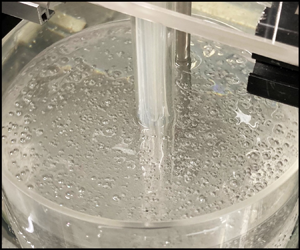
Here, the specifications of the bubble generation method in double concentric cylinders are explained. An acrylic plate was fixed to the inner cylinder, which was independent of the outer cylinder, as shown in figures 2(a) and 4(a). Four fine needles were mounted on the plate, and air was distributed by four pumps through silicone tubes located in the inner cylinder. Before starting the measurement in the oscillatory shear flow, the outer cylinder was rotated with a constant velocity of approximately  $6\ \mathrm {rpm}$, and fine bubbles with almost the same diameter (
 ${\leq }2\ \mathrm {mm}$) were generated in the silicone oil. Before starting the measurement, impellers were used to gently stir the suspension to evenly disperse the bubbles in the gap. The resulting volume fractions were
  $1.3\,\%$ and
  $1.1\,\%$ in 3000 and 5000 cSt silicon oil, respectively. Histograms of the bubble diameters are shown in figure 5. The De Brouchere average diameter, which is the ratio between the fourth and third moments of the size distribution, recently proposed by Mitrou et al. (Reference Mitrou, Migliozzi, Angeli and Mazzei2023), was used as the representative radius
  $a$ to calculate both the capillary and dynamic capillary numbers. The resulting diameters were
  $2a = 1.66$ and
  $1.15\ \mathrm {mm}$, as shown by the dashed lines in figure 5. These values correspond to the diameters at which the cumulative volume fractions were approximately
  $50\,\%$, as shown by the plus symbols in figure 5. Regarding spatial heterogeneity in the bubble volume fraction, it is considered to be negligible in both experiments. For the velocity-profiling-based rheometry, the spatial resolution of the ultrasonic transducer is a cylindrical shape with diameter of
  $10\ \mathrm {mm}$ and thickness of
  $O(1\ \mathrm {mm})$, more than a few bubbles are therefore included in the measurement volume. Furthermore, the viscoelasticity is not determined from the instantaneous velocity profile, but is analysed using the data from dozens of cycles, the velocity distribution of the bulk as the bubble suspension is captured by UVP measurement.

Figure 5. Histograms of the generated bubble diameters in (a) 3000 and (b)  $5000\ \mathrm {cSt}$ silicon oil. The dashed lines correspond to the De Brouchere average diameters, and the plus symbols indicate the cumulative volume fractions.


