


1. Introduction
The growth of vapour bubbles on heated solid surfaces under conditions of high superheating and low pressure is typically rapid. During this rapid expansion, which occurs shortly after the initial formation of a vapour bubble embryo, a thin micrometre-thick liquid layer is often trapped under the bubble on the solid surface (Moore & Mesler Reference Moore and Mesler1961; Tong & Tang Reference Tong and Tang2017), as depicted in the schematic in figure 1(a). Due to the microlayer's small thickness, heat conducted through it leads to rapid liquid evaporation. As a result, a high local heat transfer coefficient is achieved. Liquid evaporation from the microlayer is believed to make a significant contribution to the volume growth of the vapour bubble and to the high heat transfer performance observed in boiling phenomena (Cooper & Lloyd Reference Cooper and Lloyd1969; Chen et al. Reference Chen, Hu, Hu, Utaka and Mori2020; Bureš & Sato Reference Bureš and Sato2022; Tecchio et al. Reference Tecchio, Zhang, Cariteau, Zalczer, Roca i Cabarrocas, Bulkin, Charliac, Vassant and Nikolayev2022).

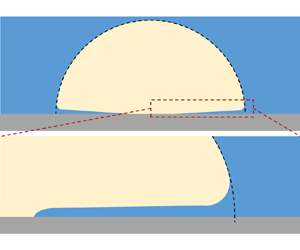
Figure 1. (a) A simplified illustration (not to scale) of a vapour bubble growing on a solid wall; the microlayer beneath the bubble is made thicker to aid visualisation. (b) Dragging of a viscous liquid by a moving plate, also known as the Landau–Levich problem.
The thickness of the microlayer, illustrated in figure 1(a), denotes the thickness of the portion of the liquid layer that is trapped under the bubble and away from the bubble front. Experimental observations (Jung & Kim Reference Jung and Kim2014; Sinha, Narayan & Srivastava Reference Sinha, Narayan and Srivastava2022; Tecchio et al. Reference Tecchio, Zhang, Cariteau, Zalczer, Roca i Cabarrocas, Bulkin, Charliac, Vassant and Nikolayev2022) have indicated that post-formation, the microlayer undergoes thinning due to evaporation, which depends on the initial thickness  $\delta _0$ when the microlayer is first created. The term ‘initial’ refers to the thickness of the microlayer when it is first deposited.
Several models have been proposed to determine the initial thickness of the microlayer. The boundary layer consideration has been a popular approach to determine this value used by researchers (Cooper & Lloyd Reference Cooper and Lloyd1969; Olander & Watts Reference Olander and Watts1969; van Ouwerkerk Reference van Ouwerkerk1971). As the bubble grows, it pushes the liquid outwards, leading to the development of a laminar boundary layer on the solid surface. The microlayer thickness  $\delta _0$ is assumed to be equal to the displacement thickness of this viscous boundary layer. A simple formula (1.1) was first derived by Cooper & Lloyd (Reference Cooper and Lloyd1969) based on the assumption that the bubble radius obeys an
  $R_b \propto t^{1/2}$ law:
 \begin{equation} \delta_0=C\sqrt{\nu t}, \end{equation}
where  $\nu$ is the liquid kinematic viscosity,
  $C$ is a constant, and
  $t$ is the growth time since nucleation. Equation (1.1) considers only the kinematic viscosity as a material parameter, and does not include the effect of surface tension, which was recently demonstrated to have an impact on the microlayer thickness (Hänsch & Walker Reference Hänsch and Walker2016).
The coefficient  $C$ has been subject to various estimations. Olander & Watts (Reference Olander and Watts1969) proposed
  $C=\sqrt {{\rm \pi} }/2$, while Cooper & Lloyd (Reference Cooper and Lloyd1969), accounting for short-lived effects of residual flows near the bubble front, suggested a slightly smaller value,
  $C\approx 0.8$. Details on the derivation of (1.1) and potential improvements of the underlying model are provided in Appendix A. van Ouwerkerk (Reference van Ouwerkerk1971) adopted a cylindrical geometry and proposed the coefficient
  $C\approx 1.27$. However, experimental measurements have indicated that this formula tends to overestimate the microlayer thickness. Empirical approaches using experimental data have also been employed to determine
  $C$, with reported values such as
  $C\approx 0.3\unicode{x2013}0.4$ for water (Koffman & Plesset Reference Koffman and Plesset1983), and
  $C\approx 0.22$ for ethanol vapour bubbles (Gao et al. Reference Gao, Zhang, Cheng and Quan2013).
Additionally, the predictions of (1.1) yield a monotonic increase in the thickness from the nucleation site, whilst recent experiments (Chen, Haginiwa & Utaka Reference Chen, Haginiwa and Utaka2017; Sinha et al. Reference Sinha, Narayan and Srivastava2022; Tecchio et al. Reference Tecchio, Zhang, Cariteau, Zalczer, Roca i Cabarrocas, Bulkin, Charliac, Vassant and Nikolayev2022) and computational fluid dynamics simulations (Hänsch & Walker Reference Hänsch and Walker2019) have revealed more complex liquid film profiles. A non-monotonic behaviour was observed, where the microlayer thickness initially increases, reaches a maximum and then decreases in its outermost part. This profile evolution was not explained by traditional boundary-layer approaches. The proportionality law of  $R_b\propto t^{0.5}$ was originally derived to describe the heat-transfer-controlled growth of bubbles in a uniformly superheated liquid (Plesset & Zwick Reference Plesset and Zwick1954; Mikic, Rohsenow & Griffith Reference Mikic, Rohsenow and Griffith1970). However, the validity of this law is questionable in practical situations where bubbles form upon heterogeneous nucleation on a heated wall and grow in a liquid with a non-uniform temperature.
A different approach was adopted by Smirnov (Reference Smirnov1975), who conducted a hydrodynamic analysis of the liquid flow near the bubble front and in the microlayer, assuming a two-dimensional axisymmetric radial flow. The formula that he proposed to calculate the microlayer thickness is
 \begin{equation} \delta_0=\sqrt{\frac{2\nu \dot{R}_b}{-9\ddot{R}_b-\dfrac{2R_b\dddot{R}_b}{\dot{R}_b}+\dfrac{2\dot{R}_b^2}{3R_b}}}, \end{equation}
where  $R_b$ is the bubble radius, and a dot over a quantity indicates its time derivative. Equation (1.2) does not depend on any specific bubble growth law. Upon a meticulous examination of the derivation, we identified flawed physical assumptions that raise concerns about the formula's validity. Detailed information is provided in Appendix B. Nevertheless, his approach has enlightening aspects, such as that the microlayer formation should be viewed as a local phenomenon linked to the liquid flow near the bubble front, rather than relating it to the liquid boundary layer outside the bubble as in the previous theories.
Katto & Shoji (Reference Katto and Shoji1970) argued that microlayer formation is intricately related to the flow of viscous liquid near the front of the bubble. This flow is driven by the pressure drop resulting from surface tension and changes in the curvature of the free interface. Zijl & Moalem-Maron (Reference Zijl and Moalem-Maron1978) were the first to hypothesise that the physical origin for microlayer formation is analogous to the thin liquid film deposited on a solid plate when it is withdrawn vertically from a liquid bath. This problem, famously known as the Landau–Levich film problem (Landau & Levich Reference Landau and Levich1942), offers useful insights into the microlayer formation mechanism.
Zijl & Moalem-Maron (Reference Zijl and Moalem-Maron1978) regarded the outward expanding bubble front as the meniscus formed in the Landau–Levich problem upon the free liquid surface, and estimated the microlayer thickness as
 \begin{equation} \delta_0=0.944\,\sqrt{2} \left( \frac{\mu u_m}{\sigma} \right)^{2/3} R_m, \end{equation}
with  $\mu$ being the liquid dynamic viscosity,
  $\sigma$ the surface tension,
  $u_m$ the speed of the bubble front, and
  $R_m$ the meniscus radius of curvature (see figure 1a). The latter was calculated via a modified expression of the capillary length where the meniscus acceleration replaced the gravitation acceleration:
 \begin{equation} R_m=\frac{1}{2} \left( -\frac{2\sigma}{\rho \ddot{R}_b} \right)^{1/2}, \end{equation}
where  $\rho$ is the liquid density. However, this line of thought was largely overlooked and did not gain popularity in microlayer studies.
Recently, Tecchio et al. (Reference Tecchio, Zhang, Cariteau, Zalczer, Roca i Cabarrocas, Bulkin, Charliac, Vassant and Nikolayev2022) revisited the Landau–Levich film to explain the outward-curved interface profile of the microlayer observed in their experiments. They hypothesised that the microlayer could be regarded as a liquid film deposited by the expansion of the bubble front. The decrease in the microlayer thickness was attributed to the reduction in the bubble expansion rate at the later growth stage. It was the first time a physical origin was provided for the non-monotonic profile, as the traditional boundary layer approach failed to do so. The value of  $R_m$ was determined from their experimental data. Kim & Seok Oh (Reference Kim and Seok Oh2021) also used (1.3) for predicting the initial microlayer thickness; however, they do not address the non-monotonic profile observed in experiments (Chen et al. Reference Chen, Haginiwa and Utaka2017; Utaka et al. Reference Utaka, Hu, Chen and Morokuma2018).
This study proposes a simple model for predicting the initial thickness of the microlayer. This prediction is grounded on a phenomenological comparison between the microlayer and the Landau–Levich film. The term ‘initial’ emphasises the pure hydrodynamic aspect of the problem, concentrating on the microlayer thickness immediately upon its formation. Therefore, microlayer thinning resulting from evaporation after its creation is not accounted for. For validation, we undertake a comparative study between the model predictions and experimental data, examining various bubble growth laws for both water and ethanol. A noteworthy feature of our model is that it is free from empirical constants. Subsequently, we use the model to address and explain contrasting experimental observations about the interface profile of the microlayer.
2. Problem formulation
We consider the axisymmetric growth of a vapour bubble on a flat smooth surface submerged in a large pool of liquid, as illustrated in figure 1(a). A two-dimensional axisymmetric reference frame  $(r, z)$ centred on the nucleation site is adopted, with
  $z$ indicating the vertical (axial) direction, and
  $r$ the horizontal (radial) direction. At a specific time moment
  $t_i$, the outer edge of the microlayer has reached the radial position
  $r_i$, located around the border of regions (II) and (III) in figure 1(a), with local thickness denoted as
  $\delta _0$. By collecting a series of
  $\delta _0$ values at different
  $r_i$ as time elapses, we can construct the initial thickness profile of the microlayer as a function of
  $r$, resulting in
  $\delta _0(r)$. The microlayer interface remains static once the microlayer is deposited on the solid without phase change or contact line motion (Zhang, El Mellas & Magnini Reference Zhang, El Mellas and Magnini2024). Hence the interface profile of the microlayer located on the left-hand side of the end of the microlayer (
 $r< r_i$) is the initial thickness of the microlayer,
  $\delta _0(r)$, depicted in figure 1(a), deposited before this instant
  $t_i$.
We investigate the rapid volumetric growth of the bubble. In reality, this phenomenon is observed in situations with high wall superheats, high wall heat fluxes, and low system pressures (Carey Reference Carey2020). The rapid growth pattern results in the bubble taking a nearly hemispherical shape, and also implies that a microlayer is likely trapped on the solid surface (Cooper & Lloyd Reference Cooper and Lloyd1969; Hänsch & Walker Reference Hänsch and Walker2016). We use  $R_b$ to denote the bubble's time-dependent hemispherical cap radius. The vapour in the bubble is at saturation with a uniform pressure
  $p_v$. The surrounding liquid is at a constant saturation state, characterised by a pressure
  $p_\infty$.
Our focus here is on the early stage of microlayer deposition by the expanding bubble, i.e. the hydrodynamic aspects of the microlayer. The phase change effect becomes apparent after the creation of the microlayer. Experimental observations have highlighted the thinning of the microlayer due to mass loss through evaporation, indicating that the microlayer creation is a faster process than evaporation. For instance, the microlayer is formed within  $1\,{\rm ms}$ for water at atmospheric pressure, whereas the time scales associated with the liquid evaporation are at least one order of magnitude larger (Utaka, Kashiwabara & Ozaki Reference Utaka, Kashiwabara and Ozaki2013; Chen et al. Reference Chen, Hu, Hu, Utaka and Mori2020). Therefore, it is possible to describe the microlayer formation from a pure hydrodynamic perspective.
The thickness of this microlayer is typically two to three orders of magnitude smaller than its radial extension,  $\delta /R_b \ll 1$; e.g. for water boiling at atmospheric pressure, the microlayer reaches thicknesses of a few micrometres, while its radial extension is of the order of 1 mm. Therefore, in this work, the evolution of this microlayer is described using the lubrication approximation. For
  $r \rightarrow 0$, the film terminates with a triple solid–liquid–vapour contact line, which leaves a dry patch centred at
  $r=0$. As
  $r \rightarrow \infty$, the microlayer profile joins the advancing bubble front at the bottom of the hemispherical cap of the bubble.
The microlayer can be divided into three distinct regions along the radial direction; see figure 1(a). The first (innermost) region is near the triple contact line. We consider a highly wettable solid surface to facilitate microlayer formation (Bureš & Sato Reference Bureš and Sato2021). The contact line receding is slow on wettable surfaces due to the small contact angle (Snoeijer & Eggers Reference Snoeijer and Eggers2010; Zhang & Nikolayev Reference Zhang and Nikolayev2022), thus its motion can be neglected during microlayer formation. After this phase, the expanding dry area may give rise to a dewetting ridge (Urbano et al. Reference Urbano, Tanguy, Huber and Colin2018; Tecchio et al. Reference Tecchio, Zhang, Cariteau, Zalczer, Roca i Cabarrocas, Bulkin, Charliac, Vassant and Nikolayev2022). However, this dewetting effect is out of the scope of this study. The second region is a thin layer of liquid, where the interface is nearly parallel to the solid surface, described in § 2.1 using the lubrication approximation. The third region is the bubble front, which takes a meniscus shape, described in § 2.2. The interface transitions from the nearly flat microlayer to the nearly hemispherical bubble dome of radius  $R_b$. We refer to the outermost part of the interface as the ‘bubble front’, identified by the radial position
  $r_f$, where
  $r_f$ also represents the width of the bubble, under the hemispherical assumption
  $r_f\approx R_b$. At the point of the interface transitioning between the last two regions, there exists a meniscus with the characteristic radius of curvature
  $R_m$ (Smirnov Reference Smirnov1975; Zijl & Moalem-Maron Reference Zijl and Moalem-Maron1978). This meniscus marks the outer edge of the microlayer and is responsible for determining the thickness of the deposited liquid film on the solid. We denote its outward-moving speed as
  $u_m$. The speed
  $u_m$ can be approximated as the bubble expansion rate
  $\dot {R}_b(t)$.
2.1. Equations for the thin film region
To emphasise the similarity of this problem with the Landau–Levich film (Landau & Levich Reference Landau and Levich1942), we change the axisymmetric coordinate system  $(r,z)$ to a planar coordinate system
  $(x,z)$, in a frame of reference moving with the bubble front
  $r_f$; see figure 1(b), where
  $x=-r+r_f$. The assumption of planar flow is justified by the slender nature of the microlayer with a thickness two orders of magnitude smaller than its radial extension
  $r$. In such a frame of reference, the solid wall is pulling up at speed
  $u_m$ with respect to the liquid bath, and a thin layer of liquid is deposited on it. Landau & Levich (Reference Landau and Levich1942) studied the problem of an infinite flat film. If the contact line is present, then when the film length is significantly larger than the thickness of the liquid film, Snoeijer et al. (Reference Snoeijer, Delon, Fermigier and Andreotti2006) has shown that the liquid film far from the contact line can still be described as the original Landau–Levich problem.
The original theory for determining the thickness of the liquid film was developed under the assumption of a solid moving at a constant speed, implying the static behaviour of the meniscus. The meniscus speed  $u_m$ generally decreases as the bubble grows larger, which does not satisfy static conditions. Nevertheless, Zhang & Nikolayev (Reference Zhang and Nikolayev2021) have demonstrated that the quasi-steady solution remains a valid approximation for dynamic scenarios in which the meniscus speed and curvature vary over time. It is shown that thin liquid films deposited on the inner walls of capillary tubes by receding menisci of liquid plugs remain nearly stationary after deposition due to high viscosity in the thin film if phase change is absent. A similar behaviour is expected for the microlayer. The initial thickness at a radial distance
  $r$ is determined by the speed
  $u_m$ and
  $R_m$ at the instant when the meniscus passes through
  $r$ (Zhang & Nikolayev Reference Zhang and Nikolayev2021).
For the thin film region in figure 1(b), Landau and Levich derived an equation describing the thickness  $\delta$ using the lubrication theory:
 \begin{equation} \frac{\partial^3\delta}{\partial x^3}=\frac{3\mu u_m}{\sigma}\,\frac{\delta_{0,LL}-\delta}{\delta^3}, \end{equation}
where  $\mu$ is the liquid viscosity, and
  $\sigma$ is surface tension. Unless otherwise indicated, all quantities used refer to the liquid phase. Here,
  $\delta _{0,LL}$ is the asymptotic liquid film thickness far from the meniscus region, where the interface tends to be parallel to the solid wall.
This is the upper boundary condition to (2.1):
 \begin{equation} \delta \to \delta_{0,LL}, \quad \frac{\partial \delta}{\partial x}\to 0 \quad \text{and} \quad \frac{\partial^2 \delta}{\partial x^2}\to 0, \quad \mbox{as}\ x \to \infty. \end{equation}
‘Upper’ refers to the relative direction indicated in figure 1(b). The lower boundary conditions are presented in § 2.3.
2.2. Equations for the meniscus region
In the meniscus region, across the curved interface, there is a discontinuity in normal stress that can be expressed by the Laplace equation
 \begin{equation} p(x)=p_v-\sigma K, \end{equation}
where  $p$ is the liquid pressure near the interface, and
  $K$ is the interface curvature calculated as the total curvature of a shell of revolution around the
  $z$-axis in figure 1(a) (Bucci Reference Bucci2020):
 \begin{equation} K=K_1+K_2 = \left[\frac{x}{\sin\left(\tan^{{-}1}\dfrac{\partial \delta}{\partial x}\right)}\right]^{{-}1} + \frac{\dfrac{\partial^2\delta}{\partial x^2}}{\left [ 1+\left( \dfrac{\partial \delta}{\partial x} \right)^2\right]^{3/2}}, \end{equation}
where  $K_1$ and
  $K_2$ are the parallel and meridian parts of the curvature, respectively. In the meniscus region, the interface slope is large, and
  $K_1$ satisfies
 \begin{equation} K_1 \approx \frac{1}{R_b}. \end{equation}
To obtain the liquid pressure near the interface in the third region, we use the full expression for the interface curvature in (2.4) and use the Rayleigh equation in the differential form (Tong & Tang Reference Tong and Tang2017),
 \begin{gather} \frac{\partial p}{\partial r}={-}\rho \left(\frac{2R_b\dot{R}_b^2+R_b^2\ddot{R}_b}{r^2} -\frac{2R_b^4\dot{R}_b^2}{r^5}\right), \end{gather}
 \begin{gather}\frac{\partial^2 p}{\partial r^2} = \rho \left(\frac{4 R_b \dot{R}_b^2+2 R_b^2\ddot{R}_b}{r^3} - \frac{10R_b^4\dot{R}_b^2}{r^6} \right), \end{gather}
where  $\rho$ is the density of the liquid. Equations (2.6) represent the liquid pressure gradient outside the interface of a growing bubble
  $R_b$ in a liquid of infinite extent. Constant liquid pressure
  $p_\infty$ is reached as
  $r\to \infty$.
Using (2.6), we approximate the liquid pressure near the interface as
 \begin{equation} p(r)\approx p(R_b) +(r-R_b) \left.\frac{\partial p}{\partial r}\right|_{r=R_b}+\frac{1}{2}\,(r-R_b)^2\left. \frac{\partial^2p}{\partial r^2}\right|_{r=R_b}. \end{equation}
Substituting the pressure derivatives using (2.6) results in
 \begin{equation} p(r)\approx p(R_b) - \rho \ddot{R}_b (r-R_b) - \rho\left[3\left(\frac{\dot{R}_b}{R_b}\right)^2 -\frac{\ddot{R}_b}{R_b}\right] (r-R_b)^2. \end{equation}
 Strictly speaking, (2.8) is applicable to the liquid outside the hemispherical interface. Regardless, we make the approximation of extending its application to the liquid area close to, but inside, the extension of the hemispherical interface (as depicted in the dashed region in figure 1(a)). This area is sufficiently distant from the solid surface, making boundary layer effects negligible. Taking (2.8) back to the frame of reference of the moving meniscus as in figure 1(b), and using  $x=-r+r_f$, leads to
 \begin{equation} p(x)\approx p(R_b) + \rho \ddot{R}_b x-\rho\left[3\left(\frac{\dot{R}_b}{R_b}\right)^2 -\frac{\ddot{R}_b}{R_b}\right]x^2, \end{equation}
where  $x$ is positive, representing the liquid pressure near the interface in the dashed area.
Incorporating the viscosity effect of bubble expansion and accounting for the usual discontinuity in normal stress, the pressure drop across the interface is given as (Tong & Tang Reference Tong and Tang2017)
 \begin{equation} p(R_b)=p_v-\frac{2\sigma}{R_b}-4\mu\,\frac{\dot{R}_b}{R_b}, \end{equation}
where the second and third terms on the right-hand side represent the contributions of surface tension and viscosity, respectively. To assess the relative importance of these two terms, we calculate the ratio of the viscous term to the surface tension term, and obtain  $2\mu \dot {R}_b/\sigma =2\,Ca_b\sim 10^{-2}$, where
  $Ca_b$ represents the capillary number of bubble growth. Since the ratio is small, the viscous effect on the pressure discontinuity across the interface will be omitted from further consideration.
Substituting (2.10) into (2.9) and then equating the obtained expression to (2.3), we find the equation for the dynamic meniscus in the transition region as
 \begin{equation} \frac{\dfrac{\partial^2\delta}{\partial x^2}}{\left [ 1+\left( \dfrac{\partial \delta}{\partial x} \right)^2\right]^{3/2}}=\frac{\rho}{\sigma}\left[3\left(\frac{\dot{R}_b}{R_b}\right)^2 -\frac{\ddot{R}_b}{R_b}\right]x^2 - \frac{\rho \ddot{R}_b}{\sigma}\,x + \frac{1}{R_b}. \end{equation}
 We integrate (2.11) in the interval  $[0,x]$, which produces
 \begin{equation} \frac{\dfrac{\partial \delta}{\partial x}}{\left [ 1+\left( \dfrac{\partial \delta}{\partial x} \right)^2\right]^{1/2}}=\frac{\rho}{\sigma}\left[\left(\frac{\dot{R}_b}{R_b}\right)^2 -\frac{\ddot{R}_b}{3R_b}\right]x^3 - \frac{\rho \ddot{R}_b}{2\sigma} x^2 + \frac{1}{R_b}\,x -1, \end{equation}
where the constant  $-1$ on the right-hand side is determined using the condition
  $\partial \delta /\partial x \to -\infty$ at
  $x\to 0$, i.e. the interface is nearly perpendicular to the solid surface. Equations (2.11) and (2.12) determine the thickness of the liquid
  $\delta$ in the meniscus region close to the bubble front.
2.3. Matching the thin film and meniscus regions
We first look at the meniscus region. At small values of  $\delta$, the solution of (2.11) and (2.12) must go over into the solution for the thin film region, which is governed by (2.1). Therefore, using the limit of small
  $\delta$, we have
  $\partial \delta /\partial x\to 0$ in the solution of the meniscus region. At the same time, the left-hand side of (2.12) approaches 0, and
  $x$ approaches a value denoted as
  $\bar {x}$. Its value is the positive root of the equation
 \begin{equation} a_3 x^3+a_2 x^2+a_1 x+a_0=0, \end{equation}
where
 \begin{equation} a_3 = \frac{\rho}{\sigma}\left[\left(\frac{\dot{R}_b}{R_b}\right)^2 -\frac{\ddot{R}_b}{3R_b}\right], \quad a_2 ={-} \frac{\rho \ddot{R}_b}{2\sigma}, \quad a_1=\frac{1}{R_b}, \quad a_0={-}1. \end{equation}
Note that  $\bar {x}=\sqrt {2\sigma /(\rho g)}$ is the characteristic length in the Landau–Levich original formulation (Landau & Levich Reference Landau and Levich1942).
The law of growth for  $R_b$ is commonly expressed as
  $R_b=C_b t^n$, where
  $C_b$ is a constant determined by the heating conditions and the properties of the liquid. For bubbles on solid surfaces during the thermal diffusion controlled stage, the value of
  $n$ is given theoretically as 0.5 by Mikic et al. (Reference Mikic, Rohsenow and Griffith1970), whilst in some experiments,
  $n<0.5$ is reported (Sinha et al. Reference Sinha, Narayan and Srivastava2022). The second time derivative
  $\ddot {R}_b=n(n-1)C_bt^{n-2}$ remains negative regardless. Consequently, the coefficients
  $a_3$,
  $a_2$ and
  $a_1$ are positive, and (2.13) possesses a single positive root.
With the help of (2.11), we find that the second derivative of  $\delta$ at
  $x=\bar {x}$ tends to
 \begin{equation} \left.\frac{\partial^2\delta}{\partial x^2} \right|_{x=\bar{x}}=3a_3 \bar{x}^2+2a_2\bar{x}+a_1, \end{equation}
which indicates that the meniscus region has a constant value of  $\partial ^2\delta /\partial x^2$ as the upper limit of the region.
The lower limit of the thin film region corresponds to the upper limit of the meniscus region, thus for matching the two solutions, we require the continuity of the second derivative  ${\partial ^2\delta }/{\partial x^2}$ as in Landau & Levich (Reference Landau and Levich1942). Equation (2.15) provides the sought lower boundary condition required for the solution of (2.1). Recall that the lubrication theory is applied to the thin film region, therefore the continuity of
  ${\partial ^2\delta }/{\partial x^2}$ indicates the continuity of the interface curvature as
  $\partial \delta /\partial x$ is small in this region. The constant identified at the right-hand side of (2.15) coincides with the curvature of the interface
  $1/R_m$, thus the lower boundary condition for (2.1) can be rewritten as
 \begin{equation} \left.\frac{\partial^2\delta}{\partial x^2} \right|_{\delta\to\infty}\to \frac{1}{R_m}, \end{equation}
where  $R_m$ is the radius of the characteristic curvature in the meniscus region, as illustrated in figure 1(a). Landau and Levich decided this matching point at
  $\bar {x}$, and the matching condition requires
 \begin{equation} \frac{1}{R_m}=\left.\frac{\partial^2\delta}{\partial x^2} \right|_{x=\bar{x}}. \end{equation}
Therefore, (2.16) and (2.17) provide the lower boundary conditions to (2.1). With the help of both upper and lower boundaries, a numerical solution to (2.1) has been given (Landau & Levich Reference Landau and Levich1942) as
 \begin{equation} \delta_0\approx1.34R_m\left(\frac{\mu u_m}{\sigma}\right)^{2/3}, \end{equation}
where the upper boundary condition  ${\delta _{0,LL}}$ is replaced with
  $\delta _0$ as we determine the initial microlayer thickness as a Landau–Levich film. In this equation,
  $R_m$ is calculated using (2.17) and (2.15), and
  $u_m$ can be equal to
  $\dot {R}_b$ approximately. The coefficient 1.34 in the equation was obtained numerically by Landau and Levich under the condition that
  $\mu u_m/\sigma$ is sufficiently small. This condition is generally satisfied as
  $\dot {R}_b\ll \sigma /\mu$ for a given fluid.
Equation (2.18) suggests that microlayer formation should result from a balance between surface tension, viscosity and inertial effects. While the above analysis applies the lubrication approximation and does not explicitly consider inertial effects, they play a significant role in the overall dynamics of bubble growth. The inertial effects impact the second time derivative of  $R_b$. This, in turn, influences the value of
  $R_m$ in the meniscus region. Our analysis maintains well-defined surface tension, with no shear stress applied to the interface. Factors like liquid impurities, surfactants and highly curved interfaces, which could lead to variations in interface temperature and non-uniform surface tension, are not taken into account.
Compared to the theory of determining the microlayer thickness as the displacement thickness of the hydrodynamic boundary layer outside the bubble on the solid (Cooper & Lloyd Reference Cooper and Lloyd1969; Olander & Watts Reference Olander and Watts1969), (2.18) incorporates the effect of surface tension and regards the formation of the microlayer as a local phenomenon due to the liquid flow near the bubble front. Notably, obtaining this equation is independent of the common assumption of the growth law as  $R_b\propto t^{0.5}$, which indicates that the equation can handle complex bubble growth patterns.
We must also notice that the derivation of (2.18) assumes the formation of the microlayer on smooth surfaces. In reality, given that  $\delta _0$ is typically of the order of a few micrometres, which can be close to the surface roughness, additional corrections may be necessary for surfaces with an absolute roughness of the order of
  $1\,\mathrm {\mu }{\rm m}$.
3. Validation and discussion
This section compares the prediction of (2.18) with experimental data on the initial microlayer thickness, and discusses some characteristics of the microlayer using the proposed model.
3.1. Experiments by Jung & Kim (Reference Jung and Kim2018)
Jung & Kim (Reference Jung and Kim2018) conducted experiments on single bubble nucleate boiling in a pool of saturated water under atmospheric pressure. The fluid properties of saturated water and steam (Harvey Reference Harvey1998) are summarised in table 1. Their experiment observed the growth of a bubble on an indium tin oxide (ITO) coated heater, driven by phase change. A high-speed camera captured the bubble growth, and  $R_b(t)$ was reported as plotted in figure 2. A microlayer was observed on the ITO surface, and its thickness was measured using laser interferometry. Due to the heat applied by the heater, liquid evaporated from the microlayer, resulting in a thinning of the microlayer. To account for this mass loss, they reconstructed the initial thickness of the microlayer
  $\delta _0(r)$ when it was initially deposited on the ITO surface, utilising the heater temperature data.

Figure 2. The Jung & Kim (Reference Jung and Kim2018) experimental data of bubble radius as a function of time (crosses), the power regression curve (solid line) and the bubble growth rate  $\dot {R}_b$ based on the regression curve (blue dashed line). The corresponding
  $R_m$ calculated by (2.17) is plotted in red.
Table 1. Fluid properties of saturated water  $(T_{sat}=373.15\,{{\rm K}})$ and ethanol
  $(T_{sat}=351.4\,{{\rm K}})$ at atmospheric pressure.

We established a power regression fitting curve for the Jung & Kim (Reference Jung and Kim2018) data for  $R_b(t)$ as
 \begin{equation} R_b(t)\approx0.0455t^{0.5}, \end{equation}
which provides the growth rate  $\dot {R}_b$ plotted in figure 2.
At each time instant, coefficients  $a_3$,
  $a_2$ and
  $a_1$ are calculated as indicated in (2.14), using known values of
  $\dot {R}_b$ and
  $\ddot {R}_b$. The value of
  $\bar {x}$ is then found by solving (2.13), and the corresponding
  $R_m$ is plotted in figure 2. When calculating
  $\delta _0$ using (2.18), we assume that the velocity of the bubble front is equal to the bubble growth rate:
  $u_m=\dot {R}_b$. For an adequate comparison, we also compute the predictions of (1.1) by Cooper & Lloyd (Reference Cooper and Lloyd1969) with
  $C=0.8$, (1.2) by Smirnov (Reference Smirnov1975), and (1.3) by Zijl & Moalem-Maron (Reference Zijl and Moalem-Maron1978).
Figure 3 presents a comparison of predictions for the initial microlayer thickness as a function of radial distance  $r$ based on (1.1), (1.2), (1.3) and (2.18). It is assumed that the thickness at a position
  $r$ is determined by the instant where the meniscus passes through. The initial thickness reconstructed from experimental measurements by Jung & Kim (Reference Jung and Kim2018) is also included in the plot for comparison. The microlayer thickness exhibits a consistent, monotonic increase from the nucleation site and remains below
  $6\,\mathrm {\mu }{\rm m}$ in the experimental data, which is in good agreement with the prediction of the proposed model (2.18). Despite the steady decrease in the bubble's growth rate, denoted as
  $\dot {R}_b$ or
  $u_m$, the radius of curvature
  $R_m$ continues to increase with
  $R_b$, surpassing the reduction in
  $\dot {R}_b$. This results in
  $\delta _0$, a product of
  $R_m$ and
  $u_m$, showing a rising trend. Notably, the predictions from (1.1) and (1.2) tend to overestimate the microlayer thickness by over
  $200\,\%$.

Figure 3. Initial thicknesses of the microlayer reconstructed from experimental data of Jung & Kim (Reference Jung and Kim2018) (circles), predicted by the proposed model of (2.18) (solid line), and from Cooper & Lloyd (Reference Cooper and Lloyd1969) (dash-dotted line), Smirnov (Reference Smirnov1975) (long dashed line) and Zijl & Moalem-Maron (Reference Zijl and Moalem-Maron1978) (short dashed line).
3.2. Experiments by Sinha et al. (Reference Sinha, Narayan and Srivastava2022)
Sinha et al. (Reference Sinha, Narayan and Srivastava2022) investigated bubble behaviour and microlayer dynamics during the growth of a single bubble on the heated solid wall of a vertical rectangular flow channel. The experiments were conducted with sub-cooled water under atmospheric pressure conditions. In the early rapid growth stage, both the bubble and microlayer exhibited symmetric expansion in the flow direction and perpendicular to the bulk flow, which led to the conclusion that the impact of bulk flow during the early stage was negligible, and the bubble growth process resembled that characteristic of pool boiling conditions. The thin-film interferometry technique, coupled with high-speed cinematography, captured the spatial and temporal evolution of the microlayer thickness. This approach allowed for recording the side view of the bubble as a function of time.
The experimentally recorded equivalent bubble radius  $R_b(t)$ for flow Reynolds number
  $Re=3600$ is represented by black crosses in figure 4. The growth law
  $R_b(t)\propto t^{0.5}$ is not suitable for accurately predicting the data in this experiment, as the bulk liquid is sub-cooled. The growth law
  $R_b(t)\propto t^{0.5}$ was originally developed for bubbles growing in a saturated liquid. Therefore, Sinha et al. (Reference Sinha, Narayan and Srivastava2022) used a power regression for the experimental data of
  $R_b(t)$,
 \begin{equation} R_b(t)\approx0.01652t^{0.4254}, \end{equation}
which is plotted as a black solid curve in figure 4. The bubble growth rate  $\dot {R}_b(t)$ and
  $R_m$ calculated by (2.17) are also obtained using the fitting curve of
  $R_b(t)$.

Figure 4. The Sinha et al. (Reference Sinha, Narayan and Srivastava2022) experimental data of bubble radius as a function of time (crosses), the power regression of (3.2) (solid line), and the bubble growth rate  $\dot {R}_b$ based on the regression curve (blue dashed line). The corresponding
  $R_m$ calculated by (2.17) is plotted in red.
Assuming  $u_m\approx \dot {R}_b(t)$, the predicted initial microlayer thickness
  $\delta _0$ from (2.18) is compared with the experimental data (circles) in figure 5. Equation (1.1) cannot provide a prediction as the growth law does not follow
  $R_b(t)\propto t^{0.5}$. Equations (1.2) and (1.3) can still be applied, and their predictions are shown as the long and short dashed lines in figure 5, respectively. Although the two equations are not limited by the assumption
  $R_b(t)\propto t^{0.5}$, they overestimate the thickness, especially (1.2), as the dashed lines are above the experimental data in figure 5. The proposed model generally yields thickness values that agree with the experimental measurement.

Figure 5. Initial thicknesses of the microlayer: experimental data of Sinha et al. (Reference Sinha, Narayan and Srivastava2022) (circles), and predictions by (2.18) (solid line), by Smirnov (Reference Smirnov1975) (long dashed line) and by Zijl & Moalem-Maron (Reference Zijl and Moalem-Maron1978) (short dashed line). The three rightmost data points are enlarged and shown in the inset.
A distinctive feature highlighted in the experiments of Sinha et al. (Reference Sinha, Narayan and Srivastava2022) is the reduction in microlayer thickness at its outer periphery, accompanied by a slight curvature in the interface. This characteristic is depicted in the inset of figure 5, where the rightmost data points are magnified for clarity. This non-monotonic behaviour is not captured by the proposed model, which predicts a constantly increasing thickness from the nucleation site. The non-monotonic aspect is addressed in § 3.3.2.
3.3. Some characteristics of the microlayer
3.3.1. Thickness dependence on the bubble growth rate
Chen et al. (Reference Chen, Hu, Hu, Utaka and Mori2020) conducted nucleate boiling experiments in a water pool under atmospheric pressure, measuring the microlayer thickness through laser interferometry across a wide range of heat fluxes, leading to various bubble growth rates. Their findings suggested a weak dependence of the initial microlayer thickness on the bubble expansion rate. This conclusion aligns with the earlier results obtained by Utaka et al. (Reference Utaka, Kashiwabara and Ozaki2013), who conducted similar experiments measuring the microlayer structure in nucleate pool boiling for water and ethanol under atmospheric pressure. Based on their experimental data, Utaka et al. (Reference Utaka, Kashiwabara and Ozaki2013) proposed two empirical formulas for predicting the initial microlayer thickness regardless of the growth rate:
 \begin{gather} \delta_0 (r) = 4.46\times10^{{-}3}r, \quad \text{water}, \end{gather}
 \begin{gather}\delta_0 (r) =1.02\times10^{{-}2}r, \quad \text{ethanol}, \end{gather}
where  $r$ is in mm, and
  $\delta _0$ is given in
  $\mathrm {\mu }{\rm m}$.
Yabuki & Nakabeppu (Reference Yabuki and Nakabeppu2014) also proposed an empirical formula based on their experiments of boiling bubbles on a heated surface in a pool of saturated water, as
 \begin{equation} \delta_0 (r) = 4.34 r^{0.69}, \end{equation}
where  $r$ is in millimetres, and
  $\delta _0$ is given in micrometres.
To test this feature of the microlayer, we employ the growth law proposed by Mikic et al. (Reference Mikic, Rohsenow and Griffith1970) for bubbles growing on a heated surface with temperature  $T_w$:
 \begin{equation} R_b(t)=C_b(\Delta T)t^{0.5}, \end{equation}
where  $C_b(\Delta T)=2\sqrt {{3}/{{\rm \pi} }}\,Ja\,\sqrt {\alpha }$ is the growth constant related to the solid superheat,
  $\Delta T= T_w - T_{sat}$,
  $T_{sat}$ is the saturation temperature of the liquid corresponding to the liquid pool pressure
  $p_\infty$, and
  $\alpha =k/(\rho c_p)$ is the thermal diffusivity. The Jakob number
  $Ja$ is defined as
 \begin{equation} Ja=\frac{\rho c_p (T_w - T_{sat})}{\rho_v \mathcal{L}}, \end{equation}
where  $c_p$ is the heat capacity of the liquid,
  $\rho _v$ is the density of the vapour, and
  $\mathcal {L}$ is the latent heat. Various bubble growth rates are achieved by tuning
  $\Delta T$.
Equation (3.5) is employed to describe the bubble growth during the diffusion-controlled stage on superheated solid surfaces in a uniformly saturated liquid. We disregard the initial inertia-controlled growth, typically occurring within a duration shorter than  $0.1\,{\rm ms}$ (Mikic et al. Reference Mikic, Rohsenow and Griffith1970). Two distinct superheat conditions are considered, with
  $\Delta T = 10\,{{\rm K}}$ and
  $25\,{\rm K}$, assuming that the bubble growth on the solid surface adheres to (3.5) and that its interface is nearly hemispherical, implying
  $u_m \approx \dot {R}_b$. The microlayer thickness
  $\delta _0$, predicted by (2.18), is computed and plotted against the radial distance from the nucleate site
  $r$ in figure 6. The experimentally obtained (3.3) and (3.4) are presented in the same plot. The fluid properties of saturated water and ethanol at atmospheric pressure are listed in table 1.

Figure 6. Comparison of the initial microlayer thickness predicted by the present model and empirical formulas of Utaka et al. (Reference Utaka, Kashiwabara and Ozaki2013) and Yabuki & Nakabeppu (Reference Yabuki and Nakabeppu2014): (a) water, (b) ethanol.
The prediction of the initial microlayer thickness by the present model is in good agreement with the empirical relations (3.3) and (3.4). The variation in microlayer thickness exhibits weak dependence on the change in the superheat conditions. For water, the growth rates are  $C_b(10\,{\rm K}) \approx 2.4\times 10^{-2} \,{\rm m}\,{\rm s}^{-0.5}$ and
  $C_b(25\,{\rm K}) \approx 6.0\times 10^{-2} \,{\rm m}\,{\rm s}^{-0.5}$. For ethanol, the growth rates are
  $C_b(10\,{\rm K}) \approx 8.4\times 10^{-3} \,{\rm m}\,{\rm s}^{-0.5}$ and
  $C_b(25\,{\rm K}) \approx 2.1\times 10^{-2} \,{\rm m}\,{\rm s}^{-0.5}$. Despite a 2.5-fold alteration in the growth rate, the corresponding change in
  $\delta _0$ is less than 20 %. This observation aligns with experimental findings, confirming that the initial microlayer thickness demonstrates little sensitivity to heat flux, i.e. to the bubble expansion rate (Utaka et al. Reference Utaka, Kashiwabara and Ozaki2013; Chen et al. Reference Chen, Hu, Hu, Utaka and Mori2020). The present model also predicts that the microlayer thickness of ethanol is about 1.5 larger than that of water at the same
  $r$. This is also in agreement with experimental observations (Koffman & Plesset Reference Koffman and Plesset1983).
3.3.2. Spatial variation of the interface profile
In the preceding subsection, we used the assumption of  $R_b(t)\propto t^{0.5}$, a common feature in multiple theories that predict the microlayer thickness. The resultant spatial profile of the microlayer exhibits a steady increase from the nucleation site. This wedge-like microlayer structure aligns with observations from many experiments (Utaka et al. Reference Utaka, Kashiwabara and Ozaki2013; Jung & Kim Reference Jung and Kim2014, Reference Jung and Kim2018; Chen et al. Reference Chen, Hu, Hu, Utaka and Mori2020).
A non-monotonic profile of microlayer thickness has also been reported: it reaches a plateau in the middle, then decreases towards the outer edge of the meniscus, resembling an interface bent like a speed bump with a local maximal thickness (Chen et al. Reference Chen, Haginiwa and Utaka2017; Sinha et al. Reference Sinha, Narayan and Srivastava2022; Tecchio et al. Reference Tecchio, Zhang, Cariteau, Zalczer, Roca i Cabarrocas, Bulkin, Charliac, Vassant and Nikolayev2022). This distinctive pattern mirrors the film deposited by a meniscus travelling at non-constant speeds in capillary tubes, a phenomenon observed experimentally by Youn et al. (Reference Youn, Muramatsu, Han and Shikazono2016) and Youn, Han & Shikazono (Reference Youn, Han and Shikazono2018), and explained theoretically by Zhang & Nikolayev (Reference Zhang and Nikolayev2021) using the Landau–Levich film problem under unsteady conditions. As depicted in (2.18), the thickness results from the product of the radius of curvature of the meniscus and its advancing speed. Throughout the entire process of a bubble growing on solid surfaces, the bubble undergoes expansion at a decelerating rate:  $R_b$ increases monotonically with time, yet
  $\ddot {R}_b$ is negative. In the later stages of bubble growth, the microlayer's width nearly halts expansion on the solid, and the expansion speed approaches zero. Consequently, the resulting thickness calculated by (2.18) could decrease, suggesting the possibility of a maximal thickness during the process.
Moreover, in real-world scenarios, the values of  $R_b(t)$ and the bubble's width on the solid should eventually approach a maximal value, in contrast to the implication of the proportionality law
  $R_b(t)\propto t^n$, which suggests an indefinite growth of
  $R_b(t)$. This highlights the need for a more nuanced model that accounts for the eventual stabilisation of these parameters at later stages. To address this, we propose a function
 \begin{equation} R_b(t) = R_c - (R_c - C_b t^n)\,{\rm e}^{{-}t/t_c}, \end{equation}
where  $R_c$ represents the radius towards which the bubble approaches the end stage of growth, and
  $t_c$ characterises the rate at which the bubble approaches
  $R_c$. For small
  $t$, this function approximates
  $R_b(t)\approx C_b t^n$, implying adherence to the power growth law that can be determined as in (3.5). As
  $t$ approaches
  $t_c$,
  $R_b(t)\approx R_c$, indicating that the bubble is close to a non-growth stage. This construction more accurately reflects real-world situations, providing a more realistic representation of bubble growth dynamics.
The experimental data of  $R_b(t)$ by Sinha et al. (Reference Sinha, Narayan and Srivastava2022) are employed to determine the parameters in (3.7). The regression curve is depicted in figure 7, with
  $R_c=1.10\times 10^{-3}\,{\rm m}$,
  $C_b=2.58\times 10^{-2}\,{\rm m}\,{\rm s}^{-0.5}$,
  $n=0.5$ and
  $t_c=1.96\times 10^{-3}\,{\rm s}$. Compared with the regression curve for
  $R_b$ in figure 4, (3.7) aligns more closely with the experimental data, particularly for larger
  $t$. Using the new regression curve, (2.18) is employed to compute the microlayer thickness as a function of
  $r$. The results are plotted and compared in figure 8. The slight change in the behaviour of
  $R_b$ results in a noticeable alteration in the microlayer profile: the thickness no longer exhibits a monotonic increase, but instead features a maximal value before decreasing. The resulting profile shows an outward curvature, resembling the observations made by Sinha et al. (Reference Sinha, Narayan and Srivastava2022).

Figure 7. The Sinha et al. (Reference Sinha, Narayan and Srivastava2022) experimental data of bubble radius as a function of time (crosses), the regression of (3.7) (solid line), and the bubble growth rate  $\dot {R}_b$ based on the regression curve (blue dashed line). The corresponding
  $R_m$ calculated by (2.17) is plotted in red.

Figure 8. Initial thicknesses of the microlayer: experimental data of Sinha et al. (Reference Sinha, Narayan and Srivastava2022) (circles), and prediction by (2.18) (solid line) using (3.7) to describe the bubble growth rate.
We consider another simplified scenario to highlight the expansion deceleration effect on the microlayer profile. We construct two laws of growth using (3.5) and (3.7), setting  $C_b=3\times 10^{-2}\,{\rm m}\,{\rm s}^{-0.5}$ in both equations. We introduce a minor deceleration effect by setting
  $R_c=9.5\times 10^{-4}\,{\rm m}$ and
  $t_c=3\times 10^{-3}\,{\rm s}$ in (3.7). Consequently, for small
  $t$, the bubble growth of both equations closely follows the power law, while for larger
  $t$, the growth decelerates as specified in (3.7), where
  $R_b$ approaches
  $R_c$. The respective bubble radii as functions of time, specified by the two growth laws, are illustrated in figure 9. The corresponding bubble growth rates
  $\dot {R}_b$ and
  $R_m$, calculated using (2.17), are also depicted. As expected,
  $\dot {R}_b$ exhibits a lower rate for the growth law of (3.7) when
  $t$ is large. By applying these growth laws, we can calculate the initial thickness of the microlayer as predicted by the model. The results are presented in figure 10. At small
  $r$ (i.e. short
  $t$), the microlayer thicknesses are comparable. However, for larger
  $r$, the microlayer thickness for the bubble growth specified by the unstopped growth law of (3.5) continues to increase, while the growth governed by (3.7) reaches a plateau before decreasing. This behaviour illustrates a bent overall interface profile. It is noteworthy that although the two growth laws for
  $R_b$ in figure 9 almost overlap, with their difference likely being comparable to the experimental uncertainty in the bubble volume measurement, the resulting microlayer thicknesses may differ by up to 30 % at its outer periphery (
 $r=1\,\mathrm {mm}$).

Figure 9. Comparison of the two laws of growth for the bubble radius  $R_b$: unstopped as specified by (3.5) (dashed lines) and subsiding as calculated by (3.7) (solid lines). The bubble growth rates
  $\dot {R}_b$ are plotted in blue, and the corresponding
  $R_m$ calculated by (2.17) are plotted in red.

The objective of comparing the two growth laws is to attribute the curved interface profile of the microlayer to the deceleration effect in the expansion rate of the microlayer's outer edge, which is assumed to be equal to the bubble's expansion rate on the solid in the current formulation. Under idealised conditions where the bulk liquid is perfectly superheated, the bubble radius on the solid as a function of time may indeed follow the power law described by (3.5) for an extended period of time. Consequently, the initial thickness of the microlayer would exhibit continuous, non-stop growth from the nucleation site. This scenario might be the case presented in § 3.1, where  $R_b(t)$ was well-fitted by (3.5) in figure 2, and a wedge-like profile was observed. The deceleration effect becomes more pronounced when the bulk liquid is sub-cooled or only at saturation. In such cases, the bubble can maintain a fast growth rate at an early stage while it stays in the superheated thermal boundary layer on the solid surface. As the bubble grows taller, it protrudes out of the thermal boundary layer and comes into contact with the sub-cooled liquid; a significant reduction in the growth rate occurs, as the heat transfer from the interface becomes insufficient to sustain the earlier growth rate. The thermal boundary thickness
  $\delta _t$ on a heated wall in a liquid pool can be calculated as (Kays, Crawford & Weigand Reference Kays, Crawford and Weigand2004)
 \begin{equation} \delta_t \approx 7.14 \left(\frac{\mu \alpha}{\rho g \beta\,\Delta T} \right)^{1/3}, \end{equation}
where  $\beta$ is the thermal expansion coefficient of the liquid, and
  $g$ is the gravitational acceleration. For water on a solid wall superheated by
  $10\,{\rm K}$,
  $\delta _t\approx 0.62\,{\rm mm}$, which can be smaller than the bubble radius.
Another factor affecting the bubble's expansion on the solid surface is buoyancy, which tends to lift the bubble away from the surface. This effect becomes more pronounced as the bubble grows larger and contributes to the deviation of the bubble from a hemispherical shape (Zhang et al. Reference Zhang, El Mellas and Magnini2024).
We must underline that we refrain from asserting that (3.7) is the definitive or exclusive function to describe the behaviour of  $R_b(t)$. Instead, we emphasise that (3.7) serves as one possible simple expression that accounts for the observed slowing-down effect in the radius of vapour bubbles during the later stages of growth on heated solid surfaces. This phenomenon is commonly encountered in practice, contrasting with the idealised proportionality law
  $R_b(t)\propto t^n$, which implies non-stop bubble expansion.
Another noteworthy observation pertains to the situation when the meniscus reaches its maximum width, at which  $u_m$ approaches 0. According to the prediction from (2.18), the thickness then becomes 0. This would impact only a small portion of the thickness prediction. A comparable phenomenon is observed in the meniscus oscillation in capillary tubes. When the meniscus speed decelerates to zero during the deposition of a liquid film, the film thickness decreases but does not reach zero when the meniscus speed decreases to zero (Youn et al. Reference Youn, Han and Shikazono2018; Zhang & Nikolayev Reference Zhang and Nikolayev2021). The liquid film remains attached to the meniscus, and so does the microlayer.
4. Conclusions
We propose a phenomenological model that estimates the initial thickness of the microlayer forming under vapour bubbles growing on solid surfaces. This model conceptualises the microlayer as analogous to the liquid film in the Landau–Levich problem. In this framework, the microlayer formation is governed by the liquid flow near the bubble front of the bubble on the solid, and its thickness is determined by the balance of surface tension and viscous forces. Our model offers a broader range of applications, unlike the previous theories relying on specific bubble growth laws as  $R_b(t)\propto t^{0.5}$.
We employ the model to compute microlayer thickness under water and ethanol bubbles growing under varying conditions. The comparisons with experimental data have shown good agreement. Considering the idealised growth law for bubbles  $R_b(t)=C_b t^{0.5}$, the model predicts that microlayer thickness is insensitive to the growth coefficient
  $C_b$, which is associated with the solid's heating flux or, more broadly, the heating conditions of the solid. This observation agrees with previous experimental findings, where the microlayer under water vapour bubbles typically measures below
  $5\,\mathrm {\mu }{\rm m}$ at extension 1 mm from the nucleation site, regardless of the heating conditions.
Later, we use the model to investigate the interface profile of the microlayer, addressing inconsistent reports in previous studies. Some reported a wedge-like microlayer with thickness steadily increasing from the nucleation site. Others reported a slightly outwardly curved profile, reaching maximal thickness in the middle, and tapering towards the outermost part of the microlayer. We attribute the decrease in microlayer thickness to the slowing down of the microlayer expansion rate. This is often linked to the deceleration of the bubble growth rate as the bubble reaches its maximum width on the solid surface. In situations where the microlayer can expand on the solid with the bubble unconstrained, the microlayer thickness will continue to increase constantly. In real-world situations where the bubble experiences a significant reduction in growth rate near its maximal width, the microlayer thickness decreases accordingly. This explains the observed thinner microlayer near the outermost part when the growth slows down compared to earlier stages.
Knowledge of microlayer features from the model can contribute to developing mechanistic models for nucleate boiling heat transfer. Those models require accurate information on the microlayer thickness and growth behaviour as the evaporative heat flux through the microlayer is believed to influence total boiling heat transfer significantly.
Acknowledgements
The authors express gratitude to Dr V. Nikolayev, Director of Research at the French Alternative Energies and Atomic Energy Commission (CEA), Paris-Saclay Centre, for valuable and constructive discussions on the paper.
Funding
This work is supported by the UK Engineering & Physical Sciences Research Council (EPSRC), through the BONSAI (EP/T033398/1) grant.
Declaration of interests
The authors report no conflict of interest.
Appendix A. Comments on Cooper & Lloyd (Reference Cooper and Lloyd1969)
Cooper & Lloyd (Reference Cooper and Lloyd1969) proposed a simplified hydrodynamic theory that predicts the initial thickness of the microlayer as the displacement thickness of the boundary layer outside a growing bubble. The flow is assumed to be two-dimensional.
The flow pattern in region A (well outside the bubble) is sketched in figure 11(a). The liquid velocity reduces from a uniform outward radial velocity to zero in a boundary layer near the wall. The liquid in the microlayer near the bubble front (region C) is not stationary, whilst the velocity decays rapidly in a time of the order of  $\delta ^2/4\nu$. In region D, the liquid away from the bubble front can be considered at rest.

Figure 11. (a) Sketch of a growing bubble on the solid and liquid flow. (b) Liquid flow pattern in the frame of reference of the moving wall, where the latter moves at a speed  $u_w$ towards the left.
Obtaining an analytical flow pattern in region B is difficult, as inertial, viscous and surface tension forces are all significant. Cooper & Lloyd (Reference Cooper and Lloyd1969) applied a velocity  $-u_b$ in the
  $r$-direction to the flow in figure 11(a), which gives the flow pattern sketched in figure 11(b) when observed from a reference frame moving with the bubble front: the free interface is nearly stationary, and the liquid velocity
  $u'(z,t)=u-u_b$ is parallel to the wall. The mass conservation is the major assumption in the original paper, which states that liquid flow from the right-hand side is equal to the rate flowing out at the left-hand side:
 \begin{align} \delta_0 u_b=\int_0^\infty u'\,{\rm d}z, \end{align}
where the microlayer thickness  $\delta _0$ can be regarded as the displacement thickness of the boundary layer in Stokes’ first problem, which determines the flow created by a sudden movement of an infinitely long plate to speed
  $u_w$ from rest. The Navier–Stokes equation for such a problem is reduced to
 \begin{align} \frac{\partial u'}{\partial t}=\nu\,\frac{\partial^2 u'}{\partial z^2} \end{align}
with boundary conditions
 \begin{gather} u'(z)=0 \quad \text{when} \ t=0, \end{gather}
 \begin{gather}u'(0)=u_w(r,t) \quad \text{and} \quad u'(\infty)=0 \quad \text{when} \ t>0, \end{gather}
where the velocity  $u_w(r,t)$ of the wall is defined below. When solving (A2), Cooper & Lloyd (Reference Cooper and Lloyd1969) used
 \begin{equation} u_w(r,t)=\frac{\dot{V}}{2{\rm \pi} r^2}=C'(r)\,t^n, \end{equation}
where the bubble volume growth rate was estimated as  $\dot {V}=2{\rm \pi} C_b^3nt^{3n-1}$, with the bubble radius calculated as
  $R_b(t)=C_b t^n$. They took
  $n=0.5$ and applied
  $u_w(r,t)=C'(r)t^{0.5}$ to (A3b). A simple form of
  $u'$ can then be obtained as
 \begin{equation} u'=u_w\,\sqrt{\rm \pi} \text{ierfc}\left(\frac{z}{2\sqrt{\nu t}}\right), \end{equation}
where  $\text {ierfc}(x)$ is the integral of the complementary error function
  $\text {ierfc}(\xi )$ from
  $x$ to
  $\infty$. Therefore,
 \begin{equation} \int_0^\infty u'\,{\rm d}z=u_w\,\frac{\sqrt{\rm \pi}}{2}\,\sqrt{\nu t}. \end{equation}
 In substituting (A6) into (A1), Cooper & Lloyd (Reference Cooper and Lloyd1969) argued that  $u_w=u_b$, and consequently obtained
 \begin{equation} \delta_0=\frac{\sqrt{\rm \pi}}{2}\,\sqrt{\nu t}. \end{equation}
However, under the hemispherical bubble approximation,  $u_b(t)$ should equal
  $\dot {R}_{b}=0.5C_b t^{-0.5}$, which is inconsistent with their assumption
  $u_w\propto t^{0.5}$ made in the boundary condition (A3b).
As a matter of fact,  $u_w$ should have the form
 \begin{equation} u_w(r,t)=\frac{R_b^2}{r^2}\,u_b(t) \end{equation}
where  $r>R_b$, and when the bubble passes the point in question
  $r=R_b$, we have
  $u_w=u_b$.
Applying (A8) to boundary condition (A3b), we obtain (Carslaw & Jaeger Reference Carslaw and Jaeger1959)
 \begin{equation} u'=\frac{z}{2\sqrt{{\rm \pi} \nu}}\int_0^t \frac{u_b(\tau)}{(t-\tau)^{3/2}}\exp\left({\frac{-z^2}{4\nu(t-\tau)}}\right) \,{\rm d}\tau. \end{equation}
 The displacement thickness or the microlayer thickness is then calculated by integrating  $u'$ from
  $z=0$ to infinity using (A1). Equating the microlayer thickness to the displacement thickness of the viscous boundary layer can be considered reasonable when liquid dynamics in the meniscus region is governed primarily by inertial effects. To estimate the importance of inertia, one can calculate the Bond number (
 $Bo$) based on the interface acceleration:
 \begin{equation} Bo = \frac{\Delta \rho\,L^2\,|a_b|}{\sigma}, \end{equation}
where  $\Delta \rho$ is the difference in density between the two phases,
  $L$ is the characteristic length of the meniscus (of the order of 0.1 mm), and
  $a_b$ is the acceleration of the bubble interface. The Bond number is smaller than 1 in the meniscus region, which indicates that the surface tension effect should not be neglected, and using the displacement thickness would lead to an overestimation of the microlayer thickness.
Appendix B. Review of Smirnov (Reference Smirnov1975)
Smirnov performed a hydrodynamic analysis of the microlayer in the two-dimensional axisymmetric cylindrical coordinates with simplifications from the lubrication theory. After a meticulous re-examination of his paper, we have found that his formulation contains flawed physical assumptions and derivations. We believe that it is important to show these mistakes as Smirnov's theory is popular in microlayer description.
B.1. Governing equations
In the lubrication theory, the liquid in the microlayer moves primarily in the  $r$-direction, implying
  $u_z \ll u_r$. The equation of momentum in two-dimensional axisymmetric cylindrical coordinates was written as
 \begin{equation} \frac{\partial u_r}{\partial t} + u_r\,\frac{\partial u_r}{\partial r} ={-}\frac{1}{\rho}\,\frac{\partial p}{\partial r}+\nu \left(\nabla^2u_r- \frac{u_r}{r^2} \right), \end{equation}
where
 \begin{equation} \nabla^2u_r = \frac{1}{r}\,\frac{\partial u_r}{\partial r} + \frac{\partial^2 u_r}{\partial r^2} + \frac{\partial^2 u_r}{\partial z^2}. \end{equation}
The equation of continuity in the original paper was written as
 \begin{equation} \frac{\partial}{\partial r}\left(ru_r\delta_0\right)=0, \end{equation}
where  $u_r(r, z)$ is the liquid velocity in the
  $r$-direction, and
  $\delta _0$ is the initial thickness of the microlayer.
Without considering phase change, and assuming that the interface stands still once created, the correct form of the continuity equation in the microlayer should be written as (Zhang & Nikolayev Reference Zhang and Nikolayev2021)
 \begin{equation} \frac{\partial \varPhi(r)}{\partial r}=0, \end{equation}
where  $\varPhi (r)$ represents the liquid volumetric flux through the lateral surface of the cylinder in the microlayer at
  $r$, which can be expressed as
 \begin{equation} \varPhi(r)=2{\rm \pi} r \int_0^{\delta_0}u_r \,{\rm d}z. \end{equation}
The equation of continuity should then be written as
 \begin{equation} \frac{\partial}{\partial r}\left( r\int_0^{\delta_0}u_r \,{\rm d}z \right) = 0. \end{equation}
B.2. Boundary conditions
Smirnov introduced an assumption regarding the profile of  $u_r(z)$ at
  $r=R_b$ by assuming it as a separation of variables, expressed as
 \begin{equation} u_r=\dot{R}_b\,\frac{z}{\delta_0}\,f_2(t), \end{equation}
where  $f_2(t)$ is a function of time, with
  $t=0$ corresponding to the moment where the microlayer is created. At a given position
  $r$, when the bubble interface passes through,
  $t=0$ and
  $f_2(0)=1$. The value of
  $f_2(t)$ should decay rapidly as the microlayer does not vary with time if evaporation is absent.
Equation (B7) implies a linear variation of  $u_r(z)$ from the solid surface to the interface for a given moment
  $t>0$. However, this assumption leads to a non-zero velocity gradient at the free interface:
  ${\partial u_r}/{\partial z} \neq 0$ at
  $z = \delta _0$, indicating the presence of shear stress on the interface. In practice, this assumption does not hold true for liquid–vapour interfaces if the surface tension is assumed constant, where shear stress at the interface is typically non-existent.
Take a step back. Even if we concede that (B7) is reasonable, one substitutes (B7) into (B6) and the equation of continuity becomes
 \begin{equation} \frac{\partial}{\partial r}\left(r \dot{R}_b \delta_0 \right)=0, \end{equation}
which is inconsistent with the original equation of continuity (B3).
Later, Smirnov used (B3) to obtain
 \begin{equation} \frac{\partial u_r}{\partial r} ={-} \frac{u_r}{r}- \frac{u_r}{\delta_0}\,\frac{\partial \delta_0}{\partial r} \end{equation}
and
 \begin{equation} \frac{\partial^2 u_r}{\partial r^2} =\frac{2 u_r}{r^2} + \frac{2u_r}{r\delta_0}\,\frac{\partial \delta_0}{\partial r} + \frac{2u_r}{\delta_0^2} \left(\frac{\partial \delta_0}{\partial r} \right)^2- \frac{u_r}{\delta_0}\,\frac{\partial^2 \delta_0}{\partial r^2}. \end{equation}
 Smirnov argued that one should examine the equation of momentum only when the microlayer is just created, where  $t=0$, and assumed
  $\partial r=\partial R_b$. Substituting (B7) into (B1) using (B9) and (B10), then integrating the obtained expression from
  $z=0$ to
  $z=\delta _0$, one arrives at equation (8) of Smirnov (Reference Smirnov1975). The coefficient of the second term on the left-hand side of equation (8) should be
  $-2/3$, instead of
  $-2$ as stated in the original paper.
During the processing, the integration of  ${\partial ^2 u_r}/{\partial z^2}$ on the right-hand side was performed by Smirnov as
 \begin{equation} \int_0^{\delta_0} \frac{\partial^2 u_r}{\partial z^2} \,{\rm d}z= \left. \frac{\partial u_r} {\partial z} \right |_{z=\delta_0}- \left. \frac{\partial u_r} {\partial z} \right |_{z=0}= 0- \frac{\dot{R}_b}{\delta_0}, \end{equation}
which is inconsistent with the assumed velocity profile (B7).
After the integration, the calculating equation for determining the initial thickness was then expressed as
 \begin{equation} \delta_0 =\sqrt{\frac{2 \nu \dot{R}_b}{-\dfrac{2}{\rho}\,\dfrac{\partial p}{\partial R_b} -\ddot{R}_b + \dfrac{2 \dot{R}_b^2}{3 R_b} }}, \end{equation}
where  $p$ is the pressure in the liquid at the phase interface. It can be calculated using the Rayleigh equation
 \begin{equation} \frac{p-p_\infty}{\rho} = R_b \ddot{R}_b + \frac{3}{2}\,\dot{R}_b^2. \end{equation}
 In equation (11) of the original paper, an additional term  ${2\sigma }/{\rho R_b}$ was introduced on the right-hand side of (B13) to account for the discontinuity of the normal stress across the phase interface. However, given that
  $p$ represents the pressure in the liquid, there seems to be no appropriate place for introducing this discontinuity in (B13). This suggests that the surface tension effect should not have been included in the theory in the first place.
B.3. Liquid pressure gradient
To obtain the gradient of the liquid pressure  ${\partial p}/{\partial R_b}$, Smirnov took the time derivative on both sides of (B13) and made the assumption
 \begin{equation} \left. \frac{\partial p}{\partial r} \right |_{r=R_b} =\frac{\partial p}{\partial t} \, \frac{\partial t} {\partial R_b}. \end{equation}
Estimating the liquid pressure gradient using the substitution of (B14) raises questions about the validity of the approach, a concern that has also been raised by Bureš & Sato (Reference Bureš and Sato2022).
Recently, Jung & Kim (Reference Jung and Kim2018) reintroduced the surface tension effect, which should not have been included, as demonstrated above. Nonetheless, a mistake exists in their formulation. The last term in the denominator of equation (11) in Jung & Kim (Reference Jung and Kim2018) is incorrectly expressed as this term must be dimensionless, and as such, it should be represented as
 \begin{equation} \delta_0=\sqrt{\frac{2\nu t}{9(1-n)+2\left(\dfrac{1}{n}-1\right)(n-2)+0.66n+\dfrac{4\sigma}{\rho C_b^3nt^{3n-2}}}}, \end{equation}
where the bubble takes the law of growth in the form  $R_b=C_b t^n$. This error also appears in Sinha et al. (Reference Sinha, Narayan and Srivastava2022), which used the Jung & Kim (Reference Jung and Kim2018) formula. One can estimate the surface tension correction, the last term of the denominator on the right-hand side of (B15), by assuming
  $n=0.5$ and
  $C_b = 3\times 10^{-2} \,{\rm m}\,{\rm s}^{-0.5}$. This term is then calculated for water using fluid properties in table 1:
 \begin{equation} \frac{4\sigma}{\rho C_b^3nt^{3n-2}} \approx 0.0242t^{0.5}. \end{equation}
For  $t=1\,{\rm ms}$, this term gives a correction of approximately
  $7.65\times 10^{-4}$, which is much smaller than the sum of the rest in the denominator of 2.33 in (B15).
Since the original equation by Smirnov (Reference Smirnov1975) contains flawed physical assumptions, utilising an equation based on the original one may lead to results that lack physical coherence.


 Open access