


1. Introduction
Randomly distributed particles can spontaneously migrate across streamlines in channel flows and eventually focus at specific regions or locations within the cross-section. In the pioneering experimental work of Segré & Silberberg (Reference Segré and Silberberg1961), particles migrate across streamlines and focus into a ring in a circular pipe. Since then, experimental studies have extensively investigated particle focusing in straight channels by varying the channel Reynolds number, the shape of the channel cross-section and the particle size (Matas, Morris & Guazzelli Reference Matas, Morris and Guazzelli2004; Di Carlo et al. Reference Di Carlo, Edd, Humphry, Stone and Toner2009; Morita, Itano & Sugihara-Seki Reference Morita, Itano and Sugihara-Seki2017; Nakayama et al. Reference Nakayama, Yamashita, Yabu, Itano and Sugihara-Seki2019). The inertial lift force has long been identified as the mechanism driving lateral migration of particles and thus as the key to understanding the physics underlying particle focusing (Saffman Reference Saffman1965). Previous theoretical work has employed asymptotic analysis (Cox & Brenner Reference Cox and Brenner1968; Ho & Leal Reference Ho and Leal1974; Schonberg & Hinch Reference Schonberg and Hinch1989; Hogg Reference Hogg1994; Asmolov Reference Asmolov1999; Matas, Morris & Guazzelli Reference Matas, Morris and Guazzelli2009; Hood, Lee & Roper Reference Hood, Lee and Roper2015), numerical simulations (Asmolov et al. Reference Asmolov, Dubov, Nizkaya, Harting and Vinogradova2018; Bazaz et al. Reference Bazaz, Mashhadian, Ehsani, Saha, Krüger and Warkiani2020) and, more recently, machine learning (Su et al. Reference Su, Chen, Zhu and Hu2021) to calculate the variation of the lift force on a particle in a straight channel. These studies provided reliable predictions for the focusing conditions and the equilibrium locations of particles.
Driven by microfluidic applications, the past twenty years have witnessed a variety of particle focusing techniques featuring non-standard channel structures. These structures include spiral channels (Bhagat, Kuntaegowdanahalli & Papautsky Reference Bhagat, Kuntaegowdanahalli and Papautsky2008; Harding, Stokes & Bertozzi Reference Harding, Stokes and Bertozzi2019), asymmetric or symmetric serpentine channels (Di Carlo et al. Reference Di Carlo, Irimia, Tompkins and Toner2007, Reference Di Carlo, Edd, Irimia, Tompkins and Toner2008), expansion–contraction channels (Park, Song & Jung Reference Park, Song and Jung2009; Zhou, Kasper & Papautsky Reference Zhou, Kasper and Papautsky2013), pillar arrays in straight channels (Amini et al. Reference Amini, Sollier, Masaeli, Xie, Ganapathysubramanian, Stone and Di Carlo2013), grooved or textured channels (Nizkaya et al. Reference Nizkaya, Asmolov, Harting and Vinogradova2020; Zhang et al. Reference Zhang2021), channels with unconventional cross-sections (Kim et al. Reference Kim, Lee, Wu, Nam, Di Carlo and Lee2016) and permeate channels (Garcia & Pennathur Reference Garcia and Pennathur2017; Garcia, Ganapathysubramanian & Pennathur Reference Garcia, Ganapathysubramanian and Pennathur2019). Many non-standard channels demonstrate the potential to reduce the footprint of the device and to improve focusing performance relative to straight channels, as characterized by the reduction in the required channel length and pressure for the focusing of sub-micron particles (Tang et al. Reference Tang, Zhu, Jiang, Zhu, Yang and Xiang2020). On top of the zeroth-order Poiseuille flow, non-standard channels introduce secondary flows that are the reason for the improved performance (Tang et al. Reference Tang, Zhu, Jiang, Zhu, Yang and Xiang2020). Most studies still acknowledge the role of the inertial lift force in particle focusing (Zhang et al. Reference Zhang, Yan, Yuan, Alici, Nguyen, Ebrahimi Warkiani and Li2016). However, due to the existence of secondary flows, the variations of the inertial lift force are poorly understood in many non-standard channels (Stoecklein & Di Carlo Reference Stoecklein and Di Carlo2019). Quantitative predictions of the focusing locations in curved ducts have been explored based on the balance between the inertial lift force and other hydrodynamic forces arising from the secondary flows (Harding et al. Reference Harding, Stokes and Bertozzi2019; Harding & Stokes Reference Harding and Stokes2020; Ha et al. Reference Ha, Harding, Bertozzi and Stokes2022; Valani, Harding & Stokes Reference Valani, Harding and Stokes2022). However, the focusing locations remain to be explored in many other types of non-standard channels.
One common feature of many non-standard channels is periodicity along the axial direction (figure 1). For example, the centreline of a serpentine channel can be described by a sinusoidal function. The curvature introduces a secondary Dean flow that is perpendicular to the axial direction (Di Carlo et al. Reference Di Carlo, Irimia, Tompkins and Toner2007). The Dean flow emerges due to the mismatch in the velocity across the channel cross-section and the resultant centrifugal pressure gradient. The balance between the inertial lift force and the drag force associated with the Dean flow determines the equilibrium positions of the particles (Di Carlo et al. Reference Di Carlo, Irimia, Tompkins and Toner2007). As a second example, the centreline of an expansion–contraction channel follows a straight line, but its walls have a periodic square waveform. Thus, vortices form at the abrupt expansions. Depending on the interplay between the inertial lift force and the vortices, particles can either be trapped in the expanded regions or migrate towards the inner part of the channel (Park et al. Reference Park, Song and Jung2009; Zhou et al. Reference Zhou, Kasper and Papautsky2013). In these two examples, the periodic channels significantly differ from straight channels in that the secondary flows are of equal importance to the inertial lift force in determining the particles’ behaviour. Similarly, when periodic channels only moderately deviate from straight channels, a less noticeable secondary flow may give rise to different focusing mechanisms. Hewitt & Marshall (Reference Hewitt and Marshall2010) investigated particle focusing in a corrugated tube with a radius varying sinusoidally along the axial direction. By neglecting the lift force on the particles and employing lubrication theory for the channel flow, they analytically found that particles focus on the centreline of the tube. This behaviour was also revealed in their discrete-element simulations in which a Saffman lift force acts on the particles. They attributed particle focusing to the alternating series of positive and negative strain rates induced by the waviness, and termed this behaviour ‘oscillatory clustering’ (Marshall Reference Marshall2009; Hewitt & Marshall Reference Hewitt and Marshall2010). Nizkaya, Angilella & Buès (Reference Nizkaya, Angilella and Buès2014) neglected the lift force in analysing particle focusing in wavy channels. In light of these studies, one may question whether inertial lift force plays a critical role in particle focusing in wavy channels. Additionally, to the best of our knowledge, the variation of the inertial lift force has not been investigated in a wavy channel.

Figure 1. Schematics of several types of periodic channels discussed in the literature.
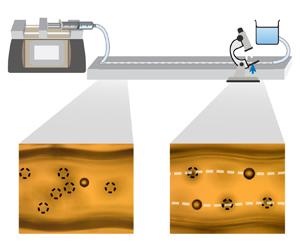
In this paper, we analytically and experimentally investigate the underlying mechanisms that drive focusing behaviour of neutrally buoyant particles in a wavy channel (figure 1). We provide a theoretical analysis for a particle that has an asymptotically small dimension compared with the channel width, as summarized in figure 2. To this end, we first calculate the flow in the wavy channel in the absence of particles, i.e. the particle-free flow or undisturbed flow. Throughout this paper, ‘disturbance/perturbation’ refers to the impact of particles on the particle-free flow. By incorporating the particle-free velocity field into the method of matched asymptotic analysis, we then calculate the inertial lift force on a neutrally buoyant particle in the wavy channel. We simulate the trajectory of the particle and predict focusing locations with a modified Maxey–Riley equation, incorporating source terms including the Stokes drag, fluid acceleration, added mass and lift force on the particle. We reveal the critical role of the inertial lift force in particle focusing and demonstrate different focusing behaviours than those observed in straight channels. By conducting experiments using particles that have finite dimensions compared with the channel width, we not only validate our predictions of the focusing locations but also reveal conditions in which realistic focusing behaviour deviates from the asymptotic analysis.

Figure 2. Structure of the paper. Throughout this work, perturbation refers to the impact of the particle on the particle-free flow.
The paper is organized as follows: in § 2, we calculate the particle-free flow in the wavy channel. In § 3, we formulate the governing equations for the perturbations introduced by an asymptotically small neutrally buoyant particle. In § 4, we calculate the inertial lift force on the particle with matched asymptotic analysis. In § 5, we simulate the trajectory of the particle and predict its focusing locations. In § 6, we experimentally validate our predictions of the focusing locations, explore the focusing conditions and establish the differences in the focusing behaviour between wavy and straight channels. In § 7, we introduce a scaling analysis to qualitatively compare the relative importance between the inertial lift and oscillatory straining effects, revealing how such competition leads to the variation of the focusing locations of particles in different parameter regimes.
2. Particle-free flow
We begin by computing the laminar particle-free velocity field in a two-dimensional wavy channel that extends infinitely in the out-of-plane direction. Consider fluid flow between two symmetric wavy plates with an average separation of  $l$, as shown in figure 3. The wavy plates have a sinusoidal profile with amplitude
  $\epsilon _{w}h$ and wavelength
  $\lambda$, where
  $h$ is the mean half-width of the channel,
  $h=l/2$. We denote the angular frequency of the waviness as
  $\omega ^{\prime }$, i.e.
  $\lambda =2{\rm \pi} /\omega ^{\prime }$; additionally, we assume
  $\lambda$ is at least of
  $O(h)$. The laboratory frame is chosen with an origin located at the intersection between the middle plane and a cross-section on which the channel is of minimum width. We use the coordinate
  $\boldsymbol {\mathcal {R}}^{\prime }=(\mathcal {X}^{\prime },\mathcal {Y}^{\prime },\mathcal {Z}^{\prime })$ for the laboratory frame. The flow is driven by a pressure gradient in the
  $\mathcal {X}^{\prime }$ direction, and the velocity on the middle plane has an average magnitude of
  $U_{m}^{\prime }$.

Figure 3. Schematics of the flow in a wavy channel and two sets of coordinate systems. The solid and dashed velocity profiles represent the actual flow at  $\mathcal {X}^{\prime }=0$ and the zeroth-order plane Poiseuille flow, respectively.
We non-dimensionalize our variables by normalizing the particle-free velocity  $\bar {\boldsymbol {\mathcal {V}}}^{\prime }$ with
  $U_{m}^{\prime }$ and by introducing
  $\boldsymbol {\mathcal {R}}=\boldsymbol {\mathcal {R}}^{\prime }/h=(\mathcal {X},\mathcal {Y},\mathcal {Z})$. In the rest of the paper, dimensionless variables are indicated by a lack of primes. The particle-free fluid pressure
  $\bar {\mathcal {P}}^{\prime }$ is normalized with
  $\rho U_m^{\prime 2}$, where
  $\rho$ is the fluid density. The dimensionless governing equations of
  $\bar {\boldsymbol {\mathcal {V}}}$ can then be written as the dimensionless Navier–Stokes equations and the continuity condition
 $$\begin{gather} \bar{\boldsymbol{\mathcal{V}}} \boldsymbol{\cdot} \boldsymbol{\nabla} \bar{\boldsymbol{\mathcal{V}}} ={-}\boldsymbol{\nabla} \bar{\mathcal{P}} + \frac{2}{R_c} \nabla^2\bar{\boldsymbol{\mathcal{V}}}, \end{gather}$$
 $$\begin{gather}\boldsymbol{\nabla} \boldsymbol{\cdot} \bar{\boldsymbol{\mathcal{V}}} = 0, \end{gather}$$
where  $\bar {\mathcal {P}}$ is the dimensionless particle-free fluid pressure,
  $R_c=2U_{m}^{\prime } h/\nu$ is the channel Reynolds number (Schonberg & Hinch Reference Schonberg and Hinch1989; Hogg Reference Hogg1994; Asmolov Reference Asmolov1999) and
  $\nu$ is the kinematic viscosity of the fluid. The velocity
  $\bar {\boldsymbol {\mathcal {V}}}$ is subject to a no-slip boundary condition on the walls
 \begin{equation} \bar{\boldsymbol{\mathcal{V}}} = 0 \quad \mbox{at} \ \mathcal{Z}={\pm}{1} \mp \epsilon_{w} \,{\rm Re}[\mbox{exp}(\mbox{i}\omega\mathcal{X})], \end{equation}
where  $\omega = \omega ^{\prime }h$. For a small waviness amplitude, i.e.
  $\epsilon _{w} \ll 1$, the particle-free velocity and pressure can be expressed as a series of higher-order corrections to Poiseuille flow
 \begin{equation} \bar{\boldsymbol{\mathcal{V}}} = \bar{\boldsymbol{\mathcal{V}}}^{(0)} + \epsilon_{w}\bar{\boldsymbol{\mathcal{V}}}^{(1)} + O(\epsilon_{w}^{2}) \quad \mbox{and} \quad \bar{\mathcal{P}} = \bar{\mathcal{P}}^{(0)} + \epsilon_{w}\bar{\mathcal{P}}^{(1)} + O(\epsilon_{w}^{2}), \end{equation}
where the  $\mathcal {X}$-component of the zeroth-order particle-free velocity is
  $\bar {\mathcal {V}}_{x}^{(0)}=1-\mathcal {Z}^2$, the
  $\mathcal {Z}$-component of the zeroth-order particle-free velocity is
  $\bar {\mathcal {V}}_{z}^{(0)}=0$ and the zeroth-order particle-free pressure
  $\bar {\mathcal {P}}^{(0)}$ varies linearly in the
  $\mathcal {X}$ direction. Note that this expansion is distinct from the standard lubrication approach in which
  $\epsilon _w h/\lambda \ll 1$. Here, we instead allow for the case where the amplitude of the waviness may be of the same order as the wavelength.
To solve the first-order particle-free flow, we employ a strategy introduced by Van Dyke in 1975; instead of enforcing the no-slip condition at the wavy wall, we transfer the boundary condition in (2.2) to the average locations of the walls (Van Dyke Reference Van Dyke1975; Selvarajan, Tulapurkara & Vasanta Ram Reference Selvarajan, Tulapurkara and Vasanta Ram1998, Reference Selvarajan, Tulapurkara and Vasanta Ram1999) such that the no-slip condition is enforced at the wall to first order. To this end, we write (2.2) as a Taylor series around  $\mathcal {Z}=1$ and then expand
  $\bar {\mathcal {V}}$ and its derivatives in orders of
  $\epsilon _w$ with (2.3a,b), finally arriving at
 $$\begin{gather} \bar{\boldsymbol{\mathcal{V}}}_{x}^{(1)} \simeq{\pm} [\bar{\boldsymbol{\mathcal{V}}}_{x}^{(0)}]^{\prime}{\rm Re}[\mbox{exp}(\mbox{i}\omega\mathcal{X})] \quad \mbox{and} \end{gather}$$
 $$\begin{gather}\bar{\boldsymbol{\mathcal{V}}}_{z}^{(1)} \simeq{\pm} [\bar{\boldsymbol{\mathcal{V}}}_{z}^{(0)}]^{\prime}{\rm Re}[\mbox{exp}(\mbox{i}\omega\mathcal{X})] \quad \mbox{at}\ \mathcal{Z}=\pm1, \end{gather}$$
where the prime symbols denote derivatives with respect to  $\mathcal {Z}$.
We now return to (2.1) to solve for the first-order velocity  $\bar {\boldsymbol {\mathcal {V}}}^{(1)}$ and pressure
  $\bar {\boldsymbol {\mathcal {P}}}^{(1)}$. Inserting (2.3a,b) into (2.1) gives rise to the first-order governing equations, which are then solved with the transferred boundary condition (2.4). The first-order problem is linear in
  $\bar {\boldsymbol {\mathcal {V}}}^{(1)}$ and
  $\bar {\boldsymbol {\mathcal {P}}}^{(1)}$; additionally,
  $\mathcal {X}$ and
  $\mathcal {Z}$ are separated in the transferred boundary conditions (2.4). Thus, we perform separation of variables and make the ansatz
  $\bar {\boldsymbol {\mathcal {V}}}^{(1)}={\rm Re}[\hat {\boldsymbol {\mathcal {V}}}(\mathcal {Z}) \exp (\mbox {i}\omega \mathcal {X})]$ and
  $\bar {\mathcal {P}}^{(1)}={\rm Re}[\hat {\mathcal {P}}(\mathcal {Z}) \exp (\mbox {i}\omega \mathcal {X})]$ following the structure of (2.4). Herein,
  $\hat {\boldsymbol {\mathcal {V}}}(\mathcal {Z})$ and
  $\hat {\mathcal {P}}(\mathcal {Z})$ are assumed to be complex functions, and the Re symbols ensure that the computed
  $\bar {\boldsymbol {\mathcal {V}}}^{(1)}$ and
  $\bar {\boldsymbol {\mathcal {P}}}^{(1)}$ are real-valued functions. The first-order variables
  $\hat {\boldsymbol {\mathcal {V}}}(\mathcal {Z})$ and
  $\hat {\mathcal {P}}(\mathcal {Z})$ are then subject to the following differential equations and boundary conditions:
 $$\begin{gather} \mbox{i}\omega \hat{\mathcal{V}}_{x} + \frac{ \mbox{d}\hat{\mathcal{V}}_{z}}{\mbox{d}\mathcal{Z}} = 0, \end{gather}$$
 $$\begin{gather}\mbox{i}\omega (1-\mathcal{Z}^2)\hat{\mathcal{V}}_{x} - 2\mathcal{Z}\hat{\mathcal{V}}_{z} ={-}\mbox{i}\omega \hat{\mathcal{P}} + \frac{2}{R_c} \left(-\omega^2 + \frac{\mbox{d}}{\mbox{d}\mathcal{Z}^2} \right)\hat{\mathcal{V}}_{x}, \end{gather}$$
 $$\begin{gather}\mbox{i}\omega (1-\mathcal{Z}^2)\hat{\mathcal{V}}_{z} ={-}\frac{\mbox{d}\hat{\mathcal{P}}}{\mbox{d}\mathcal{Z}} + \frac{2}{R_c} \left(-\omega^2 + \frac{\mbox{d}}{\mbox{d}\mathcal{Z}^2} \right)\hat{\mathcal{V}}_{z}, \end{gather}$$
 $$\begin{gather}\hat{\mathcal{V}}_{x} ={-}2 \quad \mbox{and} \quad \hat{\mathcal{V}}_{z} = 0 \quad \mbox{at} \ \mathcal{Z}={\pm} 1. \end{gather}$$
Note that we drop the Re symbols and the sinusoidal term  $\exp (\mathrm {i}\omega \mathcal {X})$ in obtaining (2.5). Equation (2.5) can be solved numerically with the orthonormalization method (Conte Reference Conte1966; Scott & Watts Reference Scott and Watts1977). To avoid numerical instability, we perform integration from both boundaries and match the results at
  $\mathcal {Z}=0$. In short, we solve (2.5) on two intervals,
  $\mathcal {Z}\in [-1,0]$ and
  $\mathcal {Z}\in [0,1]$. For each interval, we write the solution as the summation of a particular solution and a linear combination of orthonormal homogeneous solutions, where the pre-factors for the homogeneous solutions are the unknowns. We integrate (2.5) from both boundaries
  $\mathcal {Z}=\pm 1$, and finally determine the pre-factors by utilizing the continuity of the functional values at
  $\mathcal {Z}=0$.
Figure 4 shows the particle-free velocity field in a wavy channel. Unlike the zeroth-order flow which is independent of the  $\mathcal {X}$-coordinate (figure 4a), the first-order velocity varies periodically along the
  $\mathcal {X}$-direction (figure 4b). Due to the waviness, a pair of counter-rotating vortices appear in both the
  $\mathcal {X}$- and
  $\mathcal {Z}$-directions in each period of the channel. To better illustrate the distributions of
  $\bar {\mathcal {V}}_{x}^{(1)}$ and
  $\bar {\mathcal {V}}_{z}^{(1)}$ across the channel, we select the cross-section
  $\mathcal {X}=0$ and show
  $\bar {\mathcal {V}}_{x}^{(1)}(\mathcal {X}=0)$ and
  $\bar {\mathcal {V}}_{z}^{(1)}(\mathcal {X}=0)$ as functions of
  $\mathcal {Z}$ at varying channel Reynolds number
  $R_c$ (figure 4c) and frequency
  $\omega$ (figure 4d). The first-order
  $x$-velocity correction,
  $\bar {\mathcal {V}}_{x}^{(1)}(\mathcal {X}=0,\mathcal {Z})$ is symmetric about
  $\mathcal {Z}=0$, whereas
  $\bar {\mathcal {V}}_{z}^{(1)}(\mathcal {X}=0,\mathcal {Z})$ is anti-symmetric. As
  $R_c$ or
  $\omega$ increases,
  $\bar {\mathcal {V}}_{x}^{(1)}$ becomes more uniform, and the magnitude in the middle of the channel decreases; by contrast,
  $\bar {\mathcal {V}}_{x}^{(1)}$ varies more sharply close to the boundaries. The magnitude of
  $\bar {\mathcal {V}}_{z}^{(1)}$ does not vary monotonically with
  $R_c$ (figure 4c). By contrast, the magnitude of
  $\bar {\mathcal {V}}_{z}^{(1)}$ increases with
  $\omega$ (figure 4d). The locations of the maximum and minimum
  $\bar {\mathcal {V}}_{z}^{(1)}$ move toward the boundary of the channel as
  $\omega$ increases. Figures 4(c) and 4(d) indicate that the shear rate close to the boundaries is positively related to
  $R_c$ and
  $\omega$.

Figure 4. Particle-free flow in the wavy channel. The flow field can be approximated as the sum of (a) a zeroth-order Poiseuille flow  $\bar {\boldsymbol {\mathcal {V}}}^{(0)}$ and (b) a first-order flow
  $\bar {\boldsymbol {\mathcal {V}}}^{(1)}$ which introduces eddies. In (b),
  $R_c=10$ and
  $\omega =2$. (c) Variations of the first-order velocity components
  $\bar {\mathcal {V}}_{x}^{(1)}$ and
  $\bar {\mathcal {V}}_{z}^{(1)}$ across the channel at
  $\mathcal {X}=0$ for varying channel Reynolds numbers
  $R_c$, where
  $\omega =2$. (d) Variations of the first-order velocity components
  $\bar {\mathcal {V}}_{x}^{(1)}$ and
  $\bar {\mathcal {V}}_{z}^{(1)}$ across the channel at
  $\mathcal {X}=0$ for varying frequencies
  $\omega$ of the waviness, where
  $R_c=250$. Dashed lines in (c,d) represent analytic solutions in the limits
  $R_c\rightarrow 0$ and
  $\omega \rightarrow 0$, respectively.
Figure 4 also includes the analytic solutions at the asymptotic limits  $R_c\rightarrow 0$ and
  $\omega \rightarrow 0$ in 4(c) and 4(d), respectively. In the Stokes-flow limit, the first-order velocity component
  $\bar {\mathcal {V}}_{x}^{( 1 )}(\mathcal {X} =0,\mathcal {Z} )$ is given by
 \begin{align} \bar{\mathcal{V}}_{x}^{( 1 )}( \mathcal{X} =0,\mathcal{Z} ) =\frac{4\cosh ( \omega \mathcal{Z} ) \left[ -\omega \cosh ( \omega ) +\sinh ( \omega ) \right] +4\omega \mathcal{Z} \sinh ( \omega ) \sinh ( \omega \mathcal{Z} )}{2\omega -\sinh ( 2\omega )}, \end{align}
and  $\bar {\mathcal {V}}_{z}^{( 1 )}(\mathcal {X} =0,\mathcal {Z} )$ is calculated to be zero. As
  $R_c$ decreases, our numerical computations asymptote to these analytic solutions, as shown in figure 4(c). In the limit of an infinitesimal waviness frequency, i.e.
  $\omega \rightarrow 0$, our numerical computations also asymptote to the analytic solutions (figure 4d), where
 \begin{equation} \bar{\mathcal{V}}_{x}^{( 1 )}( \mathcal{X} =0,\mathcal{Z} ) = 1-3\mathcal{Z} ^2 \quad\mathrm{and}\quad\bar{\mathcal{V}}_{z}^{( 1 )}( \mathcal{X} =0,\mathcal{Z} ) =0. \end{equation}
The detailed derivations for the Stokes-flow limit  $R_c \rightarrow 0$ and the lubrication limit
  $\omega \rightarrow 0$ are reported in Appendices A and B.
3. Particle perturbation analysis formulation
We now introduce a spherical particle that gives rise to a perturbation to our particle-free channel flow. Hence, we investigate the perturbation in three dimensions. As shown in figure 3, the particle is located at (dimensional) coordinates  $(\mathcal {X}_{p}^{\prime },\mathcal {Y}_{p}^{\prime },\mathcal {Z}_{p}^{\prime })$ and is moving with a (dimensional) translational velocity
  $\boldsymbol U_{p}^{\prime }=U_{p,x}^{\prime } \boldsymbol {e}_{x}+U_{p,z}^{\prime } \boldsymbol {e}_{z}$, where
  $\boldsymbol {e}_x$ and
  $\boldsymbol {e}_z$ are unit vectors in the
  $x$- and
  $z$-directions, respectively. We define
  $\varphi _p=\omega ^{\prime }\mathcal {X}_p^{\prime }$ as the phase angle corresponding to the
  $\mathcal {X}$-location of the particle (figure 3). To understand the perturbation induced by the particle, we choose a non-inertial frame of reference that is instantaneously located at the particle centre and translates at the particle velocity
  $\boldsymbol {U}_{p}^{\prime }$ (Hogg Reference Hogg1994; Asmolov Reference Asmolov1999; Hood et al. Reference Hood, Lee and Roper2015). Since the particle is free, the net force (including the virtual force due to the acceleration of the frame) acting on the particle is zero in this frame of reference. We use the coordinate
  $\boldsymbol {r}^{\prime }=(x^{\prime },y^{\prime },z^{\prime })$ for the particle frame (figure 3). Let
  $\bar {\boldsymbol {v}}^{\prime }$ denote the particle-free velocity and
  $\bar {p}^{\prime }$ the particle-free pressure in the particle frame; namely, the velocity and pressure fields computed in the previous section are shifted by the (currently unknown) velocity
  $\boldsymbol {U}_p^{\prime }$. The particle-free equations of motion can be written in terms of
  $\bar {\boldsymbol {v}}^{\prime }$ as
 $$\begin{gather} \rho \left( \frac{\partial \boldsymbol{\bar{v}}^{\prime}}{\partial t^{\prime}}+\boldsymbol{\bar{v}}^{\prime}\boldsymbol{\cdot} \boldsymbol{\nabla} \mathrm{'}\boldsymbol{\bar{v}}^{\prime}+\boldsymbol{a}_{p}^{\prime} \right) ={-}\boldsymbol{\nabla} '\bar{p}^{\prime}+\mu \nabla'^2\boldsymbol{\bar{v}}^{\prime}, \end{gather}$$
 $$\begin{gather}\boldsymbol{\nabla} '\boldsymbol{\cdot} \boldsymbol{\bar{v}}^{\prime} = 0, \end{gather}$$
 $$\begin{gather}\boldsymbol{\bar{v}}^{\prime} ={-}\boldsymbol{U}_{p}^{\prime} \quad \mbox{on the walls}, \end{gather}$$
where  $\boldsymbol {a}_{p}^{\prime }$ is the particle acceleration measured in the laboratory frame (Kundu, Cohen & Dowling Reference Kundu, Cohen and Dowling2016). Although (3.1) has been solved in the previous section, we rewrite it here in the particle frame as they will be used below to derive the governing equations for the difference between the disturbed and particle-free velocity fields.
We now consider the equations of motion for the flow field which is perturbed by the presence of the particle. Let  $\boldsymbol {v}'$ (note no overbar) denote the disturbed fluid velocity and
  $p'$ the disturbed pressure in the particle frame. The equations for the disturbed flow take the same form of the Navier–Stokes equations and the continuity condition as (3.1)
 $$\begin{gather} \rho \left( \frac{\partial \boldsymbol{v}^{\prime}}{\partial t^{\prime}}+\boldsymbol{v}^{\prime}\boldsymbol{\cdot} \boldsymbol{\nabla} {'}\boldsymbol{v}^{\prime}+\boldsymbol{a}_{p}^{\prime} \right) ={-}\boldsymbol{\nabla} {'}p^{\prime}+\mu \nabla {'}^2\boldsymbol{v}^{\prime}, \end{gather}$$
 $$\begin{gather}\boldsymbol{\nabla} '\boldsymbol{\cdot} \boldsymbol{v}^{\prime}=0. \end{gather}$$
The boundary conditions include a no-slip boundary condition on the walls, a no-slip boundary condition on the surface of the particle and the absence of perturbation far away from the particle
 $$\begin{gather} \boldsymbol{v}^{\prime} ={-}\boldsymbol{U}_{p}^{\prime}\quad \mbox{on the walls}, \end{gather}$$
 $$\begin{gather}\boldsymbol{v}^{\prime} = \boldsymbol{\varOmega }_{p}^{\prime}\times \boldsymbol{r}^{\prime}\boldsymbol \quad \mbox{at}\boldsymbol\ \left| \boldsymbol{r}^{\prime} \right|=a, \end{gather}$$
 $$\begin{gather}\boldsymbol{v}^{\prime} = \boldsymbol{\bar{v}}^{\prime}\quad\mbox{at} \left| x^{\prime} \right|\rightarrow \infty, \end{gather}$$
where  $a$ is the particle radius, and
  $\boldsymbol {\varOmega }_p^{\prime }$ is the particle's rotational velocity. Next, we define the perturbation velocity
  $\boldsymbol {u}^{\prime }$ as the difference between the disturbed and the particle-free velocities, i.e.
  $\boldsymbol {u}^{\prime }=\boldsymbol {v}{'}-\boldsymbol {\bar {v}}{'}$. The governing equations of
  $\boldsymbol {u}^{\prime }$ can be obtained by subtracting (3.1) from (3.2)
 $$\begin{gather} \frac{\partial \boldsymbol{u}^{\prime}}{\partial t^{\prime}}+\boldsymbol{u}^{\prime}\boldsymbol{\cdot} \boldsymbol{\nabla} {'}\boldsymbol{u}^{\prime}+\boldsymbol{\bar{v}}^{\prime}\boldsymbol{\cdot} \boldsymbol{\nabla} {'}\boldsymbol{u}^{\prime}+\boldsymbol{u}^{\prime}\boldsymbol{\cdot} \boldsymbol{\nabla} {'}\boldsymbol{\bar{v}}^{\prime} ={-}\frac{1}{\rho}\boldsymbol{\nabla} {'}(p^{\prime}-\bar{p}^{\prime}) +\nu \nabla{'}^2\boldsymbol{u}^{\prime}, \end{gather}$$
 $$\begin{gather}\boldsymbol{\nabla} {'}\boldsymbol{\cdot} \boldsymbol{u}^{\prime} = 0. \end{gather}$$
Note that the particle acceleration  $\boldsymbol {a}_p^{\prime }$ in (3.1) and (3.2) cancels out during subtraction. The boundary conditions of (3.4) are
 $$\begin{gather}
\boldsymbol{u}^{\prime}=0 \quad \mbox{at} \
z^{\prime}=\left\{\begin{array}{@{}l}-\mathcal{Z}_p^{\prime}-h+\epsilon_{w}h\,{\rm
Re}\{ \exp [ \mathrm{i}(\omega^{\prime} x^{\prime}+\varphi_p ) ] \} \\
h-\mathcal{Z}_p^{\prime}-\epsilon_{w}h\,{\rm Re} \{
\exp [ \mathrm{i}(\omega^{\prime} x^{\prime}+\varphi_p ) ]\} \\ \end{array},\right.
\end{gather}$$
$$\begin{gather}
\boldsymbol{u}^{\prime}=0 \quad \mbox{at} \
z^{\prime}=\left\{\begin{array}{@{}l}-\mathcal{Z}_p^{\prime}-h+\epsilon_{w}h\,{\rm
Re}\{ \exp [ \mathrm{i}(\omega^{\prime} x^{\prime}+\varphi_p ) ] \} \\
h-\mathcal{Z}_p^{\prime}-\epsilon_{w}h\,{\rm Re} \{
\exp [ \mathrm{i}(\omega^{\prime} x^{\prime}+\varphi_p ) ]\} \\ \end{array},\right.
\end{gather}$$
 $$\begin{gather}\boldsymbol{u}^{\prime}=\boldsymbol{\varOmega }_{p}^{\prime}\times \boldsymbol{r}^{\prime}-\boldsymbol{\bar{v}}^{\prime}\quad\mbox{at}\ \left| \boldsymbol{r}^{\prime} \right|=a, \end{gather}$$
 $$\begin{gather}\boldsymbol{u}^{\prime}=\boldsymbol{0}\quad \mbox{at}\ \left| x^{\prime} \right|\rightarrow \infty. \end{gather}$$
We non-dimensionalize (3.5) by introducing
 \begin{equation} \left.\begin{gathered} \boldsymbol{r}=\frac{\boldsymbol{r}^{\prime}}{a},\quad \boldsymbol{u}=\frac{\boldsymbol{u}^{\prime}}{U_{m}^{\prime}},\quad \bar{\boldsymbol{v}}=\frac{\bar{\boldsymbol{v}}^{\prime}}{U_{m}^{\prime}},\quad \omega =\omega ^{\prime}h,\\ \boldsymbol{\varOmega }_p=\frac{2h\boldsymbol{\varOmega }_{p}^{\prime}}{U_{m}^{\prime}},\quad \mbox{and}\quad q=\left( \frac{\mu U_{m}^{\prime}}{a} \right) ^{{-}1}\left( p^{\prime}-\bar{p}^{\prime} \right), \end{gathered}\right\}\end{equation}
where  $\bar {\boldsymbol {v}}$ is the dimensionless particle-free velocity in the particle frame,
  $q$ is the dimensionless perturbation pressure and a lack of prime denotes dimensionless variables. Additionally, we introduce a particle Reynolds number
  $R_p=U_{m}^{\prime }a{{^2}/{( l\nu )}}$ (Schonberg & Hinch Reference Schonberg and Hinch1989; Hogg Reference Hogg1994; Asmolov Reference Asmolov1999), where
  $\nu$ is the kinematic viscosity of the fluid. We define
  $\epsilon =R_{p}^{{{1}/{2}}}=R_{c}^{{{1}/{2}}}{{a}/{l}}$ (Asmolov Reference Asmolov1999; Matas et al. Reference Matas, Morris and Guazzelli2009). This small dimensionless parameter
  $\epsilon$ is taken to be the asymptotic parameter that we will use to analyse the perturbation introduced by the particle, and we assume
  $\epsilon \ll 1$. Hence, we have the following dimensionless governing equations of
  $\boldsymbol {u}$:
 $$\begin{gather} {\epsilon R}_{c}^{{{1}/{2}}}\left( \frac{\partial \boldsymbol{u}}{\partial t}+\boldsymbol{u}\boldsymbol{\cdot} \boldsymbol{\nabla} \boldsymbol{u}+\boldsymbol{\bar{v}}\boldsymbol{\cdot} \boldsymbol{\nabla} \boldsymbol{u}+\boldsymbol{u}\boldsymbol{\cdot} \boldsymbol{\nabla} \boldsymbol{\bar{v}} \right) ={-}\boldsymbol{\nabla} q+\nabla ^2\boldsymbol{u}, \end{gather}$$
 $$\begin{gather}\boldsymbol{\nabla} \boldsymbol{\cdot} \boldsymbol{u}=0, \end{gather}$$
with boundary conditions
 $$\begin{gather} \boldsymbol{u}= \boldsymbol{0}\quad \mbox{at}\ z = \tfrac{1}{2}\epsilon ^{{-}1}R_{c}^{{{1}/{2}}}({\mp} 1 - \mathcal{Z}_p \pm \epsilon_w \,{\rm Re}\{ \exp [ \mathrm{i}(\varphi_p +x\epsilon \kappa )] \}), \end{gather}$$
 $$\begin{gather}\boldsymbol{u}= {\epsilon R}_{c}^{-{{1}/{2}}}\boldsymbol{\varOmega }_p\times \boldsymbol{r}-\boldsymbol{\bar{v}}\quad\mbox{at}\ \left| \boldsymbol{r} \right|=1, \end{gather}$$
 $$\begin{gather}\boldsymbol{u}=0\quad\mbox{at}\ \left| x \right|\rightarrow \infty, \end{gather}$$
where we replace  $2\omega {R_c^{-{1}/{2}}}$ with
  $\kappa$, and
  $\bar {\boldsymbol {v}}$ is the non-dimensional particle-free flow field in the frame of the particle. Additionally, we factor out
  $\epsilon$ in the exponential term of (3.8a) for mathematical convenience in § 4.2.
Finally, we express the particle-frame-based particle-free velocity  $\boldsymbol {\bar {v}}$ in (3.7) using quantities that have been calculated in § 2. In terms of the dimensionless particle-free velocity
  $\boldsymbol {\bar {\mathcal {V}}}$ in the laboratory frame, and the dimensionless particle velocity
  $\boldsymbol {U}_p$ we have
 \begin{equation} \boldsymbol{\bar{v}}=\boldsymbol{\bar{\mathcal{V}}}-\boldsymbol{U}_p. \end{equation}
We further rewrite the arguments of  $\boldsymbol {\bar {\mathcal {V}}}$,
  $\boldsymbol {\bar {\mathcal {V}}}^{(0)}$,
  $\boldsymbol {\bar {\mathcal {V}}}^{(1)}$ and
  $\hat {\boldsymbol {\mathcal {V}}}$ in terms of the dimensionless coordinates in the particle frame
  $x$,
$x$,  $y$ and
  $z$ with the relationships
  $\mathcal {X}=ax/h+\mathcal {X}_p$ and
  $\mathcal {Z}=az/h+\mathcal {Z}_p$, e.g.
  $\hat {\mathcal {V}}_x( \mathcal {Z} ) =\hat {\mathcal {V}}_x( 2\epsilon zR_{c}^{-{{1}/{2}}}+\mathcal {Z}_p )$. Note that a conversion between
  $\mathcal {Y}$ and
  $y$ is not necessary because the
  $y$-components of both
  $\bar {\boldsymbol {\mathcal {V}}}$ and
  $\boldsymbol {U}_{p}$ are equal to zero, leading to
  $\bar {v}_y = 0$ (3.9); similarly, all
  $y$-components in the rest of this section vanish. Moreover, since the perturbation velocity
  $\boldsymbol {u}$ is influenced by the lag between the particle velocity
  $\boldsymbol {U}_p$ and the particle-free velocity at the instantaneous location of the particle centre
  $\boldsymbol {\bar {\mathcal {V}}}( \boldsymbol {\mathcal {R}} _p( t ) )$, we define a dimensionless particle slip velocity,
  $\boldsymbol {V}_s=\boldsymbol {\bar {\mathcal {V}}}( \boldsymbol {\mathcal {R}} _p( t ) ) -\boldsymbol {U}_p$. Inserting (2.3a,b), the asymptotic expansions for
  $\bar {\boldsymbol {\mathcal {V}}}$ and
  $\bar {\mathcal {P}}$ into (3.9), we find
 \begin{equation} \bar{v}_x=V_{s,x}+\Delta \bar{\mathcal{V}}_{x}^{(0)}+\epsilon _w\Delta \bar{\mathcal{V}}_{x}^{(1)}+O ( \epsilon _{w}^{2} ) ,\quad \bar{v}_z=V_{s,z}+\epsilon _w\Delta \bar{\mathcal{V}}_{z}^{(1)}+O ( \epsilon _{w}^{2} ), \end{equation}
where  $\Delta \bar {\mathcal {V}}_{x}^{(i)}$ represents the difference between the
  $i$th order particle-free velocity at location
  $\boldsymbol {r}=( x,y,z )$ and the
  $i$th-order particle-free velocity at the particle centre
  $(0,0,0)$. Here,
  $\Delta \bar {\mathcal {V}}_{x}^{(0)}=\epsilon \gamma zR_{c}^{-{{1}/{2}}}-4\epsilon ^2z^2R_{c}^{-1}$ and
  $\Delta \bar {\mathcal {V}}_{z}^{(0)}=0$, where
  $\gamma =-4\mathcal {Z}_p$ is the zeroth-order shear rate at the particle centre normalized with a characteristic shear rate,
  $U_{m}^{\prime }/{l}$. Additionally,
 $$\begin{gather} \Delta \bar{\mathcal{V}}_{x}^{(1)}={\rm Re}\{ \hat{\mathcal{V}}_x( 2\epsilon z{R}_{c}^{-{1}/{2}}+ \mathcal{Z}_p ) \exp [\mathrm{i}( \varphi_p+\epsilon x\kappa )] -\hat{\mathcal{V}}_x( \mathcal{Z}_p ) \exp ( \mathrm{i}\varphi_p ) \}, \end{gather}$$
 $$\begin{gather}\Delta \bar{\mathcal{V}}_{z}^{(1)}={\rm Re}\{ \hat{\mathcal{V}}_z( 2\epsilon z{R}_{c}^{-{1}/{2}}+\mathcal{Z}_p ) \exp [\mathrm{i}( \varphi_p+\epsilon x\kappa )] -\hat{\mathcal{V}}_z( \mathcal{Z}_p ) \exp ( \mathrm{i}\varphi_p ) \}. \end{gather}$$
To determine the orders of  $\Delta \bar {\mathcal {V}}_{x}^{(1)}$ and
  $\Delta \bar {\mathcal {V}}_{z}^{(1)}$ in
  $\epsilon$ for later analyses in § 4, we first write the Taylor series expansions of
  $\hat {\mathcal {V}}_x( 2{\epsilon z}R_{c}^{-{{1}/{2}}}+\mathcal {Z}_p )$ and
  $\hat {\mathcal {V}}_z ( 2{\epsilon z}R_{c}^{-{{1}/{2}}}+\mathcal {Z}_p )$ at
  $z=0$ under the condition
  $2{\epsilon z}R_{c}^{-{{1}/{2}}} \ll 1$
 $$\begin{gather} \hat{\mathcal{V}}_x( 2{\epsilon z}R_{c}^{-{1}/{2}}+\mathcal{Z}_p ) =\hat{\mathcal{V}}_{x0}+\alpha _x{\epsilon z}R_{c}^{-{1}/{2}}+\tfrac{1}{2}\beta _x\epsilon ^2z^2{R}_c^{{-}1}+O ( \epsilon ^3 ), \end{gather}$$
 $$\begin{gather}\hat{\mathcal{V}}_z( 2{\epsilon z}R_{c}^{-{1}/{2}}+\mathcal{Z}_p ) =\hat{\mathcal{V}}_{z0}+\alpha _z{\epsilon z}R_{c}^{-{1}/{2}}+\tfrac{1}{2}\beta _z\epsilon ^2z^2{R}_c^{{-}1}+O ( \epsilon ^3 ), \end{gather}$$
where  $\hat {\mathcal {V}}_{x0}=\hat {\mathcal {V}}_x( \mathcal {Z}_p )$,
  $\hat {\mathcal {V}}_{z0}=\hat {\mathcal {V}}_z( \mathcal {Z}_p )$ and
  $\alpha _x$,
  $\alpha _z$,
  $\beta _x$ and
  $\beta _z$ are prefactors of the Taylor series, which can be determined numerically from the solutions to (2.5). Specifically, the continuity condition gives rise to the relation
  ${\mathrm {i}\kappa }R_c^{{{1}/{2}}}\hat {\mathcal {V}}_{x0}+\alpha _z=0$. Given (3.12), we further expand
  $\Delta \bar {\mathcal {V}}_{x}^{(1)}$ and
  $\Delta \bar {\mathcal {V}}_{z}^{(1)}$ in Taylor series with respect to both
  $x$ and
  $z$, and find that
  $\Delta \bar {\mathcal {V}}_{x}^{(1)}$ and
  $\Delta \bar {\mathcal {V}}_{z}^{(1)}$ are of
  $O ( \epsilon )$, e.g.
  $\Delta \bar {\mathcal {V}}_{x}^{( 1 )}=\mathrm {Re}[ ( \mathrm {i}x\kappa \hat {\mathcal {V}} _{x0}+\alpha _{x} z R_{c}^{-1/2} ) \exp \mathrm {(i}\varphi _p) ] \epsilon +O(\epsilon ^2)$. These expressions will be used to express the boundary conditions order by order at the surface of a particle in the following section. Furthermore, we can analytically obtain the variables in (3.11) and (3.12) in the lubrication limit where the angular frequency
  $\omega \rightarrow 0$ (Appendix B)
 \begin{equation} \Delta \bar{\mathcal{V}}_{x}^{( 1 )}\rightarrow -12z\epsilon (\mathcal{Z} _pR_{c}^{-{{1}/{2}}}+z\epsilon R_{c}^{{-}1})\cos(\varphi _p) \quad \textrm{and} \quad \Delta \bar{\mathcal{V}}_{z}^{(1)}\rightarrow 0, \end{equation}
which are of  $O(\epsilon )$. We further find in this limit:
 $\hat {\mathcal {V}}_{x0}\rightarrow 1-3\mathcal {Z} _{p}^{2}$,
  $\hat {\mathcal {V}}_{z0}\rightarrow 0$,
  $\alpha _x \rightarrow -12\mathcal {Z} _p$,
  $\alpha _z \rightarrow 0$,
  $\beta _x\rightarrow -24$ and
  $\beta _z\rightarrow 0$.
4. Inertial lift force acting on a neutrally buoyant particle
The particle induces a small perturbation to the steady channel flow and hence experiences an inertial lift force in the lateral direction. In this section, we calculate the inertial lift force on a neutrally buoyant particle (recall that we seek to determine whether particle focusing in wavy channels arises from this lift force). The problem formulated in (3.7) is solved with the method of matched asymptotic expansions (Schonberg & Hinch Reference Schonberg and Hinch1989; Hogg Reference Hogg1994; Asmolov Reference Asmolov1999). We first solve an inner problem to obtain the flow field surrounding the particle. We then regard the particle as a singular point that exerts a force on the channel flow in an outer problem. Finally, matching the inner and outer solutions gives rise to a lift force on the particle.
4.1. Inner solution
We introduce an inner expansion of the perturbation velocity and pressure
 \begin{equation} \boldsymbol{u}=\boldsymbol{u}_0+\epsilon \boldsymbol{u}_1+O ( \epsilon ^2 ) ,\quad q=q_0+\epsilon q_1+O ( \epsilon ^2 ). \end{equation}
Inserting (4.1a,b) into (3.7), the zeroth-order governing equations represent a Stokes-flow problem
 $$\begin{gather} \nabla ^2\boldsymbol{u}_0-\boldsymbol{\nabla} q_0=\boldsymbol{0}, \end{gather}$$
 $$\begin{gather}\boldsymbol{\nabla} \boldsymbol{\cdot} \boldsymbol{u}_0=0, \end{gather}$$
 $$\begin{gather}\boldsymbol{u}_0={-}V_{s,x}\boldsymbol{e}_x-V_{s,z}\boldsymbol{e}_z,\quad \left| \boldsymbol{r} \right|=1, \end{gather}$$
 $$\begin{gather}\boldsymbol{u}_0 \rightarrow \boldsymbol{0},\quad \boldsymbol{r}\rightarrow \infty. \end{gather}$$
In the absence of fluid inertia, we apply Faxén's law and find that  $V_{s,x}$ and
  $V_{s,z}$ are of
  $O(\epsilon ^2{R}_c^{-1})$. Thus, (4.2c) reduces to
  $\boldsymbol {u}_0=\boldsymbol {0}$ on the particle surface, and
  $\boldsymbol {u}_0$ vanishes everywhere in the channel. The first-order governing equations are then
 $$\begin{gather} \nabla ^2\boldsymbol{u}_{1}-\boldsymbol{\nabla} q_{1}=\boldsymbol{0}, \end{gather}$$
 $$\begin{gather}\boldsymbol{\nabla} \boldsymbol{\cdot} \boldsymbol{u}_1=0, \end{gather}$$
 $$\begin{gather}\boldsymbol{u}_1={R}_c^{-{{1}/{2}}}\left( \boldsymbol{\varOmega }_{p}\times \boldsymbol{r}-\gamma z\boldsymbol{e}_{x} \right) - \epsilon _w\epsilon ^{{-}1}\Delta \bar{\mathcal{V}}_{x}^{\left( 1 \right)}\boldsymbol{e}_x - \epsilon _w\epsilon ^{{-}1}\Delta \bar{\mathcal{V}}_{z}^{\left( 1 \right)}\boldsymbol{e}_z,\quad\left| \boldsymbol{r} \right|=1, \end{gather}$$
 $$\begin{gather}\boldsymbol{u}_1\rightarrow \boldsymbol{0},\quad\boldsymbol{r}\rightarrow \infty, \end{gather}$$
where both  $\epsilon ^{-1}\Delta \bar {\mathcal {V}}_{x}^{(1)}$ and
  $\epsilon ^{-1}\Delta \bar {\mathcal {V}}_{z}^{(1)}$ are of
  $O ( 1 )$ (see the end of § 3). We also assume that
  $\epsilon _w$ and
  $\epsilon$ are of the same order of magnitude such that the last two terms in (4.3c) are bounded. The first-order problem is still a Stokes-flow problem. Due to its linearity, (4.3) can be decomposed into several sub-problems, which we solve separately based on the fundamental solutions for a sphere immersed in Stokes flow derived by Guazzelli & Morris (Reference Guazzelli and Morris2011). For a rotational boundary condition with dimensionless rotation rate
  $\boldsymbol {\omega }$ at the particle surface, i.e.
  $\boldsymbol {u}_1=\boldsymbol {\omega } \times \boldsymbol {r}$ at
  $| \boldsymbol {r} |=1$, the perturbation velocity
  $\boldsymbol {u}_1$ is given by
 \begin{equation} \boldsymbol{u}_1=\boldsymbol{\omega }\times \frac{\boldsymbol{r}}{r^3}, \end{equation}
which is adapted from (2.7) in Guazzelli & Morris (Reference Guazzelli and Morris2011). For a straining boundary condition with dimensionless strain-rate tensor  $\boldsymbol{\mathsf{E}}$ at the particle surface, i.e.
  $\boldsymbol {u}_1=\boldsymbol{\mathsf{E}}\boldsymbol {r}$ at
  $| \boldsymbol {r} |=1$, the components of the perturbation velocity
  $\boldsymbol {u}_1$ are given by
 \begin{equation} u_{1i}=\frac{5}{2}\frac{x_i\left( x_j {\mathsf{E}}_{jk}x_k \right)}{r^5}+\frac{1}{2}{\mathsf{E}}_{jk}\left[ \frac{\delta _{ij}x_k+\delta _{ik}x_j}{r^5}-\frac{5x_ix_jx_k}{r^7} \right], \end{equation}
which is adapted from (2.17) in Guazzelli & Morris (Reference Guazzelli and Morris2011). Based on these fundamental solutions, we decompose  $\boldsymbol {u}_1( \boldsymbol {r} )$ into three parts:
  $\boldsymbol {u}_1( \boldsymbol {r} ) =\boldsymbol {u}_{1A}( \boldsymbol {r} ) +\boldsymbol {u}_{1B}( \boldsymbol {r} ) +\boldsymbol {u}_{1C}( \boldsymbol {r} )$ to satisfy the different components in boundary condition (4.3c). In (4.3c), the term
  ${R}_c^{-{{1}/{2}}}( \boldsymbol {\varOmega }_{p}\times \boldsymbol {r} )$ at the boundary corresponds to a pure rotational boundary condition with a dimensionless rotation rate
  $\boldsymbol {\omega }={R}_c^{-{1}/{2}} \boldsymbol {\varOmega }_p$, which gives rise to the solution
 \begin{equation} \boldsymbol{u}_{1A}( \boldsymbol{r} ) ={R}_c^{-{1}/{2}} \boldsymbol{\varOmega }_p\times \frac{\boldsymbol{r}}{r^3}. \end{equation}
The term  $-{R}_c^{-{{1}/{2}}}\gamma z\boldsymbol {e}_{x}$ in (4.3c) represents a simple-shear boundary condition, which can be treated as the combination of a rotational boundary condition with a dimensionless rotation rate
  $\boldsymbol {\omega }=-{R}_c^{-{1}/{2}} (\gamma /2) \boldsymbol {e}_y$ and a straining boundary condition with a dimensionless strain-rate tensor
 \begin{equation} \boldsymbol{\mathsf{E}}={-}\tfrac{1}{2} {R}_c^{-{1}/{2}} \left[ \begin{matrix} 0 & 0 & \gamma\\ 0 & 0 & 0\\ \gamma & 0 & 0\\ \end{matrix} \right]. \end{equation}
We then construct the following solution:
 \begin{equation} \boldsymbol{u}_{1B}( \boldsymbol{r} ) ={R}_c^{-{1}/{2}}\left[ -\frac{\gamma}{2}\boldsymbol{e}_{y}\times \frac{\boldsymbol{r}}{r^3}+\frac{5}{2}\gamma \boldsymbol{r}xz\left( \frac{1}{r^7}-\frac{1}{r^5} \right) -\frac{\gamma}{2r^5}\left( \boldsymbol{e}_{x}z+\boldsymbol{e}_{z}x \right) \right]. \end{equation}
The terms  $-\epsilon _w\epsilon ^{-1}\Delta \bar {\mathcal {V}}_{x}^{( 1 )}\boldsymbol {e}_{x}-\epsilon _w\epsilon ^{-1}\Delta \bar {\mathcal {V}}_{z}^{( 1 )}\boldsymbol {e}_{z}$ in (4.3c) can be treated as the combination of a rotational and a straining boundary condition. Given (3.11), we find the Taylor series for these two terms at the origin and only collect the leading-order terms in
  $\epsilon$. The corresponding strain-rate tensor
  $\boldsymbol{\mathsf{E}}$ and rotation vector
  $\boldsymbol {\omega }$ at the origin can be written as
 \begin{equation} \left.\begin{gathered} \boldsymbol{\mathsf{E}}={-}\epsilon _w{R}_c^{-{1}/{2}}\,{\rm Re}\!\left\{ \exp ( \mathrm{i} \varphi_p ) \left[ \begin{matrix} -\alpha _z & 0 & \dfrac{\zeta}{2}\\[4pt] 0 & 0 & 0\\ \dfrac{\zeta}{2} & 0 & \alpha _z \end{matrix} \right] \right\} \\ \mbox{and} \\ \boldsymbol{\omega }={-}\epsilon _w{R}_c^{-{1}/{2}}\,{\rm Re}\!\left\{ \exp ( \mathrm{i}\varphi_p ) \left[ \begin{array}{@{}c@{}} 0\\ \dfrac{\sigma}{2}\\[4pt] 0 \end{array} \right] \right\}, \end{gathered}\right\} \end{equation}
where  $\zeta := \alpha _x+\mathrm {i}\kappa R_{c}^{1/2}\hat {\mathcal {V}}_{z0}$ and
  $\sigma := \alpha _x-{\mathrm {i}\kappa R}_c^{{{1}/{2}}}\hat {\mathcal {V}}_{z0}$, which reduces to
  $\zeta = \sigma = -12\mathcal {Z}_p$ for an infinitesimal angular frequency
  $\omega$. The third component of the first-order velocity field
  $\boldsymbol {u}_{1C}( \boldsymbol {r} )$ is thus given by
 \begin{align} \boldsymbol{u}_{1C}( \boldsymbol{r} ) &=\epsilon _w{R}_c^{-{1}/{2}}\,{\rm Re}\!\left\{ \exp( \mathrm{i}\varphi_p ) \left[ \left( -\frac{\sigma}{2}\boldsymbol{e}_{y} \right) \times \frac{\boldsymbol{r}}{r^3} +\frac{5}{2}\boldsymbol{r}\left( \zeta xz-\alpha _zx^2+\alpha _zz^2 \right) \left( \frac{1}{r^7}-\frac{1}{r^5} \right)\right.\right. \nonumber\\ &\quad \left.\left. -\frac{\zeta}{2}\left( \frac{z\boldsymbol{e}_{x}+x\boldsymbol{e}_{z}}{r^5} \right) +\alpha _z\left( \frac{x\boldsymbol{e}_{x}-z\boldsymbol{e}_{z}}{r^5} \right) \right] \right\}. \end{align}
We now determine the rotation velocity  $\boldsymbol {\varOmega }_p$ by establishing the balance of moment on the particle. According to Faxén's second law, the leading-order dimensional hydrodynamic torque on the particle
  $\boldsymbol {T}^{\prime }$ is proportional to the relative rotation velocity between the undisturbed flow and the particle (Guazzelli & Morris Reference Guazzelli and Morris2011)
 \begin{equation} \boldsymbol{T}^{\prime}=8{\rm \pi} \mu a^3( \boldsymbol{\bar{\varOmega}}^{\prime}(\boldsymbol{r}^{\prime}=\boldsymbol{0})-\boldsymbol{\varOmega}_{p}^{\prime} ), \end{equation}
where  $\boldsymbol {\bar {\varOmega }}^{\prime }( \boldsymbol {r}^{\prime }=\boldsymbol {0} ) =\boldsymbol {\nabla } ^{\prime }\times {{\bar {\boldsymbol {v}}^{\prime }}/{2}}$ is the rotation vector of the undisturbed flow evaluated at the particle centre. The torque leads to the angular acceleration of the particle, i.e.
  $\boldsymbol {T}^{\prime }=I_p\,\mathrm {d}\boldsymbol {\varOmega }_{p}^{\prime }/{\mathrm {d}}t^{\prime }$, where
  $I_p=(2/5) a^2 m_p$ is the moment of inertia of the particle. Since we assume that the wavelength of the channel
  $\lambda$ is at least of
  $O(l)$, the characteristic time scale
  $t^{\prime }$ for the variation of
  $\boldsymbol {\varOmega }_{p}^{\prime }$ is taken to be
  $l/U_m^{\prime }$. Further normalizing the rotation vectors with
  $U_m^{\prime }/l$ (3.6), we can establish the following moment balance on the neutrally buoyant particle:
 \begin{equation} \frac{1}{15}\epsilon ^2\frac{\mathrm{d}\boldsymbol{\varOmega }_p}{\mathrm{d}t}=\boldsymbol{\bar{\varOmega}}(\boldsymbol{r}=\boldsymbol{0})-\boldsymbol{\varOmega }_p. \end{equation}
Expanding  $\boldsymbol {\varOmega }_p$ into orders of
  $\epsilon$, we find
  $\boldsymbol {\varOmega }_p^{(0)}=\boldsymbol {\bar {\varOmega }}(\boldsymbol {r}=\boldsymbol {0})$. Namely, in the framework of the first-order perturbation analysis in
  $\epsilon$, the particle follows the rotation of the undisturbed flow at the instantaneous particle centre, exerting no net hydrodynamic torque on the fluid. Therefore, the summation of all rotational components in
  $\boldsymbol {u}_1( \boldsymbol {r} )$ must vanish, and
  $\boldsymbol {\varOmega }_p^{(0)}$ equals
  $\{ \gamma +\epsilon _w\,\textrm {Re}[ \exp ( \mathrm {i}\varphi _p ) \sigma ] \} \boldsymbol {e}{{_y}/{2}}$. Instead of a lift force, the perturbation velocity
  $\boldsymbol {u}_1( \boldsymbol {r} )$ leads to a strainlet (or force dipole) on the particle. The truncated term
  $\boldsymbol {\varOmega }_p - \boldsymbol {\varOmega }_p^{(0)}$ generates a rotlet, but its strength is negligible compared with the strainlet. To give a sense of the perturbation velocity field associated with the strainlet, figure 5 shows the distributions of the
  $x$ and
  $z$ components of
  $\boldsymbol {u}_{1}(\boldsymbol {r})$ on the plane
  $y=0$ in the particle frame. Furthermore, at the limit
  $\epsilon _w \rightarrow 0$, our analytic expression of
  $\boldsymbol {u}_{1}(\boldsymbol {r})$ recovers the corresponding expression in a straight channel (see (5.3) in Asmolov Reference Asmolov1999).

Figure 5. Distributions of the (a)  $x$-component and (b)
  $z$-component of the first-order perturbation velocity
  $\boldsymbol {u}_{1}(\boldsymbol {r})$ on the plane
  $y=0$, where
  $\boldsymbol {r}=(x,y,z)$ denotes the coordinate system in the particle frame. Arrows represent the vector field
  $\boldsymbol {u}_{1}(\boldsymbol {r})$, and the circle represents the particle surface. In this example,
  $R_c=100$,
  $\omega =2$,
  $\mathcal {Z}_p=0.5$,
  $\varphi _p=0.3$ and
  $\epsilon _w=0.05$.
4.2. Outer solution
To find the lift force, we now turn to the outer region in which the balance between the viscous and inertial effects are important. In the outer problem, we introduce outer coordinates  $\boldsymbol {R}=( X,Y,Z )$ that are related to the inner variables via
  $\boldsymbol {R}=\epsilon \boldsymbol {r}$. The perturbation velocity and pressure fields are then expressed as
  $\boldsymbol {U}(\boldsymbol {R})$ and
  $P(\boldsymbol {R})$, respectively.
To match the inner and outer problems, we regard the particle as a singular point that exerts a strainlet on the flow field. We will introduce the strainlet as a forcing term at the origin in the momentum equations of the outer problem. To this end, we first convert  $\boldsymbol {u}_1( \boldsymbol {r} )$ (see (4.6)–(4.10)) to a function of outer coordinates
 \begin{align}
\boldsymbol{u}_1(\boldsymbol{R} ) =\frac{5}{2}\epsilon
^2{R}_c^{-{1}/{2}}\frac{\boldsymbol{R}}{R^5}\{ -\gamma
XZ+\epsilon _w\,{\rm Re}[ \exp ( \mathrm{i}\varphi_p
) ( -\zeta XZ+\alpha _zX^2-\alpha _zZ^2)]\} +O( \epsilon ^4 ).
\end{align}
\begin{align}
\boldsymbol{u}_1(\boldsymbol{R} ) =\frac{5}{2}\epsilon
^2{R}_c^{-{1}/{2}}\frac{\boldsymbol{R}}{R^5}\{ -\gamma
XZ+\epsilon _w\,{\rm Re}[ \exp ( \mathrm{i}\varphi_p
) ( -\zeta XZ+\alpha _zX^2-\alpha _zZ^2)]\} +O( \epsilon ^4 ).
\end{align}
Given (4.1a,b) and (4.13), we now propose an outer expansion of the perturbation field
 \begin{equation} \boldsymbol{u}=\epsilon ^3\boldsymbol{U}+O ( \epsilon ^4 ) ,\quad q=\epsilon ^4Q+O ( \epsilon ^5 ). \end{equation}
For a general strain tensor  $\boldsymbol{\mathsf{E}}$ and the corresponding strainlet velocity field
  $\boldsymbol {u}=5x_i {\mathsf{E}}_{ij}x_j{{\boldsymbol {r}}/{( 2r^5 )}}$, the singular forcing term on the right-hand side of the outer momentum equations takes the form of
  $20{\rm \pi} {\mathsf{E}}_{ij}\partial \delta {{( \boldsymbol {r} )}/{\partial x_j}}$ (Hogg Reference Hogg1994). Hence, the governing equations and boundary conditions for our outer problem are
 \begin{align} R_{c}^{\frac{1}{2}}\left(\boldsymbol{\bar{v}}\boldsymbol{\cdot} \boldsymbol{\nabla} \boldsymbol{U} + \boldsymbol{U}\boldsymbol{\cdot} \boldsymbol{\nabla} \boldsymbol{\bar{v}} \right) &=\boldsymbol{\nabla} Q+\nabla ^2\boldsymbol{U}-\frac{10}{3}{\rm \pi} R_{c}^{-{1}/{2}}\gamma \left[ \frac{\partial \delta( \boldsymbol{R} )}{\partial Z}\boldsymbol{e}_x+\frac{\partial \delta( \boldsymbol{R} )}{\partial X}\boldsymbol{e}_z \right]\nonumber\\ &\quad +\epsilon _w\frac{10}{3}{\rm \pi} {R}_c^{-{1}/{2}}\,{\rm Re}\!\left[ \exp( \mathrm{i}\varphi_p ) \left\{ -\zeta \left[ \frac{\partial \delta( \boldsymbol{R} )}{\partial Z}\boldsymbol{e}_x+\frac{\partial \delta( \boldsymbol{R} )}{\partial X}\boldsymbol{e}_z \right]\right.\right.\nonumber\\ &\quad \left.\left. +2\alpha _z\left[ \frac{\partial \delta ( \boldsymbol{R} )}{\partial X}\boldsymbol{e}_x-\frac{\partial \delta ( \boldsymbol{R} )}{\partial Z}\boldsymbol{e}_z \right] \right\} \right] \end{align}
 \begin{equation} \boldsymbol{\nabla} \boldsymbol{\cdot} \boldsymbol{U} = 0 \end{equation}
 \begin{equation} \boldsymbol{U} = \boldsymbol{0} \quad \textrm{at} \ Z =\tfrac{1}{2}R_{c}^{{{1}/{2}}}\left({\mp} 1 - \mathcal{Z}_p \pm \epsilon_w \,{\rm Re}\{\exp [ {\mathrm{i}}\left(\varphi_p +X \kappa \right)] \} \right) .\end{equation}
In obtaining (4.15a), we neglect the time-derivative term. This is because the time scale for the establishment of the disturbance flow,  $l^2/\nu$, is much smaller than the time scale over which the particle migrates laterally relative to the particle-free flow,
  ${{l}/{U_{lateral}}}$ (Hogg Reference Hogg1994). Here,
  $U_{lateral}$ denotes the lateral migration velocity of the particle. We also neglect a term
  $\epsilon ^3\boldsymbol {U}\boldsymbol {\cdot } \boldsymbol {\nabla } \boldsymbol {U}$ in (4.15a), as the interaction of the perturbation flow with itself is negligible compared with other inertial terms. Next, we expand
  ${R}_c^{{{1}/{2}}}\boldsymbol {\bar {v}}$,
  $\boldsymbol {U}$, and
  $Q$ in powers of
  $\epsilon _w$
 $$\begin{gather} {R}_c^{{1}/{2}}\bar{v}_x=\bar{V}_{x}^{\left( 0 \right)}+\epsilon _w\bar{V}_{x}^{\left( 1 \right)}+O ( \epsilon _{w}^{2} ) ,\quad {R}_c^{{1}/{2}}\bar{v}_z=\epsilon _w\bar{V}_{z}^{\left( 1 \right)}+O ( \epsilon _{w}^{2} ), \end{gather}$$
 $$\begin{gather}\boldsymbol{U}=\boldsymbol{U}^{(0)}+\epsilon _w\boldsymbol{U}^{(1)}+O ( \epsilon _{w}^{2} ) , \quad Q=Q^{(0)}+\epsilon _wQ^{(1)}+O ( \epsilon _{w}^{2} ), \end{gather}$$
where  $\bar {V}_{x}^{(0)}=\gamma Z-4Z^2{R}_c^{-{{1}/{2}}}$,
  $\bar {V}_{x}^{(1)}={R}_c^{{{1}/{2}}}\Delta \bar {\mathcal {V}}_{x}^{(1)}$ and
  $\bar {V}_{z}^{( 1 )}={R}_c^{{{1}/{2}}}\Delta \bar {\mathcal {V}}_{z}^{(1)}$ (3.10a,b), which reduce to
  $\bar {V}_{x}^{( 1 )}\rightarrow -12z\epsilon (\mathcal {Z} _p+z\epsilon R_{c}^{-{{1}/{2}}})\cos (\varphi _p)$ and
  $\bar {V}_{z}^{( 1 )}\rightarrow 0$ in the limit
  $\omega \rightarrow 0$. Expanding (4.15) and collecting like terms in
  $\epsilon _w$, we obtain the zeroth-order governing equations and boundary conditions
 \begin{align} &\nabla ^2\boldsymbol{U}^{\left( 0 \right)}-\boldsymbol{\nabla} Q^{\left( 0 \right)}-\bar{V}_{x}^{\left( 0 \right)}\frac{\partial \boldsymbol{U}^{\left( 0 \right)}}{\partial X}-U_{z}^{\left( 0 \right)}\frac{\mbox{d}\bar{V}_{x}^{\left( 0 \right)}}{\mbox{d}Z}\boldsymbol{e}_x \nonumber\\ &\quad={-}\frac{10}{3}{{\rm \pi} R}_c^{-{1}/{2}}\gamma \left[ \frac{\partial \delta( \boldsymbol{R} )}{\partial Z}\boldsymbol{e}_x+\frac{\partial \delta( \boldsymbol{R} )}{\partial X}\boldsymbol{e}_z \right], \end{align}
 \begin{equation} \boldsymbol{\nabla} \boldsymbol{\cdot} \boldsymbol{U}^{\left( 0 \right)}=0, \end{equation}
 \begin{equation} \boldsymbol{U}^{\left( 0 \right)}=\boldsymbol{0},\quad \mbox{at}\ Z_{-}={-}\tfrac{1}{2}{R}_c^{{1}/{2}}( 1+\mathcal{Z}_p ) \quad \mbox{and} \quad Z_+{=}\tfrac{1}{2}{R}_c^{{1}/{2}}( 1-\mathcal{Z}_p ), \end{equation}
 \begin{equation} \boldsymbol{U}^{\left( 0 \right)}=\boldsymbol{0},\quad X\rightarrow \infty, \end{equation}
where  $Z_{-}$ and
  $Z_+$ denote the
  $Z$-coordinates of the average locations of the walls. The first-order governing equations in
  $\epsilon _w$ take the form
 \begin{align} &\nabla ^2\boldsymbol{U}^{(1)}-\boldsymbol{\nabla} Q^{\left( 1 \right)}-\bar{V}_{x}^{\left( 0 \right)}\frac{\partial \boldsymbol{U}^{\left( 1 \right)}}{\partial X}-U_{z}^{\left( 1 \right)}\frac{\mbox{d}\bar{V}_{x}^{\left( 0 \right)}}{\mbox{d}Z}\boldsymbol{e}_{x}=\bar{V}_{x}^{\left( 1 \right)}\frac{\partial \boldsymbol{U}^{\left( 0 \right)}}{\partial X}+\bar{V}_{z}^{\left( 1 \right)}\frac{\partial \boldsymbol{U}^{\left( 0 \right)}}{\partial Z} \nonumber\\ &\quad +\left( U_{x}^{\left( 0 \right)}\frac{\partial \bar{V}_{x}^{\left( 1 \right)}}{\partial X}+U_{z}^{\left( 0 \right)}\frac{\partial \bar{V}_{x}^{\left( 1 \right)}}{\partial Z} \right) \boldsymbol{e}_x+\left( U_{x}^{\left( 0 \right)}\frac{\partial \bar{V}_{z}^{\left( 1 \right)}}{\partial X}+U_{z}^{\left( 0 \right)}\frac{\partial \bar{V}_{z}^{\left( 1 \right)}}{\partial Z} \right) \boldsymbol{e}_z \nonumber\\ &\quad+\frac{10}{3}{{\rm \pi} R}_c^{-{1}/{2}}\,{\rm Re}\!\left[ \exp ( \mathrm{i}\varphi_p ) \left\{ \begin{array}{c} -\zeta \left[ \dfrac{\partial \delta ( \boldsymbol{R} )}{\partial Z}\boldsymbol{e}_x+\dfrac{\partial \delta ( \boldsymbol{R} )}{\partial X}\boldsymbol{e}_z \right] \\[10pt] +2\alpha _z\left[ \dfrac{\partial \delta ( \boldsymbol{R} )}{\partial X}\boldsymbol{e}_x-\dfrac{\partial \delta ( \boldsymbol{R} )}{\partial Z}\boldsymbol{e}_z \right] \end{array} \right\} \right] , \end{align}
 \begin{equation} \boldsymbol{\nabla} \boldsymbol{\cdot} \boldsymbol{U}^{\left( 1 \right)}=0. \end{equation}
Similar to our strategy in (2.4), we transfer the boundary condition (4.15c) to the average locations of the walls instead of enforcing  $\boldsymbol {U}^{(1)}=\boldsymbol {0}$ at the wavy walls, such that
  $\boldsymbol {U}^{(1)}=\boldsymbol {0}$ is enforced at the wavy wall to the first order (Van Dyke Reference Van Dyke1975)
 $$\begin{gather} \boldsymbol{U}^{\left( 1 \right)}={\pm} \frac{1}{2}\frac{\partial \boldsymbol{U}^{\left( 0 \right)}}{\partial Z}{R}_c^{{1}/{2}}\,{\rm Re}\{ \exp [\mathrm{i}( \varphi_p+\kappa X )] \} ,\quad\mbox{at}\ \boldsymbol{R}=\left( X,Y,Z_{{\pm}} \right) \end{gather}$$
 $$\begin{gather}\boldsymbol{U}^{\left( 1 \right)}=\boldsymbol {0},\quad X\rightarrow \infty , \end{gather}$$
where  $Z_{\pm }=\{ Z_{-}, Z_+ \}$ denotes the
  $Z$-coordinates of the average locations of the walls.
4.3. Matching inner and outer solutions
Matching the inner and outer solutions enables us to calculate the lift force on the particle in the  $z$-direction. From (4.1a,b) and (4.14a,b), we know that the perturbation velocity component at the origin
  $u_{z}(\boldsymbol {R}=\boldsymbol {0})$, i.e. the lateral migration velocity of the particle relative to the undisturbed flow, can be determined from the difference between
  $\epsilon ^3 U_z( \boldsymbol {R}=\boldsymbol {0} )$ and
  $\epsilon u_{1,z}( \boldsymbol {R}=\boldsymbol {0} )$. The migration velocity
  $u_{z}(\boldsymbol {R}=\boldsymbol {0})$ gives rise to an inertial lift force acting on the particle in the
  $z$ direction (Schonberg & Hinch Reference Schonberg and Hinch1989; Hogg Reference Hogg1994; Asmolov Reference Asmolov1999) (see derivations of the force balance in Appendix C). Given the characteristic force scale
  $\mu aU_{m}^{\prime }$, the dimensionless lift force on the particle
  $F_{L,z}$ is then
 \begin{equation} F_{L,z}=6{\rm \pi} u_z =6{\rm \pi} \epsilon ^3\lim_{\boldsymbol {R}\rightarrow \boldsymbol {0}} \!( U_z- \epsilon^{{-}2}u_{1,z} ). \end{equation}
Since  $u_{1,z}(\boldsymbol {R})$ has already been obtained in (4.13), we now provide a strategy to numerically solve
  $U_z$. We first convert the partial differential equations (PDEs) (4.17) and (4.18) with Fourier transforms, obtaining governing equations for
  $\boldsymbol {\tilde {U}}^{(0)}(k_x,k_y,Z)$ and
  $\boldsymbol {\tilde {U}}^{(1)}(k_x,k_y,Z)$, where the tildes denote quantities in the frequency domain, and
  $k_x$ and
  $k_y$ are frequencies. We further convert these PDEs into ordinary differential equations (ODEs) for
  $\tilde {U}_z^{(0)}$ and
  $\tilde {U}_z^{(1)}$, respectively. Numerically solving the ODEs for
  $\tilde {U}_z^{(0)}$ and
  $\tilde {U}_z^{(1)}$ and performing inverse Fourier transforms will enable us to obtain
  $F_{L,z}$ at different orders of
  $\epsilon _w$ based on (4.20). The detailed derivations for the ODEs are documented in Appendix D.1.
After solving  $\tilde {U}_{z}^{( 1a )}$ and
  $\tilde {U}_{z}^{( 1b )}$ for arbitrary values of
  $k_x$ and
  $k_y$, we further evaluate the normalized lift force by performing the following inverse Fourier transform:
 $$\begin{gather} F_{L,z} = F_{L,z}^{(0)} + \epsilon _w F_{L,z}^{\left( 1 \right)} + O(\epsilon _w^{2}), \end{gather}$$
 $$\begin{gather}F_{L,z}^{(0)}=6{\rm \pi} \epsilon ^3\,{\rm Re}\!\left[ \int_{-\infty}^{+\infty}{\int_{-\infty}^{+\infty}\tilde{U}_{z}^{\left( 0 \right)}( k_x,k_y,0 )\,\mathrm{d}k_x\,\mathrm{d}k_y} \right], \end{gather}$$
 $$\begin{gather}F_{L,z}^{(1)}=6{\rm \pi} \epsilon ^3\,{\rm Re}\!\left[ \int_{-\infty}^{+\infty}\int_{-\infty}^{+\infty} \tilde{U}_{z}^{\left( 1 \right)}( k_x,k_y,0 ) \,\mathrm{d}k_x\,\mathrm{d}k_y\right]. \end{gather}$$
According to (D6)–(D7),  $\tilde {U}_{z}^{( 1 )}$ can be written in a form with the underlying parameters
  $\mathcal {X}_p$ and
  $\mathcal {Z}_p$ separated
 \begin{align} {\tilde{U}_{z}^{\left( 1 \right)}( k_x,k_y,0 )}=\tfrac{1}{2} [ \exp( \mathrm{i}\varphi_p ) \tilde{U}_{z}^{\left( 1a \right)}( \check{k}_x,k_y,0 ) +\exp ( -\mathrm{i}\varphi_p ) \tilde{U}_{z}^{\left( 1b \right)}( \hat{k}_x,k_y,0 )], \end{align}
where  $\check {k}_x = k_x - \kappa$,
  $\hat {k}_x = k_x + \kappa$ and the particle's coordinate components
  $\mathcal {X}_p$ and
  $\mathcal {Z}_p$ are embedded in
  $\varphi _p$ and
  $\tilde {U}_{z}^{( 1a/b )}$, respectively. Compared with (4.20), (4.21) does not contain any terms from
  $u_{1,z}( \boldsymbol {R}=\boldsymbol {0} )$ (4.13), because the two-dimensional Fourier transform of a strainlet velocity field is imaginary at the origin (Schonberg & Hinch Reference Schonberg and Hinch1989; Hogg Reference Hogg1994; Asmolov Reference Asmolov1999). Thus,
  $F_{L,z}$ is different from the outer solution
  $U_z(\boldsymbol {R}=\boldsymbol {0})$ only by a factor of
  $6{\rm \pi} \epsilon ^3$. Notably,
  $F_{L,z}$ is a function of
  $\mathcal {X}_p$,
  $\mathcal {Z}_p$,
  $\omega$,
  $\epsilon$ and
  $\epsilon _w$.
It is important to note that the ODEs for  $\tilde {U}_{z}^{( 1a )}$ and
  $\tilde {U}_{z}^{( 1b )}$ (D8)–(D12) reduce to the same form in the limit of
  $\omega \rightarrow 0$, giving rise to
  $\tilde {U}_{z}^{( 1a )}( \check {k}_x,k_y,0 ) = \tilde {U}_{z}^{( 1b )}( \hat {k}_x,k_y,0 )$. In this case, one can show that
  $F_{L,z}^{( 1 )}$ is in phase with the sinusoidal profile of the wavy channel (4.22).
We compute  $F_{L,z}^{(0)}$,
  $F_{L,z}^{(1)}$ and
  $F_{L,z}$ across the channel based on (4.21) and present the results in figures 6–8, respectively. Figure 6 shows
  $\epsilon ^{-3}R_{c}^{{{1}/{2}}} F_{L,z}^{(0)}$ as a function of
  $\mathcal {Z}_p$ at varying
  $R_c$. The zeroth-order lift-force component
  $F_{L,z}^{(0)}$ points towards the wall, or outwards, when the particle is in the inner part of the channel;
  $F_{L,z}^{(0)}$ points towards the centreline, or inwards, when the particle gets close to the wall. As
  $R_c$ increases, the equilibrium position of
  $F_{L,z}^{(0)}$ shifts outwards, and the magnitude of
  $\epsilon^{-3} R_c^{1/2}F_{L,z}^{(0)}$ decreases in the inner part of the channel. Our computed zeroth-order lift force is consistent with the lift force reported in Asmolov (Reference Asmolov1999).

Figure 6. Normalized zeroth-order lift force  $\epsilon ^{-3}R_{c}^{{{1}/{2}}}F_{L,z}^{(0)}$ as a function of the
  $\mathcal {Z}$-coordinate of the particle
  $\mathcal {Z}_p$ at varying channel Reynolds numbers
  $R_c$. For varying particle
  $z$-location
  $\mathcal {Z}_p$, the outer solution
  $U_z^{(0)}(\boldsymbol {R}=\boldsymbol {0})$ is different from
  $F_{L,z}^{(0)}$ only by a factor of
  $6{\rm \pi} \epsilon ^3$ (4.21b).

Figure 7. Normalized first-order (in  $\epsilon _w$) lift force. (a,b) Value of
  $\epsilon ^{-3}R_c^{1/2}F_{L,z}^{(1)}$ as a function of the
  $\mathcal {Z}$-coordinate of the particle
  $\mathcal {Z}_p$ and the particle's phase angle in the x-direction
  $\varphi _p$ for (a)
  $R_c=10$,
  $\omega =2$ and (b)
  $R_c=100$,
  $\omega =0.02$. Results for
  $|\mathcal {Z}_p|>1$ are obtained by extrapolation. (c) Value of
  $\epsilon ^{-3}R_{c}^{{{1}/{2}}}F_{L,z}^{(1)}( \varphi _p=0 )$ and
  $\epsilon ^{-3}R_{c}^{{{1}/{2}}}F_{L,z}^{(1)}( \varphi _p={{{\rm \pi} }/{2}} )$ as a function of
  $\mathcal {Z}_p$ at varying
  $R_c$ and
  $\omega =2$. Here, a scaling factor
  $R_c^{1/2}$ makes the order of magnitude consistent for varying
  $R_c$. (d) Value of
  $\epsilon ^{-3}R_{c}^{{{1}/{2}}}F_{L,z}^{(1)}( \varphi _p=0 )$ and
  $\epsilon ^{-3}R_{c}^{{{1}/{2}}}F_{L,z}^{(1)}( \varphi _p={{{\rm \pi} }/{2}} )$ as a function of
  $\mathcal {Z}_p$ at varying
  $\omega$ and
  $R_c=100$. Dashed lines in (d) represent numerical solutions for
  $\omega \rightarrow 0$. For varying particle
  $z$-location
  $\mathcal {Z}_p$, the outer solution
  $U_z^{(1)}(\boldsymbol {R}=\boldsymbol {0})$ is different from
  $F_{L,z}^{(1)}$ only by a factor of
  $6{\rm \pi} \epsilon ^3$ (D6a) and (4.21c).

Figure 8. Normalized lift force  $\epsilon ^{-3}F_{L,z}$ as a function of the
  $\mathcal {Z}$-coordinate of the particle
  $\mathcal {Z}_p$ and the phase angle of the particle in the
  $x$-direction
  $\varphi _p$ for (a)
  $R_c=10$,
  $\omega =2$ and (b)
  $R_c=100$,
  $\omega =0.02$. (c) Zero-lift-force location
  $\mathcal {Z}_p|_{F_{L,z}=0}$ as a function of
  $\varphi _p$ for varying
  $R_c$ and
  $\omega =2$. (d) Zero-lift-force location
  $\mathcal {Z}_p|_{F_{L,z}=0}$ as a function of
  $\varphi _p$ for varying
  $\omega$ and
  $R_c=100$.
  $\epsilon _w=0.05$ for all panels.
The first-order lift force  $F_{L,z}^{(1)}$ varies in both the
  $x$- and
  $z$-directions and is a function of the channel Reynolds number
  $R_c$ and the frequency
  $\omega$. Figures 7(a) and 7(b) show the variation of the normalized first-order lift force
  $\epsilon ^{-3}R_c^{1/2}F_{L,z}^{(1)}$ in a period of the channel for two pairs of
  $R_c$ and
  $\omega$; due to the sharp variations close to the walls, we adopt a moderate range of
  $[-200,200]$ for
  $\epsilon ^{-3}R_c^{1/2}F_{L,z}^{(1)}$ to better illustrate the variations in the bulk of the channel. The lift force
  $F_{L,z}^{(1)}$ has a relatively low magnitude close to the centre of the channel, and its magnitude increases sharply close to the walls. The sign of
  $F_{L,z}^{(1)}$ also varies with the phase angle of the particle in the
  $x$-direction
  $\varphi _p$, where
  $\varphi _p=\omega \mathcal {X}_p$. According to (4.21c), for any particle location,
 \begin{equation} F_{L,z}^{(1)}(\mathcal{X}_p,\mathcal{Z}_p) = \sin ( \varphi_p ) F_{L,z}^{(1)}( \mathcal{X}_p=0,\mathcal{Z}_p ) + \cos ( \varphi_p ) F_{L,z}^{(1)}\left( \mathcal{X}_p=\frac{\rm \pi}{2 \omega} ,\mathcal{Z}_p \right). \end{equation}
Thus, we present  $F_{L,z}^{(1)}$ as a function of
  $\mathcal {Z}_p$ at two phase angles in the
  $x$-direction, i.e.
  $\varphi _p=0$ and
  $\varphi _p={\rm \pi} /2$ in figures 7(c) and 7(d), respectively. Figure 7(c) shows the influence of
  $R_c$ at
  $\omega =2$, and figure 7(d) shows the influence of
  $\omega$ at
  $R_c=100$. Notably, increasing
  $R_c$ and decreasing
  $\omega$ have a similar effect on the
  $\mathcal {Z}_p$–
 $F_{L,z}^{(1)}$ relationship, as illustrated in the resemblance in the variation of the curves between figures 7(c) and 7(d). Figure 7(d) also shows a vanishing
  $F_{L,z}^{(1)}$ for
  $\varphi _p={\rm \pi} /2$ in the limit of
  $\omega \rightarrow 0$, which accords with our observation that
  $F_{L,z}^{(1)}$ is in phase with the wavy channel.
By adding  $F_{L,z}^{(0)}$ and
  $F_{L,z}^{(1)}$, we show the variation of
  $\epsilon ^{-3} F_{L,z}$ across the channel for two pairs of
  $R_c$ and
  $\omega$ in figures 8(a) and 8(b). We are interested in the locations where
  $F_{L,z}=0$, i.e. the zero contour lines. Particles are unstable on the zero contour line at the centre because the nearby lift force points away from the centreline. In figure 8(a), we also observe a pair of unstable zero contour lines along part of the channel close to the walls (mostly within
  $\varphi _p \in [{\rm \pi},2{\rm \pi} ]$). These near-wall zero contour lines arise because
  $F_{L,z}^{(0)}$ and
  $F_{L,z}^{(1)}$ have different signs in these regions and
  $F_{L,z}^{(1)}$ has a large magnitude close to the walls for
  $R_c=10,\omega =2$ (figure 7c). Since previous studies report that the lift force directs particles away from the walls (Asmolov Reference Asmolov1999; Di Carlo et al. Reference Di Carlo, Edd, Humphry, Stone and Toner2009), it is unlikely that particles may be pushed toward the walls as they approach these unstable contour lines. Note that we compute the undisturbed flow and the perturbation velocity up to the first order in
  $\epsilon _w$. Due to the sharp variations in the first-order flow and perturbation fields near the walls, higher-order computations may be necessary for a better understanding of the near-wall lift force, which is, however, beyond the scope of our current analyses. The critical stable zero contour lines are close to
  $\mathcal {Z}_p=\pm 0.6$. The shapes of these stable zero contour lines do not always follow the configuration of the channel. For a large
  $R_c$ and a small
  $\omega$ (figure 8b), the shape of the stable zero contour line is in phase with the configuration of the wavy channel. As
  $R_c$ decreases or
  $\omega$ increases, the shape of the stable zero contour line gradually becomes out of phase, as shown in figures 8(c) and 8(d).
Finally, it is important to note that the zero-lift-force locations are generally different from the focusing locations of particles in wavy channels. Unlike the situation in straight channels where both types of locations coincide, the secondary flow in wavy channels makes particles move in the  $z$-direction constantly. Thus, even if a particle finally stabilizes in a wavy channel, it never truly reaches equilibrium. To resolve the focusing location, it is necessary to analyse the particle trajectory, which we address in § 5.
5. Particle focusing locations
After obtaining the lift force on the particle, we here provide a strategy to predict the focusing locations of the particle in the wavy channel. For this, we come back to the laboratory frame (figure 3). We use  $\boldsymbol {\mathcal {R}}_p^{\prime}( t ) =( \mathcal {X} _p^{\prime}( t ) ,\mathcal {Z} _p^{\prime}( t ) )$ to denote the instantaneous location of the particle centre. Instead of solving the fluid stress over the surface of the particle and using Newton's second law, we employ the modified Maxey–Riley equation to analyse the trajectory of the particle (Maxey & Riley Reference Maxey and Riley1983; Ferry & Balachandar Reference Ferry and Balachandar2001)
 \begin{align} m_p
\frac{\mbox{d}\boldsymbol{U}_{p}^{\prime}}{\mbox{d}t^{\prime}}
&= 6{\rm \pi} a\mu (
\bar{\boldsymbol{\mathcal{V}}}'-\boldsymbol{U}_{p}^{\prime}
)
+m_f\frac{\mbox{D}\bar{\boldsymbol{\mathcal{V}}}'}{\mbox{D}t^{\prime}}+\frac{1}{2}m_f\left(
\frac{\mbox{D}\bar{\boldsymbol{\mathcal{V}}}'}{\mbox{D}t^{\prime}}-\frac{\mbox{d}\boldsymbol{U}_{p}^{\prime}}{\mbox{d}t^{\prime}}
\right) +( m_p-m_f ) \boldsymbol{g}^{\prime}
\nonumber\\ &\quad +\frac{6{\rm \pi}
a^2\mu}{\sqrt{\nu}}\frac{\mbox{d}^{{{1}/{2}}}}{\mbox{d}t^{\prime
{{1}/{2}}}}(
\bar{\boldsymbol{\mathcal{V}}}'-\boldsymbol{U}_{p}^{\prime}
) +\boldsymbol{F}_{L}^{\prime},
\end{align}
\begin{align} m_p
\frac{\mbox{d}\boldsymbol{U}_{p}^{\prime}}{\mbox{d}t^{\prime}}
&= 6{\rm \pi} a\mu (
\bar{\boldsymbol{\mathcal{V}}}'-\boldsymbol{U}_{p}^{\prime}
)
+m_f\frac{\mbox{D}\bar{\boldsymbol{\mathcal{V}}}'}{\mbox{D}t^{\prime}}+\frac{1}{2}m_f\left(
\frac{\mbox{D}\bar{\boldsymbol{\mathcal{V}}}'}{\mbox{D}t^{\prime}}-\frac{\mbox{d}\boldsymbol{U}_{p}^{\prime}}{\mbox{d}t^{\prime}}
\right) +( m_p-m_f ) \boldsymbol{g}^{\prime}
\nonumber\\ &\quad +\frac{6{\rm \pi}
a^2\mu}{\sqrt{\nu}}\frac{\mbox{d}^{{{1}/{2}}}}{\mbox{d}t^{\prime
{{1}/{2}}}}(
\bar{\boldsymbol{\mathcal{V}}}'-\boldsymbol{U}_{p}^{\prime}
) +\boldsymbol{F}_{L}^{\prime},
\end{align}
where  $m_p$ is the particle mass,
  $m_f$ is the fluid mass displaced by the particle,
  $\bar {\boldsymbol {\mathcal {V}}}^{\prime }=\bar {\boldsymbol {\mathcal {V}}}^{\prime }( \bar {\boldsymbol {\mathcal {R}}}_{p}^{\prime }( t ) )$ is the particle-free fluid velocity at the instantaneous particle centre,
  ${{\mathrm {D}}/{\mathrm {D}}}t^{\prime }$ is the material derivative following a fluid parcel,
  $\boldsymbol{g}'$ is the gravitational acceleration and
  $\mu$ is the dynamic viscosity of the fluid. Additionally,
  ${\mbox {d}\boldsymbol {U}_{p}^{\prime }}/{\mbox {d}t^{\prime }}=\boldsymbol {a}_p^{\prime }$ is the particle acceleration defined in § 3. The terms on the right-hand side of (5.1) represent the Stokes drag, fluid acceleration, added mass, gravity, Basset force and lift force on the particle. For the scaling analysis, we choose
  $l$ as the characteristic length,
  $U_{m}^{\prime }$ as the characteristic velocity,
  ${{l}/{U_{m}^{\prime }}}$ as the characteristic time and
  $\mu aU_{m}^{\prime }$ as the characteristic lift force. By comparing the forcing terms, we neglect the Basset force and write (5.1) in the following dimensionless form:
 \begin{align} \left( 1+\frac{1}{2}\frac{\rho _f}{\rho _p} \right) Stk \frac{\mathrm{D}\!\left( \boldsymbol{U}_p-\bar{\boldsymbol{\mathcal{V}}} \right)}{\mathrm{D}t}={-}\left( \boldsymbol{U}_{p}-\bar{\boldsymbol{\mathcal{V}}} \right) +\left( \frac{\rho _f}{\rho _p}-1 \right) Stk \frac{\mathrm{D}\bar{\boldsymbol{\mathcal{V}}}}{\mathrm{D}t}+B\boldsymbol{e}_g+\frac{1}{6{\rm \pi}}\boldsymbol{F}_L, \end{align}
where  $\rho _p$ is the particle density,
  $B=2a^2( \rho _p-\rho _f ) \boldsymbol {g}{{^{\prime }}/{( 9\mu U_{m}^{\prime } )}}$ is the buoyancy number,
  $\boldsymbol {e}_g$ is a unit vector in the direction of the gravitational force and
  $Stk$ is the Stokes number. Specifically,
  $Stk$ is the ratio between the particle relaxation time
  $t_p$ and the characteristic time of the flow
  $t_f$, where
  $t_p=2\rho _p a^2/{( 9\mu )}$ and
  $t_f={{l}/{U_{m}^{\prime }}}$. Since our asymptotic parameter
  $\epsilon =R_{c}^{1/2}a/l={(\rho _f U_m^{\prime }l/\mu )}^{1/2}a/l$, we have
 \begin{equation} Stk=\frac{2}{9}\frac{\rho _p}{\rho _f}\epsilon ^2\ll 1. \end{equation}
For a neutrally buoyant particle, (5.2) can be converted into a differential equation of the particle location
 \begin{equation} \frac{1}{3}\epsilon ^2\ddot{\boldsymbol{\mathcal{R}}}_p+\dot{\boldsymbol{\mathcal{R}}}_p=\bar{\boldsymbol{\mathcal{V}}}+\frac{1}{3}\epsilon ^2 \frac{\mathrm{D}\bar{\boldsymbol{\mathcal{V}}}}{\mathrm{D}t}+\frac{1}{6{\rm \pi}}\boldsymbol{F}_L, \end{equation}
where  $\dot {\boldsymbol {\mathcal {R}}}_p$ and
  $\ddot {\boldsymbol {\mathcal {R}}}_p$ denote the velocity and acceleration of the particle, respectively. Here,
  $\dot {\boldsymbol {\mathcal {R}}}_p=\boldsymbol {U}_p$. With
  $\bar {\boldsymbol {\mathcal {V}}}$ and
  $\boldsymbol {F}_L$ solved in previous sections, we can simulate the trajectory of the particle based on (5.4). By holding
  $R_c$,
  $\omega$, and
  $\epsilon _w$ constant, we find that the simulated trajectory gradually stabilizes over time for any initial particle location. We regard the stabilized trajectory in a period of the channel as particle focusing locations. Additionally, the stabilized trajectory asymptotes to a constant shape as
  $\epsilon$ decreases; as indicated by the stabilized range of the particle's
  $z$-location (inset of figure 9b), the stabilized trajectory for
  $\epsilon = 0.2$ is not significantly different from that for
  $\epsilon = 0.1$.

Figure 9. (a) Simulated trajectories of a particle initially located at  ${\mathcal {Z}}_p=0.1$ in channels with varying amplitude
  $\epsilon _w$, where the lift forces are the zeroth- and first-order lift forces (a-1) and zeroth-order lift force only (a-2). Here,
  $R_c=10$,
  $\omega =2$ and
  $\epsilon =0.2$. (b) Influence of asymptotic parameter
  $\epsilon$ on the simulated trajectory of a particle initially located at
  ${\mathcal {Z}}_p=0.1$, where
  $R_c=10$,
  $\omega =2$,
  $\epsilon _w=0.05$ and the lift force contains both the zeroth- and first-order lift forces. (c) Average focusing location
  $\bar {\mathcal {Z}}_p$ as a function of channel Reynolds number
  $R_c$ for varying
  $\epsilon _w$, where
  $\omega =2$. (d) Average focusing location
  $\bar {\mathcal {Z}}_p$ as a function of channel angular frequency
  $\omega$ for varying
  $\epsilon _w$, where
  $R_c=100$.
In figure 9(a), we show two sets of simulated particle trajectories in channels with amplitudes  $\epsilon _w=0,0.05$ and 0.1 for
  $R_c=10,\omega =2$ and
  $\epsilon =0.2$. The results in figure 9(a-1) are based on both the zeroth-order and first-order lift forces, i.e.
  $F_{L,z}$. For all three values of
  $\epsilon _w$, the particle is initially at
  $\mathcal {Z}_p=0.1$ and gradually migrates towards the stable focusing locations. When
  $\mathcal {X}_p=2000$, the movement of the particle is stabilized: for the straight channel (
 $\epsilon _w=0$),
  $\mathcal {Z}_p$ does not change over time and agrees with the asymptotic solution based on Asmolov (Reference Asmolov1999); for the wavy channels (
 $\epsilon _w=0.05$ and 0.1),
  $\mathcal {Z}_p$ oscillates sinusoidally about an average level. As
  $\epsilon _w$ increases, the amplitude of
  $\mathcal {Z}_p$ also increases but is always lower than
  $\epsilon _w$; additionally, the average focusing location shifts slightly inwards. Interestingly, the channel length for particle focusing is independent of
  $\epsilon _w$, but is significantly impacted by
  $\epsilon$ (figure 9b). We notice that when
  $\epsilon$ becomes very small, e.g.
  $\epsilon =0.01$, a significantly longer channel is required to achieve particle focusing. Because
  $\boldsymbol {F}_L\sim O(\epsilon ^3 )$, a smaller
  $\epsilon$ gives rise to a smaller lift force, which causes the particle to migrate more slowly.
To understand which part of the lift force contributes to the oscillation and shifting of the focusing locations, we only keep the zeroth-order lift force  $F_{L,z}^{(0)}$ and repeat the simulations for the particle trajectories. By comparing the insets of figures 9(a-1) and 9(a-2), we find only slight differences in the average focusing locations for
  $\epsilon _w=0.05$ and 0.1. All other features of figures 9(a-1) and 9(a-2) are indistinguishable. The zeroth-order lift force is thus the governing force for particle focusing in wavy channels. Despite its sinusoidal characteristics, the first-order lift force
  $F_{L,z}^{(1)}$ plays an almost negligible role in the oscillation of the particle in the steady state. Rather, the oscillation of the particle stems from the interaction between
  $F_{L,z}^{(0)}$ and the periodic flow
  $\bar {\boldsymbol {\mathcal {V}}}$. Furthermore, due to its sinusoidal characteristics,
  $F_{L,z}^{(1)}$ does not induce any variation in the length of the channel for focusing in figure 9(a).
  $F_{L,z}^{(1)}$ mainly contributes to the slight variation in the average focusing location in the
  $z$-direction
  $\bar {\mathcal {Z}}_p$.
We now mathematically understand the role of  $F_{L,z}^{(1)}$ in influencing
  $\bar {\mathcal {Z}}_p$ in the asymptotic limit
  $\epsilon _w \ll 1$ and
  $\epsilon \ll 1$. Further neglecting the
  $O(\epsilon ^2)$ terms in (5.4), we obtain the following equation for a neutrally buoyant particle:
 \begin{equation} -\boldsymbol{V}_s=\frac{1}{6{\rm \pi}}\boldsymbol{F}_L, \end{equation}
where  $\boldsymbol {V}_s=\bar {\boldsymbol {\mathcal {V}}}-\dot {\boldsymbol {\mathcal {R}}}_p=\bar {\boldsymbol {\mathcal {V}}}-\boldsymbol {U}_p$ is the slip velocity defined in § 3, and
  $-V_{s,z}$ corresponds to the lateral migration velocity of the particle relative to the particle-free flow
  $U_{lateral}$. Denoting the average slip velocity in the
  $z$-direction over time as
  $\overline {V_{s,z}}$, then
  $\overline {V_{s,z}( \mathcal {Z} _p( t ) ) }=0$ represents the stable state. We have the stability condition
 \begin{equation} \overline{F_{L,z}( \mathcal{Z} _p( t ) ) }=0. \end{equation}
Because  $\epsilon _w$ is small, the particle does not deviate significantly from
  $\bar {\mathcal {Z}} _p$. Thus, we can expand
  $F_{L,z}( \mathcal {Z} _p( t ) )$ into a Taylor series about
  $\bar {\mathcal {Z}} _p$
 \begin{equation} F_{L,z}( \mathcal{Z} _p ) =F_{L,z}( \bar{\mathcal{Z}} _p ) +\left( \mathcal{Z} _p-\bar{\mathcal{Z}} _p \right) \left. \frac{\mathrm{d}F_{L,z}}{\mathrm{d}\mathcal{Z} _p} \right|_{\mathcal{Z} _p=\bar{\mathcal{Z}} _p}+O ( ( \mathcal{Z} _p-\bar{\mathcal{Z}} _p ) ^2 ). \end{equation}
Neglecting high-order terms, the stability condition (5.6) becomes
 \begin{equation} \overline{F_{L,z}( \bar{\mathcal{Z}} _p ) }+\overline{\left( \mathcal{Z} _p-\bar{\mathcal{Z}} _p \right) \left. \frac{\mathrm{d}F_{L,z}}{\mathrm{d}\mathcal{Z} _p} \right|_{\mathcal{Z} _p=\bar{\mathcal{Z}} _p}}=0, \end{equation}
where  $\mathcal {Z} _p-\bar {\mathcal {Z}} _p=\int ( \bar {\mathcal {V}}{{_z}/{\bar {\mathcal {V}}_x}} )\,\mathrm {d}\mathcal {X} _p$. Evaluating (5.8) with results from (2.5) and (4.21) and only keeping the leading-order terms in
  $\epsilon _w$, we finally arrive at the following implicit expression for
  $\bar {\mathcal {Z}} _p$:
 \begin{align} & F_{L,z}^{\left( 0
\right)}( \bar{\mathcal{Z}} _p ) -\frac{\epsilon _w}{\omega
( 1-\bar{\mathcal{Z}} _p^{2})}\left. \left\{
{\rm Re}[ \hat{\mathcal{V}}_z( \bar{\mathcal{Z}} _p
) ] \frac{\mathrm{d}F_{L,z}^{\left( 0
\right)}}{\mathrm{d}\mathcal{Z} _p} \right\}
\right|_{\mathcal{Z} _p=\bar{\mathcal{Z}} _p} \nonumber\\
&\quad+\frac{\epsilon _{w}^{2}}{2\omega (1-\bar{\mathcal{Z}} _p^{2})}\left\{ {\rm Re}[
\hat{\mathcal{V}}_z( \bar{\mathcal{Z}} _p ) ] \left.
\frac{\partial F_{L,z}^{\left( 1 \right)}}{\partial
\mathcal{Z} _p} \right|_{\mathcal{Z} _p=\bar{\mathcal{Z}}
_p,\varphi_p={\rm \pi}/{2}}\right. \nonumber\\
&\quad +\left.{\rm Im}[ \hat{\mathcal{V}}_z(
\bar{\mathcal{Z}} _p ) ] \left. \frac{\partial
F_{L,z}^{\left( 1 \right)}}{\partial \mathcal{Z} _p}
\right|_{\mathcal{Z} _p=\bar{\mathcal{Z}}
_p,\varphi_p=0} \right\} =0.
\end{align}
\begin{align} & F_{L,z}^{\left( 0
\right)}( \bar{\mathcal{Z}} _p ) -\frac{\epsilon _w}{\omega
( 1-\bar{\mathcal{Z}} _p^{2})}\left. \left\{
{\rm Re}[ \hat{\mathcal{V}}_z( \bar{\mathcal{Z}} _p
) ] \frac{\mathrm{d}F_{L,z}^{\left( 0
\right)}}{\mathrm{d}\mathcal{Z} _p} \right\}
\right|_{\mathcal{Z} _p=\bar{\mathcal{Z}} _p} \nonumber\\
&\quad+\frac{\epsilon _{w}^{2}}{2\omega (1-\bar{\mathcal{Z}} _p^{2})}\left\{ {\rm Re}[
\hat{\mathcal{V}}_z( \bar{\mathcal{Z}} _p ) ] \left.
\frac{\partial F_{L,z}^{\left( 1 \right)}}{\partial
\mathcal{Z} _p} \right|_{\mathcal{Z} _p=\bar{\mathcal{Z}}
_p,\varphi_p={\rm \pi}/{2}}\right. \nonumber\\
&\quad +\left.{\rm Im}[ \hat{\mathcal{V}}_z(
\bar{\mathcal{Z}} _p ) ] \left. \frac{\partial
F_{L,z}^{\left( 1 \right)}}{\partial \mathcal{Z} _p}
\right|_{\mathcal{Z} _p=\bar{\mathcal{Z}}
_p,\varphi_p=0} \right\} =0.
\end{align}
Clearly, the terms related to  $F_{L,z}^{(1)}$ are of
  $O(\epsilon _w^2)$, which explains the limited contribution of
  $F_{L,z}^{(1)}$ to
  $\bar {\mathcal {Z}}_p$. To interpret this result physically, the interaction between the first-order lift force and the first-order particle-free flow is not comparable to the interaction between the zeroth-order lift force and the first-order particle-free flow.
By repeating the simulations of particle trajectories with (5.4), we investigate the influence of channel Reynolds number  $R_c$ and channel angular frequency
  $\omega$ on the average focusing location
  $\bar {\mathcal {Z}}_p$. Figure 9(c) shows
  $\bar {\mathcal {Z}}_p$ vs
  $R_c$ for
  $\epsilon _w=0$, 0.05 and 0.1, where
  $\omega =2$. As
  $R_c$ increases,
  $\bar {\mathcal {Z}}_p$ shifts outwards for all three values of
  $\epsilon _w$. For a constant
  $R_c$,
  $\bar {\mathcal {Z}}_p$ gets closer to the centre of the channel as
  $\epsilon _w$ increases. In figure 9(d), we show the relationship between
  $\bar {\mathcal {Z}}_p$ and
  $\omega$ for
  $\omega \in [ 0.02,5 ]$ and
  $R_c=100$.
  $\bar {\mathcal {Z}}_p$ does not vary monotonically with
  $\omega$. When
  $\omega$ approaches zero, particles behave as if in a straight channel; thus,
  $\bar {\mathcal {Z}}_p$ of varying
  $\epsilon _w$ also approaches
  $\bar {\mathcal {Z}}_p$ in the straight channel. For
  $\omega >2$,
  $\bar {\mathcal {Z}}_p$ slightly increases with
  $\omega$. However, the influence of
  $\epsilon _w$ on
  $\bar {\mathcal {Z}}_p$ is much less obvious than that of
  $R_c$. These results suggest that adjusting
  $\omega$ is not an effective strategy for altering the particle focusing locations.
6. Experiments
In this section, we experimentally investigate particle focusing in wavy channels and compare the results with those obtained from a straight channel. All channels have the same width  $l$, where
  $l=2h=1.18$ mm. The experimental set-up and procedures are described in Appendix E. Briefly, we use two sizes of particles with average radii
  $a=200\ \mathrm {\mu }\textrm {m}$ and
  $60\ \mathrm {\mu }\textrm {m}$, which correspond to
  $a/h=0.17$ and
  $0.05$, respectively. The particles are neutrally buoyant in our water–glycerol solution. We inject the particle suspensions in the channels and observe particle behaviours at a fixed location. The distance from the channel inlet and the observation location is denoted as
  $L$, where
  $L=550$ mm (figure 10a). It is important to note that our theoretical analyses are based on ideal assumptions
  $\epsilon =R_{c}^{{{1}/{2}}}{{a}/{l}}\ll 1$,
  ${{a}/{h}}\ll 1$,
  ${\epsilon _w}\ll 1$, and infinite channel depth
  $w$. Since these parameters are finite in practice, in addition to testing our asymptotic theory, we aim to experimentally characterize particle focusing when the real set-up deviates from our ideal assumptions.

Figure 10. (a) Schematics of the experimental set-up, where  $L$ denotes the distance between the channel inlet and the fixed observation location. (b) Images of a polystyrene particle in channels with varying amplitudes. All four channels have average width
  $l=1.18$ mm. The scale bars denote
  $500\ \mathrm {\mu } \textrm {m}$.
In figure 11, we present particle distributions at  $L/l=466$ in channels with varying amplitude
  $\epsilon _w$ at varying
  $R_c$, where
  $a/h=0.17$. For a constant
  $\epsilon _w$, particles gradually get focused as
  $R_c$ increases. As predicted by our asymptotic theory, we observe that particles are focused on two symmetric lines, which is a hallmark of a strong inertial lift effect. At a small
  $\epsilon _w$, e.g.
  $\epsilon _w=0.093$, the focusing locations are along two curves that are almost parallel to the channel profiles. For a relatively large
  $\epsilon _w$, e.g.
  $\epsilon _w=0.249$ or 0.490, the focusing curves deviate from the channel profiles and flatten out as
  $R_c$ increases. When
  $\epsilon _w=0.490$ and
  $R_c=250$, some particles even get trapped in the expanded sections of the channels. To understand these variations, we compute the streamlines in the wavy channels with Ansys Fluent. For all values of
  $\epsilon _w$ and
  $R_c$, the focusing curves overlap two symmetric streamlines (figure 11), indicating that the particle trajectories follow the particle-free streamlines. For a small
  $\epsilon _w$ or
  $R_c$, all streamlines mostly follow the shape of the channels; however, when both
  $\epsilon _w$ and
  $R_c$ are large enough, vortices appear in the expanded section, and the continuous streamlines only appear in the middle part of the channel. Consequently, most particles are focused along the flattened streamlines close to the centre, but some particles are occasionally trapped in the vortices. Furthermore, to probe the capability of our asymptotic theory in predicting particle focusing locations, we present in figure 11 the simulated results based on the asymptotic lift force
  $F_{L,z}^{(0)}$ and (5.4). Remarkably, although the assumptions
  $\epsilon \ll 1$ and
  $a/h \ll 1$ are not strictly satisfied in the experiments, the asymptotic theory provides fairly close estimates of the experimental focusing locations.

Figure 11. Experimental and asymptotic particle focusing locations in channels with different amplitudes  $\epsilon _w$ at varying channel Reynolds numbers
  $R_c$. Asymptotic focusing locations are based on simulations in § 5, and experimental focusing locations are measured at
  $L/l=466$. (*) Asterisks denote little or no focusing at a low
  $R_c$. Here,
  $a/h=0.17$.
Another takeaway from figure 11 is that wavy channels can help particles focus at a slightly lower channel Reynolds number  $R_c$ than the straight channel while keeping the average channel width
  $l$ and observation position
  $L/l$ constant. For
  $R_c=10$, for instance, particles are almost fully focused in the wavy channels, whereas little focusing is observed in the straight channel. To rationalize these observations, we present in figure 12(a) the distributions of two sizes of particles at increasing
  $R_c$ in the straight channel and the wavy channel with
  $\epsilon _w=0.093$. The critical
  $R_c$ for the focusing transition is of
  $O(10)$ for
  $a/h=0.17$, and the critical
  $R_c$ is of
  $O(10^2\unicode{x2013} 10^3)$ for
  $a/h=0.05$. The variation in the critical
  $R_c$ with
  $a/h$ can be explained by the asymptotic results: in figures 6 and 7, we show that
  $F_{L,z}\sim O(\epsilon ^3 R_c^{-1/2} )$. We can bring
  $F_{L,z}$ back into the dimensional format
  $F_{L,z}^{\prime }=C \mu U_m^{\prime } R_c a^4/l^3$ with
  $\epsilon =R_c^{1/2} a/l$ and
  $F_{L,z}^{\prime }=\mu aU_m^{\prime } F_{L,z}$, where
  $C$ is a constant. Moreover, the lift force must be in balance with a drag force
  $F_D^{\prime }$ during lateral migration, where
  $F_D^{\prime }=6 {\rm \pi}\mu a U_{lateral}^{\prime }$. Since
  $F_{L,z}^{\prime }=F_D^{\prime }$, we obtain
  $L_{focus}/l=U_m^{\prime }/U_{lateral}^{\prime }=(3{\rm \pi} /4C) R_c^{-1} h^{3}/a^3$, where
  $L_{focus}$ is the length of the channel required for particle focusing. For our fixed length
  $L/l$, the critical
  $R_c$ for particle focusing thus follows a power law with
  $a/h$
$a/h$
 \begin{equation} R_{c, critical}=\frac{3{\rm \pi}}{4C}\frac{l}{L}\left( \frac{a}{h} \right) ^{{-}3}, \end{equation}
which coincides with the theories for a straight channel (Matas et al. Reference Matas, Morris and Guazzelli2004). We select  $C=0.1\unicode{x2013} 1$ and show the critical
  $R_c$ as a function of
  $a/h$ in figure 12(a).

Figure 12. (a) Comparison of particle distributions in the wavy and straight channels at increasing channel Reynolds number  $R_c$, where
  $\epsilon _w=0.093$ for the wavy channel, and the normalized particle sizes
  $a/h$ are
  $0.17$ (left) and
  $0.05$ (right). (b) Experimentally obtained average focusing location
  $\bar {\mathcal {Z}}_p$ as a function of
  $R_c$ compared with results based on the asymptotic theory. (c) Transition of the focusing states occurring as the channel Reynolds number
  $R_c$ increases from 5 to 25 at time
  $t=0$. The upper panel shows the time required for the particles to be focused in channels with varying amplitudes
  $\epsilon _w$. This time is converted into the equivalent normalized channel lengths
  $L/l$ in the lower panel. Here,
  $a/h=0.17$. The online supplementary movie 1 available at https://doi.org/10.1017/jfm.2023.558 shows particle focusing in a wavy channel occurring as the channel Reynolds number increases from 5 to 25 at time
  $t = 0$.
The insets of figure 12(a) show that particles are focused at a slightly lower  $R_c$ in the wavy channel, especially for
  $a/h=0.17$; for the same
  $R_c$ and
  $l$, it requires a shorter distance for particles to be focused in a wavy channel. This finding, however, does not contradict the results in figure 9(a) based on the asymptotic theory. First, the experimentally obtained
  $R_{c,critical}$ is of the same order of magnitude in both types of channels. Second, the difference in
  $L_{focus}$ is due to the deviation from the asymptotic assumption
  $a/h \ll 1$ in our experiments. For a finite-sized particle, we can still decompose
  $F_{L,z}$ into
  $F_{L,z}^{( 0 )}+ \epsilon _w F_{L,z}^{( 1 )}$. However, unlike the asymptotic case in which
  $F_{L,z}^{(1)}$ varies sinusoidally along the
  $x$-direction at a constant
  $\mathcal {Z}_p$ (4.21c), the symmetry is broken for a finite
  $a/h$;
  $F_{L,z}^{(1)}$ of a finite-sized particle has a higher magnitude in the constricted sections of the wavy channel than in the expanded sections. This is because the distance to the wall is now finite relative to the particle size, and a stronger hydrodynamic interaction with the wall gives rise to greater repulsion effects in the constricted section, leading to slightly faster particle focusing in wavy channels. This effect becomes weaker as the particle size approaches the asymptotic limit, e.g.
  $a/h=0.05$ in figure 12(a). Third, when
  $\epsilon _w$ is even larger, e.g.
  $\epsilon _w=0.249$ and 0.490 in figure 11, the flattening of the continuous streamlines also causes the particles to experience stronger repulsion effects in the constricted sections.
Figure 12(b) shows the relationship between the average focusing location  $\bar {\mathcal {Z}}_p$ and
  $R_c$ for the channels with
  $\epsilon _w=0$ and 0.093. As predicted by the asymptotic theory, the measured
  $\bar {\mathcal {Z}}_p$ is positively related to
  $R_c$ for
  $a/h=0.05$. However, as the particle size increases, the measured
  $\bar {\mathcal {Z}}_p$ gradually deviates from the asymptotic predictions and moves towards the centre of the channel. This behaviour is consistent with previous experimental observations in circular pipes (Matas et al. Reference Matas, Morris and Guazzelli2004) and square cross-section channels (Di Carlo et al. Reference Di Carlo, Edd, Humphry, Stone and Toner2009). Because the motion of a finite-size particle causes a significant disturbance to the particle-free flow, it is well understood that the lift force is subject to a different scaling law than
  $O( \epsilon ^3R_{c}^{-{{1}/{2}}} )$ and that the equilibrium positions move closer to the centreline (Di Carlo et al. Reference Di Carlo, Edd, Humphry, Stone and Toner2009; Hood et al. Reference Hood, Lee and Roper2015). Additionally, the measured
  $\bar {\mathcal {Z}}_p$ in the wavy channel is consistently lower than that measured in the straight channel, which agrees with the asymptotic predictions (figures 9(c) and 11). Our experiments show that
  $\bar {\mathcal {Z}}_p$ starts to decrease for
  $R_c = 250$ and
  $\epsilon _w=0.093$; by contrast, our asymptotic theory demonstrates this phenomenon only at a higher
  $\epsilon _w$ (figure 11). This is because a finite-sized particle moves closer to the channel centreline, and
  $\bar {\mathcal {Z}}_p$ decreases at
  $R_c = 250$ even for a relatively small
  $\epsilon _w$.
Finally, because the difference in the critical  $R_c$ for the focusing transition can be subtle in figure 11, we here provide a second strategy to demonstrate that particles get focused faster in wavy channels than in straight channels under the same conditions. Figure 12(c) shows the response of the particle distribution at
  $L/l= 466$ in channels with varying
  $\epsilon _w$ as
  $R_c$ increases from 5 to 25 at time
  $t = 0$. The detailed experimental method is described in Appendix E. When
  $t<0$, we set
  $R_c=5$ and particles are unfocused in all four channels. As
  $R_c$ increases to 25, the particles become focused after a certain time that decreases with increasing
  $\epsilon _w$. Since
  $R_c=U_m^{\prime } l/\nu$, where
  $U_m^{\prime }$ is twice the average velocity in the channel
  $U_a^{\prime }$, we can estimate the equivalent length required for the focusing transition
  $L_{focus}$ as
  $L_{focus}=U_a^{\prime } t$.
  $L_{focus}$ decreases with increasing channel amplitude.
7. Discussion
We begin this section by thanking J. Marshall (personal communication, April 2023) for the following scaling analysis. As a hallmark of the inertial lift effect, particles focus on two symmetric lines in our theory and experiments. By contrast, Hewitt & Marshall (Reference Hewitt and Marshall2010) observed that particles focus on the centreline of a corrugated tube in their lubrication theory and discrete-element simulations. This discrepancy is resolved by the following scaling analysis, which provides a strategy to estimate the relative importance of the oscillatory straining and the inertial lift effects.
Our theory shows that the inertial lift force gives rise to a normalized lateral drift velocity  $U_{D,lift}$ relative to the particle-free flow, where
  $U_{D,lift}=U_{D,lift}^{\prime }/U_m^{\prime }$. Under the conditions
  $a/h \ll 1$,
  $\epsilon _w\ll 1$, and
  $\epsilon \ll 1$, the drift velocity
  $U_{D,lift}\sim O(R_c a^3/h^3 )$. Given the expression of the Stokes number
  $Stk$ (5.3), we obtain
 \begin{equation} U_{D,lift}=O\left(Stk \frac{a}{h}\right). \end{equation}
Figure 6 indicates that the zeroth-order drift velocity in  $\epsilon _w$,
  $U_{D,lift}^{(0)}$, is directed away from the centreline for
  $\mathcal {Z}_p<0.6$.
In the limit of a small channel Reynolds number ( $R_c\ll 1$) and a small slope of the waviness (
 $\epsilon _w \omega \ll 1$), Hewitt & Marshall (Reference Hewitt and Marshall2010) derived a normalized lateral drift velocity
  $U_{D,osc}$ based on the oscillatory straining effect only
 \begin{equation} U_{D,osc}=O(Stk \,\epsilon_w^2 \omega^2 ). \end{equation}
The drift velocity  $U_{D,osc}$ is always directed toward the centreline regardless of the values of
  $\mathcal {Z}_p$. Thus,
  $U_{D,lift}$ and
  $U_{D,osc}$ compete against each other when a particle gets close to the centre part of the channel (e.g.
  $\mathcal {Z}_p<0.6$), and the particle's focusing location is determined by the relative importance of these two effects. Because
  $U_{D,osc}/U_{D,lift}=O(\epsilon _w^2 \omega ^2/(a/h))$, we introduce
 \begin{equation} \mathfrak{R}=\frac{\epsilon_w^2 \omega^2}{a/h}. \end{equation}
Although (7.1) and (7.2) are derived under a series of limiting conditions, the ratio  $\mathfrak {R}$ can qualitatively characterize the relative importance of
  $U_{D,lift}$ and
  $U_{D,osc}$ when those conditions are not strictly satisfied.
The discrepancy between our study and Hewitt & Marshall (Reference Hewitt and Marshall2010) can be explained by the different regimes of  $\mathfrak {R}$ the two studies explore. Tables 1 and 2 show the values of
  $\mathfrak {R}$ for the three cases based on the discrete-element method (DEM) reported in Hewitt & Marshall (Reference Hewitt and Marshall2010) and our experimental results in figure 11, respectively. The
  $\mathfrak {R}$-values are significantly higher than unity in table 1, indicating that the oscillatory drift dominates over the inertial lift drift. Thus, particles focus on the centreline in Hewitt & Marshall (Reference Hewitt and Marshall2010). In table 2, however, the
  $\mathfrak {R}$-values are lower than or close to unity for the cases with
  $\epsilon _w=0.093$ and
  $\epsilon _w=0.249$. Consequently, the inertial lift drift plays an important role, leading to separated focusing locations in figure 11. For
  $\epsilon _w=0.490$, the
  $\mathfrak {R}$-value is again significantly higher than unity. Due to the strong vortices in the channel, the conditions for both our asymptotic theory and the lubrication theory in Hewitt & Marshall (Reference Hewitt and Marshall2010) break down; therefore, the scaling estimates in (7.1)–(7.3) are not reliable.
Table 1. Values of ratio  $\mathfrak {R}$ for DEM simulations in Hewitt & Marshall (Reference Hewitt and Marshall2010).

Table 2. Values of ratio  $\mathfrak {R}$ for figure 11.

This scaling analysis also provides insight into the factors influencing the average focusing locations of the particles  $\bar {\mathcal {Z}}_p$. If
  $a/h$ is held constant, an increase in
  $\epsilon _w \omega$ results in an enhanced oscillatory effect; thus, the separation between the two focusing lines decreases (figures 11 and 12b). If
  $\epsilon _w \omega$ is held constant, the influence of
  $a/h$ on
  $\bar {\mathcal {Z}}_p$ is more complicated. As
  $a/h$ decreases, an increased
  $\mathfrak {R}$ gives rise to a stronger oscillatory effect for inward drifting. However, a smaller
  $a/h$ also leads to outward shifting in the absence of waviness (Di Carlo et al. Reference Di Carlo, Edd, Humphry, Stone and Toner2009). In our explored parameter regime, figure 12(b) shows a prominent trend of outward shifting for a decreasing
  $a/h$. In future studies, a more accurate scaling analysis may shed light on the sophisticated influence of the relative particle size
  $a/h$ on
  $\bar {\mathcal {Z}}_p$.
8. Conclusions
We establish an asymptotic theory for particle focusing in wavy channels under the assumptions that the asymptotic parameter  $\epsilon =R_{c}^{1/2}a/l \ll 1$, the normalized waviness amplitude
  $\epsilon _w = (\epsilon _w h)/h\ll 1$ and the ratio between the particle radius and the half channel width
  $a/h \ll 1$ (where
  $R_c=U_m^{\prime }l/\nu$ is the channel Reynolds number, and
  $l=2h$ is the channel width; see figure 3), and we experimentally investigate particle focusing at small-to-moderate
  $\epsilon$,
  $\epsilon _w$ and
  $a/h$. Our experimental measurements are not only consistent with our asymptotic theory but also demonstrate how the real focusing behaviour gradually deviates from the asymptotic results as we move away from the asymptotic limit.
In comparison with previous asymptotic theories on particle focusing in straight channels, we introduce a second asymptotic parameter  $\epsilon _w$ and approximate the lift force as
  $F_{L,z}^{(0)}+ \epsilon _w F_{L,z}^{(1)}$. The zeroth-order lift force
  $F_{L,z}^{(0)}$ is exactly the lift force obtained in a parabolic flow field, and the first-order lift force
  $F_{L,z}^{(1)}$ stems from the interactions of the particle with both the zeroth-order Poiseuille flow and the first-order flow due to the waviness of the channel. We demonstrate that
  $F_{L,z}^{(1)}$ does not play a significant role in determining either the focusing locations or the length of channels required for focusing
  $L_{focus}$. By inserting
  $F_{L,z}^{(0)}$ and the particle-free flow into the simplified Maxey–Reily equation, we simulate particle trajectories and estimate the focusing locations of the particles. We derive this method based on asymptotic assumptions; surprisingly, it also provides reasonable estimates for more realistic situations with moderate
  $\epsilon$,
  $\epsilon _w$ and
  $a/h$. Consequently, one can predict the focusing locations with the zeroth-order lift force
  $F_{L,z}^{(0)}$ and the particle-free flow in a wavy channel. This finding can be regarded as a synergy between the inertial lift and the oscillatory straining effects because the particle-free flow gives rise to the oscillatory straining effect. The relative importance of these two effects is influenced by parameters including the waviness frequency
  $\omega$, the amplitude
  $\epsilon _w$ and the normalized particle size
  $a/h$. Under a stronger inertial lift effect, particles focus on two widely separated symmetric lines; however, these two lines move closer to the centreline of the channel under a stronger oscillatory straining effect.
As in straight channels, the focusing locations of particles in wavy channels are functions of  $R_c$ and
  $a/h$. The corresponding conclusions from straight channels, however, may not be transferable to wavy channels. First, in straight channels, particles stabilize at the locations where the lift force vanishes. By contrast, since the lift force varies in the axial direction in wavy channels, the focusing locations are different from zero-lift-force locations (figures 8 and 11). Second, when
  $R_c$ increases or
  $a/h$ decreases, the focusing locations in straight channels simply shift outwards. This conclusion still holds true when wavy channels have a relatively low
  $\epsilon _w$. However, when
  $\epsilon _w$ is above the order of 0.1, e.g.
  $\epsilon _w=0.490$ in figure 11, particles can move inwards as
  $R_c$ increases. This phenomenon is attributed to the variations in the shape of the streamlines in the particle-free flow. When
  $R_c$ is of order 100 or larger, vortices appear in the expanded sections of the wavy channels, and particles occasionally get trapped in these vortices. As in straight channels, the focusing locations of particles also shift outwards as
  $a/h$ decreases. Additionally, the average focusing location in the
  $z$-direction
  $\bar {\mathcal {Z}}_p$ is negatively related to
  $\epsilon _w$ and not significantly influenced by
  $\omega$.
Interestingly, our experiments reveal that particles focus slightly faster in wavy channels than in straight channels. Namely, at the same  $R_c$ and average channel width
  $l$, it requires a shorter channel length
  $L$ for particles to be focused in wavy channels. Since this behaviour cannot be explained by the asymptotic theory, we attribute it to the finite particle size and the resultant unbalanced lift force in the expanded and contracted sections. This may shed light on new strategies to accelerate particle focusing in channels.
Last but not least, the variety of the focusing behaviour stems from the secondary flow introduced by the waviness. Our work lays the foundation for studying the influence of secondary flows in more general periodic channels.
Supplementary movie
A supplementary movie is available at https://doi.org/10.1017/jfm.2023.558.
Acknowledgements
We thank J. Marshall for his valuable scaling analysis and W. van Rees for helpful discussions. X.M. acknowledges B. Keshavarz, J.H. Cho, Q. Zhang, S. Yamani and P. Lilin for offering help with experimental facilities.
Funding
X.M. acknowledges the financial support from the National Institutes of Health (grant numbers 3U54EB015408-07S2, 3U54EB015408-08S2).
Declaration of interests
The authors report no conflict of interest.
Appendix A. Particle-free flow at infinitesimal channel Reynolds number
In this appendix, we calculate the first-order velocity components  $\bar {\mathcal {V}}_x^{(1)}$ and
  $\bar {\mathcal {V}}_z^{(1)}$ at
  $\mathcal {X}=0$ in the Stokes-flow limit, i.e.
  $R_c\rightarrow 0$. Because fluid inertia vanishes in this limit, the left-hand sides of the momentum equations (2.5b) and (2.5c) become zero. To eliminate the pressure terms, we differentiate (2.5b) with respect to
  $\mathcal {Z}$, multiply (2.5c) with
  $-\mathrm {i}\omega$ and then add these two equations together, obtaining
 \begin{equation} 0={-}\omega ^2\frac{\mathrm{d}\hat{\mathcal{V}}_x}{\mathrm{d}\mathcal{Z}}+\frac{\mathrm{d}^3\hat{\mathcal{V}}_x}{\mathrm{d}\mathcal{Z} ^3}-\mathrm{i}\left( -\omega ^3\hat{\mathcal{V}}_z+\omega \frac{\mathrm{d}^2\hat{\mathcal{V}}_z}{{\rm d}\mathcal{Z} ^2} \right). \end{equation}
By introducing  ${\hat {\mathcal {V}}}_z=\mathrm {i}\mathcal {W}$, we rewrite (2.5a), (A1) and (2.5d) as
 $$\begin{gather} \omega \hat{\mathcal{V}}_x+\frac{\mathrm{d}\mathcal{W}}{\mathrm{d}\mathcal{Z}}=0, \end{gather}$$
 $$\begin{gather}-\omega ^2\frac{\mathrm{d}\hat{\mathcal{V}}_x}{\mathrm{d}\mathcal{Z}}+\frac{\mathrm{d}^3\hat{\mathcal{V}}_x}{\mathrm{d}\mathcal{Z} ^3}+\left( -\omega ^3\mathcal{W} +\omega \frac{\mathrm{d}^2\mathcal{W}}{d\mathcal{Z} ^2} \right)=0 , \end{gather}$$
 $$\begin{gather}\hat{\mathcal{V}}_x={-}2\quad \mathrm{and} \quad \mathcal{W} =0 \quad \mathrm{at} \ \mathcal{Z} ={\pm} 1. \end{gather}$$
Solving (A2) with Mathematica, we have
 \begin{equation} \hat{\mathcal{V}}_{x} =\frac{4\cosh ( \omega \mathcal{Z} ) \left[ -\omega \cosh ( \omega ) +\sinh ( \omega ) \right] +4\omega \mathcal{Z} \sinh ( \omega ) \sinh ( \omega \mathcal{Z} ) }{2\omega -\sinh ( 2\omega )}. \end{equation}
Equation (2.6) can then be obtained by inserting (A3) into the ansatz  $\bar {\mathcal {V}}_x^{(1)}=\textrm {Re}[\hat {\mathcal {V}}_x(\mathcal {Z}) \exp (\mbox {i}\omega \mathcal {X})]$. Since
  ${\hat {\mathcal {V}}}_x$ is a real-valued function of
  $\mathcal {Z}$, the component
  ${\hat {\mathcal {V}}}_z$ is imaginary (2.5a) and
  ${\bar {\mathcal {V}}}_z^{(1)}(\mathcal {X}=0,\mathcal {Z})=0$.
Appendix B. Particle-free flow at infinitesimal waviness frequency
In this appendix, we analytically calculate the laminar particle-free velocity field at an infinitesimal angular frequency of the waviness, i.e.  $\omega ^{ \prime } \rightarrow 0$ (the lubrication limit). Because the channel wavelength
  $\lambda =2{{{\rm \pi} }/{\omega ^{\prime }}}$, we assume
  $h\ll \lambda$ and introduce the following dimensionless parameters:
 \begin{align} \epsilon _h=\frac{h}{\lambda},\quad \breve{\mathcal{X}}=\frac{\mathcal{X} ^{\prime}}{\lambda},\quad\breve{\mathcal{Z}}=\frac{\mathcal{Z} ^{\prime}}{h},\quad \breve{\mathcal{V}}_x=\frac{\bar{\mathcal{V}}_{x}^{\prime}}{U_{m}^{\prime}},\quad \breve{\mathcal{V}}_z=\frac{\bar{\mathcal{V}}_{z}^{\prime}}{\epsilon _hU_{m}^{\prime}},\quad\mathrm{and}\quad\breve{\mathcal{P}}=\frac{\bar{\mathcal{P}}^{\prime}h^2}{\mu U_{m}^{\prime}\lambda}, \end{align}
where  $\epsilon _h\ll 1$. The dimensionless Navier–Stokes equations and the continuity condition take the following forms:
 $$\begin{gather} \frac{1}{2}\epsilon _hR_c\left( \breve{\mathcal{V}}_x\frac{\partial \breve{\mathcal{V}}_x}{\partial \breve{\mathcal{X}}}+\breve{\mathcal{V}}_z\frac{\partial \breve{\mathcal{V}}_x}{\partial \breve{\mathcal{Z}}} \right) ={-}\frac{\partial \breve{\mathcal{P}}}{\partial \breve{\mathcal{X}}}+\epsilon _{h}^{2}\frac{\partial ^2\breve{\mathcal{V}}_x}{\partial \breve{\mathcal{X}}^2}+\frac{\partial ^2\breve{\mathcal{V}}_x}{\partial \breve{\mathcal{Z}}^2}, \end{gather}$$
 $$\begin{gather}\frac{1}{2}\epsilon _{h}^{3}R_c\left( \breve{\mathcal{V}}_x\frac{\partial \breve{\mathcal{V}}_z}{\partial \breve{\mathcal{X}}}+\breve{\mathcal{V}}_z\frac{\partial \breve{\mathcal{V}}_z}{\partial \breve{\mathcal{Z}}} \right) ={-}\frac{\partial \breve{\mathcal{P}}}{\partial \breve{\mathcal{Z}}}+\epsilon _{h}^{4}\frac{\partial ^2\breve{\mathcal{V}}_z}{\partial \breve{\mathcal{X}}^2}+\epsilon _{h}^{2}\frac{\partial ^2\breve{\mathcal{V}}_z}{\partial \breve{\mathcal{Z}}^2}, \end{gather}$$
 $$\begin{gather}\frac{\partial \breve{\mathcal{V}}_x}{\partial \breve{\mathcal{X}}}+\frac{\partial \breve{\mathcal{V}}_z}{\partial \breve{\mathcal{Z}}}=0, \end{gather}$$
respectively. We enforce the same no-slip boundary condition as in (2.2)
 \begin{equation} \breve{\mathcal{V}}_x=\breve{\mathcal{V}}_z=0\quad\mathrm{at}\ \breve{\mathcal{Z}}={\pm} 1\pm \delta ( \breve{\mathcal{X}} ), \end{equation}
where  $\delta ( \breve {\mathcal {X}} ) =-\epsilon _w\cos ( \breve {\omega } \breve {\mathcal {X}} )$ and
  $\breve {\omega }=\omega ^{\prime }{\lambda }$. Assuming
  $\epsilon _h\ll \epsilon _w\ll 1$, we expand
  $\breve {\mathcal {V}}_x$,
  $\breve {\mathcal {V}}_z$ and
  $\breve {\mathcal {P}}$ into Taylor series in
  $\epsilon _h$
 $$\begin{gather} \breve{\mathcal{V}}_x=\breve{\mathcal{V}}_{x}^{\{0\}}+\epsilon _h\breve{\mathcal{V}}_{x}^{\{1\}}+O( \epsilon _{h}^{2} ), \end{gather}$$
 $$\begin{gather}\breve{\mathcal{V}}_z=\breve{\mathcal{V}}_{z}^{\{0\}}+\epsilon _h\breve{\mathcal{V}}_{z}^{\{1\}}+O( \epsilon _{h}^{2} ), \end{gather}$$
 $$\begin{gather}\breve{\mathcal{P}}=\breve{\mathcal{P}}^{\{0\}}+\epsilon _h\breve{\mathcal{P}}^{\{1\}}+O( \epsilon _{h}^{2} ), \end{gather}$$
and then solve (B2) and (B3) asymptotically. Note that the superscripts  $\{0\}$ and
  $\{1\}$ denote orders in
  $\epsilon _h$. Here, we provide the derivation for the zeroth-order velocity in
  $\epsilon _h$. Based on (B2) we obtain the zeroth-order governing equations and boundary conditions
 $$\begin{gather} -\frac{\partial \breve{\mathcal{P}}^{\{0\}}}{\partial \breve{\mathcal{X}}}+\frac{\partial ^2\breve{\mathcal{V}}_{x}^{\{0\}}}{\partial \breve{\mathcal{Z}}^2}=0, \end{gather}$$
 $$\begin{gather}\frac{\partial \breve{\mathcal{P}}^{\{0\}}}{\partial \breve{\mathcal{Z}}}=0, \end{gather}$$
 $$\begin{gather}\frac{\partial \breve{\mathcal{V}}_{x}^{\{0\}}}{\partial \breve{\mathcal{X}}} +\frac{\partial \breve{\mathcal{V}}_{z}^{\{0\}}}{\partial \breve{\mathcal{Z}}}=0, \end{gather}$$
 $$\begin{gather}\breve{\mathcal{V}}_{x}^{\{0\}}=\breve{\mathcal{V}}_{z}^{\{0\}}=0,\quad \mathrm{at}\ \breve{\mathcal{Z}}={\pm} 1\pm \delta ( \breve{\mathcal{X}} ). \end{gather}$$
We first integrate the momentum equation (B5a) with respect to  $\breve {\mathcal {Z}}$, obtaining
 \begin{equation} \breve{\mathcal{V}}_{x}^{\{0\}}=\frac{1}{2}\frac{\mathrm{d}\breve{\mathcal{P}}^{\{0\}}}{\mathrm{d}\breve{\mathcal{X}}}[ \breve{\mathcal{Z}}^2-(1+\delta )^2 ]. \end{equation}
Because of a constant flow rate  $Q$, we integrate
  ${\breve {\mathcal {V}}}_x^{\{0\}}$ across the channel and obtain
  $\textrm {d}{\breve {\mathcal {P}}}^{\{0\}}/\textrm {d}\breve {\mathcal {X}}=-3Q/[2{(1+\delta )}^3]$. After inserting
  $\delta =-\epsilon _w\cos {(\breve {\omega }\breve {\mathcal {X}})}$ into (B6), we further expand
  ${\breve {\mathcal {V}}}_x^{\{0\}}$ into Taylor series in
  $\epsilon _w$
 \begin{equation} \breve{\mathcal{V}}_{x}^{\{0\}}=( 1-\breve{\mathcal{Z}}^2 ) +\cos ( \breve{\omega} \breve{\mathcal{X}} ) ( 1-3\breve{\mathcal{Z}}^2 ) \epsilon _w+O(\epsilon _w)^2, \end{equation}
where we have inserted  $Q=4/3$ because the zeroth-order term in
  $\epsilon _w$ has a magnitude of 1 for
  $\breve {\mathcal {Z}}=0$. We then integrate the continuity equation (B5c) with respect to
  $\breve {\mathcal {Z}}$ to obtain
  ${\breve {\mathcal {V}}}_z^{\{0\}}$, which is also expanded into Taylor series in
  $\epsilon _w$
 \begin{equation} \breve{\mathcal{V}}_{z}^{\{0\}}=\breve{\omega} \sin ( \breve{\omega} \breve{\mathcal{X}} ) \breve{\mathcal{Z}}( 1-\breve{\mathcal{Z}}^2 ) \epsilon _w+O( \epsilon _w ) ^2. \end{equation}
Any higher-order velocity in  $\epsilon _h$ is negligible compared with
  $\boldsymbol {\breve {\mathcal {V}}}^{\{0\}}$.
Finally, we derive (2.7a,b) based on (B7) and (B8). As  $\epsilon _h \rightarrow 0$, the dimensionless velocity
  $\boldsymbol {\breve {\mathcal {V}}}$ reduces to
  $\boldsymbol {\breve {\mathcal {V}}}^{\{0\}}$. Given
  $\bar {\boldsymbol {\mathcal {V}}}=\bar {\boldsymbol {\mathcal {V}}}^{\prime }/U_{m}^{\prime }$ and (B1a–f), one can convert the symbols and find that
 \begin{equation} \bar{\mathcal{V}}_x\rightarrow( 1-{\mathcal{Z}}^2 ) +\cos ({\omega}{\mathcal{X}} ) ( 1-3{\mathcal{Z}}^2 ) \epsilon _w+O(\epsilon _w)^2 \quad\mathrm{and}\quad \bar{\mathcal{V}}_{z}\rightarrow0. \end{equation}
Inserting  $\mathcal {X}=0$ into (B9a,b) and further collecting the first-order terms in
  $\epsilon _w$ gives rise to (2.7a,b).
Appendix C. Force balance on neutrally buoyant particle
Herein, we establish the balance of forces acting on the particle. We start with the laboratory frame, in which the acceleration of the particle is driven by the total force including the gravitational force and the integrated fluid stress over the particle surface
 \begin{equation} m_p\boldsymbol{a}^{\prime}={-}m_pg\boldsymbol{e}_{\!\mathcal{Y}}+\int_{\left| \boldsymbol{\mathcal{R}} ^{\prime}-\boldsymbol{\mathcal{R}} _{p}^{\prime} \right|=a}\boldsymbol{n}\boldsymbol{\cdot} ( -\mathcal{P} ^{\prime}\boldsymbol{\mathsf{I}}+\mu ( \boldsymbol{\nabla}^{\prime}\boldsymbol{\mathcal{V}} ^{\prime}+( \boldsymbol{\nabla }^{\prime}\boldsymbol{\mathcal{V}} ^{\prime} ) ^{\rm T} )){\rm d}S^{\prime}, \end{equation}
where  $\boldsymbol {n}$ is the unit outward normal on the particle surface,
  $\mathcal {P}^{\prime }$ is the disturbed fluid pressure in the laboratory frame and
  $\boldsymbol {\mathcal {V}}^{\prime }$ is the disturbed fluid velocity in the laboratory frame. We assume the gravitational force is in the out-of-plane direction,
  $-\boldsymbol {e}_{\mathcal {Y}}$. Again, the prime symbols denote quantities and operations in the dimensional space.
We now rewrite (C1) with symbols defined in the particle frame by inserting  $\boldsymbol {e}_{\!\mathcal {Y}}=\boldsymbol {e}_y$,
  $\mathcal {P} ^{\prime }=p^{\prime }$,
  $\boldsymbol {\mathcal {V}}^{\prime } =\boldsymbol {U}_{p}^{\prime }+\boldsymbol {v}^{\prime }$ and
  $\boldsymbol {r}^{\prime }=\boldsymbol {\mathcal {R}}^{\prime }-\boldsymbol {\mathcal {R}}_{p}^{\prime }$. Additionally, the spatial gradient
  $\boldsymbol {\nabla } ^{\prime }$ can be used interchangeably for our two sets of dimensional coordinate systems. Introducing a virtual force
  $-m_p\boldsymbol {a}^{\prime }$ due to the acceleration of the frame, we have the following force balance:
 \begin{equation}
-m_pg\boldsymbol{e}_{y}+\int_{\left|
\boldsymbol{r}^{\prime}
\right|=a}\boldsymbol{n}\boldsymbol{\cdot} ({-}p
^{\prime}\boldsymbol{\mathsf{I}}+\mu (
\boldsymbol{\nabla}^{\prime}\boldsymbol{v} ^{\prime}+(
\boldsymbol{\nabla }^{\prime}\boldsymbol{v} ^{\prime}
) ^{\rm T} ) ){\rm
d}S^{\prime}-m_p\boldsymbol{a}^{\prime}=\boldsymbol{0}.
\end{equation}
\begin{equation}
-m_pg\boldsymbol{e}_{y}+\int_{\left|
\boldsymbol{r}^{\prime}
\right|=a}\boldsymbol{n}\boldsymbol{\cdot} ({-}p
^{\prime}\boldsymbol{\mathsf{I}}+\mu (
\boldsymbol{\nabla}^{\prime}\boldsymbol{v} ^{\prime}+(
\boldsymbol{\nabla }^{\prime}\boldsymbol{v} ^{\prime}
) ^{\rm T} ) ){\rm
d}S^{\prime}-m_p\boldsymbol{a}^{\prime}=\boldsymbol{0}.
\end{equation}
To separate the contributions from the undisturbed flow and the perturbation due to the particle, we further insert the perturbation velocity  $\boldsymbol {u}^{\prime }=\boldsymbol {v}^{\prime }-\boldsymbol {\bar {v}}^{\prime }$ and the perturbation pressure
  $q^{\prime }=p^{\prime }-\bar {p}^{\prime }$ into (C2), obtaining
 \begin{align}
&-m_pg\boldsymbol{e}_{y}+\int_{\left|
\boldsymbol{r}^{\prime}
\right|=a}\boldsymbol{n}\boldsymbol{\cdot} ( -\bar{p}
^{\prime}\boldsymbol{\mathsf{I}}+\mu (
\boldsymbol{\nabla}^{\prime}\boldsymbol{\bar{v}} ^{\prime}+
( \boldsymbol{\nabla }^{\prime}\boldsymbol{\bar{v}}
^{\prime} ) ^{\rm T} ) ){\rm d}S^{\prime}
\nonumber\\ &\quad +\int_{\left| \boldsymbol{r}^{\prime}
\right|=a}\boldsymbol{n}\boldsymbol{\cdot} ({-}q
^{\prime}\boldsymbol{\mathsf{I}}+\mu (
\boldsymbol{\nabla}^{\prime}\boldsymbol{u} ^{\prime}+(
\boldsymbol{\nabla }^{\prime}\boldsymbol{u} ^{\prime}
) ^{\rm T} ) ){\rm d}S^{\prime}
-m_p\boldsymbol{a}^{\prime}=\boldsymbol{0}.
\end{align}
\begin{align}
&-m_pg\boldsymbol{e}_{y}+\int_{\left|
\boldsymbol{r}^{\prime}
\right|=a}\boldsymbol{n}\boldsymbol{\cdot} ( -\bar{p}
^{\prime}\boldsymbol{\mathsf{I}}+\mu (
\boldsymbol{\nabla}^{\prime}\boldsymbol{\bar{v}} ^{\prime}+
( \boldsymbol{\nabla }^{\prime}\boldsymbol{\bar{v}}
^{\prime} ) ^{\rm T} ) ){\rm d}S^{\prime}
\nonumber\\ &\quad +\int_{\left| \boldsymbol{r}^{\prime}
\right|=a}\boldsymbol{n}\boldsymbol{\cdot} ({-}q
^{\prime}\boldsymbol{\mathsf{I}}+\mu (
\boldsymbol{\nabla}^{\prime}\boldsymbol{u} ^{\prime}+(
\boldsymbol{\nabla }^{\prime}\boldsymbol{u} ^{\prime}
) ^{\rm T} ) ){\rm d}S^{\prime}
-m_p\boldsymbol{a}^{\prime}=\boldsymbol{0}.
\end{align}
Under the assumption of a small particle, Maxey & Riley (Reference Maxey and Riley1983) found that the first integral in (C3) gives rise to a buoyancy force  $m_f g\boldsymbol {e}_y$ and the inertia of the fluid parcel that has been spatially replaced by the particle,
  $m_f( \mathrm {D}^{\prime }{\boldsymbol {\bar {\mathcal {V}}}^{\prime }/\mathrm {D}^{\prime }t^{\prime }} )$, where
  $\mathrm {D}^{\prime }{\boldsymbol {\bar {\mathcal {V}}}^{\prime }}/\mathrm {D}^{\prime }t^{\prime }=\boldsymbol {a}^{\prime }+\mathrm {D}^{\prime }\boldsymbol {\bar {v}}^{\prime }/\mathrm {D}^{\prime }t^{\prime }$. In the perturbation analysis by Maxey & Riley (Reference Maxey and Riley1983), the momentum equation for
  $\boldsymbol {u}^{\prime }$ takes the form of an unsteady Stokes equation; thus, their perturbation field (corresponding to the second integral in (C3)) yields a drag force, an added mass force and a Basset force, where the latter two forces stem from the unsteadiness of the perturbation field. By contrast, our momentum equation (3.4a) contains the Oseen corrections, which give rise to an inertial lift force. Additionally, we neglect the time derivative in (3.4a) with a scaling argument in § 4.2. Thus, the force balance in (C3) reduces to
 \begin{equation} \left.m_f\left( \frac{\partial ^{\prime}\boldsymbol{\bar{v}}^{\prime}}{\partial ^{\prime}t^{\prime}}+\boldsymbol{\bar{v}}^{\prime}\boldsymbol{\cdot} \boldsymbol{\nabla} ^{\prime}\boldsymbol{\bar{v}}^{\prime} \right) \right|_{\boldsymbol{r}^{\prime}=\boldsymbol{0}}+\boldsymbol{F}_{D}^{\prime}+\boldsymbol{F}_{L}^{\prime}= \boldsymbol{0}, \end{equation}
where the term within the parentheses represents the difference between the inertia of the fluid parcel and that of the particle, and  $\boldsymbol {F}_{D}^{\prime }$ and
  $\boldsymbol {F}_{L}^{\prime }$ denote the drag and lift forces, respectively. With
  $\boldsymbol {u}^{\prime }=\boldsymbol {v}^{\prime }-\boldsymbol {\bar {v}}^{\prime }$,
  $\boldsymbol {\bar {v}}^{\prime }=\bar {\boldsymbol {\mathcal {V}}}^{\prime }-\boldsymbol {U}_{p}^{\prime }$ and
  $\boldsymbol {v}( \boldsymbol {r}^{\prime }=\boldsymbol {0}) =\boldsymbol {0}$, one can show that
  $\boldsymbol {u}^{\prime }( \boldsymbol {r}^{\prime }=\boldsymbol {0} ) =-\boldsymbol {\bar {v}}^{\prime }( \boldsymbol {r}^{\prime }=\boldsymbol {0}) =-\boldsymbol {V}_{s}^{\prime }$. Namely, in the particle frame, the perturbation velocity is identical to the negative of the undisturbed velocity at the particle centre as well as the negative of the slip velocity. Additionally, the drag force
  $\boldsymbol {F}_{D}^{\prime }=6{\rm \pi} a\mu ( \bar {\boldsymbol {\mathcal {V}}}^{\prime }( \boldsymbol {\mathcal {R}}_{p}^{\prime }(t^{\prime }) ) -\boldsymbol {U}_{p}^{\prime } ) =6{\rm \pi} \mu a\boldsymbol {\bar {v}}^{\prime }( \boldsymbol {r}^{\prime }=\boldsymbol {0} )$. Since the characteristic time
  $t^{\prime }$ for the variation of the perturbation flow is
  $l^2/\nu$, we non-dimensionalize (C4) with
 \begin{equation} \bar{\boldsymbol{\mathcal{V}}}=\frac{\bar{\boldsymbol{\mathcal{V}}}^{\prime}}{U_{m}^{\prime}},\quad \boldsymbol{\bar{v}}=\frac{\boldsymbol{\bar{v}}^{\prime}}{U_{m}^{\prime}},\quad \boldsymbol{\nabla} ^{\prime}=\frac{1}{h}\boldsymbol{\nabla},\quad \boldsymbol{F}=\frac{\boldsymbol{F}^{\prime}}{\mu aU_{m}^{\prime}},\quad \mathrm{and} \quad t=\frac{t^{\prime}}{l{{^2}/{\nu}}}, \end{equation}
obtaining
 \begin{equation} \frac{8}{3}{\rm \pi} \left. \epsilon ^2\left( -\frac{1}{2}R_{c}^{{-}1}\frac{\partial \boldsymbol{u}}{\partial t}-\boldsymbol{u}\boldsymbol{\cdot} \boldsymbol{\nabla} \bar{\boldsymbol{\mathcal{V}}}\right) \right|_{\boldsymbol{r}=\boldsymbol{0},\boldsymbol{\mathcal{R}}=\boldsymbol{\mathcal{R}}_p}-6{\rm \pi} \boldsymbol{u}( \boldsymbol{r}=\boldsymbol{0} ) +\boldsymbol{F}_{L}=\boldsymbol{0}. \end{equation}
Note that we convert the spatial gradient with the identity  $\boldsymbol {\nabla } ^{\prime }\boldsymbol {\bar {v}}^{\prime }=\boldsymbol {\nabla }^{\prime } \bar {\boldsymbol {\mathcal {V}}}^{\prime }$ in deriving (C6). Because the perturbation velocity
  $\boldsymbol {u}( \boldsymbol {r}=\boldsymbol {0} ) =O(\epsilon ^3)$, the first term has a magnitude of
  $O(\epsilon ^5)$ and is negligible compared with
  $-6{\rm \pi} \boldsymbol {u}(\boldsymbol {r}=\boldsymbol {0})$ for
  $\epsilon \ll 1$. Consequently, the lift force
  $\boldsymbol {F}_L$ is given by
 \begin{equation} \boldsymbol{F}_{L}= 6{\rm \pi} \boldsymbol{u}( \boldsymbol{r}=\boldsymbol{0} )+O(\epsilon^5), \end{equation}
which is consistent with previous work on particle focusing in a straight channel (Asmolov Reference Asmolov1999; Matas et al. Reference Matas, Morris and Guazzelli2009). In principle, a lift force is perpendicular to the oncoming flow; therefore, we only consider the  $z$-component
  $F_{L,z}$ to determine the focusing locations in the
  $z$-direction. Furthermore, the perturbation velocity component
  $u_z (\boldsymbol {r}=\boldsymbol {0})$ corresponds to the drift velocity relative to the undisturbed flow,
  $U_{D,lift}$ in § 7.
Appendix D. Solving for  $\tilde {U}_z^{(0)}$ and $\tilde {U}_z^{(1)}$ in Fourier domain


In this appendix, we discuss the details for deriving and solving the governing equations for  $\tilde {U}_z^{(0)}(k_x,k_y,Z)$ and
  $\tilde {U}_z^{(1)}(k_x,k_y,Z)$. We first derive the ODEs for
  $\tilde {U}_z^{(0)}$ and
  $\tilde {U}_z^{(1)}$ for arbitrary values of frequencies
  $k_x$ and
  $k_y$ in § D.1. We then provide the asymptotic results for
  $\tilde {U}_z^{(0)}$ and
  $\tilde {U}_z^{(1)}$ at large frequencies in § D.2.
D.1. Derivations of ODEs for $\tilde {U}_z^{(0)}$ and $\tilde {U}_z^{(1)}$


To evaluate (4.20), we take a Fourier transform in  $X$ and
  $Y$ in which any function
  $\xi (X,Y,Z)$ and its counterpart in the frequency domain
  $\tilde {\xi }( k_x,k_y,Z )$ are related via
 $$\begin{gather} \tilde{\xi}( k_x,k_y,Z ) = \frac{1}{4{\rm \pi} ^2}\int_{-\infty}^{\infty}{\int_{-\infty}^{\infty}{\xi ( X,Y,Z ) \exp({-\mathrm{i}( k_xX+k_yY )})\,\mathrm{d}X\,\mathrm{d}Y}}, \end{gather}$$
 $$\begin{gather}\xi ( X,Y,Z ) =\int_{-\infty}^{\infty}{\int_{-\infty}^{\infty}{\tilde{\xi}( k_x,k_y,Z ) \exp({\mathrm{i}( k_xX+k_yY )})\,\mathrm{d}k_x \,\mathrm{d}k_y}}. \end{gather}$$
By transforming (4.17), we arrive at the transformed governing equations for  $\boldsymbol {\tilde {U}}^{( 0 )}( k_x,k_y,Z )$ and
  $\tilde {Q}^{( 0 )}( k_x,k_y,Z )$
 \begin{align} &L\boldsymbol{\tilde{U}}^{\left( 0 \right)}-\left( \begin{array}{c} \mathrm{i}k_x\\ \mathrm{i}k_y\\[4pt] \dfrac{\mbox{d}}{\mbox{d}Z}\\ \end{array} \right) \tilde{Q}^{(0)}-\mathrm{i}k_x\bar{V}_{x}^{\left( 0 \right)}\boldsymbol{\tilde{U}}^{\left( 0 \right)}-\frac{\mbox{d}\bar{V}_{x}^{\left( 0 \right)}}{\mbox{d}Z}\tilde{U}_{z}^{(0)}\boldsymbol{e}_x\nonumber\\ &\quad ={-}\frac{5}{6{\rm \pi}}R_{c}^{-{1}/{2}}\gamma \left[ \frac{\mbox{d}\delta ( Z )}{\mbox{d}Z}\boldsymbol{e}_x+\mathrm{i}k_x\delta ( Z ) \boldsymbol{e}_z \right], \end{align}
 $$\begin{gather} \mathrm{i}k_x\tilde{U}_{x}^{(0)}+\mathrm{i}k_y\tilde{U}_{y}^{(0)}+\frac{\mbox{d}\tilde{U}_{z}^{(0)}}{\mbox{d}Z}= 0, \end{gather}$$
 $$\begin{gather}\boldsymbol{\tilde{U}}^{\left( 0 \right)} = \boldsymbol{0},\quad \mbox{at}\ Z=Z_{{\pm}}, \end{gather}$$
where we have defined the operator  $L=\mbox {d}{{^2}/{\mbox {d}}}Z^2-k_{x}^{2}-k_{y}^{2}$. Equation (D2) can be further transformed into an ODE for
  $\tilde {U}_{z}^{(0)}$. We first express
  $\tilde {Q}^{(0)}$ as a function of
  $\tilde {U}_{z}^{(0)}$ with the
  $x$- and
  $y$-components of (D2a), and then insert the expression of
  $\tilde {Q}^{(0)}$ into the
  $z$-component of (D2a), obtaining
 $$\begin{gather} L^2\tilde{U}_{z}^{\left( 0 \right)}-\mathrm{i}k_x\bar{V}_{x}^{\left( 0 \right)}L\tilde{U}_{z}^{\left( 0 \right)}+ \mathrm{i}k_x\frac{\mbox{d}^2\bar{V}_{x}^{\left( 0 \right)}}{\mbox{d}Z^2}\tilde{U}_{z}^{\left( 0 \right)}= \mathrm{i}k_x\gamma R_{c}^{-{1}/{2}}\frac{5}{6{\rm \pi}}\left[ \frac{\mbox{d}^2\delta( Z )}{\mbox{d}Z^2}+k^2\delta( Z ) \right], \end{gather}$$
 $$\begin{gather}\tilde{U}_{z}^{\left( 0 \right)}=\frac{\mbox{d}\tilde{U}_{z}^{\left( 0 \right)}}{\mbox{d}Z}=0,\quad \mbox{at}\ Z=Z_{{\pm}}. \end{gather}$$
The Dirac delta function and its derivative in (D3a) give rise to jump conditions at  $Z=0$ denoted by
  $[ {\cdot } ] _{0-}^{0+}$
 \begin{equation} \left[ \frac{\mbox{d}\tilde{U}_{z}^{\left( 0 \right)}}{\mbox{d}Z} \right] _{0-}^{0+}=\mathrm{i}\frac{5}{6{\rm \pi}}k_x\gamma R_{c}^{-{1}/{2}}\quad \mbox{and}\quad \left[ \frac{\mbox{d}^3\tilde{U}_{z}^{\left( 0 \right)}}{\mbox{d}Z^3} \right] _{0-}^{0+}=\mathrm{i}\frac{5}{2{\rm \pi}}k_xk^2\gamma R_{c}^{-{{1}/{2}}}. \end{equation}
Equations (D2)–(D4a,b) take similar forms as those in Asmolov (Reference Asmolov1999), which solve the focusing locations of an asymptotically small particle in a Poiseuille flow. Indeed, any higher-order solution vanishes when  $\epsilon _w \rightarrow 0$, and our problem reduces to particle focusing in a straight channel.
As prerequisites for the first-order analysis in  $\epsilon _w$, the ODEs, boundary conditions and jump conditions of
  $\tilde {U}_{x}^{( 0 )}$ and
  $\tilde {U}_{y}^{( 0 )}$ are as follows:
 \begin{gather} \left( L-\mathrm{i}k_x\bar{V}_{x}^{\left( 0 \right)} \right) \tilde{U}_{x}^{\left( 0 \right)}=\left( \frac{\mathrm{i}k_xL+k_{x}^{2}\bar{V}_{x}^{\left( 0 \right)}}{k^2}\frac{\mbox{d}}{\mbox{d}Z}+\frac{k_{y}^{2}}{k^2}\frac{\mbox{d}\bar{V}_{x}^{\left( 0 \right)}}{\mbox{d}Z} \right) \tilde{U}_{z}^{\left( 0 \right)}\nonumber\\ -\,\frac{5}{6{\rm \pi}}\frac{k_{y}^{2}}{k^2}\gamma R_{c}^{-{1}/{2}}\frac{\mbox{d}\delta ( Z )}{\mbox{d}Z}, \end{gather}
 \begin{gather} \left( L-\mathrm{i}k_x\bar{V}_{x}^{\left( 0 \right)} \right) \tilde{U}_{y}^{\left( 0 \right)}=\left( \frac{\mathrm{i}k_yL+k_xk_y\bar{V}_{x}^{\left( 0 \right)}}{k^2}\frac{\mbox{d}}{\mbox{d}Z}-\frac{k_xk_y}{k^2}\frac{\mbox{d}\bar{V}_{x}^{\left( 0 \right)}}{\mbox{d}Z} \right) \tilde{U}_{z}^{\left( 0 \right)}\nonumber\\ +\,\frac{5}{6{\rm \pi}}\frac{k_xk_y}{k^2}\gamma R_{c}^{-{1}/{2}}\frac{\mbox{d}\delta ( Z )}{\mbox{d}Z}, \end{gather}
 \begin{gather} \tilde{U}_{x}^{\left( 0 \right)}=\tilde{U}_{y}^{\left( 0 \right)}=0,\quad \mbox{at}\ Z=Z_{{\pm}}, \end{gather}
 \begin{gather} \left[ \tilde{U}_{x}^{\left( 0 \right)} \right] _{0-}^{0+}={-}\frac{5}{6{\rm \pi}}\gamma R_{c}^{-{1}/{2}}. \end{gather}
where  $k = (k_x^2 + k_y^2)^{1/2}$. We now derive the ODE for
  $\tilde {U}_{z}^{( 1 )}$. Since
  $\bar {V}_{x}^{(1)}$ and
  $\bar {V}_{z}^{(1)}$ in (4.18a) contain sinusoidal components, we propose the ansatz
 $$\begin{gather} \boldsymbol{U}^{\left( 1 \right)} =\tfrac{1}{2}\boldsymbol{U}^{\left( 1a \right)} \exp [\mathrm{i}( \varphi_p+\kappa X )] +\tfrac{1}{2}\boldsymbol{U}^{\left( 1b \right)} \exp [-\mathrm{i}( \varphi_p+\kappa X )], \end{gather}$$
 $$\begin{gather}Q^{\left( 1 \right)} =\tfrac{1}{2} Q^{\left( 1a \right)} \exp [\mathrm{i}( \varphi_p+\kappa X )] +\tfrac{1}{2}Q^{\left( 1b \right)} \exp [-\mathrm{i}( \varphi_p+\kappa X )] \end{gather}$$
to separate variables  $\mathcal {X}_p$ and
  $\mathcal {Z}_p$, i.e.
  $\boldsymbol {U}^{( 1a )}( X,Y,Z )$,
  $\boldsymbol {U}^{( 1b )}( X,Y,Z )$,
  ${Q}^{( 1a )}( X,Y,Z )$ and
  ${Q}^{( 1b )}( X,Y,Z )$ are influenced by
  $\mathcal {Z}_p$ only. The transformed version of (D6a) is
 \begin{equation} \boldsymbol{\tilde{U}}^{\left( 1 \right)}( k_x,k_y,Z ) =\tfrac{1}{2}\exp ( \mathrm{i}\varphi_p ) \boldsymbol{\tilde{U}}^{\left( 1a \right)}( \check{k}_x,k_y,Z ) +\tfrac{1}{2}\exp ( -\mathrm{i}\varphi_p ) \boldsymbol{\tilde{U}}^{\left( 1b \right)}( \hat{k}_x,k_y,Z ), \end{equation}
where  $\check {k}_x=k_x-\kappa$ and
  $\hat {k}_x=k_x+\kappa$.
  $\boldsymbol {\tilde {U}}^{( 1a )}( \check {k}_x,k_y,Z )$ and
  $\boldsymbol {\tilde {U}}^{( 1b )}( \hat {k}_x,k_y,Z )$ are governed by two sets of ‘mirrored’ differential equations
 \begin{align} &L\boldsymbol{\tilde{U}}^{\left( 1a \right)}( \check{k}_x ) -\left( \begin{array}{@{}c@{}} \mathrm{i}k_x\\ \mathrm{i}k_y\\[3pt] \dfrac{\mbox{d}}{\mbox{d}Z} \end{array} \right) \tilde{Q}^{\left( 1a \right)}( \check{k}_x ) -\mathrm{i}k_x\bar{V}_{x}^{\left( 0 \right)}\boldsymbol{\tilde{U}}^{\left( 1a \right)}( \check{k}_x ) -\frac{\mbox{d}\bar{V}_{x}^{\left( 0 \right)}}{\mbox{d}Z}\tilde{U}_{z}^{\left( 1a \right)}( \check{k}_x ) \boldsymbol{e}_{\boldsymbol{x}} \nonumber\\ &\quad ={R}_c^{{1}/{2}} \left\{ \left( \mathrm{i}\check{k}_x\hat{\mathcal{V}}_x+\hat{\mathcal{V}}_z\frac{\mbox{d}}{\mbox{d}Z} \right) \boldsymbol{\tilde{U}}^{\left( 0 \right)}( \check{k}_x ) -\left( \mathrm{i}k_x\hat{\mathcal{V}}_{x0}+\hat{\mathcal{V}}_{z0}\frac{\mbox{d}}{\mbox{d}Z} \right) \boldsymbol{\tilde{U}}^{\left( 0 \right)}( k_x )\right.\nonumber\\ &\qquad \left. +\left[\mathrm{i} \kappa \tilde{U}_{x}^{\left( 0 \right)}( \check{k}_x ) +\tilde{U}_{z}^{\left( 0 \right)}( \check{k}_x ) \frac{\mbox{d}}{\mbox{d}Z} \right] \right\} \left( \hat{\mathcal{V}}_x\boldsymbol{e}_{x}+\hat{\mathcal{V}}_z\boldsymbol{e}_{z} \right)\nonumber\\ &\qquad+\frac{5}{6{\rm \pi}}R_{c}^{-{1}/{2}}\left[ \mathrm{i}k_x\delta ( Z ) \left( -\zeta \boldsymbol{e}_z+2\alpha _z \boldsymbol{e}_x \right) -\frac{\mathrm{d}\delta (Z)}{\mathrm{d}Z}\left( \zeta \boldsymbol{e}_x+2\alpha _z\boldsymbol{e}_z \right) \right], \end{align}
 \begin{align} &L\boldsymbol{\tilde{U}}^{\left( 1b \right)}( \hat{k}_x ) -\left( \begin{array}{@{}c@{}} \mathrm{i}k_x\\ \mathrm{i}k_y\\[3pt] \dfrac{\mbox{d}}{\mbox{d}Z} \end{array} \right) \tilde{Q}^{\left( 1b \right)}( \hat{k}_x ) -\mathrm{i}k_x\bar{V}_{x}^{\left( 0 \right)}\boldsymbol{\tilde{U}}^{\left( 1b \right)}( \hat{k}_x ) -\frac{\mbox{d}\bar{V}_{x}^{\left( 0 \right)}}{\mbox{d}Z}\tilde{U}_{z}^{\left( 1b \right)}( \hat{k}_x ) \boldsymbol{e}_{x} \nonumber\\ &\quad={R}_c^{{1}/{2}}\left\{ \left( \mathrm{i}\hat{k}_x\overline{\hat{\mathcal{V}}_x}+\overline{\hat{\mathcal{V}}_z}\frac{\mbox{d}}{\mbox{d} Z} \right) \boldsymbol{\tilde{U}}^{\left( 0 \right)}( \hat{k}_x ) -\left( \mathrm{i}k_x\overline{\hat{\mathcal{V}}_{x0}}+\overline{\hat{\mathcal{V}}_{z0}}\frac{\mbox{d}}{\mbox{d}Z} \right) \boldsymbol{\tilde{U}}^{\left( 0 \right)}( k_x )\right.\nonumber\\ &\qquad\left.+\left[ -\mathrm{i}\kappa \tilde{U}_{x}^{\left( 0 \right)}( \hat{k}_x ) +\tilde{U}_{z}^{\left( 0 \right)}( \hat{k}_x ) \frac{\mbox{d}}{\mbox{d}Z} \right] \left( \overline{\hat{\mathcal{V}}_x}\boldsymbol{e}_{x}+\overline{\hat{\mathcal{V}}_z}\boldsymbol{e}_{z} \right) \right\}\nonumber\\ &\qquad +\frac{5}{6{\rm \pi}}R_{c}^{-{1}/{2}}\left[ \mathrm{i}k_x\delta ( Z ) \left( -\bar{\zeta} \boldsymbol{e}_z+2\overline{\alpha _z}\boldsymbol{e}_x \right) -\frac{\mathrm{d}\delta (Z)}{\mathrm{d}Z}\left( \bar{\zeta} \boldsymbol{e}_x+2\overline{\alpha _z}\boldsymbol{e}_z \right) \right], \end{align}
where  $\hat {\mathcal {V}}_{x/z}=\hat {\mathcal {V}}_{x/z}( 2ZR_{c}^{-1/2}+\mathcal {Z}_p )$ and
  $\hat {\mathcal {V}}_{x/z0}=\hat {\mathcal {V}}_{x/z}( \mathcal {Z}_p )$. Here,
  $\overline {\hat {\mathcal {V}}_x}$,
  $\overline {\hat {\mathcal {V} }_z}$,
  $\overline {\hat {\mathcal {V} }_{x0}}$,
  $\overline {\hat {\mathcal {V} }_{z0}}$,
  $\bar {\zeta }$ and
  $\overline {\alpha _z}$ denote the complex conjugates of
  $\hat {\mathcal {V} }_x$,
  $\hat {\mathcal {V} }_z$,
  $\hat {\mathcal {V} }_{x0}$,
  $\hat {\mathcal {V} }_{z0}$,
  $\zeta$ and
  $\alpha _z$, respectively. Based on (4.18b) and (D6), we obtain the continuity conditions in the frequency domain
 $$\begin{gather} \mathrm{i}k_x\tilde{U}_{x}^{\left( 1a \right)}( \check{k}_x ) +\mathrm{i}k_y\tilde{U}_{y}^{\left( 1a \right)}( \check{k}_x ) +\frac{\mbox{d}}{\mbox{d}Z}\tilde{U}_{z}^{\left( 1a \right)}( \check{k}_x ) =0, \end{gather}$$
 $$\begin{gather}\mathrm{i}k_x\tilde{U}_{x}^{\left( 1b \right)}( \hat{k}_x ) +\mathrm{i}k_y\tilde{U}_{y}^{\left( 1b \right)}( \hat{k}_x ) +\frac{\mbox{d}}{\mbox{d}Z}\tilde{U}_{z}^{\left( 1b \right)}( \hat{k}_x ) =0. \end{gather}$$
By eliminating  $\tilde {U}_{x}^{( 1a )}$,
  $\tilde {U}_{x}^{( 1b )}$,
  $\tilde {U}_{y}^{( 1a )}$,
  $\tilde {U}_{y}^{( 1b )}$,
  $\tilde {Q}^{( 1a )}$ and
  $\tilde {Q}^{( 1b )}$, we obtain the following ODEs for
  $\tilde {U}_{z}^{( 1a )}$ and
  $\tilde {U}_{z}^{( 1b )}$:
 \begin{align} &L^2\tilde{U}_{z}^{\left( 1a \right)}( \check{k}_x ) -\mathrm{i}k_x\bar{V}_{x}^{\left( 0 \right)}L\tilde{U}_{z}^{\left( 1a \right)}( \check{k}_x ) +\mathrm{i}k_x\frac{\mbox{d}^2\bar{V}_{x}^{\left( 0 \right)}}{\mbox{d}Z^2}\tilde{U}_{z}^{\left( 1a \right)}( \check{k}_x ) \nonumber\\ &\quad={R}_c^{{1}/{2}}\left\{ \left[ \kappa k_x\left( \hat{\mathcal{V}}_{x}^{\prime}+\hat{\mathcal{V}}_x\frac{\mbox{d}}{\mbox{d}Z} \right) -\mathrm{i}\kappa \left( k^2\hat{\mathcal{V}}_z+\hat{\mathcal{V}}_{z}^{\prime}\frac{\mbox{d}}{\mbox{d}Z}+\hat{\mathcal{V}}_z\frac{\mbox{d}^2}{\mbox{d}Z^2} \right) \right] \tilde{U}_{x}^{\left( 0 \right)}( \check{k}_x ) \right. \nonumber\\ &\qquad\left.-\,\kappa k_y\left( \hat{\mathcal{V}}_{x}^{\prime}+\hat{\mathcal{V}}_x\frac{\mbox{d}}{\mbox{d}Z} \right) \tilde{U}_{y}^{\left( 0 \right)}( \check{k}_x ) -\left[ \left( \mathrm{i}k_x\hat{\mathcal{V}}_{x0}+\hat{\mathcal{V}}_{z0}\frac{\mbox{d}}{\mbox{d}Z} \right) L \right] \tilde{U}_{z}^{\left( 0 \right)}( k_x ) \right. \nonumber\\ &\qquad\left.+\left[ \mathrm{i}\kappa k^2\hat{\mathcal{V}}_x-\mathrm{i}k_x\hat{\mathcal{V}}_{x}^{\prime\prime}+\left( \mathrm{i}k_x\hat{\mathcal{V}}_x+\hat{\mathcal{V}}_z\frac{\mbox{d}}{\mbox{d}Z}+\hat{\mathcal{V}}_{z}^{\prime} \right) L \right] \tilde{U}_{z}^{\left( 0 \right)}( \check{k}_x ) \right\}, \end{align}
 \begin{align} &L^2\tilde{U}_{z}^{\left( 1b \right)}( \hat{k}_x ) -\mathrm{i}k_x\bar{V}_{x}^{\left( 0 \right)}L\tilde{U}_{z}^{\left( 1b \right)}( \hat{k}_x ) +\mathrm{i}k_x\frac{\mbox{d}^2\bar{V}_{x}^{\left( 0 \right)}}{\mbox{d}Z^2}\tilde{U}_{z}^{\left( 1b \right)}( \hat{k}_x )\nonumber\\ &\quad={R}_c^{{1}/{2}}\left\{ \left[ -\kappa k_x\left( \overline{\hat{\mathcal{V}}_{x}^{\prime}}+\overline{\hat{\mathcal{V}}_x}\frac{\mbox{d}}{\mbox{d}Z} \right) +\mathrm{i}\kappa \left( k^2\overline{\hat{\mathcal{V}}_z}+\overline{\hat{\mathcal{V}}_{z}^{\prime}}\frac{\mbox{d}}{\mbox{d}Z}+ \overline{\hat{\mathcal{V}}_z}\frac{\mbox{d}^2}{\mbox{d}Z^2} \right) \right] \tilde{U}_{x}^{\left( 0 \right)}( \hat{k}_x ) \right.\nonumber\\ &\qquad\left.+\,\kappa k_y\left( \overline{\hat{\mathcal{V}}_{x}^{\prime}}+\overline{\hat{\mathcal{V}}_x}\frac{\mbox{d}}{\mbox{d}Z} \right) \tilde{U}_{y}^{\left( 0 \right)}( \hat{k}_x )-\left[ \left( \mathrm{i}k_x\overline{\hat{\mathcal{V}}_{x0}}+\overline{\hat{\mathcal{V}}_{z0}}\frac{\mbox{d}}{\mbox{d}Z} \right) L \right] \tilde{U}_{z}^{\left( 0 \right)}( k_x ) \right.\nonumber\\ &\qquad \left.+\left[ -\mathrm{i}\kappa k^2\overline{\hat{\mathcal{V}}_x}-\mathrm{i}k_x\overline{\hat{\mathcal{V}}_{x}^{\prime\prime}}+\left( \mathrm{i}k_x\overline{\hat{\mathcal{V}}_x}+\overline{\hat{\mathcal{V}}_z}\frac{\mbox{d}}{\mbox{d}Z}+ \overline{\hat{\mathcal{V}}_{z}^{\prime}} \right) L \right] \tilde{U}_{z}^{\left( 0 \right)}( \hat{k}_x ) \right\}. \end{align}
The corresponding jump conditions are
 \begin{align} \left.\begin{gathered} \left[ \frac{\mbox{d}\tilde{U}_{z}^{\left( 1a \right)}}{\mbox{d}Z} \right] _{0-}^{0+}=\mathrm{i}\frac{5}{6{\rm \pi}}\zeta k_xR_{c}^{-{1}/{2}},\quad \left[ \frac{\mbox{d}\tilde{U}_{z}^{\left( 1b \right)}}{\mbox{d}Z} \right] _{0-}^{0+}=\mathrm{i}\frac{5}{6{\rm \pi}}\bar{\zeta}k_xR_{c}^{-{1}/{2}},\\ \left[ \frac{\mbox{d}^2\tilde{U}_{z}^{\left( 1a \right)}}{\mbox{d}Z^2} \right] _{0-}^{0+}=\frac{5}{3{\rm \pi}}\alpha _z\left( k^2+k_{x}^{2} \right) R_{c}^{-{1}/{2}},\quad \left[ \frac{\mbox{d}^2\tilde{U}_{z}^{\left( 1b \right)}}{\mbox{d}Z^2} \right] _{0-}^{0+}=\frac{5}{3{\rm \pi}}\overline{\alpha _z}\left( k^2+k_{x}^{2} \right) R_{c}^{-{1}/{2}}, \\ \left[ \frac{\mbox{d}^3\tilde{U}_{z}^{\left( 1a \right)}}{\mbox{d}Z^3} \right] _{0-}^{0+}=\mathrm{i}\zeta \frac{5}{2{\rm \pi}}k_xk^2R_{c}^{-{1}/{2}}, \quad \left[ \frac{\mbox{d}^3\tilde{U}_{z}^{\left( 1b \right)}}{\mbox{d}Z^3} \right] _{0-}^{0+}=\mathrm{i}\bar{\zeta}\frac{5}{2{\rm \pi}}k_xk^2R_{c}^{-{1}/{2}}, \end{gathered}\right\} \end{align}
where  $k^2=k_{x}^{2}+k_{y}^{2}$,
  $\hat {\mathcal {V}}_{{{x}/{z}}}^{\prime }={\mbox {d}}\hat {\mathcal {V}}_{{{x}/{z}}}( 2{Z}R_c^{-{{1}/{2}}}+\mathcal {Z}_p ) / {\mbox {d}Z}$ and
  $\hat {\mathcal {V}}_{x}^{\prime \prime }={\mbox {d}^2}\hat {\mathcal {V}}_x( 2{Z}R_c^{-{{1}/{2}}}+\mathcal {Z}_p) / {\mbox {d}Z^2}$. The boundary conditions of
  $\tilde {U}_{z}^{( 1{{a}/{b}} )}$ and their first-order derivatives are also given at the average locations of the walls
 \begin{gather} \left.\begin{gathered} \tilde{U}_{z}^{\left( 1a \right)}( \check{k}_x,k_y,Z_{{\pm}} ) ={\pm} \tfrac{1}{2}R_{c}^{{1}/{2}}\left. \tilde{U}_{z}^{\left( 0 \right) \prime}( \check{k}_x,k_y,Z ) \right|_{Z=Z_{{\pm}}},\\ \tilde{U}_{z}^{\left( 1a \right) \prime}( \check{k}_x,k_y,Z_{{\pm}} ) ={\pm} \tfrac{1}{2}R_{c}^{{1}/{2}}\left. \tilde{U}_{z}^{\left( 0 \right) \prime\prime}( \check{k}_x,k_y,Z ) \right|_{Z=Z_{{\pm}}}, \end{gathered}\right\} \end{gather}
 \begin{gather} \left.\begin{gathered} \tilde{U}_{z}^{\left( 1b \right)}( \hat{k}_x,k_y,Z_{{\pm}} ) ={\pm} \tfrac{1}{2}R_{c}^{{1}/{2}}\left. \tilde{U}_{z}^{\left( 0 \right) \prime}(\hat{k}_x,k_y,Z) \right|_{Z=Z_{{\pm}}},\\ \tilde{U}_{z}^{\left( 1b \right) \prime}( \hat{k}_x,k_y,Z_{{\pm}} ) ={\pm} \tfrac{1}{2}R_{c}^{{1}/{2}}\left. \tilde{U}_{z}^{\left( 0 \right) \prime\prime}(\hat{k}_x,k_y,Z) \right|_{Z=Z_{{\pm}}}. \end{gathered}\right\}\end{gather}
D.2. Asymptotic analysis at large frequency in Fourier domain
To numerically evaluate the double integrals in (4.21), we introduce polar coordinates  $( k,\theta )$ to replace the variables
  $k_x$ and
  $k_y$, where
  $k_x=k\cos \theta$ and
  $k_y=k\sin \theta$. As
  $k\rightarrow +\infty$,
  $\tilde {U}_{z}^{( 0 )}$,
  $\tilde {U}_{z}^{( 1a )}$ and
  $\tilde {U}_{z}^{( 1b )}$ asymptote to the transformed strainlet velocity fields, and we can analytically obtain their values at the origin.
Herein, we provide an overview of the asymptotic analysis for  $\tilde {U}_{x}^{( 0 )}( k,\theta,Z=0 )$,
  $\tilde {U}_{y}^{( 0 )}( k,\theta,Z=0 )$ and
  $\tilde {U}_{z}^{( 0/1 )}( k,\theta,Z=0 )$ at a large
  $k$. We introduce an asymptotic parameter
  $\varepsilon ={{1}/{k}}$ and rescale the
  $Z$-coordinate with
  $\eta ={{Z}/{\varepsilon }}$. We define
  $\tilde {U}( Z ) =f( \eta )$ and still use subscripts
  ${{{{x}/{y}}}/{z}}$ and superscripts
  $(0/1)$ to denote velocity components and orders in
  $\epsilon _w$, respectively. When
  $k\rightarrow +\infty$, we have
  $\varepsilon \rightarrow 0$. Thus, we expand
  $f$ in powers of
  $\epsilon$, e.g.
 \begin{equation} f_{z}^{\left( 0 \right)}( \eta ) =f_{z0}^{\left( 0 \right)}( \eta ) +\varepsilon f_{z1}^{\left( 0 \right)}( \eta ) +\varepsilon ^2f_{z2}^{\left( 0 \right)}( \eta ) +\varepsilon ^3f_{z3}^{\left( 0 \right)}( \eta ) +O ( \varepsilon ^4 ), \end{equation}
where the additional subscripts  $0,1,2\ldots$ denote the orders in
  $\varepsilon$. The ODEs (D3), (D5) and (D10) are then expanded in orders of
  $\varepsilon$ and reformulated with variable
  $\eta$. Unless
  $\eta _{wall}=o( \varepsilon )$, i.e. the particle is extremely close to the walls, the boundary conditions of these ODEs vanish. When solving the ODEs, we use the jump conditions at
  $\eta =0$ to determine the parameters of the solution.
We now provide the asymptotic results that are necessary for the calculation of  $F_{L,z}$ in (4.21). First, for the zeroth-order solution in
  $\epsilon _w$, the transformed velocity at the origin is of
  $O ( \varepsilon ^3 )$
 \begin{equation} f_{z}^{\left( 0 \right)}( \eta =0 ) ={-}\varepsilon ^3\frac{15}{8{\rm \pi}}\cos ^2\theta \gamma R_{c}^{{-}1}. \end{equation}
Since  $\boldsymbol {f}^{( 0 )}( \eta )$ is essential to the asymptotic analysis of the first-order problem in
  $\epsilon _w$, the leading-order approximations of
  $\boldsymbol {f}^{( 0 )}( \eta )$ are given by
 $$\begin{gather} f_{z}^{\left( 0 \right)}( \eta \geqslant 0 ) \simeq{-}\mathrm{i}\tfrac{1}{2}s\cos \theta \eta {\rm e}^{-\eta},\quad f_{z}^{\left( 0 \right)}( \eta < 0 ) \simeq\mathrm{i}\tfrac{1}{2}s\cos \theta \eta e^{\eta}, \end{gather}$$
 $$\begin{gather}f_{x}^{\left( 0 \right)}( \eta \geqslant 0 ) \simeq \tfrac{1}{2}s( 1-\cos ^2\theta \eta ) {\rm e}^{-\eta},\quad f_{x}^{\left( 0 \right)}( \eta < 0 ) \simeq{-}\tfrac{1}{2}s (1+\cos ^2\theta \eta ) {\rm e}^{\eta}, \end{gather}$$
 $$\begin{gather}f_{y}^{\left( 0 \right)}( \eta \geqslant 0 ) \simeq{-}\tfrac{1}{2}s\cos \theta \sin \theta \eta {\rm e}^{-\eta},\quad f_{y}^{\left( 0 \right)}( \eta < 0 ) \simeq{-}\tfrac{1}{2}s\cos \theta \sin \theta \eta {\rm e}^{\eta}, \end{gather}$$
where  $s=-5\gamma R_{c}^{-{{1}/{2}}}/( 6{\rm \pi} )$ is a constant. It is important to note that three different frequencies appear in (D10), i.e.
  $k$,
$k$,  $\check {k}$ and
  $\hat {k}$. Consequently, we replace
  $( \eta,\theta )$ in (D15) with
  $( \check {\eta },\check {\theta } )$ and
  $( \hat {\eta },\hat {\theta } )$ when inserting
  $\boldsymbol {f}^{( 0 )}( \eta )$ into (D10a) and (D10b), respectively. Here,
 $$\begin{gather} \check{\eta}=\check{\delta}\eta ,\quad\hat{\eta}=\hat{\delta}\eta, \end{gather}$$
 $$\begin{gather}\check{\theta}=\arccos [ \check{\delta}^{{-}1}\left( \cos \theta -\epsilon \kappa \right) ] , \quad \hat{\theta}=\arccos [ \hat{\delta}^{{-}1}\left( \cos \theta +\epsilon \kappa \right) ], \end{gather}$$
where  $\check {\delta }=\sqrt {1-2\epsilon \kappa \cos \theta +\epsilon ^2\kappa ^2}$ and
  $\hat {\delta }=\sqrt {1+2\epsilon \kappa \cos \theta +\epsilon ^2\kappa ^2}$. We calculate the transformed velocity at the origin using Mathematica, yielding
 $$\begin{gather} f_{z2}^{\left( 1a \right)}( \eta =0 ) =\frac{5}{24{\rm \pi}}\gamma \hat{\mathcal{V}}_{x0}\kappa \cos \theta \cos 2\theta , \end{gather}$$
 $$\begin{gather}f_{z2}^{\left( 1b \right)}( \eta =0 ) ={-}\frac{5}{24{\rm \pi}}\gamma\,\overline{\hat{\mathcal{V}}_{x0}}{\kappa}\cos \theta \cos 2 \theta, \end{gather}$$
 $$\begin{gather}\tilde{U}_{z}^{\left( 1a \right)}(Z) \simeq \varepsilon ^2 f_{z2}^{\left( 1a \right)}(\eta) \quad\mbox{and} \quad \tilde{U}_{z}^{\left( 1b \right)}(Z) \simeq \varepsilon ^2 f_{z2}^{\left( 1b \right)}(\eta). \end{gather}$$
Although the second-order solutions  $f_{z2}^{( 1a )}( \eta =0 )$ and
  $f_{z2}^{( 1b )}( \eta =0 )$ are non-zero, they cancel each other in (4.21). Thus, the first-order lift force in
  $\epsilon _w$ is determined by
  $\varepsilon ^3 f_{z3}^{( 1a )}( \eta =0 )$ and
  $\varepsilon ^3 f_{z3}^{( 1b )}( \eta =0 )$, where
 \begin{align} f_{z3}^{\left( 1a \right)}( \eta =0 ) &= \frac{5}{512{\rm \pi}}R_{c}^{{-}1}\left[{-}96\zeta +12\beta _x\gamma -R_c\hat{\mathcal{V}}_{x0}\gamma \kappa ^2 \right. \nonumber\\ &\quad \left.+\,4\left({-}24\zeta +3\beta _x\gamma -7R_c\hat{\mathcal{V}}_{x0}\gamma \kappa ^2 \right) \cos 2\theta +5R_c\hat{\mathcal{V}}_{x0}\gamma \kappa ^2\cos 4\theta \right], \end{align}
 \begin{align} f_{z3}^{\left( 1b \right)}( \eta =0 ) &=\frac{5}{512{\rm \pi}}R_{c}^{{-}1}\left[{-}96\bar{\zeta}+12\overline{\beta _x}\gamma -R_c\overline{\hat{\mathcal{V}}_{x0}}\gamma \kappa ^2 \right. \nonumber\\ &\quad \left.+\,4\left({-}24\bar{\zeta}+3\overline{\beta _x}\gamma -7R_c\overline{\hat{\mathcal{V}}_{x0}}\gamma \kappa ^2 \right) \cos 2\theta +5R_c\overline{\hat{\mathcal{V}}_{x0}}\gamma \kappa ^2\cos 4\theta \right]. \end{align}
Here,  $\beta _x$ is a factor determined in (3.12).
Appendix E. Experimental methods
This appendix introduces our methods for particle focusing experiments. We use two types of particles: polystyrene spherical particles (Maxi-Blast, PB-4) with an average diameter of  $200\ \mathrm {\mu } \textrm {m}$ and polyamide particles (LaVision) with an average diameter of
  $60\ \mathrm {\mu } \textrm {m}$. The standard deviations of the particle diameters are
  $12\ \mathrm {\mu }\textrm {m}$ and
  $10\ \mathrm {\mu }\textrm {m}$, respectively. The particles are suspended in water–glycerol solutions, and the volume fraction of the particles is chosen to be 0.05 % to minimize interparticle interactions (for figure 11). We match the densities of the suspensions to the particle densities, i.e.
  $1.05\ \textrm {kg}\ \textrm {m}^{-3}$ for polystyrene particles and
  $1.03\ \textrm {kg} \ \textrm {m}^{-3}$ for polyamide particles by using water–glycerol mixtures with volume fractions of water of 81 % and 88 %, respectively, at a room temperature of
  $22\,^\circ \textrm {C}$. 0.5 % v/v of Tween 20 (Sigma-Aldrich) is added to avoid clustering of particles.
We fabricate the straight and wavy channels by laser cutting acrylic sheets (Universal Laser Systems) and then seal the channels with 3M adhesive transfer tapes and epoxy glue. Both channels have an average width  $l=1.18$ mm, depth
  $w= 6.60$ mm and a length of 570 mm. The normalized amplitudes
  $\epsilon _w$ of the wavy channels are measured to be 0.093, 0.249 and 0.490. We hold the normalized frequency
  $\omega$ of the wavy channels to be 2 (
 $\omega =\omega ^{\prime }h$, see (3.6)). Figure 10(a) shows the experimental set-up. The channel is connected to one or two 60 ml syringes and a reservoir via tubes with an inner diameter of 3.18 mm. A syringe pump (Harvard PHD Ultra) drives the suspensions through the tubes at a flow rate of no more than
  $100\ \textrm {ml}\ \min ^{-1}$. To observe particle focusing, we choose a location that is 550 mm downstream from the channel inlet. Depending on the flow rate, we image the flow using either a digital camera (LUMIX DC-GH5) or a high-speed camera (Phantom Miro M320S) mounted onto a microscope (Nikon Eclipse TE2000-U equipped with a Plan Fluor 4X/0.13 NA objective). We choose the digital camera for flow rates lower than
  $10\ \textrm {ml}\ \min ^{-1}$; for flow rates higher than
  $10\ \textrm {ml}\ \min ^{-1}$, we set the frame rate of the high-speed camera to be 100–300 frames per second. Figure 10(b) shows four examples of a polystyrene particle in the channels captured by the high-speed camera. We analyse the images with ImageJ (NIH) to determine the locations of the particles and channel boundaries. For figure 11, we analyse images that contain only one particle.
Figure 13 shows the experimental method to determine the time required for focusing transition when the channel Reynolds number  $R_c$ is subject to a step function of time (figure 12c). We choose polystyrene particles and increase the particle volume fraction to be 0.2 % to guarantee a large enough number of particles for analysis. We set the focal plane of the microscope at a height where particles will be focused at
  $R_c=25$. When
  $R_c=5$, there is little or no focusing. Additionally, due to the low flow rate and the slight difference in the densities between the particles and the solution, particles are out of focus by the time they reach the observation location. Thus, the camera can only capture vague images of particles, and ImageJ cannot identify the particle locations (figure 13a). After
  $R_c$ increases from 5 to 25, particles are gradually focused. We count the number of particles identified within each second and normalize it with the maximal value (figure 13b). At a certain moment, the normalized particle count increases sharply from almost zero to the level of 0.5–1, and we determine the transition time with a normalized particle count of 0.4. The fluctuation of the particle count after focusing transition is largely due to a small interval of 1 s and the randomness of the particles. We further calculate the standard deviation of the
  $z$-locations of the particles
  $\mathcal {Z}_p$ over time (figure 13c). A stabilized standard deviation indicates that particles are indeed focused at the transition time.

Figure 13. Determination of the time required for focusing transition after the channel Reynolds number increases from 5 to 25 at time  $t=0$. (a) Snapshots of the flow in different states in the wavy channel with
  $\epsilon _w=0.093$. (b) Normalized number of particles captured by the camera over time. The time required for focusing transition is the first time at which the normalized particle count reaches 0.4. (c) Standard deviation of particle locations in the
  $z$-direction
  $\mathcal {Z}_p$ vs time. The online supplementary movie 1 shows particle focusing in a wavy channel occurring as the channel Reynolds number increases as a step function of time.


