2.1. Governing equations

We consider the dynamics of an insoluble surfactant evolving on the free surface of a layer of incompressible, Newtonian fluid of density $\rho$ and dynamic viscosity $\mu$. Our focus is the limit of small Reynolds ($Re$) and capillary ($Ca$) numbers given by

(2.1a,b)\begin{equation} Re = \dfrac{\rho{u_c}{l_c}}{\mu}\ll{1}, \quad Ca = \dfrac{\mu{u_c}}{\gamma_0}\ll{1}, \end{equation}

where $\gamma _0$ is the surface tension of the clean (surfactant-free) interface, and $l_c$ and $u_c$ are the characteristic length and velocity scales of the problem, respectively. In this asymptotic limit, surface tension dominates over viscous stresses, keeping the interface flat. In addition, fluid inertia is negligible and the velocity field $\boldsymbol {u}(\boldsymbol {x},t)$, which depends on both time $t$ and position $\boldsymbol {x}$, is well described by the continuity and Stokes equations

(2.2a,b)\begin{equation} \boldsymbol{\nabla}\boldsymbol{\cdot}\boldsymbol{u}=0, \quad \boldsymbol{\nabla}\boldsymbol{\cdot}\boldsymbol{\sigma}={\boldsymbol 0}, \end{equation}

where $\boldsymbol {\sigma }$ is the second-order stress tensor, $\boldsymbol {\sigma }=-p\,\boldsymbol{\mathsf{I}} + \mu (\boldsymbol {\nabla }\boldsymbol {u}+{(\boldsymbol {\nabla }\boldsymbol {u})}^{{\rm T}})$, $p$ the mechanical pressure and $\boldsymbol{\mathsf{I}}$ the identity tensor.

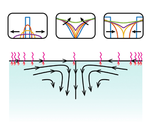
For sufficiently elongated surfactant distributions (e.g. a ‘strip’ of surfactant) and a sufficiently deep fluid subphase, the problem can be reduced to the unbounded, two-dimensional scenario displayed in figure 1. We use a coordinate system where $x$ spans the interface and $y$ points away from the fluid subphase, with $\boldsymbol {e}_x$ and $\boldsymbol {e}_y$ the unit vectors in the $x$ and $y$ directions, respectively. Velocity components are denoted $u$ and $v$, with $\boldsymbol {u}=u\boldsymbol {e}_x+v\boldsymbol {e}_y$. The domain is considered to be semi-infinite, defined in $x\in (-\infty,\infty )$ and $y\in (-\infty,0]$, and the time evolution of the surfactant concentration $\varGamma (x,t)$ along the interface is given by

(2.3)\begin{equation} \dfrac{\partial^{}\varGamma}{\partial t^{}} + \dfrac{\partial^{}(u_s\varGamma)}{\partial x^{}} = D_s\dfrac{\partial^{2}\varGamma}{\partial x^{2}}, \end{equation}

where $D_s$ is the surface diffusivity of the surfactant and $u_s = \boldsymbol {u}\boldsymbol {\cdot }\boldsymbol {e}_x|_{y=0}$ is the interfacial velocity. The boundary conditions at the interface

(2.4a)$$\begin{gather} \left.\boldsymbol{e}_x\boldsymbol{\cdot}\boldsymbol{\sigma}\boldsymbol{\cdot}\boldsymbol{e}_y\right|_{y=0} = {-}a\dfrac{\partial^{}\varGamma}{\partial x^{}}, \end{gather}$$

(2.4b)$$\begin{gather}v(y=0) = 0, \end{gather}$$

are the Marangoni condition (2.4a) linking viscous stresses to the gradient of surfactant, and the no-penetration kinematic condition (2.4b). Here, the parameter

(2.5)\begin{equation} {a =\left|\dfrac{\,\mathrm{d}^{}\gamma}{\,\mathrm{d}\varGamma^{}}\right|}, \end{equation}

is a normalized Marangoni modulus, quantifying the reduction of surface tension $\gamma$ with increasing surfactant concentration. We regard $D_s$ and $a$ as constants, although they are in general dependent on $\varGamma$ through equations of state $D_s(\varGamma )$ and $\gamma (\varGamma )$, e.g. see Manikantan & Squires (Reference Manikantan and Squires2020).

Figure 1. A non-homogeneous distribution of insoluble surfactant, with concentration $\varGamma (x,t)$, induces a velocity field $\boldsymbol {u}(\boldsymbol {x},t)$ within its fluid subphase through interfacial Marangoni stresses. The surfactant is itself advected by the resulting interfacial velocity $u_s(x,t)=\boldsymbol {u}\boldsymbol {\cdot }\boldsymbol {e}_x|_{y=0}$, leading to a two-way coupled problem. (a) For a localized pulse of surfactant, the Marangoni flow results in outward ‘spreading’. (b) When the surfactant distribution is instead depleted at its centre (a ‘hole’ or a ‘dimple’), the result is an inward ‘filling’ flow. All the dimensional parameters of the model considered here are highlighted in panel (b).

The governing equations (2.2)–(2.3) and boundary conditions (2.4) are supplemented with an initial condition for the surfactant distribution

(2.6)\begin{equation} \varGamma(x,t=0) = \varGamma_0(x). \end{equation}

The profile $\varGamma _0(x)$ introduces the characteristic scale $\varGamma _c$, which we will take as the maximum concentration $\varGamma _c = \max _x{[\varGamma _0(x)]}$. Furthermore, the typical width of $\varGamma _0(x)$ sets the length scale $l_c$ of the problem.

From these constants, dimensional analysis of the Marangoni boundary condition (2.4a) leads to a natural scale for the velocity magnitude

(2.7)\begin{equation} \left.\boldsymbol{e}_x\boldsymbol{\cdot}\boldsymbol{\sigma}\boldsymbol{\cdot}\boldsymbol{e}_y\right|_{y=0} = \left.\mu\dfrac{\partial^{}u}{\partial y^{}}\right|_{y=0} = {-}a\dfrac{\partial^{}\varGamma}{\partial x^{}} \implies u_c \approx \dfrac{a\varGamma_c}{\mu}. \end{equation}

For the assumptions of $Re\ll {1}$ and $Ca\ll {1}$ to hold, the characteristic concentration $\varGamma _c$ and width $l_c$ of the surfactant distribution must both be sufficiently small to ensure that

(2.8)\begin{equation} l_c\varGamma_c \ll \dfrac{\mu^2}{\rho{a}}, \quad \varGamma_c \ll \dfrac{\gamma_0}{a}, \end{equation}

providing practical estimates to determine if, for a given set of physicochemical properties $\mu$, $\rho$, $a$, and $\gamma _0$, a known surfactant distribution will lead to Marangoni flow in the asymptotic limit considered in this study.

The full problem, as defined by (2.2)–(2.4) and (2.6), is nonlinear and involves the two-dimensional vector field $\boldsymbol {u}$. Thess et al. (Reference Thess, Spirn and Jüttner1995) recognized that it was possible to obtain a one-dimensional formulation, using the Fourier transform of (2.2) to obtain $u_s$ as a function of $\varGamma$. Here, we show that the same simplification can be achieved through the boundary integral representation of Stokes flow. Indeed, the velocity field given by (2.2) at any position $\boldsymbol {x}$ along the interface (see Pozrikidis Reference Pozrikidis1992) can be expressed as

(2.9)\begin{equation} {\boldsymbol{u}(\boldsymbol{x},t) = \dfrac{1}{2{\rm \pi}}\left[\int_\mathcal{I}\boldsymbol{\mathsf{G}}(\boldsymbol{x}-\boldsymbol{x}')\boldsymbol{\cdot}\boldsymbol{\sigma}(\boldsymbol{x}',t)\boldsymbol{\cdot}\boldsymbol{n}\,\mathrm{d}{l_{\boldsymbol{x}'}}+{\int\hskip -1,05em -\,}_\mathcal{I}\boldsymbol{u}(\boldsymbol{x}',t)\boldsymbol{\cdot}\boldsymbol{\mathsf{T}}(\boldsymbol{x}-\boldsymbol{x}')\boldsymbol{\cdot}\boldsymbol{n}\,\mathrm{d}{l_{\boldsymbol{x}'}}\right]}, \end{equation}

where the dash denotes the Cauchy principal value of the integral, $\mathcal {I}$ denotes the interface, $\boldsymbol {n}$ the unit outward normal vector and the tensors in the integrands are defined as

(2.10a)$$\begin{gather} \boldsymbol{\mathsf{G}}(\boldsymbol{x}) ={-}\dfrac{1}{\mu}\left(\ln|\boldsymbol{x}|\,\boldsymbol{\mathsf{I}}-\dfrac{\boldsymbol{x}\boldsymbol{x}}{|\boldsymbol{x}|^2}\right), \end{gather}$$

(2.10b)$$\begin{gather}\boldsymbol{\mathsf{T}}(\boldsymbol{x}) ={-}4\dfrac{\boldsymbol{x}\boldsymbol{x}\boldsymbol{x}}{|\boldsymbol{x}|^4}. \end{gather}$$

Since the interface remains flat, the outward normal vector simplifies as $\boldsymbol {n}=\boldsymbol {e}_y$, while $\boldsymbol {x}$ and $\boldsymbol {x}'$ are co-linear and parallel to $\boldsymbol {e}_x$. Therefore, we have $(\boldsymbol {x}-\boldsymbol {x}')\boldsymbol {\cdot }\boldsymbol {n}=0$ since the vectors are orthogonal, and

(2.11)\begin{equation} \boldsymbol{\mathsf{T}}(\boldsymbol{x}-\boldsymbol{x}')\boldsymbol{\cdot}\boldsymbol{n} ={-}4\dfrac{(\boldsymbol{x}-\boldsymbol{x}')(\boldsymbol{x}-\boldsymbol{x}')(\boldsymbol{x}-\boldsymbol{x}')}{|\boldsymbol{x}-\boldsymbol{x}'|^4}\boldsymbol{\cdot}\boldsymbol{n} = \boldsymbol{\mathsf{0}}, \end{equation}

eliminating the second integral (the ‘double-layer potential’) in (2.9). Taking $(\boldsymbol {x}-\boldsymbol {x}')=(x-x')\boldsymbol {e}_x$ and noting the integrals along the interface are simply along $x'$, the interfacial velocity can then be expressed as

(2.12)\begin{equation} u_s(x,t) = \left.\boldsymbol{e}_x\boldsymbol{\cdot}\boldsymbol{u}\right|_{y=0} = \dfrac{1}{2{\rm \pi}\mu}\int_{-\infty}^{\infty}\left(1-\ln|x-x'|\right)\left.\boldsymbol{e}_x\boldsymbol{\cdot}\boldsymbol{\sigma}(x',t)\boldsymbol{\cdot}\boldsymbol{e}_y\right|_{y=0}\,\mathrm{d}\kern 0.06em {x'}, \end{equation}

which, upon substitution of the Marangoni boundary condition (2.4a) and integration by parts, becomes

(2.13)\begin{equation} u_s(x,t) = \dfrac{a}{2{\rm \pi}\mu}\left\{\left[\left(\ln|x-x'|-1\right)\varGamma(x',t)\right]_{x'\to-\infty}^{x'\to\infty} +{\int\hskip -1,05em -\,}_{-\infty}^{\infty}\dfrac{\varGamma(x',t)}{x-x'}\,\mathrm{d}\kern 0.06em {x'}\right\}. \end{equation}

The first term in (2.13) vanishes for any surfactant profile decaying as a power law (or faster) in the far field. Remarkably, this term also cancels out for profiles $\varGamma (x,t)$ that do not decay as $|x|\to \infty$, as long as their far-field values are finite and symmetric, such that $0<\lim _{x\to \infty }\varGamma (x,t) = \lim _{x\to -\infty }\varGamma (x,t)<\infty$. We therefore restrict this study to these two possible far-field behaviours, excluding ‘step-like’ profiles with asymmetric far-field concentrations. The above leads to the closure relationship

(2.14)\begin{equation} u_s(x,t) = \dfrac{a}{2{\rm \pi}\mu}{\int\hskip -1,05em -\,}_{-\infty}^{\infty}\dfrac{\varGamma(x',t)}{x-x'}\,\mathrm{d}\kern 0.06em {x'} = \dfrac{a}{2\mu}\mathcal{H}[\varGamma], \end{equation}

first derived by Thess et al. (Reference Thess, Spirn and Jüttner1995), where the operator $\mathcal {H}\left [\ \right ]$ denotes the Hilbert transform of a function (for details, see King Reference King2009a,Reference Kingb). This closure relationship results in a one-dimensional problem, only requiring the solution of (2.3) alongside condition (2.14). The resulting formulation is, however, non-local, as the interfacial velocity $u_s$ at any given point depends upon the distribution of $\varGamma$ along the whole real line.

We proceed to non-dimensionalize equations (2.3), (2.14) and the initial condition (2.6) using the scales of the problem discussed above. To that end, we apply the rescalings

(2.15)\begin{equation} x \to l_c{x}, \quad t \to \left(\dfrac{2\mu{l_c}}{a\varGamma_c}\right)t, \quad u \to \left(\dfrac{a\varGamma_c}{2\mu}\right)u, \quad \varGamma \to \varGamma_c\varGamma, \quad \varGamma_0 \to \varGamma_c\varGamma_0, \end{equation}

which leads to a dimensionless problem given by

(2.16a)$$\begin{gather} \dfrac{\partial^{}\varGamma}{\partial t^{}} + \dfrac{\partial^{}(\mathcal{H}\left[\varGamma\right]\varGamma)}{\partial x^{}} = \dfrac{1}{Pe_s}\dfrac{\partial^{2}\varGamma}{\partial x^{2}}, \end{gather}$$

(2.16b)$$\begin{gather}\varGamma(x,t=0) = \varGamma_0(x), \end{gather}$$

and where the surface Péclet number is defined as

(2.17)\begin{equation} Pe_s := \dfrac{a\varGamma_cl_c}{2\mu{D_s}}. \end{equation}

Alternative formulations of the non-local problem (2.16) have been studied in the mathematical literature (Baker et al. Reference Baker, Li and Morlet1996; Morlet Reference Morlet1998; Chae et al. Reference Chae, Córdoba, Córdoba and Fontelos2005; de la Hoz & Fontelos Reference de la Hoz and Fontelos2008; Eggers & Fontelos Reference Eggers and Fontelos2020) as a model for finite-time blowup. However, that body of work was not concerned with the description of surfactant dynamics, which introduces key differences that we highlight in § 2.3 below. In the context of Marangoni flows, Crowdy (Reference Crowdy2021b) recently showed, through a complex-variable formulation of two-dimensional Stokes flow, that a dependent variable $\psi =u_s+\mathrm {i}\varGamma = \mathcal {H}\left [\varGamma \right ] + \mathrm {i}\varGamma$ satisfies

(2.18a)$$\begin{gather} \dfrac{\partial^{}\psi}{\partial t^{}} + \psi\dfrac{\partial^{}\psi}{\partial x^{}} = \dfrac{1}{Pe_s}\dfrac{\partial^{2}\psi}{\partial x^{2}}, \end{gather}$$

(2.18b)$$\begin{gather}\psi(x,t=0) = \psi_0(x) = {\mathcal{H}\left[\varGamma_0(x)\right]+\mathrm{i}\varGamma_0(x)}, \end{gather}$$

where $\psi (z,t)$ must be a lower-analytic complex function (named $h(z,t)$ in the notation of Crowdy Reference Crowdy2021b) of the variable $z=x+\mathrm {i}{y}$. This problem reduction can also be realized by adding (2.16a) to its Hilbert transform, and then recognizing that $\mathcal {H}\left [\partial _x\varGamma \right ]=\partial _x\mathcal {H}\left [\varGamma \right ]$ and $\mathcal {H}\left [\varGamma \mathcal {H}\left [\varGamma \right ]\right ]=((\mathcal {H}\left [\varGamma \right ])^2-\varGamma ^2)/2$. It is worth remarking that subtracting (2.16a) from its Hilbert transform leads to the same Burgers equation (2.18a) but with a complex conjugate dependent variable $\psi =u_s-\mathrm {i}\varGamma$, which is an equivalent notation followed by Bickel & Detcheverry (Reference Bickel and Detcheverry2022). In such an alternative notation the complex function $\psi (z,t)$ is instead the upper-analytic Schwarz conjugate of the one used here.

The limit of negligible diffusion given by $Pe_s\gg {1}$ can be approximated at leading order by taking $Pe_s^{-1}=0$, which yields

(2.19a)$$\begin{gather} \dfrac{\partial^{}\psi}{\partial t^{}} + \psi\dfrac{\partial^{}\psi}{\partial x^{}} = 0, \end{gather}$$

(2.19b)$$\begin{gather}\psi(x,t=0) = \psi_0(x) = {\mathcal{H}\left[\varGamma_0(x)\right]+\mathrm{i}\varGamma_0(x)}. \end{gather}$$

The problems given by the Burgers equation (2.18a) and the inviscid Burgers equation (2.19a) (also known as the Hopf equation) are now local, and admit exact solutions via either the Cole–Hopf transformation for (2.18) or the method of characteristics for (2.19), as shown in Crowdy (Reference Crowdy2021b) and Bickel & Detcheverry (Reference Bickel and Detcheverry2022). While some of these solutions have been shown to exhibit self-similar behaviour (Thess Reference Thess1996; Bickel & Detcheverry Reference Bickel and Detcheverry2022), a systematic analysis of the problem from the perspective of self-similarity has not yet been performed, and is the goal of this paper.

2.2. Self-similar formulation

We adopt the following self-similarity ansatzes:

(2.20a)$$\begin{gather} \eta = \mathrm{sgn}\left(t-t_*\right)\dfrac{x-x_*}{A|t-t_*|^\beta}, \end{gather}$$

(2.20b)$$\begin{gather}\psi(x,t) = {B}|t-t_*|^\alpha f(\eta), \end{gather}$$

with $\eta$ the real similarity variable. The similarity function $f(\eta )$, which takes complex values, is decomposed as ${f = U + \mathrm {i}C}$, with $U(\eta )$ and $C(\eta )$ real. The interfacial velocity and surfactant concentration can then be recovered as

(2.21a)$$\begin{gather} u_s(x,t) = {B} |t-t_*|^{\alpha} U(\eta), \end{gather}$$

(2.21b)$$\begin{gather}\varGamma(x,t) = {B} |t-t_*|^{\alpha} C(\eta). \end{gather}$$

We introduce the positive real constants $A$ and $B$ for convenience, and fix their values to simplify the final form of the similarity solutions $f(\eta )$, as illustrated below. The real constants $x_*$ and $t_*$ are a reference position and time, respectively. Including the factor $\mathrm {sgn}\left (t-t_*\right )$ in the definition (2.20a) is equivalent to choosing

(2.22a)\begin{equation} \eta =\dfrac{x-x_*}{A(t-t_*)^\beta}, \end{equation}

for solutions that evolve forward in time $t>t_*$, and to choosing

(2.22b)\begin{equation} \eta =\dfrac{x_*-x}{A(t_*-t)^\beta}, \end{equation}

for solutions that evolve backward in time $t< t_*$. We adopt the more intuitive forward-time description when describing ‘spreading’ (as in figure 1a) solutions of (2.18) and (2.19). These solutions become self-similar at long times $t\gg {1}$, so in that case we take $t_*=0$. However, ‘filling’ self-similar solutions representing inward flow (as in figure 1b) are often only valid sufficiently close to a reference time $t=t_*>0$ at which the solution has a singularity, requiring either the backward-time (e.g. Eggers & Fontelos Reference Eggers and Fontelos2008) or the forward-time (e.g. Zheng et al. Reference Zheng, Fontelos, Shin and Stone2018) description to analyse their behaviour immediately prior or subsequent to $t_*$, respectively.

Using the self-similarity ansatzes (2.20) in the Burgers equation (2.18a) leads to

(2.23)\begin{equation} \alpha{f}-\beta\eta\dfrac{\,\mathrm{d}^{}f}{\,\mathrm{d}\eta^{}} + {\dfrac{B}{A}}|t-t_*|^{\alpha-\beta+1}f\dfrac{\,\mathrm{d}^{}f}{\,\mathrm{d}\eta^{}} = \dfrac{\mathrm{sgn}\left(t-t_*\right)}{A^2Pe_s}|t-t_*|^{1-2\beta}\dfrac{\,\mathrm{d}^{2}f}{\,\mathrm{d}\eta^{2}}. \end{equation}

Solutions are self-similar when the above ordinary differential equation (ODE) is solely dependent on $\eta$, and not on $t$ or $x$ separately, which requires either one of the following two scenarios:

1. (i) For the general case of a finite $Pe_s^{-1}>0$, the only possible choice of exponents is $\alpha =-1/2$, $\beta =1/2$. Seeking to eliminate parameters from (2.23), we fix $A=B=\sqrt {2/Pe_s}$, focusing on forward-time solutions with $\mathrm {sgn}\left (t-t_*\right )=1$ that lead to

   (2.24)\begin{equation} \dfrac{\,\mathrm{d}^{}}{\,\mathrm{d}\eta^{}}\left[\dfrac{\,\mathrm{d}^{}f}{\,\mathrm{d}\eta^{}}+\eta{f}-f^2\right]=0. \end{equation}
   Equation (2.24) has one spreading (as in figure 1a) self-similar solution of the first kind, which was identified by Bickel & Detcheverry (Reference Bickel and Detcheverry2022) and which we outline in § 4.2.

2. (ii) In the advection-dominated limit given by $Pe_s^{-1}=0$, self-similarity only requires $\alpha =\beta -1$. In this case, we fix $B=A$, keeping $\beta$ and $A$ as free parameters. This leads to

   (2.25)\begin{equation} (f-\beta\eta)\dfrac{\,\mathrm{d}^{}f}{\,\mathrm{d}\eta^{}} = (1-\beta){f}. \end{equation}
   We obtain the same similarity equation (2.25) independently of the choice of the forward-time or backward-time definition of $\eta$, due to the invariance of the inviscid Burgers equation (2.19a) with respect to a reversal of time $t\to {-t}$ and space $x\to {-x}$. In this advection-dominated case, multiple solutions can potentially arise, depending on the specific value of $\beta$. Using a phase-plane formalism and stability analysis, in § 3 we identify five possible similarity solutions of (2.25). We re-discover the spreading self-similar solution of the first kind first identified by Thess (Reference Thess1996), which we detail in § 4.1. We also find four possible ‘filling’ (as in figure 1b) solutions of the second kind with different power-law exponents $\beta$, which we describe in § 5.

For either of the two similarity differential equations (2.24) and (2.25) above, solutions $f(\eta )$ must have a physically correct parity. Introducing the similarity ansatzes (2.20) into the closure relationship $u_s(x,t)=\mathcal {H}\left [\varGamma (x,t)\right ]$ leads to an analogous relation $U(\eta )=\mathcal {H}\left [C(\eta )\right ]$ for the similarity solutions. Since the Hilbert transform reverses parity (King Reference King2009a), we can conclude that the only admissible parities are either $U$ odd and $C$ even, or $U$ even and $C$ odd. However, an odd function $C(\eta )$ would imply unphysical negative values of the concentration $\varGamma (x,t)$. Accordingly, we only consider similarity solutions with $U(\eta )$ odd and $C(\eta )$ even or, equivalently, $f(-\eta )=-\overline {f(\eta )}$ with the overbar indicating complex conjugation. Note that this parity requirement does not necessarily apply to the physical solutions $\varGamma (x,t)$ and $u_s(x,t)$ which, as we show in §§ 4 and 5, can be asymmetric and only attain symmetry as they converge to a self-similar solution.

In addition, similarity solutions $f(\eta )$ must satisfy a specific far-field boundary condition (Eggers & Fontelos Reference Eggers and Fontelos2008) such that the function $\psi (x,t)$ is independent of time in the far field $|x|\to \infty$. From the similarity ansatz (2.20b) and from the fact that $\alpha =\beta -1$, it is clear that such a far-field behaviour requires $f(\eta ) =O(|t-t_*|^{1-\beta })$ as $|\eta |\to \infty$. Given the definition of $\eta$ in (2.20a), the only possibility to satisfy this condition is

(2.26)\begin{equation} f(\eta) \sim {k_{{\pm}\infty}} |\eta|^{({\beta-1})/{\beta}} \quad\text{as }|\eta|\to\infty. \end{equation}

We use the notation ${k_{\pm \infty }}$ to denote generic far-field constants that differ between ${k_{\infty }}$ as $\eta \to \infty$ and ${k_{-\infty }}$ as $\eta \to -\infty$ since, by symmetry, ${k_{-\infty }=-\bar {k}_{\infty }}$. Equation (2.26) is referred to as a ‘quasi-stationary’ far-field condition. If the similarity solution $f(\eta )$ is globally valid in space, then the condition is equivalent to a far-field behaviour of $\psi$ that is constant in time as $|x|\to \infty$. If, on the other hand, $f(\eta )$ is only valid locally (as is often the case with similarity of the second kind), the condition implies that $f(\eta )$ must match with the ‘outer’ non-self-similar part of $\psi$, which evolves on a slower time scale.

2.3. A note on alternative formulations

The problem given by (2.16) and (2.18), as well as its variants with $Pe_s^{-1}=0$, appear in the literature with slightly different formulations that are nonetheless equivalent, which we summarize in table 1. It is easy to check that, once transformed to our formulation, the finite-time blowup described in the mathematical literature (Baker et al. Reference Baker, Li and Morlet1996; Morlet Reference Morlet1998; Chae et al. Reference Chae, Córdoba, Córdoba and Fontelos2005; de la Hoz & Fontelos Reference de la Hoz and Fontelos2008; Eggers & Fontelos Reference Eggers and Fontelos2020) occurs for negative concentration $\varGamma <0$. This is unphysical if $\varGamma$ represents a surfactant concentration, but it is not problematic in the above body of work, where the non-local problem (2.16) has an unrelated physical motivation. Those studies describe singularities that are persistent in time and occur at points with $\varGamma <0$, thus qualitatively different from those found here (§ 5), which happen at points of $\varGamma =0$ within a non-negative profile $\varGamma (x)\geq {0}$, and disappear at finite time. For that reason, the self-similar analysis by de la Hoz & Fontelos (Reference de la Hoz and Fontelos2008) and Eggers & Fontelos (Reference Eggers and Fontelos2020) is linearized around the non-zero value of $\varGamma$ at which singularities occur, yielding different similarity equations and exponents.

Table 1. Alternative formulations of the problem found in the literature, alongside the transformations required to convert them to (2.16), (2.18) and their variants with $Pe_s^{-1}=0$. Here, we have that $\tilde {\mathcal {H}}\left [\varGamma \right ] = {\rm \pi}^{-1}{\int\hskip -1,05em -\,} _{-\infty }^\infty (x'-x)^{-1}\varGamma (x',t)\,\,\mathrm {d}\kern 0.06em {x'}$ is an alternative definition of the Hilbert transform, such that $\tilde {\mathcal {H}}\left [\varGamma \right ]=-\mathcal {H}\left [\varGamma \right ]$. Subindices indicate partial derivatives.

3.1. The phase plane

Since (3.1) is also autonomous, its solutions can be represented in a phase plane with state variables $\mathrm {Re}\left [g\right ]=U/\eta$ and ${\mathrm {Im}\left [g\right ]=C/\eta }$, following Gratton & Minotti (Reference Gratton and Minotti1990). This formalism allows systematic identification of all possible similarity solutions of (2.25) as distinct trajectories in the phase plane, with the beginning of each trajectory representing the origin $\eta =0$ and its end point indicating the far field $|\eta |\to \infty$. We construct the phase plane by first finding the fixed points of (3.1), seeding initial conditions closely around each of them, and then numerically integrating forward or backward in $\ln |\eta |$ depending on if the particular seed is along a stable or unstable direction. A detailed account of the integration procedure and the calculation of the fixed points is provided in Appendix A. We only consider exponents $\beta >0$, excluding also $\beta =1$ since it leads to a linear problem in (3.1) with constant solutions for $f(\eta )$.

Phase portraits of the system are shown in figure 2, for a set of six representative values of $\beta$. The phase plane has a remarkably simple structure, being symmetric with respect to the horizontal axis $C/\eta =0$ due to the invariance of (3.1) to $g\to \bar {g}$. Note that the symmetry $f(-\eta )=-\overline {f(\eta )}$ required of the similarity solution leads to $g(-\eta )=\overline {g(\eta )}$, given that $f(\eta )=\eta \,{g}(\eta )$. In the phase plane, this means that a full solution is represented by a combination of a trajectory in the upper half-plane (given by $g$) and its reflection in the lower half-plane (given by $\bar {g}$). The curve in the upper half-plane (where $C(\eta )/\eta >0$) represents the solution for $\eta >0$ (since $C(\eta )$ must be non-negative), while its mirror image in the lower half-plane (where $C(\eta )/\eta <0$) represents it for $\eta <0$.

Figure 2. Phase portraits of (3.1), for six different values of $\beta >0$, $\beta \neq {1}$. Any given two trajectories that are symmetric with respect to the horizontal axis represent one possible similarity solution $f(\eta )=\eta \,{g(\eta )}$, with the origin of the trajectory denoting $\eta =0$ and the endpoint denoting $|\eta |\to \infty$. The three fixed points $O=(0,0)$ (stable node), $P=(1,0)$ (node) and $S=(\beta,0)$ (saddle) have horizontal and vertical eigendirections for all $\beta >0$. Points $M$, $N$, $R$ are the fixed points of the ODE satisfied by the reciprocals of the solution (see Appendix A). Only green, purple, orange and yellow trajectories represent similarity solutions that are physically relevant, as illustrated in table 3. Stability criteria (§ 3.2) select the only five solutions that can be obtained in practice, which are highlighted with a wider streak. The dashed vertical line corresponds to $U/\eta =1-\beta$.

The fixed points of the phase plane always include two star nodes $O=(0,0)$ and $P=(1,0)$ on the horizontal axis, whose position is independent of the value of the exponent $\beta$. In addition, there is always a saddle point $S=(\beta,0)$ that lies between $O$ and $P$ for $0<\beta <1$ and to the right of $P$ for $\beta >1$, denoting a ‘front’ where the solution is locally non-smooth. These three points $O$, $P$, and $S$ have horizontal and vertical eigendirections. The behaviour of trajectories at the outer edges of the phase plane (i.e. as $U/\eta \to \pm \infty$ or as $C/\eta \to \pm \infty$) is given by three additional fixed points (labelled $M$, $N$ and $R$) that the ODE (3.1) displays when it is recast in terms of the reciprocals $\eta /U$ and $\eta /C$, as detailed in Appendix A. All six fixed points are listed and classified in table 2. Furthermore, the asymptotic form of the solution around each of these points can be found via linearization and is also provided in table 2, thereby listing all possible behaviours of $f(\eta )$ as $\eta \to 0$ and as $|\eta |\to \infty$ for different values of $\beta$. The fact that two trajectories (one representing $\eta >0$ and another one $\eta <0$) must be ‘patched’ at $\eta =0$ to generate a full solution $f(\eta )$ results in expansions around the origin that often involve terms like $\mathrm {sgn}\left (\eta \right )$ and $|\eta |$ (see table 2), which can only result in regular solutions for some specific values of $\beta$, as we show in § 3.2.

Table 2. Fixed points of the ODE system given by the real and imaginary parts of (3.1), for $\beta >0$ and $\beta \neq {1}$; SN denotes a stable node, UN an unstable node, and S a saddle. Points $M$, $N$ and $R$ are obtained as fixed points of ODE systems involving the reciprocals $\eta /U$ and $\eta /C$, as detailed in Appendix A. The entries for $U(\eta )$ and $C(\eta )$ denote every possible asymptotic expansion about each fixed point, where $K$ and $K'$ are independent, real, non-zero constants of integration, and $\eta _f$ is the (real, non-zero) location of the front occurring at the saddle point $S$. When more than one entry for $U(\eta )$ and $C(\eta )$ is provided, the first row corresponds to the trajectory along the horizontal eigendirection, the second row to the trajectory along the vertical eigendirection and the third (if provided) to generic curves along any other direction.

While all possible similarity solutions with the correct parity can be placed in the plane, not all of them are necessarily relevant from a physical standpoint. The advantage of a phase plane formalism is that it provides a way to systematically classify all trajectories in terms of the fixed points that they connect, so that they can be identified as relevant or irrelevant. We list all possible trajectories in table 3, where the rightmost column indicates whether the trajectory is classified as physically relevant, based on three criteria:

1. (i) Solutions must be representative of Marangoni flow. Some trajectories in figure 2 like $M\to {O}$, $M\to {P}$ or $P\to {O}$ are fully contained along the horizontal axis, but that implies a zero concentration $C(\eta )=0$ for all values of $\eta$, indicating that they do not represent Marangoni flow. In fact, the trajectory $P\to {O}$ along the horizontal axis for $\beta =3/2$ (figure 2d) corresponds to the real similarity solution of the inviscid Burgers equation (2.19a) described by Eggers & Fontelos (Reference Eggers and Fontelos2008), which appears prior to the formation of a shock and is relevant to describe other problems like gas dynamics or wave breaking.

2. (ii) Solutions must have a far-field behaviour compatible with (2.26), as explained in § 2.2. Accordingly, all trajectories listed in table 2 with a far field incompatible with (2.26), such as those ending at point $P$ for $0<\beta <1$, are labelled as irrelevant.

3. (iii) Solutions must be continuous at the origin. For instance, solutions starting at points $M$ or $R$ have an odd but discontinuous velocity $U(\eta )$ at $\eta =0$, with $U(0^+)=K$ and $U(0^-)=-K$ for some real, non-zero constant $K$, as detailed in table 2.

Table 3. List of all possible phase-plane trajectories of the reduced similarity ODE (3.1), for different values of the exponent $\beta$. The last column indicates whether a given trajectory represents a physically relevant solution. If the solution is classified as not relevant, the reasons are provided, based on three criteria: (i) having a non-zero concentration $C(\eta )\neq {0}$ representative of Marangoni flow, (ii) compatibility with the far-field condition (2.26) and (iii) continuity at $\eta =0$. If the trajectory is physically relevant, its colour in figure 2 is indicated.

Based on this classification outlined in table 3, we identify four families of solutions that qualify as physically relevant. We can interpret the qualitative behaviour of each of these trajectories depending on their position within the phase plane, following the discussion given in Appendix B. Trajectory $N\to {S}\to {O}$, which only exists for $\beta =1/2$, is highlighted in green in figure 2 and, according to Appendix B, corresponds to a ‘spreading’ similarity solution with a forward-time definition of the similarity variable, as in (2.22a). We discuss this spreading solution, as well as its counterpart with finite diffusion, in § 4. The $P\to {O}$ (yellow in figure 2) and $P\to {S}\to {O}$ (orange in figure 2) trajectories are ‘filling’ similarity solutions with a backward-time scaling as in (2.22b), which suggests they are valid immediately prior to a singularity. They only hold locally as evidenced by their far-field behaviour, since these solutions only exist for $\beta >1$ and the condition (2.26), $f(\eta )\sim {k_{\pm \infty }}|\eta |^{({\beta -1})/{\beta }}$, then implies that they grow unbounded as $|\eta |\to \infty$. The Hilbert transform is undefined for unbounded functions so, as observed by Thess et al. (Reference Thess, Spirn and Jüttner1997), similarity solutions for $\beta >1$ must be only valid locally. The last of these four families of solutions is $N\to {O}$, which exists for $\beta >1/2$, is displayed in purple in figure 2 and has forward-time scaling as in (2.22a). These solutions can be either spreading, for $1/2<\beta <1$, or filling, for $\beta >1$.

Three of the identified families of curves, namely $P\to {O}$ (yellow), $P\to {S}\to {O}$ (orange) and $N\to {O}$ (purple), appear to exist for multiple values of $\beta$, which is typical of self-similarity of the second kind (Barenblatt Reference Barenblatt1996). In the case of $P\to {O}$, there are even several possible solutions within the same value of $\beta$. These second-kind solutions appear around finite-time singularities, and we show in § 3.2 how considerations about their stability rule out many of the trajectories within these three families, leading to the only solutions that are truly obtainable in practice.

3.2. Stability analysis

In order to analyse the stability of similarity solutions, we use the dynamical system formulation (see Giga & Kohn Reference Giga and Kohn1985, Reference Giga and Kohn1987; Eggers & Fontelos Reference Eggers and Fontelos2008, Reference Eggers and Fontelos2015) of the inviscid Burgers equation (2.19a). Instead of seeking to reduce the two physical variables $x$ and $t$ into a single similarity variable $\eta$, we use the more general change of variables

(3.4a)$$\begin{gather} \psi(x,t) = A|t-t_*|^{\beta-1}F(\eta,\tau), \end{gather}$$

(3.4b)$$\begin{gather}\eta = \mathrm{sgn}\left(t-t_*\right)\dfrac{x-x_*}{A|t-t_*|^\beta}, \end{gather}$$

(3.4c)$$\begin{gather}\tau ={-}\ln{|t-t_*|}, \end{gather}$$

which, instead of reducing the original partial differential equation (PDE) to an ODE, leads to a partial differential equation for $F(\eta,\tau )$

(3.5)\begin{equation} \dfrac{\partial^{}F}{\partial\tau^{}} = \left[(F-\beta\eta)\dfrac{\partial^{}F}{\partial\eta^{}} - (1-\beta)F\right]. \end{equation}

The key of the transformation given by (3.4) is that the steady state of (3.5) reduces to the similarity equation (2.25). Indeed, the definition (3.4c) of $\tau$ indicates that approaching the singularity time $t\to {t}_*$ corresponds to $\tau \to \infty$, leading to a steady state $\partial _\tau {F}\to {0}$ at which solutions to (3.5) satisfy the similarity ODE (2.25).

The stability of each of the similarity solutions found in § 3.1 can now be determined via linear stability analysis around $f(\eta )$. We pose a perturbation

(3.6)\begin{equation} F(\eta,\tau) = f(\eta) + \varepsilon\sum_{n=0}^{\infty}b_n{\rm e}^{\nu_n\tau}\phi_n(\eta) + O(\varepsilon^2), \end{equation}

where $\varepsilon \ll {1}$, $\nu _n$ are the growth rates of each mode $\phi _n$ and $b_n$ are the mode amplitudes. Introducing (3.6) into the PDE (3.5) we obtain at order $O(\varepsilon )$ an eigenvalue problem

(3.7)\begin{equation} \mathcal{L}\phi_n := \left[\dfrac{\beta(1-\beta)}{(f-\beta\eta)}\eta+(f-\beta\eta)\dfrac{\,\mathrm{d}^{}}{\,\mathrm{d}\eta^{}}\right]\phi_n = \nu_n\phi_n. \end{equation}

The stability of any given similarity solution $f(\eta )$ can then be determined solving the eigenvalue problem (3.7) for the linear operator $\mathcal {L}$, which itself depends on the similarity solution $f(\eta )$. Moreover, the spectrum of $\mathcal {L}$ is typically discrete given some additional conditions for the eigenfunctions $\phi _n$ (Eggers & Fontelos Reference Eggers and Fontelos2008, Reference Eggers and Fontelos2015). Namely, each $\phi _n(\eta )$ must be regular at $\eta =0$, and satisfy its own quasi-stationary far-field condition

(3.8)\begin{equation} \phi_n(\eta) \sim {k_{{\pm}\infty}} |\eta|^{({\beta-1-\nu_n})/{\beta}} \quad \text{as } |\eta|\to\infty, \end{equation}

for some complex constants $k_{\pm \infty }$. Only those similarity solutions leading to a spectrum of $\mathcal {L}$ with negative eigenvalues $\nu _n<0$ result in perturbations decaying in time and are therefore stable. However, as shown by Eggers & Fontelos (Reference Eggers and Fontelos2008, Reference Eggers and Fontelos2015), there is also a specific subset of non-negative eigenvalues that does not lead to instability and is instead an artefact of the continuous symmetries of the problem. Specifically, the invariance of the governing equation (2.19a) to shifts in space $x\to {x}+\lambda$, shifts in time $t\to {t}+\lambda$ and scalings $\psi \to \lambda \psi$, $t\to \lambda {t}$, $x\to \lambda ^2x$, always leads to the three eigenvalues $\nu =\beta$, $\nu =1$ and $\nu =0$, respectively (see § 3.2 in Eggers & Fontelos Reference Eggers and Fontelos2015). Accordingly, we look for solutions from the phase plane that lead to a spectrum of $\mathcal {L}$ with at most these three non-negative eigenvalues, with all others being negative.

The three families of trajectories in figure 2 considered here ($P\to {O}$, $P\to {S}\to {O}$ and $N\to {O}$) all have the same far-field behaviour since they end at the same point. From table 2, we know that $f(\eta )\sim {k_{\pm \infty }}|\eta |^{({\beta -1})/{\beta }}$ as $|\eta |\to \infty$, which can be introduced in the eigenvalue problem (3.7) to yield the far-field behaviour of the eigenfunctions

(3.9)\begin{equation} \dfrac{\,\mathrm{d}^{}\phi_{n}}{\,\mathrm{d}\eta^{}} = \left[\dfrac{\nu_{n}(f-\beta\eta)-\beta(1-\beta)\eta}{(f-\beta\eta)^2}\right]\phi_{n} \sim\left[\dfrac{\beta-1-\nu_n}{\beta\eta}\right]\phi_n \quad\text{as }|\eta|\to\infty, \end{equation}

which leads to $\phi _n\sim {k_{\pm \infty }}|\eta |^{({\beta -1-\nu _n})/{\beta }}$ in the far field, in agreement with condition (3.8). This means that, for these three families of trajectories, the required far-field behaviour of eigenfunctions $\phi _n(\eta )$ is satisfied automatically, and the eigenvalues are then solely determined by the regularity of $\phi _n(\eta )$ at $\eta =0$, as shown in in the next three subsections.

3.2.1. Trajectories $P\to {O}$ (yellow in figure 2)

Table 2 indicates that all $P\to {O}$ solutions that do not depart $P$ along the vertical eigendirection have expansions $U(\eta )\sim {\eta }+K\,\mathrm {sgn}\left (\eta \right )|\eta |^\omega$ and $C(\eta )\sim {K'}|\eta |^\omega$, where we define the exponent $\omega :={\beta }/(\beta -1)$. The only possibility for $U(\eta )$ to be regular at the origin is for $\omega$ to be an odd integer (so that $\mathrm {sgn}\left (\eta \right )|\eta |^{\omega }=\eta ^\omega$), whereas the only possibility for $C(\eta )$ to be regular is for $\omega$ to be an even integer (so that $|\eta |^{\omega }=\eta ^\omega$). Since these requirements cannot be fulfilled simultaneously, these generic trajectories $P\to {O}$ can never be regular at $\eta =0$. However, the specific $P\to {O}$ trajectory that departs $P$ along the vertical eigendirection has a different expansion, given by table 2 as ${f(\eta )\sim \eta +\mathrm {i}{K}|\eta |^\omega +[K^2\beta /(\beta -1)]\,\mathrm {sgn}\left (\eta \right )|\eta |^{2\omega -1}}$. In that case, the expression can be regular if $\omega$ is an even integer, turning into a true polynomial expansion. In other words, from the continuum of possible real values $\beta >1$, only a discrete set $\beta _m$ given by

(3.10)\begin{equation} \dfrac{\beta_m}{\beta_m-1} = 2m+2, \quad\text{with }m=0,1,2,\ldots , \end{equation}

leads to regular solutions at the origin, and only for the trajectory leaving $P$ along the vertical direction. The possible similarity exponents are then

(3.11)\begin{equation} \beta_m = \dfrac{2m+2}{2m+1} = 2, \dfrac{4}{3}, \dfrac{6}{5}, \dfrac{8}{7},\ldots \end{equation}

Each value $\beta _m$ in this discrete set results in a solution $f_m(\eta )$ with an expansion ${f_m(\eta )\sim \eta +\mathrm {i}{K}\eta ^{2m+2}+K^2(2m+2)\eta ^{4m+3}}$ around the origin. Moreover, each of these solutions leads to a discrete set of eigenfunctions $\phi _{mn}$ and eigenvalues $\nu _{mn}$ indexed by an integer $n$. Inserting the expansion for $f_m(\eta )$ in the eigenvalue problem (3.7), we obtain

(3.12)\begin{equation} \dfrac{\,\mathrm{d}^{}\phi_{mn}}{\,\mathrm{d}\eta^{}} \sim \dfrac{(2m+2)-\nu_{mn}(2m+1)}{\eta}\,\phi_{mn} \quad\text{as }\eta\to{0}, \end{equation}

which implies that eigenfunctions are of the form

(3.13)\begin{equation} \phi_{mn}(\eta) \sim {k}\,\eta^{\left[(2m+2)-\nu_{mn}(2m+1)\right]} \quad\text{as }\eta\to{0}, \end{equation}

and therefore for $\phi _{mn}$ to be smooth at the origin we require an integer exponent

(3.14)\begin{equation} (2m+2)-\nu_{mn}(2m+1) = n, \quad\text{with }n=0,1,2,\ldots \end{equation}

This leads to the discrete set of eigenvalues

(3.15)\begin{equation} \nu_{mn}=\dfrac{2m-n+2}{2m+1}, \quad\text{with }m=0,1,2,\ldots\text{ and }n=0,1,2, \ldots \end{equation}

As detailed in Eggers & Fontelos (Reference Eggers and Fontelos2008), a spectrum of eigenvalues with this ‘ladder structure’ is quite general in the self-similar description of singularities. The smallest exponent $\omega =\beta /(\beta -1)$, which is given by $m=0$, defines a ‘ground state’ solution

(3.16)\begin{equation} m=0 \implies \beta = \beta_0 = 2, \quad \nu_{0n}=2,1,0,-1,-2,\ldots \end{equation}

The three non-negative eigenvalues $\nu _{00}=\beta =2$, $\nu _{01}=1$ and $\nu _{02}=0$ are an artefact of the problem symmetries and, as explained by Eggers & Fontelos (Reference Eggers and Fontelos2015), do not result in instability since their associated modes in (3.6) can be cancelled by a shift in the constants $t_*$, $x_*$ and $A$ that enter the similarity variables (3.4). All other eigenvalues are negative, so we conclude that this ground state solution $f_0(\eta )$ is stable.

Higher values of $m$ define ‘excited states’, such as the first two

(3.17a)$$\begin{gather} m=1 \implies \beta = \beta_1 = \dfrac{4}{3}, \quad \nu_{1n}=\dfrac{4}{3}, 1, \dfrac{2}{3}, \dfrac{1}{3}, 0, -\dfrac{1}{3}, -\dfrac{2}{3},\ldots, \end{gather}$$

(3.17b)$$\begin{gather}m=2 \implies \beta = \beta_2 = \dfrac{6}{5}, \quad \nu_{2n}=\dfrac{6}{5},1,\dfrac{4}{5},\dfrac{3}{5},\dfrac{2}{5},\dfrac{1}{5},0,-\dfrac{1}{5}, -\dfrac{2}{5},\ldots \end{gather}$$

These excited states include the three eigenvalues $\nu =\beta$, $\nu =1$, $\nu =0$ that do not correspond to instability, but they also have an increasing number of other positive eigenvalues that make them unstable. Since unstable similarity solutions cannot occur in reality, these excited states are unphysical.

In summary, the only trajectory $P\to {O}$ leading to a physical solution is the one leaving $P$ along the vertical for $\beta =2$, which corresponds to the yellow trajectory highlighted with a wider streak in figure 2(e). We show in § 5.1 that the similarity solution $f(\eta )$ can in this case be obtained in closed form, and that it appears when a locally depleted distribution of surfactant tends to become uniform under the action of Marangoni flow. Such a distribution, which we call a ‘dimple’ (following Bickel & Detcheverry Reference Bickel and Detcheverry2022), must have zero concentration $\varGamma _0(x_0)=0$ with a quadratic minimum $\varGamma _0\sim {K(x-x_0)^2}$ for some $x=x_0$. Self-similarity appears prior to the time $t_*$ at which the dimple ‘closes’, and thus we call this the ‘dimple closure’ solution.

3.2.2. Trajectories $P\to {S}\to {O}$ (orange in figure 2)

We can proceed analogously to determine the only exponent $\beta$ that leads to stability for the $P\to {S}\to {O}$ solution. From table 2, the expansion around $P$ for trajectories departing along the horizontal eigendirection is $f(\eta )\sim \eta +K\mathrm {sgn}\left (\eta \right )|\eta |^\omega$, with $\omega :=\beta /(\beta -1)$. This solution can only be regular at the origin if the exponent $\omega$ is odd, excluding $\omega =1$ since it cannot be achieved for any finite $\beta$. We then have the discrete sequence

(3.18)\begin{equation} \dfrac{\beta_m}{\beta_m-1} = 2m+3, \quad\text{with }m=0,1,2,\ldots, \end{equation}

which results in exponents given by

(3.19)\begin{equation} \beta_m = \dfrac{2m+3}{2m+2} = \dfrac{3}{2}, \dfrac{5}{4}, \dfrac{7}{6},\dfrac{9}{8},\ldots \end{equation}

This set of values leads to local expansions $f_m(\eta) \sim \eta + K\eta ^{2m+3}$ around $\eta =0$. Introducing this expansion for $f_m(\eta)$ in the eigenvalue problem (3.7), we obtain

(3.20)\begin{equation} \dfrac{\,\mathrm{d}^{}\phi_{mn}}{\,\mathrm{d}\eta^{}} \sim \dfrac{(2m+3)-\nu_{mn}(2m+2)}{\eta}\,\phi_{mn} \quad\text{as }\eta\to{0}, \end{equation}

which leads to eigenfunctions $\phi _{mn}\sim {k}\,\eta ^{[(2m+3)-\nu _{mn}(2m+2)]}$ locally around $\eta =0$. The functions $\phi _{mn}$ are then smooth only if

(3.21)\begin{equation} (2m+3) - \nu_{mn}(2m+2) = n, \quad\text{with }n=0,1,2,\ldots \end{equation}

This means that the discrete sequence of eigenvalues for the $P\to {S}\to {O}$ trajectory is

(3.22)\begin{equation} \nu_{mn} = \dfrac{2m-n+3}{2m+2}, \quad\text{with }m=0,1,2,\ldots\text{ and }n=0,1,2,\ldots \end{equation}

This spectrum of eigenvalues is identical to that of the real inviscid Burgers equation, for which Eggers & Fontelos (Reference Eggers and Fontelos2008) show there exists a similarity solution of the second kind with $\beta =3/2$ immediately prior to the formation of a shock. This should not come as a surprise, since that (real) similarity solution is simply the $P\to {O}$ trajectory along the horizontal axis in figure 2(e). This $P\to {O}$ solution and the $P\to {S}\to {O}$ solution both depart $P$ along the horizontal eigendirection, so they have the same leading-order structure around $\eta =0$ and thus the same spectrum. Similar to the previous case of § 3.2.1, the eigenvalues (3.22) lead to states of the form

(3.23a)$$\begin{gather} m=0 \implies \beta = \beta_0 = \dfrac{3}{2}, \quad \nu_{0n}=\dfrac{3}{2},1,\dfrac{1}{2},0,-\dfrac{1}{2},-1,\ldots ,\end{gather}$$

(3.23b)$$\begin{gather}m=1 \implies \beta = \beta_1 = \dfrac{5}{4}, \quad \nu_{1n}=\dfrac{5}{4},1,\dfrac{3}{4},\dfrac{1}{2},\dfrac{1}{4},0,-\dfrac{1}{4},-\dfrac{1}{2},\ldots ,\end{gather}$$

(3.23c)$$\begin{gather}m=2 \implies \beta = \beta_2 = \dfrac{7}{6}, \quad \nu_{2n}=\dfrac{7}{6},1,\dfrac{5}{6},\dfrac{2}{3},\dfrac{1}{2},\dfrac{1}{3},\dfrac{1}{6},0,-\dfrac{1}{6},-\dfrac{1}{3},\ldots \end{gather}$$

All states contain the eigenvalues $\nu =\beta$, $\nu =1$ and $\nu =0$ that do not lead to instabilities, but also have other positive eigenvalues that seemingly imply that no stable similarity solutions exist. However, in the particular case of the ground-state solution $m=0$, the additional positive eigenvalue $\nu =1/2$ does not necessarily lead to instability either, as shown by Eggers & Fontelos (Reference Eggers and Fontelos2008) in the case of the real solution. This can be shown particularizing the expansion (3.6) at the position $x=x_*$ (or $\eta =0$) of the singularity

(3.24)\begin{equation} {\left.\dfrac{\partial^{2}F_0}{\partial\eta^{2}}\right|_{\eta=0} = f_0''(0) + \varepsilon\left[{b_{02}}{\rm e}^{\tau/2}\phi_{02}''(0) + \sum_{\substack{n=0 \\ n\neq 2}}^{\infty}b_{0n}{\rm e}^{\nu_{0n}\tau}\phi_{0n}''(0)\right] + O(\varepsilon^2).} \end{equation}

Since we have deduced that for the ground state $m=0$ we have $f_0(\eta) \sim \eta +K\eta ^3$ and $\phi_{0n} (\eta)\sim {k}\eta ^n$ around the origin, then we have that $f_0''(0)=0$ and $\phi _{0n}''(0)=0$ for all modes with $n\neq {2}$, cancelling out the first and third terms on the right-hand side of (3.24). Also, we have that $\phi _{02}''(0)\neq {0}$ in the second term above. However, in the particular case where the second derivative of the solution is zero at the position of the singularity, i.e. $\partial _{xx}\psi (x_*,t)=0$, we also have $\partial _{\eta \eta }F(0,\tau )=0$ and therefore the amplitude $b_{02}$ must be zero. In that case, $b_{02}=0$ cancels the $n=2$ mode altogether and the positive eigenvalue $\nu =1/2$ is irrelevant in the stability of the solution. As a consequence, the ground state $m=0$ is stable for the particular set of initial conditions that lead to $\partial _{xx}\psi =0$ at the position of the singularity. In the case of the real similarity solution studied by Eggers & Fontelos (Reference Eggers and Fontelos2008), one can show that this is always satisfied in a suitable frame of reference for solutions that develop a shock (see Appendix D). However, the condition is not necessarily satisfied in the complex case. In fact, we show in § 5 that only if the initial distribution of surfactant is locally depleted with $\varGamma _0(x_0)=0$ for some $x=x_0$, and is also ‘flatter’ than quadratic (i.e. if $\varGamma _0''(x_0)=0$), then the condition $\partial _{xx}\psi (x_*,t)=0$ is fulfilled and the self-similar solution before the singularity is then $P\to {S}\to {O}$ with $\beta =3/2$. We call these flatter surfactant profiles ‘holes’, in order to distinguish them from dimples with a sharper quadratic minimum.

In conclusion, $\beta =3/2$ is the only exponent leading to stability for $P\to {S}\to {O}$, corresponding to the trajectory highlighted in figure 2(d). Only filling solutions that have $\partial _{xx}\psi =0$ at the singularity, which we call ‘holes’, can lead to this similarity solution, which we correspondingly call the ‘hole closure’ solution. We show in § 5.2 that $f(\eta )$ can in this case also be obtained in closed form.

3.2.3. Trajectories $N\to {O}$ (purple in figure 2)

The similarity solution $N\to {O}$ has a functional form ${f(\eta )\sim \mathrm {i}{K}+(1-\beta )\eta }$ around $\eta =0$ (see table 2), appearing to always be smooth at the origin $\eta =0$ independently of $\beta$. Furthermore, inserting it into the eigenvalue problem (3.7), we obtain

(3.25)\begin{equation} \dfrac{\,\mathrm{d}^{}\phi_n}{\,\mathrm{d}\eta^{}}\sim\mathrm{i}\nu_n\phi_n \quad\text{as }\eta\to{0}, \end{equation}

which always leads to smooth eigenfunctions $\phi _n\sim {k}\textrm {e}^{\mathrm {i}\nu _n\eta }$ around $\eta =0$. The absence of an evident sequence of discrete solutions or eigenfunctions based on regularity suggests that the behaviour of the $N\to {O}$ solution could be governed by a more complicated continuum of possible similarity solutions (as in Eggers Reference Eggers2000).

Analysing every possible exponent for the $N\to {O}$ solution is beyond the scope of this paper, but we will consider the two specific cases of $\beta =3/2$ and $\beta =2$. Since, according to Appendix B, $N\to {O}$ can be interpreted as a forward-time solution happening subsequent to a singularity, it must appear immediately after either the ‘dimple closure’ solution or the ‘hole closure’ solution, since both occur immediately before the singularity. Furthermore, since the far-field scaling of solutions is intimately linked to the similarity exponents through the condition (2.26), the exponent of the pre-singularity solution fixes the exponent of the post-singularity $N\to {O}$ solution, otherwise the far-field behaviour of the solution would change instantly at $t=t_*$. We can then ensure that $\beta =3/2$ and $\beta =2$ are possible exponents for the $N\to {O}$ solution, as we confirm in § 5. Following the naming convention used by Zheng et al. (Reference Zheng, Fontelos, Shin and Stone2018) for capillary films, we use the term ‘levelling’ for these two solutions in which the concentration levels towards $\varGamma \to {1}$, as opposed to the pre-singularity ‘closure’ solutions where the concentration remains $\varGamma =0$ at the point of the singularity. Specifically, we call the $N\to {O}$ solution with $\beta =2$ the ‘dimple levelling’ solution (highlighted in figure 2e), since it follows the ‘dimple closure’ solution, whereas the $N\to {O}$ solution with $\beta =3/2$ is labelled as the ‘hole levelling’ solution (highlighted in figure 2d) since it comes after the ‘hole closure’ solution. These solutions are obtained in closed form in §§ 5.1 and 5.2, respectively.

4.1. Advection-dominated limit

For the limit of zero diffusion $Pe_s^{-1}=0$, the requirement $\alpha =\beta -1$ from the similarity ODE (2.23), combined with $\alpha =-\beta$ from the integral constraint (4.2), leads to $\alpha =-1/2$ and $\beta =1/2$. Since the exponents can be fixed a priori only from dimensional analysis, this solution displays self-similarity of the first kind (Barenblatt Reference Barenblatt1996). This solution corresponds to the $N\to {S}\to {O}$ trajectory in figure 2(b), as shown in § 3.

For these particular values of the exponents $\alpha$ and $\beta$, an explicit solution can be obtained from the implicit relationship (3.2). For $\beta =1/2$, (3.2) yields

(4.4)\begin{equation} f^2 - \eta{f} + k_\pm = 0. \end{equation}

The case of a pulse solution requires $f(0)=\mathrm {i}\,{C}(0)$ to be imaginary, which applied to (4.4) leads to real integration constants $k_\pm$. Added to the required symmetry condition $k_-=\overline {k}_+$ (3.3), this means that we can consider only a single real constant $k=k_+=k_-$. Furthermore, and since solutions to the similarity ODE (2.25) are defined only up to a rescaling of $f$ and $\eta$, we choose $k=1$ to fix ${f(0)=\mathrm {i}}$ and, by extension, $C(0)=1$. The quadratic equation can be solved, leading to

(4.5)\begin{equation} f(\eta)=\dfrac{1}{2}\left(\eta\pm\sqrt{\eta^2-4}\right), \end{equation}

where the root symbol is always taken to indicate the principal root. The choice of sign must be made at each value of $\eta$ to ensure that the concentration $\mathrm {Im}\left [f\right ]$ remains positive and that the far field complies with condition (2.26). These conditions lead to a particularly compact final form of the solution

(4.6)\begin{equation} {f(\eta) = \dfrac{1}{2}\left(\eta+\sqrt{2-\eta}\sqrt{-2-\eta}\right).} \end{equation}

The complex form (4.6) can be split into its real and imaginary parts to yield the similarity solutions $U(\eta )$ and $C(\eta )$ separately, which can be defined piecewise as

(4.7a)$$\begin{gather} C(\eta)= \begin{cases} \dfrac{1}{2}\sqrt{4-\eta^2}, & \text{if }|\eta|\leq{2},\\ 0, & \text{if }|\eta|\geq{2}. \end{cases} \end{gather}$$

(4.7b)$$\begin{gather}U(\eta)= \begin{cases} \dfrac{\eta}{2}, & \text{if }|\eta|\leq{2},\\ \dfrac{1}{2}\mathrm{sgn}\left(\eta\right)\left[|\eta| - \sqrt{\eta^2-4}\right], & \text{if } |\eta|\geq{2}. \end{cases} \end{gather}$$

Note that, since $\int _{-\infty }^\infty {C}(\eta )\,\mathrm {d}\eta ={\rm \pi}$, in order to satisfy the integral constraint (4.3) the constant $A$ in the similarity ansatz (2.20) must be chosen as

(4.8)\begin{equation} A=\sqrt{\dfrac{M_0}{\rm \pi}}. \end{equation}

Figure 3 displays three distinct spreading pulses of surfactant (whose initial profiles $\varGamma _0(x)$ can be found in Appendix E) obtained solving the inviscid Burgers equation (2.19a) via the method of characteristics (Crowdy Reference Crowdy2021b). At large times $t\gg {1}$, the curves are shown to collapse onto the similarity solution (4.6), which is equivalent to the one originally identified by Thess (Reference Thess1996) through different methods. As pointed out by Bickel & Detcheverry (Reference Bickel and Detcheverry2022), a Cauchy pulse (figure 3a), which decays as $\varGamma \sim {x}^{-2}$ in the far field, requires very large times of order $t={O}(10^3)$ to become visually indistinguishable from the similarity solution. However, figure 3(b,c) illustrate how pulses with a faster decay or compact support require much shorter times, $t={O}(10)$ to converge to (4.6).

Figure 3. Spreading solutions with $Pe_s^{-1}=0$, for initial profiles of surfactant given by (a) a Cauchy pulse, (b) a rectangular pulse and (c) a double quartic pulse, with their functional forms given in Appendix E. For each example, panels (a i,iii,b i,iii,c i,iii) show the concentration $\varGamma (x,t)$ and interfacial velocity $u_s(x,t)$ obtained through the exact solution of (2.19), while panels (a ii,iv,b ii,iv,c ii,iv) show the same data rescaled in similarity variables (colour curves), superimposed on the similarity solution (4.7) (black curves) valid at long times $t\gg {1}$. For the double quartic pulse (c), the reference position in (2.20) is $x_*=1/2$; in all other examples $x_*=t_*=0$.

It is worth noting that the initial profile $\varGamma _0(x)$ of the double quartic pulse of figure 3(c) is asymmetric, and therefore the centre $x_*$ of the distribution at long times is non-zero. We show in Appendix C that the first moment of the surfactant distribution

(4.9)\begin{equation} M_1 := \int_{-\infty}^{\infty}x\varGamma(x,t)\,\mathrm{d}\kern 0.06em {x}=\int_{-\infty}^{\infty}x\varGamma_0(x)\,\mathrm{d}\kern 0.06em {x}, \end{equation}

is a conserved invariant of the problem, provided the above integral exists. This leads to a straightforward definition of the reference position $x_*$ for pulses, namely

(4.10)\begin{equation} x_* = \dfrac{\int_{-\infty}^{\infty}x\varGamma_0(x)\,\mathrm{d}\kern 0.06em {x}}{\int_{-\infty}^{\infty}\varGamma_0(x)\,\mathrm{d}\kern 0.06em {x}} = \dfrac{M_1}{M_0}. \end{equation}

In the case of figure 3(c), we have that $x_*=1/2$ (see Appendix E), as can be evidenced by the shifted pulse at long times in panel (c i).

4.2. General case with finite diffusion

For general values of $Pe_s^{-1}>0$, (2.23) requires both exponents to be fixed $\alpha =-1/2$ and $\beta =1/2$. These values happen to also be compatible with the additional requirement $\alpha +\beta =0$ from the integral constraint (4.2), illustrating that this more general case with diffusion also displays self-similar solutions of the first kind. The governing ODE given by (2.24) can be integrated directly, leading to

(4.11)\begin{equation} \dfrac{\,\mathrm{d}^{}f}{\,\mathrm{d}\eta^{}} = k_1 - \eta{f} + f^2, \end{equation}

where the constant $k_1$ must be real since, for pulses, $f(0)=\mathrm {i}\,C(0)$ is imaginary and ${f'(0)=U'(0)}$ is real by symmetry. The far-field condition (2.26), which in this case with $\beta =1/2$ translates to $f\sim {{k}_{\infty }}\eta ^{-1}$ as $\eta \to \infty$, can be introduced in (4.11) to obtain that $k_1={{k}_{\infty }}$, meaning that the constant $k_1$ in (4.11) is simply the prefactor in the leading-order far-field behaviour of $f(\eta )$. This constant can be obtained realizing that, at the initial time $t\to {t}_*$, the solution must converge to a single Dirac distribution of surfactant with mass $M_0$ centred at $x_*$, and with an interfacial velocity that must be the Hilbert transform of that Dirac distribution. This can be stated mathematically as

(4.12)\begin{equation} A|t-t_*|^{{-}1/2}f(\eta) \sim {\mathcal{H}\left[M_0\delta(x-x_*)\right] + \mathrm{i}\,M_0\delta(x-x_*)} \quad\text{as }t\to{t}_*. \end{equation}

Using the linearity of the Hilbert transform, the fact that $\mathcal {H}\left [\delta (x)\right ]=({\rm \pi} {x})^{-1}$ (King Reference King2009b) and the rescaling property $\delta (Kx)=\delta (x)/K$ of the Dirac distribution, we obtain

(4.13)\begin{equation} A|t-t_*|^{{-}1/2}f(\eta) \sim \dfrac{M_0}{A}|t-t_*|^{{-}1/2}\left[{\dfrac{1}{{\rm \pi}\eta}+\mathrm{i}\,\delta(\eta)}\right] \quad\text{as }\eta\to\infty, \end{equation}

and, since we had chosen $A=\sqrt {2/Pe_s}$ in § 2.2, this means that

(4.14)\begin{equation} f(\eta) \sim \dfrac{M_0Pe_s}{2{\rm \pi}}\,\eta^{{-}1} \quad\text{as }\eta\to\infty. \end{equation}

Hence, the integration constant in (4.11) must be

(4.15)\begin{equation} k_1={{k}_{\infty}}=\dfrac{M_0Pe_s}{2{\rm \pi}}. \end{equation}

The ODE (4.11) can be further integrated by noting that it is a Riccati equation, which can be solved with the change of dependent variable

(4.16)\begin{equation} f ={-} \dfrac{1}{h}\dfrac{\,\mathrm{d}^{}h}{\,\mathrm{d}\eta^{}} ={-} \dfrac{\,\mathrm{d}^{}}{\,\mathrm{d}\eta^{}}\mathrm{Log}(h), \end{equation}

with $\mathrm {Log}(\ )$ the principal value of the complex logarithm. This leads to a linear equation

(4.17)\begin{equation} \dfrac{\,\mathrm{d}^{2}h}{\,\mathrm{d}\eta^{2}} + \eta\dfrac{\,\mathrm{d}^{}h}{\,\mathrm{d}\eta^{}} + k_1{h} = 0. \end{equation}

Note the analogy between the Cole–Hopf transformation used to linearize the Burgers equation directly (Crowdy Reference Crowdy2021b; Bickel & Detcheverry Reference Bickel and Detcheverry2022) and the change of variables (4.16) to linearize the similarity ODE (4.11). The solution to (4.17) is

(4.18)\begin{equation} h(\eta) = k_2\,{}_1F_1\left(\dfrac{k_1}{2}\,;\dfrac{1}{2}\,;-\dfrac{\eta^2}{2}\right) + k_3\,\eta\,{}_1F_1\left(\dfrac{1}{2}+\dfrac{k_1}{2}\,;\dfrac{3}{2}\,;-\dfrac{\eta^2}{2}\right), \end{equation}

where ${}_1F_1\left (a\,;b\,;z\right )$ is Kummer's confluent hypergeometric function (Olver et al. Reference Olver, Ozier, Boisvert and Clark2010) and $k_2$, $k_3$ are complex integration constants. Since, as evidenced by the change of variables (4.16), the solution $f(\eta )$ is independent of any rescalings of $h(\eta )$ with a complex constant, we can set $k_3=1$ without any loss of generality. The remaining constant $k_2$ indicates the value of the concentration $C$ at the origin, since

(4.19)\begin{equation} f(0) ={-}\dfrac{1}{h(0)}\left.\dfrac{\,\mathrm{d}^{}h}{\,\mathrm{d}\eta^{}}\right|_{\eta=0} ={-}\dfrac{1}{k_2}, \end{equation}

which highlights that $k_2$ must be imaginary with ${\mathrm {Im}\left [k_2\right ]>0}$. The value of $k_2$ can be obtained imposing the integral constraint given by (4.3), namely

(4.20)\begin{equation} \int_{-\infty}^{\infty}f\,\mathrm{d}{\eta} ={-}\int_{-\infty}^{\infty}\dfrac{\,\mathrm{d}^{}}{\,\mathrm{d}\eta^{}}\mathrm{Log}(h) \,\mathrm{d}{\eta} = \mathrm{i}\dfrac{M_0Pe_s}{2}, \end{equation}

which can be simplified as

(4.21)\begin{equation} \lim_{\eta\to\infty}\left[\mathrm{Log}(h(\eta))-\mathrm{Log}(h(-\eta))\right] = {-}\mathrm{i} \dfrac{M_0Pe_s}{2}. \end{equation}

Since $k_2$ is imaginary, $k_1$ and $k_3$ are real, and the hypergeometric functions in (4.18) are a function only of $\eta ^2$, we can conclude that the parity of $h$ must be $h(-\eta )=-\bar {h}(\eta )$. Using this identity, and splitting $\mathrm {Log}(z)=\ln |z|+\mathrm {i}\mathrm {Arg}(z)$, we get

(4.22)\begin{equation} {\lim_{\eta\to\infty}\mathrm{Arg}(h(\eta)) ={-} \dfrac{M_0Pe_s}{4} \pm \dfrac{\rm \pi}{2}}, \end{equation}

which, after considering the far-field behaviour of ${}_1F_1\left (a\,;b\,;z\right )$ (Olver et al. Reference Olver, Ozier, Boisvert and Clark2010) and the fact that 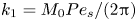$k_1 = M_0Pe_s/(2{\rm \pi} )$, leads to

(4.23) \begin{equation} {k_2 = \mathrm{i} \dfrac{\sqrt{2}}{2}\dfrac{\Gamma\left(\dfrac{M_0Pe_s}{4{\rm \pi}}\right)}{\Gamma\left(\dfrac{1}{2}+\dfrac{M_0Pe_s}{4{\rm \pi}}\right)}}, \end{equation}

where $\Gamma \left (\,\,\right )$ is the gamma function and should not be confused with the surfactant concentration $\varGamma$, which is italicized throughout the paper. Undoing the change of variables (4.16), the final form of the similarity solution is

(4.24a) \begin{equation} {f(\eta) =\frac{- 6\,\Gamma\left(\dfrac{1}{2}+\zeta\right){}_1F_1\left(\dfrac{1}{2}+\zeta\,;\dfrac{3}{2}\,;-\dfrac{\eta^2}{2}\right) + 6\sqrt{2}\,\mathrm{i}\,\eta\,\Gamma\left(1+\zeta\right){}_1F_1\left(1+\zeta\,;\dfrac{3}{2}\,;-\dfrac{\eta^2}{2}\right) +\, 4\,\eta^2\,\Gamma\left(\dfrac{3}{2}+\zeta\right){}_1F_1\left(\dfrac{3}{2}+\zeta\,;\dfrac{5}{2}\,;-\dfrac{\eta^2}{2}\right)} {3\sqrt{2}\,\mathrm{i}\,\Gamma\left(\zeta\right){}_1F_1\left(\zeta\,;\dfrac{1}{2}\,;-\dfrac{\eta^2}{2}\right) + 6\eta\,\Gamma\left(\dfrac{1}{2}+\zeta\right){}_1F_1\left(\dfrac{1}{2}+\zeta\,;\dfrac{3}{2}\,;-\dfrac{\eta^2}{2}\right) }}, \end{equation}

where we have defined

(4.24b)\begin{equation} \zeta := \dfrac{M_0Pe_s}{4{\rm \pi}}. \end{equation}

The solution given by (4.24) is equivalent to the fundamental solution derived by Bickel & Detcheverry (Reference Bickel and Detcheverry2022) using the Cole–Hopf transformation with a Dirac distribution as the initial condition. Figure 4 displays an initially rectangular pulse of surfactant spreading following Burgers equation (2.18a), for different values of the surface Péclet number. When advection is negligible and $Pe_s\ll {1}$, the solution quickly becomes Gaussian in shape, converging towards the fundamental solution of the (linear) diffusion equation. This occurs on times of order $t= O(Pe_s)$, since at small $Pe_s$ the dominant balance in (2.18a) modifies the characteristic time scale, which we had assumed to be set by advection in § 2. As $Pe_s$ increases and reaches an advection-dominated regime $Pe_s\gg {1}$, the solution changes shape, resembling the semicircular surfactant profile of the purely advective solution (4.6) of the previous subsection.

Figure 4. Spreading solutions for an initially rectangular pulse of surfactant, with a functional form given in Appendix E, for (a) $Pe_s=1/50$, (b) $Pe_s=1$ and (c) $Pe_s=50$. For each example, panels (a i,iii,b i,iii,c i,iii) show the concentration $\varGamma (x,t)$ and interfacial velocity $u_s(x,t)$ obtained through the exact solution of (2.18), while panels (a ii,iv,b ii,iv,c ii,iv) show the same data rescaled in similarity variables (colour curves), superimposed on the similarity solution (4.24) (black curves) valid at long times $t\gg {1}$. In all examples, $x_*=t_*=0$.

5.1. Dimple solutions

The first dimple distribution we consider is $\varGamma _0(x)=x^2/(1+x^2)$ (which we call the ‘Cauchy dimple’) since it has already been studied by Crowdy (Reference Crowdy2021b) and Bickel & Detcheverry (Reference Bickel and Detcheverry2022). It has a quadratic minimum $\varGamma _0(x)\sim {x}^2$ around $x=0$ and, since it is a symmetric distribution, it follows from the method of characteristics (see Appendix D) that $u_*=x_*=0$ and $t_*=1$. The exact evolution of a Cauchy dimple is displayed in figure 5(a i,iv), with the surfactant concentration reaching a cusp-like singularity at $t_*$ and $x_*$. Figures 5(b i,iv) and 5(c i,iv) displays the evolution of other profiles $\varGamma _0(x)$ with different functional forms (detailed in Appendix E), but always with a quadratic minimum to ensure that they display the same similarity behaviour. Self-similarity appears locally, for positions and times close enough to $x_*$ and $t_*$, respectively. As discussed in § 3.2, the self-similar solution that appears prior to $t_*$ is dubbed the ‘closure’ solution, since here the concentration remains zero $\varGamma (x_*,t)=0$ at all times. After the dimple ‘closes’ at $t_*$, a different ‘levelling’ solution appears, whereby the concentration starts levelling towards the final steady distribution $\varGamma (x,t)={1}$.

Figure 5. Filling solutions with $Pe_s^{-1}=0$, for initial ‘dimple’ distributions of surfactant given by (a) a Cauchy dimple, (b) a squared Cauchy dimple and (c) an arctangent dimple, with their functional forms given in Appendix E. For each example, panels (a i,iv,b i,iv,c i,iv) show the concentration $\varGamma (x,t)$ and interfacial velocity $u_s(x,t)$ obtained through the exact solution of (2.19). Panels (a ii,v,b ii,v,c ii,v) and (a iii,vi,b iii,vi,c iii,vi) show exact solutions rescaled in similarity variables (colour curves), superimposed on the closure (5.7) and levelling (5.5) similarity solutions (black curves) valid prior and subsequent to the singularity, respectively. In all examples, $x_*=0$.

It is shown in § 3.2 that the similarity exponent for dimple solutions is $\beta =2$, which can be substituted in the implicit similarity solution (3.2) to yield

(5.2)\begin{equation} \mathrm{sgn}\left(\eta\right)k_\pm{f}^2+f-\eta = 0. \end{equation}

Solutions to (5.2) represent both (pre-singularity) closure solutions and (post-singularity) levelling solutions, which have expansions around $\eta =0$ (table 2) given by $f(\eta )\sim \eta +\mathrm {i}{K}\eta ^2$ and $f(\eta )\sim \mathrm {i}{K}-\eta$, respectively. Both of these expansions lead to imaginary constants $k_\pm$ when introduced in (5.2). This means that, due to the symmetry condition $k_-=\bar {k}_+$ (3.3), we can consider a single constant $k=k_+=-k_-=\mathrm {sgn}\left (\eta \right )k_\pm$. Solving (5.2),

(5.3)\begin{equation} f(\eta) = \dfrac{-1\pm\sqrt{1+4k\eta}}{2k}. \end{equation}

For the levelling solution, we expect $\psi (x_*,t)$, and thus $f(0)$, to be non-zero, which leads us to choose the minus sign in (5.3). This sign choice must be valid for all $\eta$ since a change from $-$ to $+$ requires the square root to be zero to maintain a continuous solution, while the radicand $1+4k\eta$ can never be zero with $k$ imaginary. We also fix ${k=\mathrm {i}}$ so that ${f(0)=\mathrm {i}}$ (or, equivalently, $C(0)=1$). The dimple levelling solution is then

(5.4)\begin{equation} {f(\eta)=\dfrac{\mathrm{i}}{2}\left(\sqrt{1+4\mathrm{i}\eta}+1\right)}, \end{equation}

which can alternatively be decomposed into its real and imaginary parts using the relation $\sqrt {z}=\sqrt {(|z|+\mathrm {Re}\left [z\right ])/2}+\mathrm {i}\,\mathrm {sgn}\left (\mathrm {Im}\left [z\right ]\right )\sqrt {(|z|-\mathrm {Re}\left [z\right ])/2}$, leading to

(5.5a)$$\begin{gather} C(\eta) = \dfrac{1}{2}\left(\sqrt{\dfrac{1}{2}\left[\sqrt{1+16\eta^2}+1\right]}+1\right), \end{gather}$$

(5.5b)$$\begin{gather}U(\eta) ={-}\dfrac{1}{2}\,\mathrm{sgn}\left(\eta\right)\sqrt{\dfrac{1}{2}\left[\sqrt{1+16\eta^2}-1\right]}. \end{gather}$$

We note that (5.5) leads to $C(\eta )\sim (\sqrt {2}/2){\,|\eta |^{1/2}}$ and $U(\eta )\sim -\mathrm {sgn}\left (\eta \right )(\sqrt {2}/2){\,|\eta |^{1/2}}$ as $|\eta |\to \infty$, compatible with the far field condition (2.26).

For the closure solution, the choice in (5.3) must be the plus sign such that $f(0)=0$. In the absence of an obvious choice for an integration constant $k$ (since $U(0)=C(0)=0$), we fix its value so that the far-field behaviour of the closure solution is equivalent to that of the levelling solution (5.5). In other words, we require $C(\eta )\sim (\sqrt {2}/2){\,|\eta |^{1/2}}$ and $U(\eta )\sim \mathrm {sgn}\left (\eta \right )(\sqrt {2}/2){\,|\eta |^{1/2}}$ as $|\eta |\to \infty$, where the sign change in $U(\eta )$ is due to the reversal in the sign of $x$ between the definitions of the similarity variable (2.22a) and (2.22b) for each solution. This leads to $f(\eta )\sim {e}^{{\mathrm {i}{\rm \pi} }/{4}}\eta ^{1/2}$ as $\eta \to \infty$, which introduced in (5.2) results in $k=-\mathrm {i}$. The final form of the dimple closure solution is then

(5.6)\begin{equation} {f(\eta)=\dfrac{\mathrm{i}}{2}\left(\sqrt{1-4\mathrm{i}\eta}-1\right)}, \end{equation}

from which we obtain

(5.7a)$$\begin{gather} C(\eta) = \dfrac{1}{2}\left(\sqrt{\dfrac{1}{2}\left[\sqrt{1+16\eta^2}+1\right]}-1\right), \end{gather}$$

(5.7b)$$\begin{gather}U(\eta) = \dfrac{1}{2}\,\mathrm{sgn}\left(\eta\right)\sqrt{\dfrac{1}{2}\left[\sqrt{1+16\eta^2}-1\right]}. \end{gather}$$

The choice of (5.4) and (5.6) having an equivalent far-field behaviour ensures that the multiplicative constant $A$ in the similarity formulation (2.20) is the same for both the closure and the levelling solutions. This fact simplifies calculations, since it then suffices to compute $A$ for only one of the two solutions.

Figure 5(a ii,v,b ii,v,c ii,v) shows how the exact solutions converge to the closure self-similar profiles given by (5.6) before the singularity, for the three distinct initial profiles $\varGamma _0(x)$ considered. Likewise, figure 5(a iii,vi,b iii,vi,c iii,vi) illustrates that exact solutions converge to the levelling solution (5.4) after the singularity. Since the similarity solutions are only valid locally, the agreement between the rescaled profiles is always improved as $t\to {t_*}$ or as $x\to {x_*}$.

5.2. Hole solutions

Contrary to dimples, hole similarity solutions (with $\beta =3/2$) had not yet been identified for the complex inviscid Burgers equation (2.19a). One of the simplest examples of a distribution of surfactant that satisfies this condition is a ‘rectangular hole’ with $\varGamma _0(x)=H(|x|-1)$, where $H(x)$ is the Heaviside step function, which we illustrate in figure 6(a). For this case, the initial surfactant profile is even and therefore its Hilbert transform $u_{s0}(x)=\mathcal {H}\left [\varGamma _0(x)\right ]$ is odd, which implies (see Appendix D) that the position of the singularity is $x_*=0$, its velocity $u_*=0$, and the closure time $t_*={\rm \pi} /2$. One can also easily verify that $\varGamma _0''(0)=u_{s0}''(0)=0$ and thus the condition for hole self-similar solutions $\psi _0''(x_*-u_*t_*)=\psi _0''(0)=0$ is satisfied. Figure 6(a) depicts the exact evolution of the rectangular hole according to the inviscid Burgers equation (2.19a). As for the case of dimples, the distribution first goes through a ‘closure’ phase where surfactant is advected inwards but remains $\varGamma (0,t)=0$ at the origin. However, figure 6(a) also shows that the self-similar dynamics before the closure time $t_*$ must be different from that of the dimple, since the solution retains a finite interval around $x_*=0$ where the concentration remains zero. After $t_*={\rm \pi} /2$, the concentration at the origin starts ‘levelling’, with $\varGamma (0,t)>0$, until the profile reaches a homogeneous distribution $\varGamma (x,t)=1$ as $t\to \infty$.

Figure 6. Filling solutions with $Pe_s^{-1}=0$, for initial ‘hole’ distributions of surfactant given by (a) a rectangular hole, (b) a quartic hole and (c) an asymmetric hole, with their functional forms given in Appendix E. For each example, panels (a i,iv,b i,iv,c i,iv) show the concentration $\varGamma (x,t)$ and interfacial velocity $u_s(x,t)$ obtained through the exact solution of (2.19). Panels (a ii,v,b ii,v,c ii,v) and (a iii,vi,b iii,vi,c iii,vi) show exact solutions rescaled in similarity variables (colour curves), superimposed on the closure (5.13) and levelling (5.10) similarity solutions (black curves) valid prior and subsequent to the singularity, respectively. The asymmetric hole (c) has $x_*\approx {0.562}$, otherwise $x_*=0$.

In this case, the self-similar solutions can also be obtained in closed form by substituting $\beta =3/2$ in the implicit solution given by (3.2), which leads to

(5.8)\begin{equation} k_\pm f^3 + f - \eta = 0. \end{equation}

Substituting the expansions around $\eta =0$ found in table 2 for the closure ($\,f\sim \eta +K\eta ^3$) and levelling solutions ($f\sim -\mathrm {i}{K}-\eta /2$) into (5.8) leads to real constants $k_\pm$. Combined with the symmetry condition (3.3), this indicates that for either solution we can consider a single constant $k=k_-=k_+$, as in the case of spreading pulse solutions of § 4.1.

We first solve (5.8) for the case of the (post-singularity) levelling solution. We again choose to fix ${f(0)=\mathrm {i}}$ or, equivalently, $C(0)=1$, which results in $k=1$. The discriminant of the cubic (5.8) is then $-4-27\eta ^2$, which is negative for any $\eta$. This implies that (5.8), for any given value of $\eta$, has one real and two complex conjugate solutions that can be obtained using standard methods for solving cubic equations (Cox Reference Cox2012). Choosing the complex solution with a positive imaginary part results in the hole levelling solution

(5.9) \begin{equation} {f(\eta) = {\rm e}^{{\mathrm{i}{\rm \pi}}/{3}}\sqrt[{3}]{\dfrac{1}{2}\left[\sqrt{\eta^2+\dfrac{4}{27}}-\eta\right]} + {\rm e}^{{2\mathrm{i}{\rm \pi}}/{3}}\sqrt[{3}]{\dfrac{1}{2}\left[\sqrt{\eta^2+\dfrac{4}{27}}+\eta\right]}}. \end{equation}

Furthermore, since the arguments of the two cubic roots in (5.9) are always real and positive, it is straightforward to decompose the expression into

(5.10a)$$\begin{gather} C(\eta) = \dfrac{\sqrt{3}}{2}\left(\sqrt[{3}]{\dfrac{1}{2}\left[ \sqrt{\eta^2+\dfrac{4}{27}}-\eta\right]}+\sqrt[{3}]{\dfrac{1}{2}\left[\sqrt{\eta^2+\dfrac{4}{27}}+\eta\right]}\right), \end{gather}$$

(5.10b)$$\begin{gather}U(\eta) = \dfrac{1}{2}\left(\sqrt[{3}]{\dfrac{1}{2}\left[ \sqrt{\eta^2+\dfrac{4}{27}}-\eta\right]}-\sqrt[{3}]{\dfrac{1}{2}\left[\sqrt{\eta^2+\dfrac{4}{27}}+\eta\right]}\right), \end{gather}$$

where the far-field behaviour $|\eta |\to \infty$ is in this case given by $C(\eta )\sim (\sqrt {3}/2){|\eta |^{1/3}}$ and $U(\eta )\sim -\,\mathrm {sgn}\left (\eta \right )(1/2){\,|\eta |^{1/3}}$.

In the case of the closure solution, we again choose the integration constant such that its far field is equivalent to that of the levelling solution, which requires $k=-1$. As in the case of dimples, this choice of far field ensures that the scaling constant $A$ in the similarity formulation (2.20) is the same for both closure and levelling. The discriminant of (5.8) is then $4-27\eta ^2$, which indicates that its three solutions are real for $|\eta |\leq \sqrt {4/27}=2\sqrt {3}/9$, whereas for $|\eta |\geq 2\sqrt {3}/9$ there is one real and two complex conjugate solutions. The only way to ensure a continuous solution with $C(\eta )>0$ is to define $f(\eta )$ piecewise, with one of the three solutions of the cubic valid for ${\eta \leq -2\sqrt {3}/9}$, and another one valid for ${\eta \geq -2\sqrt {3}/9}$. Such a solution is

(5.11)\begin{align} {f(\eta)=} \begin{cases} {{\rm e}^{{\mathrm{i}{\rm \pi}}/{3}}\left(\sqrt[{3}]{-\dfrac{1}{2}\left[\sqrt{\eta^2-\dfrac{4}{27}}-\eta\right]}-\sqrt[{3}]{-\dfrac{1}{2}\left[\sqrt{\eta^2-\dfrac{4}{27}}+\eta\right]}\right)} , & {\text{if }\eta\leq{-}\dfrac{2\sqrt{3}}{9}},\\ {{\rm e}^{{\mathrm{i}{\rm \pi}}/{3}}\left(\sqrt[{3}]{\phantom{-}\dfrac{1}{2}\left[\sqrt{\eta^2-\dfrac{4}{27}}+\eta\right]}-\sqrt[{3}]{\phantom{-}\dfrac{1}{2}\left[\sqrt{\eta^2-\dfrac{4}{27}}-\eta\right]}\right)} , & {\text{if }\eta\geq{-}\dfrac{2\sqrt{3}}{9}}, \end{cases} \end{align}

which can be expressed more compactly as

(5.12) \begin{align} {f(\eta) = {\rm e}^{{\mathrm{i}{\rm \pi}}/{3}} \left( \sqrt[{3}]{\frac{1}{2}\left[\sqrt{\eta+\frac{2\sqrt{3}}{9}}\sqrt{\eta-\frac{2\sqrt{3}}{9}}+\eta\right]} - \sqrt[{3}]{\dfrac{1}{2}\left[\sqrt{\eta+\dfrac{2\sqrt{3}}{9}}\sqrt{\eta-\dfrac{2\sqrt{3}}{9}}-\eta\right]} \,\right)}. \end{align}

For $|\eta |\geq 2\sqrt {3}/9$, the argument of the cubic roots in (5.12) is always real, leading to a straightforward decomposition into real and imaginary parts. However, in the case of $|\eta |\leq 2\sqrt {3}/9$, the real and imaginary parts of the solution can only be obtained through the trigonometric solution of the cubic (Cox Reference Cox2012). In summary, the final form of the similarity solutions $C(\eta )$ and $U(\eta )$ is

(5.13a) $$\begin{gather} C(\eta) = \begin{cases} 0 & \text{for }|\eta|\leq\dfrac{2\sqrt{3}}{9},\\ \dfrac{\sqrt{3}}{2}\left(\sqrt[{3}]{\dfrac{1}{2}\left[|\eta|+\sqrt{\eta^2-\dfrac{4}{27}}\right]}-\sqrt[{3}]{\dfrac{1}{2}\left[|\eta|-\sqrt{\eta^2-\dfrac{4}{27}}\right]}\right) & \text{for }|\eta|\geq\dfrac{2\sqrt{3}}{9}, \end{cases} \end{gather}$$

(5.13b) $$\begin{gather}U(\eta) = \begin{cases} \dfrac{2\sqrt{3}}{3}\sin\left[\dfrac{1}{3}\arcsin\left(\dfrac{3\sqrt{3}}{2}\eta\right)\right], & \text{for }|\eta|\leq\dfrac{2\sqrt{3}}{9},\\ \dfrac{1}{2}\mathrm{sgn}\left(\eta\right)\left(\sqrt[{3}]{\dfrac{1}{2}\left[|\eta|+\sqrt{\eta^2-\dfrac{4}{27}}\right]}\hspace{-1.5pt}+ \sqrt[{3}]{\dfrac{1}{2}\left[|\eta|-\sqrt{\eta^2-\dfrac{4}{27}}\right]}\right), & \text{for }|\eta|\geq\dfrac{2\sqrt{3}}{9}, \end{cases} \end{gather}$$

where we can verify that its far field as $|\eta |\to \infty$, which is given by $C(\eta )\sim (\sqrt {3}/2){|\eta |^{1/3}}$ and $U(\eta )\sim \mathrm {sgn}\left (\eta \right )(1/2){|\eta |^{1/3}}$, is equivalent to that of the levelling solution.

Figures 6(a ii,v) and 6(a iii,vi) show that the exact solution, when appropriately rescaled using (2.20), converges to the closure solution (5.13) before $t_*$ and to the levelling solution (5.10) after $t_*$. Other initial surfactant profiles also lead to these similarity solutions, as long as the condition $\psi _0''(x_*-t_*u_*)=0$ is met. It is worth noting that the initial surfactant distribution does not need to be zero at a finite interval to tend to a self-similar solution for a hole, as exemplified by the ‘quartic hole’ initial condition $\varGamma _0(x)=x^4/(1+x^4)$, whose evolution is displayed in figure 6(b). This initial profile also has even symmetry, leading to $x_*=0$, $u_*=0$, and $t_*=\sqrt {2}$ (see Appendix D), but its initial concentration is zero only at the origin $x_*=0$. Regardless, since $\psi _0''(x_*-u_*t_*)=\psi _0''(0)=0$, the profiles evolve towards the closure solution (5.12) for $t< t_*$ (figure 6b ii,v) and towards the levelling solution (5.9) for $t>t_*$ (figure 6b iii,vi). Even though $\varGamma _0(x)$ is zero at a single point, the concentration ‘flattens’ as $t\to {t_*}$ to converge towards a solution that is zero at a finite interval.

The last example illustrated in figure 6(c) is an asymmetric initial condition. For this case, we have that $x_*\neq {0}$ and $u_*\neq {0}$, although their values can still be calculated from the method of characteristics, as detailed in Appendix D. The self-similar dynamics is still governed by the solutions (5.12) and (5.9) although, since the point of the singularity moves with $u_*\neq {0}$, the similarity variable must account for a frame of reference moving with the singular point. This leads to a more general similarity ansatz

(5.14a)$$\begin{gather} \psi(x,t) = u_* + A|t-t_*|^{\beta-1}f(\eta), \end{gather}$$

(5.14b)$$\begin{gather}\eta = \mathrm{sgn}\left(t-t_*\right) \dfrac{x-\left[x_*+u_*(t-t_*)\right]}{A|t-t_*|^\beta}. \end{gather}$$

Equation (5.14) accounts for the moving singular point, whose position is $x_s(t)=x_*+u_*(t-t_*)$. Note that $x_s(t_*)=x_*$, whereas $x_s(0)=x_*-u_*t_*$, which is the departure position of the moving singular point.