5.1. Thermal waves’ pumping effect

When there is no flow in the channel, a thermal wave acting on the lower wall can pump fluid horizontally at a rate $Q$ in the direction opposite to wave propagation. The flow response for a wave travelling to the right is a mirror image of the response for a wave travelling to the left; $Q$ is positive for the leftward wave, whereas it is negative for the rightward wave. Figure 2(a) shows that an increase in wave velocity $|c|$ increases $|Q|$ at the rate proportional to ${\sim }|c|$, but after reaching a maximum, its further increase reduces $|Q|$ proportionally to ${\sim }|c|^{-4}$. Figure 2(b) demonstrates that an excessive increase in the wave wavelength reduces $|Q|$ proportionally to $\sim \alpha ^4$, whereas an excessive reduction reduces $|Q|$ proportionally to $\sim \alpha ^{-6}$. The largest $|Q|$ occurs for waves with the wavenumbers $\alpha \in [1,4]$ and phase speed $|c| \in [1,5]$. An increase in the wave amplitude $Ra_{p,L}$ increases the flow rate proportionally to $\sim Ra_{p,L} ^2$, as shown in figure 2(c), but an excessively large amplitude slows down the increase due to various saturation effects. The pumping effect is known to be associated with the propulsion provided by the convection rollers (see figure 3) formed due to wave diffusion into the channel interior. At large $|c|$ and $\alpha$, these rollers appear very near to the lower wall, forming a boundary layer and reducing $|Q|$ drastically.

Figure 2. (a) Variation of the flow rate correction $Q_c$ as a function of the wave speed $c$, (b) wave wavenumber $\alpha$ and (c) wave amplitude $Ra_{p.L}$ for $Re =0$, $Pr=0.71$. Asymptotes are depicted by dashed lines. In (a,c) $\alpha =2$, and in (b) $Ra_{p.L}=1000$.

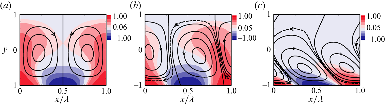
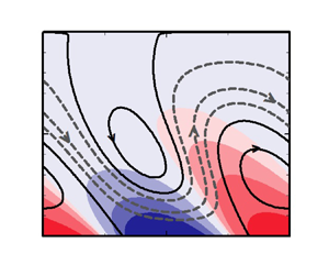
Figure 3. Flow topology (line) and temperature (filled colour) field at $Re =0$ with (a) $c=0$, (b) $c=2$ and (c) $c=20$ for $Ra_{p,L}=1000$, $\alpha =2$, $Pr=0.71$. The dashed lines show the meandering flow stream. Arrows show the stream flow direction.

Variations of flow topology associated with variation of $c$ are illustrated in figure 3. As the waves diffuse into the channel interior, they are delayed by the fluid thermal inertia, with their positions falling farther behind the surface waves as the distance from the lower wall increases. This process results in bubbles tilting. We refer to this effect as the lagging thermal penetration. The bubble tilting occurs leftward when the wave travels rightward ($c> 0$), and rightward when the wave travels leftward ($c < 0$).

5.2. Flow modifications generated by thermal waves

There is an established isothermal flow from left to right characterized by $Re$. This flow is modified by a thermal wave with wave velocity $c$ applied at the lower wall. Its response depends on $Re$ and $c$. A stationary wave ($c=0$) represents the reference configuration with flow topology displayed in figure 4. The topology for $Re=0$ consists of pairs of counter-rotating rolls and has vertical mushroom-shaped isotherms (figure 4a). Introduction of a weak flow, e.g. $Re=1$, causes these rolls to separate, creating a narrow meandering stream between them (figure 4b). The rolls morph into upper and lower wall separation bubbles, with the upper bubbles rotating anticlockwise and the lower bubbles rotating clockwise. The bubbles and isotherms are slightly tilted rightward. Further, an increase in $Re$ eliminates the upper bubbles (figure 4c), reduces the size of the lower bubbles and increases the rightward tilt of the bubbles and isotherms. A fast enough flow (e.g. $Re>20$) washes away even the lower bubbles, bringing the flow to a parallel form (figure 4d), with the titled isotherms concentrated only near the lower wall. The flow advects a portion of the applied wall heat horizontally, and the rest diffuses into the interior of the channel. We refer to this as leading thermal penetration, resulting in the bubbles and isotherms tilting along the flow direction.

Figure 4. Flow topology (line) and temperature (filled colour) field at $c=0$ with (a) $Re=0$, (b) $Re=1$, (c) $Re=10$, (d) $Re=20$ for $Ra_{p,L}=1000$, $\alpha =2$, $Pr=0.71$. The grey dashed lines show the meandering flow stream. Arrows show the stream flow direction.

Response to the moving wave is illustrated in figure 5 for $Re=1$ flow. The flow topology remains qualitatively similar for larger $Re$ (not shown), with the bubbles decreasing in size. The use of low-velocity waves ($c=1$) directed along the flow direction results in an appearance of a rightward (i.e. towards flow direction) shift of the position of the bubbles (figure 5a), which is mainly due to the formation of a thicker stream tube carrying fluid to the right. The upper bubbles shift to the left and exhibit right tilting (figure 5b). Further increase of $c$ eventually eliminates the bubbles (figure 5c,d). The tilting is caused by delay associated with heat diffusion into the flow interior (the rightward wave movement is faster than the heat diffusion across the stream), i.e. thermal lagging. Reversing the wave's direction to opposite the flow (see figure 5e–h) has qualitatively similar effects on the bubbles’ sizes and their eventual elimination but causes rightward tilt, which increases with the wave velocity. One can note that thermal lagging causes tilting along flow direction when the wave travels leftward ($c<0$). The rightward wave ($c>0$) produces tilting in the direction opposite to the flow.

Figure 5. Flow topology (line) and temperature (filled colour) field at $Re=1$ with (a) $c=1$, (b) $c=10$, (c) $c=20$, (d) $c=70$, (e) $c=-1$, ( f) $c=-10$, (g) $c=-20$ and (h) $c=-70$ for $Ra_{p,L}=1000$, $\alpha =2$, $Pr=0.71$. The grey dashed lines show the meandering flow stream. Arrows show the stream flow direction.

The effects of $Re$ and $c$ can be gleaned from figure 6, displaying variations of the correction factor $\varGamma _{cor}=Q_c/(\frac {4}{3}Re)$ defined in (2.8), as a function of $Re$ and $c$. Conditions leading to the reduction of flow losses are marked using grey colour. A characteristic, nearly straight line separates the resistance-reducing from the resistance-increasing waves. Conditions along this line identify the critical wave speed $c_n$ and the critical Reynolds number $Re_n$, with $c_n = 0.77 Re_n$, which results in zero flow rate correction $Q_c=0$. The countercurrent waves always reduce flow resistance. Their effectiveness is largest for small $Re$ where they can increase flow rate up to ${\sim }20$ times compared with the reference isothermal flow. The cocurrent waves also reduce resistance, but such waves cannot be too fast as fast enough waves increase resistance. Such waves are less effective than countercurrent waves, providing only up to 20 % flow rate increase. These results demonstrate a potential for significantly reducing flow losses by waves with proper characteristics.

Figure 6. Variation of the correction factor $\varGamma _{cor}$ as a function of Reynolds number $Re$ and wave speed $c$ for $\alpha =2$, $Ra_{p,L} =1000$, $Pr=0.71$. Grey shaded zone identifies conditions leading to flow rate increase with respect to the reference isothermal flow. The thick line illustrates variation of the critical Reynolds number $Re_n$ as a function of the critical wave velocity $c_n$, which can be approximated as $c_n = 0.77 Re_n$. Vertical (purple) and horizontal (blue) dotted lines identify conditions used in figures 9 and 10, respectively.

We shall now discuss how waves affect flow structures. The introduction of waves activate three effects. The first one is the reduction of direct contact between the stream and the bounding walls, which reduces friction experienced by the stream. The second one involves additional propulsion generated by the bubbles’ rotation as the bubbles rotate in the stream direction, which is favourable to the flow. The third one is flow blockage by the bubbles (reduction of flow cross-sectional area), which increases flow losses. As $Re$ increases, bubbles are eventually washed away, eliminating the resistance-reducing effect. The net effect of waves on the flow rate can be determined by integrating the modal function $u^{(0)}$ across the channel. Figure 7 illustrates the distribution of this function for a variety of conditions. A wave with critical velocity $c_n=0.77$ produces modal function $u^{(0)}=0$ across the channel, thus no change in the flow rate. Other waves generally produce large flow rate changes in the upper portion of the channel and relatively smaller changes in the lower portion, so the upper portion determines the overall flow rate correction. Waves with $c< c_n$ (countercurrent waves and sufficiently slow cocurrent waves) produce a large flow rate increase in the upper portion of the channel and the overall flow rate increase, while sufficiently fast cocurrent waves produce large flow rate decrease in the upper portion and the overall flow rate decrease.

Figure 7. Distribution of the modal function $u^{(0)}$ for selected values of $c$ at $Re = 1$, $Ra_{p,L} = 1000$, $\alpha = 2$, $Pr = 0.71$.

Wave action changes wall shear, which may increase or decrease depending on the flow conditions and wave characteristics. Change in the shear is responsible for the change in the flow rate. Distributions of shear modifications for different wave velocities, propagation directions and flow Reynolds numbers are displayed in figures 8(a) and 8(b). The shear distribution is symmetric for waves with velocity $c_n$, producing a zero mean value. Waves with $c \ne c_n$ break this symmetry, producing a net shear force with the modifications equal and opposite in the lower and upper walls. Waves travelling opposite to the flow ($c<0$) and sufficiently slow waves travelling in the flow direction ($c< c_n$) produce positive modification at the lower wall, whereas sufficiently fast waves travelling in the flow direction ($c>c_n$) produce negative modifications. When mean shear at $c=c_n$ is used as a reference point, an increase of $|c-c_n|$ causes the magnitude of the average shear modification to initially increases, attains a maximum and then decrease with a further increase of $|c-c_n|$ (figure 8c). The decrease at large $|c|$ is proportionally to $|c|^{-4}$ (see Appendix B for discussion on the asymptote).

Figure 8. Wall shear force modification $\tau _{mod}$ profiles and mean shear modifications $\tau _{av}$ at the (a) lower and (b) upper wall for selected values of $c$ at $Re = 1$, $Ra_{p,L} = 1000$, $\alpha = 2$, $Pr = 0.71$. Subscripts $L$ and $U$ denote the lower and upper wall, respectively. The dotted line shows shear for $c_n=0.77$. Panel (c) displays the average wall shear force modification at the lower wall and in this figure, solid and dashed lines show positive and negative values, respectively. Large $c$ asymptotes are shown by dotted lines.

Variations of the flow rate correction $Q_c$ as a function of $c$ are illustrated in detail in figure 9 for $Re=1$, 10, 20. The critical wave velocity for each $Re$ is $c_n=0.77$, 7.7, 15.4, respectively; $c< c_n$ provides positive flow rate correction, causing an overall decrease of flow resistance, but $c>c_n$ provides negative flow rate correction, causing the overall increase in flow resistance. When $c$ either increases or decreases away from $c_n$, the flow rate correction exhibits a qualitatively similar response – its magnitude initially increases, attains a maximum and then gradually decreases, eventually becoming proportionally to $|c|^{-4}$.

Figure 9. Variation of the flow rate correction $Q_c$ as a function of wave speed $c$ for selected values of $Re$. Solid and dashed lines show positive and negative values, respectively. Large $c$ asymptotes are shown by dotted lines. Flow conditions used in this figure are identified by purple dotted lines in figure 6.

Figure 10 illustrates in more detail how an increase of $Re$ affects $Q_c$. The selected curves corresponding to $c=0, \pm 0.1, \pm 2$ and $\pm 10$ illustrate how the flow response changes with the wave direction change and clearly identify the change from an increase of the flow rate to its decrease as $Re$ increases. There are well-defined limits of $Q_c$ for $Re\rightarrow 0$, which are positive for negative $c$ and negative for positive $c$, with $c=0$ representing the boundary between them characterized by $Q_c \rightarrow 0$ with $Re \rightarrow 0$. The case of $Re=0$ corresponds to the pumping problem studied in Hossain & Floryan (Reference Hossain and Floryan2023) and briefly reviewed in § 5.1. It is interesting to note that in the case of $c=0$, $Q_c$ initially increases proportionally to $Re$, attains a maximum and then decreases with the further increase of $Re$ proportionally to $Re ^ {-2.5}$. Countercurrent waves produce $Q_c$ changing marginally with $Re$ until $Re$ becomes large enough to cause a decrease proportional to $Re ^ { -2.5}$. The behaviour of cocurrent waves is qualitatively similar if one considers $|Q_c|$, i.e. there is a well-defined limit for small $Re$ and well-defined behaviour for large $Re$, except in the neighbourhood of $Re=Re_n$ where $Q_c$ passes through zero. A countercurrent wave, a wave travelling opposite the flow ($c < 0$), always provides $Q_c > 0$. The cocurrent wave, a wave travelling along the flow ($c > 0$), increases flow losses if $Re< Re_n$ and decreases flow losses when $Re>Re_n$. One, of course, needs to remember that a flow that is too fast ($Re$ too big) washes away bubbles, and the flow resistance loses any dependence on the thermal waves.

Figure 10. Variation of the flow rate correction $Q_c$ as a function of Reynolds number $Re$ for selected values of $c$. Solid and dashed lines show positive and negative values, respectively. Small and large $Re$ asymptotes are shown by dotted lines. Flow conditions used in this figure are identified by blue dotted lines in figure 6.

Effects of a wave's wavelength are illustrated in figure 11. As the wavenumber increases, the countercurrent waves reduce resistance ($Q_c >0$) proportionally to ${\sim }\alpha ^4$, the resistance reduction attains a maximum and then decreases proportionally to ${\sim }\alpha ^{-6}$ (details of the analysis are given in § 6). Cocurrent waves exhibit a similar trend but with a notable difference. They reduce resistance ($Q_c>0$) if they are sufficiently slow and increase resistance if they are fast enough. An estimate of the critical velocity $c_n$ can be obtained from analytical solutions for large and small $\alpha$, i.e.

(5.1a)$$\begin{gather} c_{n} = \frac{(1929+3130 Pr)Re}{3435(1+Pr)} \quad \alpha \rightarrow 0, \end{gather}$$

(5.1b)$$\begin{gather}c_{n} = \frac{(27+22Pr)Re}{4 \alpha(1+Pr)} \quad \alpha \rightarrow \infty. \end{gather}$$

Figure 11. Variation of the flow rate correction $Q_c$ as a function of wave wavenumber $\alpha$ for selected values of $c$ at $Ra_{p,L}$ =1000, $Re=1$, $Pr=0.71$. Solid and dashed lines show positive and negative, respectively. Large and small $\alpha$ asymptotes are shown by dotted lines.

Variations of $\varGamma _{cor}$ as a function of $c$ and $\alpha$ displayed in figure 12 permit a quick identification of the most effective waves. Waves with $\alpha \approx 2$ and $c \in [-2, -3]$ produce the largest resistance reduction, and waves with $\alpha \approx 2$ and $c \in [3, 5]$ produce the largest resistance increase. The maximum resistance reduction occurs for $\alpha = \alpha _{max} \approx 2$ with $\alpha _{max}$ decreases marginally with $c$. The reader may note that the critical wave velocity $c_n$ varies marginally as a function of $\alpha$.

Figure 12. Variation of the correction factor $\varGamma _{cor}$ as functions of wave wavenumber $\alpha$ and wave speed $c$ for $Re=1$, $Ra_{p,L}=1000$, $Pr=0.71$. Grey shaded zone identifies conditions leading to an increase of the flow rate above the flow rate in the reference isothermal channel.

Results displayed in figure 13 demonstrate that the magnitude of change of resistance initially increases proportionally to ${\sim }Ra_{p,L}^2$ . This growth slows down for $Ra_{p,L}> \sim 2000$ due to saturation effects, which suggests that excessively large heating is not beneficial. Also, the results of stability analysis discussed in § 7 suggest a possible transition to secondary states for excessively large wave amplitudes.

Figure 13. Variation of the flow rate correction $Q_c$ as a function of wave intensity $Ra_{p,L}$ for selected values of $c$ at $\alpha =2$, $Re=1$, $Pr=0.71$. Solid and dashed lines show positive and negative values, respectively. Small $Ra_{p,L}$ asymptote is shown by dotted lines.

One may wish to ascertain the effectiveness of a moving thermal wave over a stationary heating pattern. Figure 14 displays variations of the stationary gain factor $\varGamma _s$, defined as

(5.2)\begin{equation} \varGamma_s = \frac{Q_c-Q_c|_{c=0}}{Q_c|_{c=0}}, \end{equation}

with $Q_c|_{c=0}$ denoting the flow rate correction when $c=0$. Positive values of $\varGamma _s$ correspond to the moving wave being more effective. Variation of the critical wave velocity $c_n=0.77Re$ in figure 14(a,c) corresponds to $\varGamma _s=-1$, with $c_n$ varying marginally with $\alpha$ shown in figure 14(b,d). In general, countercurrent waves are more effective (as high as ${\sim }100$ fold) for small $Re$ while cocurrent waves are more effective for larger $Re$ (figure 14a,c). Use of $\alpha = 4$–$5$ provides the best improvement achieve by the waves (figure 14b,d).

Figure 14. Variation of the stationary gain factor $\varGamma _{s}$ as functions of (a,c) $Re$ and $c$ at $\alpha =2$ (b,d) $\alpha$ and $c$ at $Re=1$, for $Ra_{p,L}=1000$, $Pr=0.71$. Grey shaded zone denotes flow rate increase over the stationary heating pattern. In (a,c), the line $\varGamma _{s}=-1$ represents $c_n = 0.77 Re$. In (b,d), the line $\varGamma _{s}=-1$ represents $c_n$.

In the next section, we analyse the mechanisms driving the flow response.

6.1. Small amplitude wave

We introduce a small parameter $\epsilon \ll 1$ which measures the wave amplitude. The flow quantities are assumed to be asymptotic power series of $\epsilon$ as

(6.1)\begin{equation} (u,v,\theta,p)=\epsilon (U_1, V_1,\varTheta_1, P_1)+ \epsilon ^2 [U_2, V_2,\varTheta_2, P_2] + O(\epsilon ^3). \end{equation}

Substitution of (6.1) into (3.1) leads to a system of $O(\epsilon )$ in the form

(6.2a)$$\begin{gather} \nabla ^2 U_1 -Re u_0 \frac{\partial U_1 }{\partial x}-Re \frac{{\rm d} u_0 }{{\rm d}y} V_1 +c \frac{\partial U_1 }{\partial x} -\frac{\partial P_1 }{\partial x} =0, \end{gather}$$

(6.2b)$$\begin{gather}\nabla ^2 V_1 -Re u_0 \frac{\partial V_1 }{\partial x} +c \frac{\partial V_1 }{\partial x} -\frac{\partial P_1 }{\partial y} ={-} Pr ^{{-}1} \varTheta_1 , \end{gather}$$

(6.2c)$$\begin{gather}\nabla ^2 \varTheta_1 -RePru_0 \frac{\partial \varTheta_1 }{\partial x} + c Pr \frac{\partial \varTheta_1 }{\partial x} =0 , \end{gather}$$

(6.2d)$$\begin{gather}\frac{\partial U_1 }{\partial x} + \frac{\partial V_1 }{\partial y} = 0, \end{gather}$$

(6.2e–h)\begin{equation} U_1(\pm1)=V_1(\pm1)=0, \quad \varTheta_1 ({-}1) = \tfrac{1}{2} Ra_{p,L} \cos(\alpha x), \quad \varTheta_1 (1) =0, \quad \left. {\partial P_1}/{\partial x} \right|_{m}= 0 \end{equation}

and a system of $O(\epsilon ^2)$ in the form

(6.3a)$$\begin{gather} \nabla ^2 U_2 -Reu_0 \frac{\partial U_2 }{\partial x} -Re \frac{{\rm d} u_0 }{{\rm d}y} V_2 +c \frac{\partial U_2 }{\partial x} -\frac{\partial P_2 }{\partial x} = U_1 \frac{\partial U_1 }{\partial x} + V_1 \frac{\partial U_1 }{\partial y} , \end{gather}$$

(6.3b)$$\begin{gather}\nabla ^2 V_2 -Reu_0 \frac{\partial V_2 }{\partial x} +c \frac{\partial V_2 }{\partial x} -\frac{\partial P_2 }{\partial y} ={-}Pr ^{{-}1} \varTheta_2 + U_1 \frac{\partial V_1 }{\partial x} + V_1 \frac{\partial V_1 }{\partial y} , \end{gather}$$

(6.3c)$$\begin{gather}\nabla ^2 \varTheta_2 -Reu_0 Pr \frac{\partial \varTheta_2 }{\partial x} + c Pr \frac{\partial \varTheta_2 }{\partial x} = Pr U_1 \frac{\partial \varTheta_1 }{\partial x} + Pr V_1 \frac{\partial \varTheta_1 }{\partial y} , \end{gather}$$

(6.3d)$$\begin{gather}\frac{\partial U_2 }{\partial x} + \frac{\partial V_2 }{\partial y} = 0, \end{gather}$$

which is subject to homogeneous boundary conditions and a constraint associated with constant mean-pressure-gradient.

We start with the solution of (6.2c) for the temperature $\varTheta _1$ which is subject to the forcing (6.2f–g) leading to assume a solution in the form

(6.4)\begin{equation} \varTheta_1 (x,y)= \varTheta_1 ^{(1)} (y) {\rm e}^{{\rm i}\alpha x} + {\rm c.c.}, \end{equation}

and energy equation (6.2c) takes the form

(6.5a–c)\begin{align} D^2 \varTheta_1 ^{(1)} -({\rm i} \alpha Pr Re u_0 - {\rm i} \alpha c Pr+\alpha^2 ) \varTheta_1 ^{(1)}=0, \quad \varTheta_1 ^{(1)} (1)=0,\quad \varTheta_1 ^{(1)} ({-}1) = \tfrac{1}{4} Ra_{p,L}. \end{align}

Equations (6.2a,b) are reduced to a single equation of the form

(6.6)\begin{equation} \nabla ^4 \varPsi_1 -Reu_0 \frac{\partial }{\partial x}(\nabla ^2 \varPsi_1) + Re \frac{{\rm d}^2 u_0}{{{\rm d}y}^2 } \frac{\partial \varPsi_1} {\partial x}+ c \frac{\partial }{\partial x}(\nabla ^2 \varPsi_1)=Pr^{{-}1} \frac{\partial \varTheta_1}{\partial x}, \end{equation}

where $\varPsi _1$ denotes the stream function with $U_1 = {\partial \varPsi _1 }/{\partial y}$ and $V_1 = -{\partial \varPsi _1 }/{\partial x}$. The character of the forcing on the right-hand side of (6.6) suggests a solution in the form

(6.7)\begin{equation} \varPsi_1 (x,y)= \varPsi_1 ^{(1)} (y) {\rm e}^{{\rm i}\alpha x} + {\rm c.c.} \end{equation}

Substitution of (6.4) and (6.7) into (6.6) leads to

(6.8a)\begin{align} &D ^4 \varPsi_1 ^{(1)} - ({\rm i} \alpha Re u_0-{\rm i} \alpha c +2 \alpha ^2) D^2 \varPsi_1 ^{(1)} +({\rm i} \alpha ^3 Re u_0 + {\rm i} \alpha Re D^2 u_0 -{\rm i} \alpha ^3 c+\alpha ^4 ) \varPsi_1 ^{(1)}\nonumber\\ &\quad ={\rm i} \alpha Pr^{{-}1}\varTheta_1 ^{(1)}, \end{align}

(6.8b)\begin{gather} \varPsi_1 ^{(1)}(\pm1)= D\varPsi_1 ^{(1)}(\pm1)=0. \end{gather}

In the above, we assume the right-hand side as $F_1 =\textrm {i}\alpha Pr^{-1} \varTheta _1 ^{(1)}$ which is the $x$-component of the gradient of buoyancy force and acts as a flow forcing. The velocity components have the form

(6.9)\begin{equation} [U_1,V_1 ](x,y)= [ U_1 ^{(1)},V_1 ^{(1)}] (y){\rm e}^{{\rm i}\alpha x} + {\rm c.c.}, \end{equation}

with $U_1 ^{(1)} = D \varPsi _1 ^{(1)}$ and $V_1 ^{(1)} = -\textrm {i} \alpha \varPsi _1 ^{(1)}$. Analysis of $O(\epsilon ^2)$ equations shows that the unknowns can be represented as

(6.10)\begin{equation} [\varTheta_2,U_2,V_2 ](x,y)= [\varTheta_2^{(0)},U_2 ^{(0)},V_2 ^{(0)}] (y) + [ \varTheta_2 ^{(2)},U_2 ^{(2)},V_2 ^{(2)}] (y){\rm e}^{{\rm i}2\alpha x} + {\rm c.c.} \end{equation}

It is easy to show that $V_2 ^{(0)}=0$. Substitution of (6.9) and (6.10) into (6.3a) and extraction of the zero modal function combined with the enforcement of the mean-pressure gradient constraint lead to the following flow problem:

(6.11a,b)\begin{equation} D^2 U_2^{(0)} = V_1 ^{({-}1)} DU_1 ^{(1)} + V_1 ^{(1)} DU_1 ^{({-}1)} , \quad U_2 ^{(0)}({\pm} 1)=0. \end{equation}

Double integration of (6.11a,b) yields

(6.12a)\begin{equation} U_2^{(0)} = \int_{{-}1} ^{y} g(\eta) \,{\rm d}\eta -\tfrac{1}{2} \int_{{-}1} ^{1} (1+y) g(y) \,{{\rm d}y}, \end{equation}

where

(6.12b)\begin{equation} g(y)=V_1 ^{({-}1)} U_1 ^{(1)} + V_1 ^{(1)} U_1 ^{({-}1)}, \end{equation}

and leads to evaluate the flow rate correction $Q_c$ as

(6.13)\begin{equation} Q_c=\int_{{-}1} ^{1} U_2 ^{(0)}\, {{\rm d}y} =\int_{{-}1} ^{1}\int_{{-}1} ^{\eta} g(\eta) \,{\rm d}\eta \,{{\rm d}y}-\int_{{-}1} ^{1} g(y)\, {{\rm d}y}. \end{equation}

In the above, $g(y)$ represents the Reynolds stress created by the buoyancy-induced motion resulting from effect of the thermal wave, and its sign dictates whether $Q_c$ is positive or negative. Numerical solution of (6.5) and (6.8) have been carried out using the collocation method as described in § 3, and integrations present in (6.12) and (6.13) have been performed with an accuracy of fourth-order.

Solution of $\varTheta _1 ^{(1)}$ reveals that the modal functions are purely real in the absence of wave motion or the external flow, but the presence of wave movement or external flow causes this modal function to become complex. Hence the imaginary part, shown in figure 15(a), has two components: wave-induced correction and flow-induced correction. Both corrections contribute to the driving force $F_1$ (see (6.8)) with the flow-induced correction always assisting the bulk flow whereas the wave-induced correction assists for the wave moving opposite to the flow direction (countercurrent wave) and opposes for the wave moving in the flow direction(cocurrent wave) if the wave velocity exceeds certain threshold. The complex modal function $\varTheta _1 ^{(1)}$ produces a phase shift $\varPhi$ with respect to the wave imposed at the lower plate and is shown in figure 15(b). The interplay of wave-induced and flow-induced corrections creates either a negative phase shift causing the net horizontal flow rate to increase (overall resistance reduction in the channel) or a positive phase shift causing the net flow rate to decrease (overall resistance increase in the channel). The phase shift $\varPhi =0$ produces $Q_c =0$.

Figure 15. (a) Distributions of the imaginary $\varTheta _i ^{(1)}$ parts of the temperature modal function $\varTheta _1 ^{(1)}$, (b) the phase shift $\varPhi$ of $\varTheta _1 ^{(1)}$ with respect to the wave at the lower plate and (c) distribution of the Reynolds stress $g(y)$ for $\alpha =2$, $Ra_{p,L}=200$, $Pr=0.71$. In (c), solid, dashed and dotted lines represent $Re=1$ with wave velocity ($c\ne 0$), $Re=1$ with stationary wave ($c=0$), and $Re=0$ with wave velocity ($c\ne 0$), respectively, and the grey shaded zone denotes flow rate increase over the stationary wave limit.

Next, we look into the Reynolds stress developed due to the interaction of the convective flow modifications generated from the thermal waves acting on the lower wall (see figure 15c). A stationary wave as well as a countercurrent wave generate positive Reynolds stress causing the resistance reduction in the channel, but a cocurrent wave (higher than the threshold) creates negative Reynolds stress causing the resistance increase in the channel. Increase or decrease of resistance reduction over the stationary wave limit is dictated by the increase or decrease of the Reynolds stress compared with the Reynolds stress developed by the stationary wave, as depicted by the grey colour in figure 15(c).

Furthermore, small amplitude waves, i.e. $\epsilon = Ra_{p,L} \rightarrow 0$, reveal that the velocity components $U_1 ^{(1)}$ and $V_1 ^{(1)}$ present in the Reynolds stress $g(y)$ are proportional to $Ra_{p,L}$. Hence, the flow rate correction $Q_c$ varies proportionally to $Ra ^2_{p,L}$, as shown in figure 13.

Next, we focus our attention to a weak flow with $Re \rightarrow 0$.

6.2. Weak flow

We assume $Re$ is small but finite, and represent the solutions of (3.1) as

(6.14)\begin{equation} [u,v,\theta,p]=[U_0, V_0,\varTheta_0, P_0]+ Re [U_1, V_1,\varTheta_1, P_1] + O(Re^2). \end{equation}

Substitution of (6.14) into (3.1) results in the following leading-order systems: for $O(1)$ we have

(6.15a)$$\begin{gather} \nabla ^2 U_0+c \frac{\partial U_0 }{\partial x}- U_0\frac{\partial U_0 }{\partial x} - V_0\frac{\partial U_0}{\partial y} -\frac{\partial P_0}{\partial x}=0 , \end{gather}$$

(6.15b)$$\begin{gather}\nabla ^2 V_0+c \frac{\partial V_0 }{\partial x}-U_0\frac{\partial V_0 }{\partial x} - V_0\frac{\partial V_0}{\partial y} -\frac{\partial P_0}{\partial y} + Pr^{{-}1}\varTheta_0= 0, \end{gather}$$

(6.15c,d)$$\begin{gather}Pr^{{-}1} \nabla ^2 \varTheta_0 + c \frac{\partial \varTheta_0 }{\partial x} - U_0\frac{\partial \varTheta_0 }{\partial x} - V_0\frac{\partial \varTheta_0}{\partial y} = 0, \quad \frac{\partial U_0 }{\partial x} + \frac{\partial V_0}{\partial y} = 0, \end{gather}$$

which describes the system that produces a pumping effect by thermal waves with a net horizontal flow rate $Q_{00} = \int _{-1} ^{+1} U_0 \,{\textrm {d}y}$ (Hossain & Floryan Reference Hossain and Floryan2023); for $O(Re)$ we have

(6.16a)$$\begin{gather} \nabla ^2 U_1 +c \frac{\partial U_1 }{\partial x} - U_0\frac{\partial U_1 }{\partial x} -U_1\frac{\partial U_0 }{\partial x}-V_0\frac{\partial U_1 }{\partial y} - V_1\frac{\partial U_0}{\partial y} -\frac{\partial P_1}{\partial x} = u_0\frac{\partial U_0 }{\partial x}+V_0 \frac{\partial u_0 }{\partial y}, \end{gather}$$

(6.16b)$$\begin{gather}\nabla ^2 V_1 + c\frac{\partial V_1 }{\partial x}- U_0\frac{\partial V_1 }{\partial x} -U_1\frac{\partial V_0 }{\partial x}- V_0\frac{\partial v_1}{\partial y} - V_1\frac{\partial V_0}{\partial y} -\frac{\partial P_1}{\partial y}+ Pr^{{-}1} \varTheta_1 = u_0\frac{\partial V_0 }{\partial x}, \end{gather}$$

(6.16c)$$\begin{gather}Pr^{{-}1} \nabla ^2\varTheta_1 + c\frac{\partial \varTheta_1 }{\partial x}- U_0\frac{\partial \varTheta_1 }{\partial x} -U_1\frac{\partial \varTheta_0 }{\partial x} - V_0\frac{\partial \varTheta_1}{\partial y} - V_1\frac{\partial \varTheta_0}{\partial y} = u_0 \frac{\partial \varTheta_0}{\partial x}, \end{gather}$$

(6.16d)$$\begin{gather}\frac{\partial U_1 }{\partial x} + \frac{\partial V_1}{\partial y} = 0, \end{gather}$$

where $u_0=1-y^2$ is the reference isothermal flow whose effects are evident in the right-hand side of (6.16a–c) and acts as a forcing function which certainly provides a non-zero $U_1$. Therefore, the flow rate correction can be represented as

(6.17)\begin{equation} Q_c = \int_{{-}1} ^{{+}1} (U_0 + Re U_1)\, {{\rm d}y} + O(Re^2) = Q_{00}+Re Q_{1} + O(Re^2), \end{equation}

with $Q_{00}$ representing flow rate at $Re=0$ and $Q_{1}$ representing flow rate modification due to the presence of reference flow. Figure 10 demonstrates that, for $c\ne 0$, $Q_c$ approaches a well-defined limit $Q_{00}$ as $Re\rightarrow 0$.

The case $c=0$ is special as it does not produce any pumping in the limit $Re\rightarrow 0$ and separates conditions leading to positive and negative $c$ (see figure 10). We assume the unknowns present in (6.5) and (6.8) as

(6.18)\begin{equation} [\varTheta_1 ^{(1)}, \varPsi_1 ^{(1)} ]=[\hat{\varTheta}_0, \hat{\varPsi}_0] + Re [\hat{\varTheta}_1, \hat{\varPsi}_1]+ Re^2 [\hat{\varTheta}_2, \hat{\varPsi}_2] + O(Re^3). \end{equation}

Substitution of (6.18) into (6.5) and (6.8) leads to the following: for $O(1)$ we have

(6.19a,b)\begin{equation} D^2 \hat{\varTheta}_0 -\alpha^2 \hat{\varTheta}_0 =0, \quad D ^4 \hat{ \varPsi}_0 -2 \alpha ^2 D^2 \hat{\varPsi}_0 +\alpha ^4 \hat{\varPsi}_0 ={\rm i}\alpha Pr^{{-}1} \hat{\varTheta}_0; \end{equation}

and for $O(Re)$ we have

(6.19c)$$\begin{gather} D^2 \hat{\varTheta}_1 -\alpha^2 \hat{\varTheta}_1 ={\rm i} \alpha Pr u_0 \hat{\varTheta}_0, \end{gather}$$

(6.19d)$$\begin{gather}D ^4 \hat{ \varPsi}_1 -2 \alpha ^2 D^2 \hat{\varPsi}_1 +\alpha ^4 \hat{\varPsi}_1 ={\rm i} \alpha Pr^{{-}1} \hat{\varTheta}_1 + {\rm i} \alpha u_0 D^2 \hat{\varPsi}_0-({\rm i}\alpha^3 u_0 +{\rm i} \alpha D^2 u_0) \hat{\varPsi}_0. \end{gather}$$

The analytical solution of (6.19a) reads

(6.20a,b)\begin{equation} \hat{\varTheta}_0 = Ra_{p,L} \frac{\sinh(\vartheta(1- y))}{4 \sinh (2\vartheta)} {\rm e}^{{\rm i} \alpha x}, \quad \vartheta=\sqrt(\alpha ^2-{\rm i} c \alpha Pr), \end{equation}

whereas (6.19b–d) warrant a numerical solution. Nevertheless, a qualitative analysis can be performed by assuming $\hat {\varTheta }_0 = \hat {\varTheta }_{r0} +\textrm {i}\hat {\varTheta }_{i0}, \hat {\varTheta }_1 = \hat {\varTheta }_{r1} +\textrm {i}\hat {\varTheta }_{i1}, \hat {\varPsi }_0 = \hat {\varPsi }_{r0} +\textrm {i}\hat {\varPsi }_{i0}, \hat {\varPsi }_1 = \hat {\varPsi }_{r1} +\textrm {i}\hat {\varPsi }_{i1},$ and separating real and imaginary parts of the resulting equations, which reveals that $\hat {\varTheta }_{i0}=0$, $\hat {\varPsi }_{r0}=0$, $\hat {\varPsi }_{i1}=0$. Further simplification provides the velocity components as $U_1 ^{(1)}= ReD\hat {\varPsi }_{r1} + O(Re^3) + \textrm {i} [D\hat {\varPsi }_{i0}+O(Re^2)]$ and $V_1 ^{(1)}= \alpha \hat {\varPsi }_{i0} + O(Re^2) + \textrm {i} [-\alpha Re\hat {\varPsi }_{r1}+O(Re^3)]$, leading to the form of the Reynolds stress function as

(6.21)\begin{equation} g(y) = 2Re\hat{\varPsi}_{i0}D\hat{\varPsi}_{r1} + O(Re^2), \end{equation}

which demonstrates that the flow rate correction $Q_c$ increases proportionally to $Re$ as shown in figure 10 for $c=0$.

6.3. Long-wavelength waves

In order to gain further insight of the flow mechanism we consider long-wavelength waves that correspond to the limit $\alpha \rightarrow 0$. Introduce a wave-wavelength-based scale $\xi = \alpha x$, and represent the unknowns as expansions in terms of $\alpha$ as

(6.22a)$$\begin{gather} [u(\xi,y),v(\xi,y)]=\sum_{n=1} ^{4} \alpha ^n [U_n (\xi,y),V_n (\xi,y)]+O(\alpha^5), \end{gather}$$

(6.22b)$$\begin{gather} {[\theta(\xi,y),p(\xi,y)]}=\sum_{n=0} ^{3} \alpha ^n [\varTheta_n(\xi,y),P_n (\xi,y)]+O(\alpha^4). \end{gather}$$

Substitution of (6.22) into field equations (3.1) and extraction of the leading-order terms results in the following system:

(6.23a–d)$$\begin{gather} \frac{\partial^2 \varTheta_0}{\partial y^2}=0, \quad \frac{\partial P_0}{\partial y}=\frac{\varTheta_0}{Pr}, \quad \frac{\partial^2 U_1}{\partial y^2}=\frac{\partial P_0}{\partial \xi}, \quad \frac{\partial V_1}{\partial y}=0, \end{gather}$$

(6.23e–h)$$\begin{gather}\varTheta_0({-}1)=0.5 Ra_{p,L}\cos(\alpha x), \quad \varTheta_0(1)=0,\quad U_1({\pm} 1)=V_1({\pm} 1)=0,\quad\left. {\partial P_0}/{\partial \xi} \right|_{m}= 0. \end{gather}$$

Its solution is given as

(6.24a–c)\begin{equation} \varTheta_0=\frac{1}{4} Ra_{p,L} H_{\varTheta,01} (y)\cos \xi, \quad U_1=\frac{Ra_{p,L}}{480Pr} H_{U,11} (y) \sin\xi, \quad V_1=0, \end{equation}

where the coefficients $H_{\varTheta,01}$ and $H_{U,11}$ are polynomials in $y$, and given in Appendix C. Both temperature and the horizontal velocity are periodic and unaffected by the wave and the external flow.

The next order of system,

(6.25a–d)\begin{gather} \left.\begin{gathered} \frac{\partial^2 \varTheta_1}{\partial y^2}=RePr u_0\frac{\partial \varTheta_0}{\partial \xi}-cPr\frac{\partial \varTheta_0}{\partial \xi}, \quad \frac{\partial P_1}{\partial y}=\frac{\varTheta_1}{Pr},\\ \frac{\partial^2 U_2}{\partial y^2}=\frac{\partial P_1}{\partial \xi}+Reu_0\frac{\partial U_1}{\partial \xi}+V_2Re\frac{{\rm d} u_0}{{\rm d}y} -c\frac{\partial U_1}{\partial \xi}, \quad \frac{\partial U_1}{\partial \xi} +\frac{\partial V_2}{\partial y}=0, \end{gathered}\right\} \end{gather}

(6.25e–g)\begin{gather} \varTheta_1({\pm} 1)=0,\quad U_2({\pm} 1)=V_2({\pm} 1)=0,\quad\left. {\partial P_1}/{\partial \xi} \right|_{m}= 0, \end{gather}

has the following solution:

(6.26)\begin{align} \left.\begin{gathered} \varTheta_1=\frac{1}{240} Pr Ra_{p,L} [H_{\varTheta,11} (y) Re + H_{\varTheta,12} (y) c ] \sin \xi,\\ U_2={-}\frac{Ra_{p,L}}{403\,200Pr}\left[ \left [H_{U,21} (y) +PrH_{U,22}(y)\right ] Re + \left [H_{U,23} (y) +PrH_{U,24}(y)\right ] c \right]\cos \xi,\\ V_2={-}\frac{Ra_{p,L}}{480Pr} H_{V,21} (y)\cos \xi, \end{gathered}\!\right\} \end{align}

with definitions of all coefficients given in Appendix C. At this level of approximation, the external flow and the wave generate temperature corrections which produce corrections in horizontal fluid motion. The complementary vertical fluid motion (due to continuity) is a consequence of the previous horizontal velocity correction. All corrections are still periodic.

The next order of system,

(6.27a,b)\begin{gather} \left.\begin{gathered} \frac{\partial^2 \varTheta_2}{\partial y^2}=RePr u_0\frac{\partial \varTheta_1}{\partial \xi}-cPr\frac{\partial \varTheta_1}{\partial \xi} + Pr U_1 \frac{\partial \varTheta_0}{\partial \xi} + Pr V_2 \frac{\partial \varTheta_0}{\partial y}-\frac{\partial^2 \varTheta_0}{\partial y^2},\\ \frac{\partial P_2}{\partial y}=\frac{\partial^2 V_2}{\partial y^2}+\frac{\varTheta_2}{Pr}, \end{gathered}\right\} \end{gather}

(6.27c,d)\begin{gather} \left.\begin{gathered} \frac{\partial^2 U_3}{\partial y^2}=\frac{\partial P_2}{\partial \xi}+Re u_0\frac{\partial U_2}{\partial \xi}+V_3 Re \frac{{\rm d} u_0}{{\rm d}y}-c\frac{\partial U_2}{\partial \xi}-\frac{\partial^2 U_1}{\partial \xi^2}+U_1 \frac{\partial U_1}{\partial \xi} +V_2 \frac{\partial U_1}{\partial y}, \\ \frac{\partial U_2}{\partial \xi} +\frac{\partial V_3}{\partial y }=0, \end{gathered}\right\} \end{gather}

(6.27e–g)\begin{gather} \varTheta_2({\pm} 1)=0,\quad U_3({\pm} 1)=V_3({\pm} 1)=0,\quad \left.{\partial P_2}/{\partial \xi} \right|_{m}= 0, \end{gather}

has solution of the form

(6.28) \begin{gather} \left.\begin{aligned} \varTheta_2&={-}\frac{Ra_{p,L}}{403\,200} \left[ Ra_{p,L} H_{\varTheta,20} (y) + \{ H_{\varTheta,21} (y) + Pr^2 [H_{\varTheta,22} (y) Re^2 + H_{\varTheta,23} (y) cRe\right.\\ &\quad +\left. H_{\varTheta,24} (y) c^2 ] \} \cos \xi + Ra_{p,L} H_{\varTheta,25} (y) \cos(2 \xi) \right],\\ U_3&= Ra_{p,L} \left[ c^2 [Pr H_{U,31} (y)+H_{U,32}(y)] + \frac{1}{Pr}[H_{U,33} (y)+ c^2 H_{U,34}(y)] \right] \sin \xi\\ &\quad +\, \frac{Ra_{p,L}^2}{Pr^2} [PrH_{U,35} (y)+H_{U,36} (y) ] \sin(2 \xi) ,\\ V_3&={-}\frac{Ra_{p,L}}{1\,209\,600Pr}\left [ \left [H_{V,31} (y) +Pr H_{V,32} \right ] Re + \left [H_{V,33} (y) +Pr H_{V,34} \right ] c \right]\sin \xi, \end{aligned}\right\} \end{gather}

with definitions of all coefficients (except for $U_3$ due to length) given in Appendix C. An aperiodic part (first term of the $\varTheta _2$ solution) is produced in the temperature correction, whereas the velocity corrections are still purely periodic. As we are interested in the aperiodic velocity correction, it is sufficient to consider the following equations for the next order of the system:

(6.29a)\begin{align} \frac{\partial^2 U_4}{\partial y^2}&=\frac{\partial P_3}{\partial \xi}+Re u_0\frac{\partial U_3}{\partial \xi}+V_4 Re \frac{{\rm d} u_0}{{\rm d}y} -c\frac{\partial U_3}{\partial \xi}-\frac{\partial^2 U_2}{\partial \xi^2}+U_1 \frac{\partial U_2}{\partial \xi}+U_2 \frac{\partial U_1}{\partial \xi} \nonumber\\ &\quad +V_2 \frac{\partial U_2}{\partial y}+V_3 \frac{\partial U_1}{\partial y}, \end{align}

(6.29b,c)\begin{align} U_4({\pm} 1)&=0,\quad \left.{\partial P_3}/{\partial \xi} \right|_{m}= 0. \end{align}

The last four terms $F(y) = U_1 ({\partial U_2}/{\partial \xi })+U_2 ({\partial U_1}/{\partial \xi }) +V_2 ({\partial U_2}/{\partial y})+V_3 ({\partial U_1}/{\partial y})$ of (6.29a) provide an aperiodic forcing which is capable of producing an aperiodic velocity correction $U_{4,ap}$ which can be expressed as

(6.30a)\begin{equation} U_{4,ap}= \int_{{-}1} ^{y} \int_{{-}1}^{\mu} F(\eta) \,{\rm d}\eta \,{\rm d}\mu -\frac{y+1}{2} \int_{{-}1} ^{1} \int_{{-}1}^{\mu} F(\eta) \,{\rm d}\eta \,{\rm d}\mu , \end{equation}

and reduced after integration to

(6.30b)\begin{align} U_{4,ap}&= \frac{Ra_{p,L}^2}{8\,717\,829\,120\,000Pr^2} \left[\left[H_{U,41} (y) + Pr H_{U,42}(y)\right ] Re \right.\nonumber\\ &\quad + \left.\left[H_{U,43} (y) + Pr H_{U,44}(y) \right] c \right], \end{align}

giving the flow rate correction

(6.31) \begin{align} Q_{c,ap} = \int_{{-}1} ^{1} U_{4,ap} \,{{\rm d}y} = \frac{\alpha ^4 Ra_{p,L}^2}{12\,770\,257\,500Pr^2 } \left[(1929+3130Pr)Re-3435(1+Pr)c\right]. \end{align}

Definitions of $H_{U,41-44}$ are given in Appendix C. The flow rate correction is proportional to ${\sim }\alpha ^4$ and this limit is shown in figure 11 and has two components: one associated with the flow $Re$ and the other associated with the wave velocity $c$. Countercurrent waves produce positive corrections at all $Re$ and $c$. Cocurrent waves produce $Q_c=0$ at the critical velocity $c_n=(1929+3130Pr)Re/3435(1+Pr)$ and critical Reynolds number $Re_n=3435(1+Pr)c/(1929+3130Pr)$; waves with $c< c_n$ and $Re>Re_n$ produce positive corrections and waves with $c>c_n$ and $Re< Re_n$ produce negative corrections.

The net shear force correction can be calculated as

(6.32)\begin{equation} \tau_{L,net} = \frac{ Ra_{p,L} ^2\alpha ^4 }{1\,702\,701\,000 Pr^2} \left[3(17+717 Pr)Re - 143(3+17Pr)c\right]={-}\tau_{U,net} . \end{equation}

Next, we focus our attention to the short wavelength heating, as again, this case can be solved analytically.

6.4. Short wavelength waves

Consider short wavelength waves that correspond to $\alpha \rightarrow \infty$, and in this limit, the conduction temperature field is approximated as $\theta _0 = \frac {1}{2} Ra_{p,L}\textrm {e}^{-\alpha (1+y)} \cos (\alpha x),$ demonstrating formation of a thin boundary layer close to the lower wall. Introduce a wavelength-related scale $\xi =\alpha x$ in the streamwise direction and a stretched scale $\varOmega = \alpha (1+y)$ along the spanwise direction and express the solution in the inner layer in terms of the following expansions as

(6.33a)$$\begin{gather} [u_{in},v_{in},\theta_{in}]=\sum_{n=1} ^{6}\alpha^{{-}n} [U_n(\xi,\varOmega),V_n(\xi,\varOmega),\varTheta_n(\xi,\varOmega)]+O(\alpha^{{-}7}), \end{gather}$$

(6.33b)$$\begin{gather} {[p_{in}]}=\sum_{n=0} ^{5} \alpha^{{-}n}[P_n(\xi,\varOmega)]+O(\alpha^{{-}6}). \end{gather}$$

Substitution of (6.33) into (3.1) and retention of the leading-order terms result in the following $O(\alpha ^{-1} )$ system:

(6.34a,b)$$\begin{gather} \frac{\partial^2 U_1}{\partial \xi^2}+\frac{\partial^2 U_1}{\partial \varOmega^2} -\frac{\partial P_0}{\partial \xi}=0, \quad \frac{\partial^2 V_1}{\partial \xi^2}+\frac{\partial^2 V_1}{\partial \varOmega^2} -\frac{\partial P_0}{\partial \varOmega}=0, \end{gather}$$

(6.34c)$$\begin{gather}\frac{\partial^2 \varTheta_1}{\partial \xi^2}+\frac{\partial^2 \varTheta_1}{\partial \varOmega^2} = \frac{1}{2} cPr Ra_{p,L} {\rm e}^{-\varOmega} \sin \xi, \end{gather}$$

(6.34d–f)$$\begin{gather}U_1({-}1)=V_1({-}1)=0,\quad \varTheta_1({-}1)=0,\quad\left. {\partial P_0}/{\partial \xi} \right|_{m}= 0, \end{gather}$$

and its solution, which can be determined using method of separation of variables, has the form

(6.34g–i)\begin{equation} U_1=0, \quad V_1=0, \quad \varTheta_1={-}\tfrac{1}{4}c Pr Ra_{p,L} \varOmega {\rm e}^{-\varOmega} \sin\xi . \end{equation}

One can observe that only the wave, not the external flow, affects the temperature, resulting in no convection. System $O(\alpha ^{-2} )$ has the following form:

(6.35a,b)$$\begin{gather} \frac{\partial^2 U_2}{\partial \xi^2}+\frac{\partial^2 U_2}{\partial \varOmega^2} -\frac{\partial P_1}{\partial \xi}=0, \quad \frac{\partial^2 V_2}{\partial \xi^2}+\frac{\partial^2 V_2}{\partial \varOmega^2} -\frac{\partial P_1}{\partial \varOmega}={-}\frac{Ra_{p,L}}{2Pr} {\rm e}^{-\varOmega} \cos\xi , \end{gather}$$

(6.35c)$$\begin{gather}\frac{\partial^2 \varTheta_2}{\partial \xi^2}+\frac{\partial^2 \varTheta_2}{\partial \varOmega^2} ={-}RePrRa_{p,L} \varOmega {\rm e}^{-\varOmega} \sin \xi -cPr \frac{\partial \varTheta_1}{\partial \xi}, \end{gather}$$

(6.35d–f)$$\begin{gather}U_2({-}1)=V_2({-}1)=0,\quad \varTheta_2({-}1)=0,\quad\left. {\partial P_1}/{\partial \xi} \right|_{m}= 0, \end{gather}$$

and its solution can be written as

(6.35g–h)$$\begin{gather} U_2=\frac{Ra_{p,L}}{16Pr} \varOmega ({-}2+\varOmega) {\rm e}^{-\varOmega} \sin\xi , \quad V_2=\frac{Ra_{p,L}}{16Pr} \varOmega^2 {\rm e}^{-\varOmega} \cos\xi, \end{gather}$$

(6.35i)$$\begin{gather}\varTheta_2= \frac{1}{16} Pr Ra_{p,L} \varOmega (1+\varOmega) {\rm e}^{-\varOmega} \left[4 Re \sin\xi - Pr c^2 \cos\xi \right]. \end{gather}$$

At this level of approximation, both the external flow and the wave affect the temperature resulting in a periodic motion. System $O(\alpha ^{-3})$ has the following form:

(6.36a,b)$$\begin{align} \frac{\partial^2 U_3}{\partial \xi^2}+\frac{\partial^2 U_3}{\partial \varOmega^2} -\frac{\partial P_2}{\partial \xi}&={-}c\frac{\partial U_2}{\partial \xi}, \quad \frac{\partial^2 V_3}{\partial \xi^2}+\frac{\partial^2 V_3}{\partial \varOmega^2} -\frac{\partial P_2}{\partial \varOmega}={-}c\frac{\partial V_2}{\partial \xi}-\frac{\varTheta_1}{Pr}, \end{align}$$

(6.36c)$$\begin{align}\frac{\partial^2 \varTheta_3}{\partial \xi^2}+\frac{\partial^3 \varTheta_3}{\partial \varOmega^2} &= 2RePr \varOmega \frac{\partial \varTheta_1}{\partial \xi} + \frac{1}{2} Pr Ra_{p,L} {\rm e}^{-\varOmega} [(Re \varOmega ^2 -U_2 )\sin\xi -V_2 \cos\xi]\nonumber\\&\quad -cPr \frac{\partial \varTheta_2}{\partial \xi} , \end{align}$$

(6.36d–f)$$\begin{align}U_3({-}1)&=V_3({-}1)=0, \quad\varTheta_3({-}1)=0,\quad {\partial P_2}/{\partial \xi}|_{m}= 0, \end{align}$$

and its solution can be written as

(6.36g,h)\begin{align} U_3&=\frac{c Ra_{p,L}}{192Pr} {\rm e}^{-\varOmega} K_{U3} \cos\xi, \quad V_3={-}\frac{cRa_{p,L}}{192Pr} {\rm e}^{-\varOmega} K_{V3} \sin\xi, \end{align}

(6.36i)\begin{align} \varTheta_3&= \frac{1}{256} [Ra_{p,L}^2 +256 B_2\varOmega] -\frac{1}{512} Ra_{p,L}^2 {\rm e}^{{-}2\varOmega} [K_{\varTheta 31} + K_{\varTheta 32} \cos(2 \xi) ]\nonumber\\ &\quad -\frac{1}{96}Ra_{p,L} Pr\varOmega {\rm e}^{-\varOmega}\{ 4 Re K_{\varTheta 33} \sin\xi + cPr^2[ (c^2 K_{\varTheta 34}-4Re K_{\varTheta 33}) \cos\xi\nonumber\\ &\quad -4 Re K_{\varTheta 34} \sin \xi ]\}, \end{align}

with $K_{U3}=\varOmega [-6-3\varOmega +2\varOmega ^2 +2Pr (-6+\varOmega ^2)]$, $K_{V3}=\varOmega ^2 [3+2\varOmega +2Pr(3+\varOmega )]$, $K_{\varTheta 31} =2(1+2\varOmega +2\varOmega ^2)$, $K_{\varTheta 32} =\varOmega (1+2\varOmega )$, $K_{\varTheta 33} =3+3\varOmega +2\varOmega ^2$ and $K_{\varTheta 34} =3+3\varOmega +\varOmega ^2$. The velocity field remains periodic, whereas the temperature field produces a net heat transfer between the plates described by the first bracketed term in $\varTheta _3$ and the constant $B_2$ in this term is to be calculated from the matching with the outer solution. The system $O(\alpha ^{-4})$ has the following form:

(6.37a)\begin{gather} \frac{\partial^2 U_4}{\partial \xi^2}+\frac{\partial^2 U_4}{\partial \varOmega^2} -\frac{\partial P_3}{\partial \xi}=2Re \varOmega \frac{\partial U_2}{\partial \xi} +2Re V_2 -c\frac{\partial U_3}{\partial \xi}, \end{gather}

(6.37b)\begin{gather}\frac{\partial^2 V_4}{\partial \xi^2}+\frac{\partial^2 V_4}{\partial \varOmega^2} -\frac{\partial P_3}{\partial \varOmega}=2Re \varOmega\frac{\partial V_2}{\partial \xi} -c\frac{\partial V_3}{\partial \xi}-\frac{\varTheta_2}{Pr}, \end{gather}

(3.37c)\begin{align} \frac{\partial^2 \varTheta_4}{\partial \xi^2}+\frac{\partial^3 \varTheta_4}{\partial \varOmega^2} &= 2Re Pr \varOmega \frac{\partial \varTheta_2}{\partial \xi}-Re Pr \varOmega^2 \frac{\partial \varTheta_1}{\partial \xi} -cPr \frac{\partial \varTheta_3}{\partial \xi} \nonumber\\ &\quad+Pr\left[U_2 \frac{\partial \varTheta_1}{\partial \xi}+V_2 \frac{\partial \varTheta_1}{\partial \varOmega}\right]\nonumber\\ &\quad - \frac{1}{2}Pr Ra_{p,L} {\rm e}^{-\varOmega} [U_3 \sin\xi +V_3 \cos\xi], \end{align}

(6.37d–f)\begin{gather} U_4({-}1)=V_4({-}1)=0,\quad \varTheta_4({-}1)=0,\quad \partial P_3/{\partial \xi}|_{m}= 0, \end{gather}

whose solution can be written as

(6.37g)$$\begin{align} U_4&={-}\frac{ Ra_{p,L}{\rm e}^{-\varOmega}}{768Pr}[ Re (K_{U41}+Pr K_{U42})\cos \xi \nonumber\\ &\quad+c^2 (K_{U43} +Pr K_{U44}+Pr^2K_{U45})\sin\xi], \end{align}$$

(6.37h)$$\begin{align}V_4 &={-}\frac{ Ra_{p,L}{\rm e}^{-\varOmega}}{768Pr} [{-}Re (K_{V41}+Pr K_{V42}) \sin \xi \nonumber\\ &\quad+ c^2(K_{V43} +Pr K_{V44}+Pr^2K_{V45}) \cos\xi], \end{align}$$

(6.37i)\begin{align} \varTheta_4&= \frac{ Pr^2 Ra_{p,L} {\rm e}^{-\varOmega}}{768} [Re (c^2 Pr K_{\varTheta 41} - c K_{\varTheta 42}-ReK_{\varTheta 42}) \cos \xi \nonumber\\ &\quad + c^2 Pr (c^2 Pr K_{\varTheta 41} - Re K_{\varTheta 44}) \sin \xi]\nonumber\\ &\quad - \frac{c Ra_{p,L}^2 {\rm e}^{{-}2\varOmega}}{12\,288} [K_{\varTheta 45} + Pr K_{\varTheta 46}] \sin(2 \xi), \end{align}

with $K_{U41}=6\varOmega (-18-3\varOmega +\varOmega ^3)$, $K_{U42}=4\varOmega (-30-3\varOmega +2\varOmega ^2+\varOmega ^3)$, $K_{U43}=\varOmega (-12-6\varOmega +\varOmega ^3)$, $K_{U44}=\varOmega (-18-9\varOmega +2\varOmega ^2+\varOmega ^3)$, $K_{U45}=\varOmega (-30-3\varOmega +2\varOmega ^2+\varOmega ^3)$, $K_{V41}=6\varOmega ^2 (9+ 4\varOmega +\varOmega ^2)$, $K_{V42}=4\varOmega ^2 (15+ 6\varOmega +\varOmega ^2)$, $H_{V43}= \varOmega ^2(6 +4\varOmega +\varOmega ^2)$, $H_{V44}=\varOmega ^2(3+\varOmega )^2$, $K_{V45}=\varOmega ^2(15 +6\varOmega + \varOmega ^2)$, $K_{\varTheta 41} = 4\varOmega (15+15\varOmega +6 \varOmega ^2 + \varOmega ^3 )$, $K_{\varTheta 42} =16\varOmega (9+9\varOmega +5\varOmega ^2+2\varOmega ^3)$, $K_{\varTheta 43} =16\varOmega (15+ 15 \varOmega +10 \varOmega ^2 + 3\varOmega ^3 )$, $K_{\varTheta 44} =4\varOmega (33+33\varOmega +18\varOmega ^2+5\varOmega ^3)$, $K_{\varTheta 45}=\varOmega (9+ 18 \varOmega + 8 \varOmega ^2)$ and $K_{\varTheta 46}= 24 \varOmega (1+\varOmega )^2$. The velocity field is still periodic, so we look into the order $O(\alpha ^{-5})$ system which has the following form:

(6.38a)\begin{align} \frac{\partial^2 U_5}{\partial \xi^2}+\frac{\partial^2 U_5}{\partial \varOmega^2} -\frac{\partial P_4}{\partial \xi}&=2Re \varOmega \frac{\partial U_3}{\partial \xi}- Re \varOmega^2 \frac{\partial U_2}{\partial \xi}+2Re V_3-2Re \varOmega V_2-c\frac{\partial U_4}{\partial \xi}\nonumber\\ &\quad +U_2 \frac{\partial U_2}{\partial \xi} +V_2 \frac{\partial U_2}{\partial \varOmega}, \end{align}

(6.38b)\begin{align} \frac{\partial^2 V_5}{\partial \xi^2}+\frac{\partial^2 V_5}{\partial \varOmega^2} -\frac{\partial P_4}{\partial \varOmega}&=2Re \varOmega \frac{\partial V_3}{\partial \xi}- Re \varOmega^2 \frac{\partial V_2}{\partial \xi}-c\frac{\partial V_4}{\partial \xi}+U_2 \frac{\partial V_2}{\partial \xi}\nonumber\\ &\quad+V_2 \frac{\partial V_2}{\partial \varOmega}-\frac{\varTheta_3}{Pr}, \end{align}

(6.38c)\begin{align} \frac{\partial^2 \varTheta_5}{\partial \xi^2}+\frac{\partial^3 \varTheta_5}{\partial \varOmega^2} &= 2RePr\varOmega \frac{\partial \varTheta_3}{\partial \xi}-RePr\varOmega^2 \frac{\partial \varTheta_2}{\partial \xi} -cPr \frac{\partial \varTheta_4}{\partial \xi} \nonumber\\ &\quad +Pr\left[U_2 \frac{\partial \varTheta_2}{\partial \xi}+U_3 \frac{\partial \varTheta_1}{\partial \xi}+V_2 \frac{\partial \varTheta_2}{\partial \varOmega}+V_3 \frac{\partial \varTheta_1}{\partial \varOmega}\right]\nonumber\\ &\quad - \frac{1}{2}Pr Ra_{p,L} {\rm e}^{-\varOmega} [U_4 \sin\xi +V_4 \cos\xi], \end{align}

(6.38d–f)\begin{align} U_5({-}1)&=V_5({-}1)=0, \quad\varTheta_5({-}1)=0,\quad {\partial P_4}/{\partial \xi} |_{m}= 0. \end{align}

The above system still provides only a periodic velocity field, and does not contribute to the next-order aperiodic velocity. Hence it is necessary to analyse the $\xi$-momentum equation in the $O(\alpha ^{-6})$ system, i.e.

(6.39a)\begin{align} \frac{\partial^2 U_6}{\partial \xi^2}+\frac{\partial^2 U_6}{\partial \varOmega^2} -\frac{\partial P_5}{\partial \xi}&=2Re \varOmega \frac{\partial U_4}{\partial \xi}- Re \varOmega^2 \frac{\partial U_3}{\partial \xi}+2Re V_4-2Re \varOmega V_3-c\frac{\partial U_5}{\partial \xi}\nonumber\\ &\quad +U_2 \frac{\partial U_3}{\partial \xi}+U_3 \frac{\partial U_2}{\partial \xi} +V_2 \frac{\partial U_3}{\partial \varOmega}+V_3 \frac{\partial U_2}{\partial \varOmega}. \end{align}

(6.39b,c)\begin{align} U_6({-}1)&=0,\quad {\partial P_5}/{\partial \xi} |_{m}= 0. \end{align}

The last four terms of the right-hand side of (6.39a) are aperiodic, and the aperiodic part of the solution $U_{6,aper}$ can easily be determined as

(6.40)\begin{equation} U_{{6,aper}} =B_3 \varOmega -\frac{cRa_{p,L}^2 (1+Pr)}{4096 Pr^2}\left[1-\frac{1}{3}(3+6\varOmega+6\varOmega^2+4\varOmega^3+2\varOmega^4){\rm e}^{{-}2\varOmega}\right]. \end{equation}

The constant $B_3$ needs to be determined by matching with the outer solution.

The above aperiodic solution does not capture the effect of $Re$, hence we consider the $\xi$-momentum equation in the $O(\alpha ^{-7})$ system,

(6.41a)\begin{align} \frac{\partial^2 U_7}{\partial \xi^2}+\frac{\partial^2 U_7}{\partial \varOmega^2} -\frac{\partial P_6}{\partial \xi}&=2Re \varOmega \frac{\partial U_5}{\partial \xi}- Re \varOmega ^2 \frac{\partial U_4}{\partial \xi} + 2Re V_5 -2Re \varOmega V_4 -c\frac{\partial U_6}{\partial \xi}\nonumber\\ &\quad + U_2 \frac{\partial U_4}{\partial \xi}+U_3 \frac{\partial U_3}{\partial \xi} +U_4 \frac{\partial U_2}{\partial \xi} + V_2 \frac{\partial U_4}{\partial \varOmega}\nonumber\\ &\quad+V_3 \frac{\partial U_3}{\partial \varOmega}+V_4 \frac{\partial U_2}{\partial \varOmega}. \end{align}

(6.41b,c)\begin{align} U_7({-}1)&=0,\quad {\partial P_5}/{\partial \xi} |_{m}= 0. \end{align}

Since the outer solution is invariant in $x$, we assume the outer solution as

(6.42a–c) \begin{equation} \left.\begin{gathered} u_{outer} (x,y)= \alpha ^{{-}6} \hat{U}_6 +\alpha ^{{-}7} \hat{U}_7 + O(\alpha^{{-}8}), \quad v_{outer} (x,y)=0, \\ \theta_{outer} (x,y)= \alpha ^{{-}3} \hat{\varTheta}_3 + O(\alpha^{{-}4}). \end{gathered}\right\} \end{equation}

Substitution of (6.42) into the field equations leads to

(6.43a–c) \begin{equation} \frac{\partial^2 \hat{U}_6}{\partial y^2} =0, \quad \frac{\partial^2 \hat{U}_7}{\partial y^2} =0, \quad \frac{\partial^2 \hat{\varTheta}_3}{\partial y^2} =0, \end{equation}

whose solutions have the form

(6.43d–f) \begin{equation} \hat{U}_6(y) =\hat{A}_6(y-1), \quad \hat{U}_7(y) =\hat{A}_7(y-1), \quad \hat{\varTheta}_3(y) =\hat{A}_3 (y-1). \end{equation}

Constants $\hat {A}_3$, $\hat {A}_6$ and $\hat{A}_7$ are determined from the matching with the inner solution, and the matching process provides

(6.44)\begin{equation} u_{outer} =\frac{Ra_{p,L}^2 }{32\,768 Pr^2} (y-1)[4c(1+Pr)\alpha ^{{-}6}-Re (27+22 Pr) \alpha ^{{-}7}] + O(\alpha ^{{-}8}). \end{equation}

Therefore, the flow rate correction

(6.45)\begin{equation} Q_c =\frac{Ra_{p,L}^2 \alpha ^{{-}7}}{16\,384 Pr^2} \left[{-}4c (1+Pr) \alpha + Re (27+22 Pr) \right] + O(\alpha ^{{-}8}), \end{equation}

and this large $\alpha$ limit is shown in figure 11. The flow rate correction $Q_c$ is negative for a wave with wave velocity $c> Re (27+22 Pr)/4\alpha (1+Pr)$.