


1. Introduction
Stratified binary fluids, in which the stratifying agents diffuse at different rates, exhibit a range of intriguing phenomena not observed in single-component stratified fluids. One such phenomenon is double diffusive instabilities, which arise when one of the stratifying agents acts to destabilise the stratification. In the context of ocean mixing, this leads to the emergence of new types of flows, including diffusive convection, salt fingering, thermohaline intrusions, and thermohaline staircases (Turner Reference Turner1985; Schmitt Reference Schmitt1994; Radko Reference Radko2013). Theoretical analysis categorises the different dynamically relevant types of stratification based on the density ratio  $(R_{\rho })$ of the fluid: (1) the doubly stable case (
 $R_{\rho }<0$), when both temperature and salinity are stabilising; (2) salt fingers favourable (
 $R_{\rho }>1$), with salinity as the destabilising agent; (3) diffusive convection favourable (
 $0< R_{\rho }<1$), where temperature acts as the destabiliser. Understanding how double diffusion modulates mixing in the doubly stable case, and characterising double diffusive instabilities in both laminar and turbulent regimes, are key questions of interest.
To date, linear stability analysis has been the primary approach for identifying the physical parameters that control the development of double diffusive instabilities from a quiescent state. Such an analysis reveals, for instance, that molecular viscosity and diffusion can severely restrict the range of density ratios at which these instabilities can occur, namely,
 \begin{equation} \left.\begin{array}{rl} \displaystyle \dfrac{Pr+ \tau}{Pr + 1} < R_{\rho} < 1, & \text{for diffusive convection} ,\\ \displaystyle 1 < R_{\rho} < \dfrac{1}{\tau}, & \text{for salt fingers} \end{array}\right\}\end{equation}
(e.g. Radko Reference Radko2013), where  $\tau = \kappa _S/\kappa _T$ represents the ratio of salt diffusivity to temperature diffusivity,
  $Pr = \nu /\kappa _T$ denotes the Prandtl number, and
  $\nu$ is the molecular viscosity. For example, using the typical oceanic values
  $\tau \approx 0.01$ and
  $Pr \approx 7$ yields a reduced density ratio range
  $1 < R_{\rho } < 100$ for salt fingers and
  $0.8076 < R_{\rho } < 1$ for diffusive convection.
While linear stability theory provides valuable insights into double diffusive instabilities, other approaches are necessary to understand their energy source and whether they can persist in a turbulent environment like the oceans. In this regard, the theory of available potential energy (APE) introduced by Lorenz (Reference Lorenz1955) and applied to the study of turbulent stratified fluids by Winters et al. (Reference Winters, Lombard, Riley and d'Asaro1995) appears to be one of the most promising avenues of research. According to APE theory, the energetics of a stratified fluid can be separated into two main budgets, one for the total mechanical energy (APE  $+$ kinetic energy), and one for the background potential energy (BPE). Physically, the BPE represents the potential energy associated with the state of minimum potential energy achievable from the actual state through an adiabatic (and isohaline in seawater) mass rearrangement. The generic form of these budget equations is
 $$\begin{gather} \frac{{\rm d} (APE+KE)}{{\rm d} t} = \text{Forcing} - \int_{V} \rho (\varepsilon_k + \varepsilon_p )\,{\rm d} V, \end{gather}$$
 $$\begin{gather}\frac{{\rm d} (BPE)}{{\rm d} t} = \int_{V} \rho (\varepsilon_k + \varepsilon_p ) \,{\rm d} V, \end{gather}$$
where  $\varepsilon _k$ is the positive definite viscous dissipation rate, and
  $\varepsilon _p$ is the diffusive rate of APE dissipation. As is well known, viscous dissipation is an irreversible process that converts kinetic energy into ‘heat’, which in APE theory is played by the BPE.
In a single-component compressible fluid, Tailleux (Reference Tailleux2013c) (for which an improved version is presented in Appendix A) established that the APE dissipation rate  $\varepsilon _p$ may be broken down into three components:
 \begin{equation} \varepsilon_p = \varepsilon_{p,lam} + \varepsilon_{p,tur} + \varepsilon_{p,eos} , \end{equation}
with  $\varepsilon _{p,lam}$ and
  $\varepsilon _{p,tur}$ representing the laminar and turbulent parts of
  $\varepsilon _p$, respectively, and
  $\varepsilon _{p,eos}$ representing the part of
  $\varepsilon _p$ arising from the nonlinearities of the equation of state. To date, the APE dissipation rate has been primarily defined and studied for single-component Boussinesq fluids with a linear equation of state, for which only
  $\varepsilon _{p,lam}$ and
  $\varepsilon _{p,tur}$ subsist. As clarified further in the text,
  $\varepsilon _{p,lam}$ and
  $\varepsilon _{p,tur}$ relate to the terms
  $-\varPhi _i$ and
  $\varPhi _d$ in the Winters et al. (Reference Winters, Lombard, Riley and d'Asaro1995) framework. Physically,
  $\varepsilon _{p,tur}$ is the fundamental quantity for defining the turbulent diapycnal diffusivity
 \begin{equation} K_{\rho} = \frac{\varepsilon_{p,tur}}{N^2} = \frac{\varGamma \varepsilon_k}{N^2} \end{equation}
(e.g. Osborn & Cox Reference Osborn and Cox1972; Osborn Reference Osborn1980; Lindborg & Brethouwer Reference Lindborg and Brethouwer2008), often quantified by the dissipation ratio 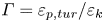 $\varGamma = \varepsilon _{p,tur}/\varepsilon _k$, a common measure of mixing efficiency often assumed to be close to
  $0.2$. Typically,
  $\varepsilon _{p,tur}$ is estimated from microstructure measurements using formulas such as the widely used expression
 \begin{equation} \varepsilon_{p,tur} = \frac{g \alpha \kappa_T\, |\boldsymbol{\nabla} \theta'|^2}{{\rm d}\bar{\theta}/{\rm d}z} \end{equation}
(Oakey Reference Oakey1982; Gargett & Holloway Reference Gargett and Holloway1984), where  $\alpha$ is the thermal expansion coefficient,
  $g$ is the acceleration due to gravity, and
  $\bar {\theta }$ represents the mean potential temperature profile. Consequently,
  $\varepsilon _p$, like the viscous dissipation rate, is generally considered a positive quantity that also converts mechanical energy into BPE or ‘heat’. (For further views on this, see Tailleux Reference Tailleux2009.)
In a double diffusive fluid, double diffusive instabilities can develop even in the absence of mechanical forcing. Within the framework of APE theory, this is possible only if BPE, like APE, can become a source of kinetic energy, and hence if we accept the notion that  $\varepsilon _p$ can become negative. In this paper, we derive a theoretical expression for the ratio
  $\varepsilon _{p}^{dd}/\varepsilon _p^{std}$ of the APE dissipation rates for a double diffusive case over that for a simple fluid. We demonstrate that
  $\varepsilon _p^{dd}$ is negative under the conditions corresponding to the linear stability analysis for both salt finger and diffusive convection regimes. Recently, Middleton & Taylor (Reference Middleton and Taylor2020) proposed to characterise double diffusive instabilities in terms of the sign of the diapycnal component of the molecular buoyancy flux, which is related to the turbulent part
  $\varepsilon _{p,tur}$ of
  $\varepsilon _p$ (equivalently,
  $\varPhi _d$), rather than
  $\varepsilon _p$. However, their criterion succeeds in predicting only the occurrence of the diffusive convection instability, but not the salt finger instability, which suggests that it is the sign of the net APE dissipation rate
  $\varepsilon _{p,lam} + \varepsilon _{p,tur}$ (equivalently
  $\varPhi _d-\varPhi _i$) that represents the most fundamental criterion for double diffusive instabilities. Additionally, we show that considering the APE dissipation rate sheds light on other aspects of double diffusive instabilities in turbulent regimes. For example, it correctly predicts the regime associated with diffusive interleaving in the presence of density-compensated isopycnal gradients of temperature and salinity, which are thought to be essential for the formation of thermohaline staircases (Merryfield Reference Merryfield2000).
The remainder of this paper is organised as follows. Section 2 establishes the general form of the local APE dissipation rate for a double diffusive fluid. Section 3 outlines the conditions necessary for negative APE dissipation. Section 4 provides a comparison of the local and APE frameworks. Section 5 discusses the practical issues related to the computation of the reference temperature and salinity profiles used in our definition of spiciness. Finally, § 6 discusses the results and provides future perspectives.
2. Local APE theory and APE dissipation rate
Similarly to Middleton & Taylor (Reference Middleton and Taylor2020), we study the energetics of double diffusive instabilities for a Boussinesq fluid with a linear equation of state for density governed by the system of equations
 $$\begin{gather} \frac{{\rm D}{\boldsymbol v}}{{\rm D} t} + \frac{1}{\rho_{{\star}}}\,\boldsymbol{\nabla} \delta p ={-} \frac{g\,\delta \rho}{\rho_{{\star}}}\, {\boldsymbol k} + \nu\,\nabla^2 {\boldsymbol v}, \end{gather}$$
 $$\begin{gather}\boldsymbol{\nabla} \boldsymbol{\cdot} {\boldsymbol v} = 0, \end{gather}$$
 $$\begin{gather}\frac{{\rm D}\theta}{{\rm D} t} ={-} \boldsymbol{\nabla} \boldsymbol{\cdot} {\boldsymbol J}_{\theta}, \quad \frac{{\rm D}S}{{\rm D} t} ={-}\boldsymbol{\nabla} \boldsymbol{\cdot} {\boldsymbol J}_S, \end{gather}$$
 $$\begin{gather} \rho = \rho_{{\star}} [ 1 - \alpha (\theta - \theta_{{\star}} ) + \beta (S-S_{{\star}} ) ] , \end{gather}$$
where  $\rho$ is density,
  $p$ is pressure,
  $g$ is gravitational acceleration,
  $S$ is salinity,
  $\theta$ is potential temperature,
  $\alpha$ is the thermal expansion coefficient, and
  $\beta$ is the haline contraction coefficient, while
  $\rho _{\star }$,
  $S_{\star }$ and
  $\theta _{\star }$ are constant reference values for
  $\rho$,
  $S$ and
  $\theta$, respectively. Moreover,
  $\delta p = p-p_0(z)$ and
  $\delta \rho = \rho - \rho _0(z)$ denote the pressure and density anomalies defined relative to the reference pressure and density profiles
  $p_0(z)$ and
  $\rho _0(z) = -g^{-1} \,\textrm {d}p_0/\textrm {d}z$ characterising the Lorenz reference state. Simple diffusive laws are assumed for
  $\theta$ and
  $S$ so that
  ${\boldsymbol J}_{\theta } = -\kappa _T\,\boldsymbol {\nabla } \theta$ and
  ${\boldsymbol J}_s = -\kappa _S\,\boldsymbol {\nabla } S$, where
  $\kappa _T$ and
  $\kappa _S$ are the molecular diffusivities of heat and salt, respectively. The tracer equations (2.3a,b) may be combined with the equation of state (2.4) to form an equation for the Boussinesq buoyancy
  $b_{bou} = g [ \alpha (\theta -\theta _{\star }) - \beta (S-S_{\star })]$,
 \begin{equation} \frac{{\rm D}b_{bou}}{{\rm D} t} ={-} \boldsymbol{\nabla} \boldsymbol{\cdot} {\boldsymbol J}_b, \end{equation}
where
 \begin{equation} {\boldsymbol J}_b = g (\alpha {\boldsymbol J}_{\theta} - \beta {\boldsymbol J}_s ) ={-} g (\kappa_T \alpha\,\boldsymbol{\nabla} \theta - \kappa_S \beta\, \boldsymbol{\nabla} S) \end{equation}
is the molecular buoyancy flux. Note that in the absence of salinity,  ${\boldsymbol J}_b = -\kappa _T\,\boldsymbol {\nabla } b_{bou}$ is down the gradient of the Boussinesq buoyancy, but not in the general case.
To understand how double diffusion affects APE dissipation, the local APE framework (Tailleux Reference Tailleux2013b, Reference Tailleux2018; Novak & Tailleux Reference Novak and Tailleux2018) is preferred over the Winters et al. (Reference Winters, Lombard, Riley and d'Asaro1995) global APE framework used by Middleton & Taylor (Reference Middleton and Taylor2020). Indeed, we show in § 4 that defining the total APE of a fluid as the volume integral of a non-sign definite integrand makes the global APE framework problematic in several respects; for instance, it introduces unphysical terms in its budget. To avoid such difficulties, it is therefore preferable to define the APE of a fluid as the volume integral of the APE density:
 \begin{equation} e_a = e_a(S,\theta,z) ={-} \int_{z_r}^z b(S,\theta,z')\,{\rm d} z', \end{equation}
where  $b(S,\theta,z) = -(g/\rho _{\star }) (\rho (S,\theta )-\rho _0(z))$ is the buoyancy defined relative to Lorenz reference density profile
  $\rho _0(z)$ characterising the notional reference state of minimum potential energy obtainable from the actual state by means of an adiabatic and volume-conserving rearrangement. This definition of buoyancy has the advantage of vanishing in the Lorenz reference state of rest, which is not the case for the Boussinesq buoyancy. To avoid any ambiguity, note that
  $b(S,\theta,z') = -(g/\rho _{\star })(\rho (S(x,y,z,t),\theta (x,y,z,t)) - \rho _0(z'))$ in the integral (2.7), that is, the values of
  $S$ and
  $\theta$ are held constant as the parcel moves from
  $z_r$ to
  $z$, consistent with the idea of an adiabatic and isohaline rearrangement. As is well known, the APE density (2.7) represents the work against buoyancy forces that a parcel needs to counteract to move from its reference position at
  $z_r$, solution of the level of neutral buoyancy equation
 \begin{equation} b(S,\theta,z_r) = 0 ,\end{equation}
to its actual position at  $z$. For simplicity, we disregard the temporal dependence of
  $\rho _0(z)$ as the APE dissipation depends only on spatial gradients of the tracer fields. Inversion of (2.8) establishes that
  $z_r= z_r(\rho ) = z_r(S,\theta )$ is a material function of
  $S$ and
  $\theta$, and is therefore a Lagrangian invariant following fluid parcels in the absence of diffusive sources/sinks of heat and salt.
A local budget equation for the APE density is easily obtained by taking the material derivative of (2.7), which yields
 \begin{align} \frac{{\rm D}e_a}{{\rm D} t} &={-} b\, \frac{{\rm D}z}{{\rm D} t} + \underbrace{b(S,\theta,z_r)}_{{=}0}\, \frac{{\rm D}z_r}{{\rm D} t} - (z-z_r)\,\frac{{\rm D}b_{ou}}{{\rm D} t} \nonumber\\ &={-} b w - \boldsymbol{\nabla} \boldsymbol{\cdot} {\boldsymbol J}_a - \varepsilon_p , \end{align}
where  ${\boldsymbol J}_a$ is the diffusive flux of APE, and
  $\varepsilon _p$ is the APE dissipation rate, given by
 $$\begin{gather} {\boldsymbol J}_a ={-}(z-z_r) {\boldsymbol J}_b, \end{gather}$$
 $$\begin{gather}\varepsilon_p = {\boldsymbol J}_b \boldsymbol{\cdot} \boldsymbol{\nabla} (z-z_r) = \underbrace{- g \left( \alpha \kappa_T\, \frac{\partial \theta}{\partial z} - \beta \kappa_S\,\frac{\partial S}{\partial z} \right)}_{\varepsilon_{p,lam}} + \underbrace{g (\alpha \kappa_T\,\boldsymbol{\nabla} \theta - \beta\,\kappa_S \boldsymbol{\nabla} S ) \boldsymbol{\cdot} \boldsymbol{\nabla} z_r}_{\varepsilon_{p,tur}} . \end{gather}$$
As indicated by (2.11),  $\varepsilon _p$ can be decomposed into ‘laminar’ and ‘turbulent’ components
  $\varepsilon _{p,lam}$ and
  $\varepsilon _{p,tur}$ whose volume integrals
 \begin{equation} \int_{V} \varepsilon_{p,lam}\,\rho_{{\star}}\,{\rm d} V ={-} \varPhi_i, \quad \int_{V} \varepsilon_{p,tur}\,\rho_{{\star}}\,{\rm d} V = \varPhi_d , \end{equation}
can easily be shown to correspond to Winters et al. (Reference Winters, Lombard, Riley and d'Asaro1995) global energy conversions  $-\varPhi _i$ and
  $\varPhi _d$ in the global APE framework. So far, the turbulent mixing community has generally assumed
  $\varPhi _i$ and
  $\varPhi _d$ to represent distinct types of energy conversions, the former with internal energy and the latter with the BPE; however, the analysis of such conversions in real fluids detailed in § 4 clearly indicates that there is no physical basis for such a view, and that in reality,
  $\varepsilon _p$,
  $\varPhi _d$ and
  $\varPhi _i$ all represent conversions with internal energy as established previously by Tailleux (Reference Tailleux2009). In other words,
  $\varepsilon _{p,lam}$ and
  $\varepsilon _{p,tur}$ are parts of the same energy conversion.
Physically, (2.9) states that locally,  $e_a$ can be modified through: (1) conversion with kinetic energy via the buoyancy flux
  $b w$; (2) diffusive and advective transport via
  ${\boldsymbol J}_a$ and advection; (3) ‘dissipation’ that can be occasionally be negative associated with
  $\varepsilon _p$. Physically, our local APE budget (2.9) is simpler in form than that derived previously by Scotti & White (Reference Scotti and White2014) for a single-component fluid, although the two can be verified to be mathematically equivalent. One of the reasons is due to Scotti & White (Reference Scotti and White2014) imposing the diffusive flux of APE density to be down-gradient, namely,
 \begin{equation} {\boldsymbol J}_{a,sw14} ={-}\kappa\,\boldsymbol{\nabla} e_a = \kappa (z-z_r)\,\boldsymbol{\nabla} b_{bou} + \kappa b {\boldsymbol k} = {\boldsymbol J}_a + \kappa b {\boldsymbol k} , \end{equation}
which differs from  ${\boldsymbol J}_a$ by the last term, with the consequence of adding extra terms in their budget equation. Physically, however, the Scotti & White (Reference Scotti and White2014) approach is inconsistent with the analysis of the APE budget for a real fluid (cf. § 4 or Tailleux Reference Tailleux2009), which reveals that decomposing the potential energy into available and unavailable components leads to a decomposition of the heat flux
  ${\boldsymbol J}_q = \varUpsilon {\boldsymbol J}_q + (1-\varUpsilon ) {\boldsymbol J}_q$, with
  $\varUpsilon = (T-T_r)/T$ a Carnot-like thermodynamic efficiency. Physically, it is the first term
  $J_a = \varUpsilon {\boldsymbol J}_q$ that represents the diffusive flux of APE density, whose Boussinesq approximation is given by (2.10). Another reason to be sceptical of (2.13) is that it cannot generalise to the case of a double diffusive two-component fluid, whereas our definition of
  ${\boldsymbol J}_a$ in (2.10) obviously does.
In their study, Middleton & Taylor (Reference Middleton and Taylor2020) derived an expression for the diapycnal component of the buoyancy flux  ${\boldsymbol J}_b\boldsymbol {\cdot } \hat {\boldsymbol n}$ in terms of three parameters – the diffusivity ratio
  $\tau = \kappa _S/\kappa _T$, the gradient ratio
  $G_{\rho } = (\alpha \,|\boldsymbol {\nabla } \theta |)/ (\beta \,|\boldsymbol {\nabla } S|)$ and the angle
  $\gamma$ between
  $\boldsymbol {\nabla } \theta$ and
  $\boldsymbol {\nabla } S$ – such that
  $\cos {\gamma } = \boldsymbol {\nabla } \theta \boldsymbol {\cdot } \boldsymbol {\nabla } S/(|\boldsymbol {\nabla } \theta |\,|\boldsymbol {\nabla } S|)$, with
  $\hat {\boldsymbol n} = \boldsymbol {\nabla } z_r/|\boldsymbol {\nabla } z_r|$, that could similarly be used to study
  $\varepsilon _p$. However, while
  $G_{\rho }$ and
  $\cos {\gamma }$ might be diagnosed easily from the output of a numerical experiment, they cannot be inferred easily from measured oceanic properties, nor are they naturally related to physical parameters known to play a key role in double diffusive instabilities such as density-compensated thermohaline variations. For instance, in the canonical salt finger experiment that they discuss in their § 2.5, Middleton & Taylor (Reference Middleton and Taylor2020) find that
  $\varPhi _d$ becomes negative as the result of the gradients of salinity growing more rapidly than temperature gradients, resulting in the creation of density-compensated thermohaline variations (usually referred to as ‘spice’). In oceanography, the term spice was perhaps first used by Munk (Reference Munk, Wunsch and Warren1981) to quantify the range of possible
  $\theta /S$ behaviour of a seawater sample of given density, from warm and salty (spicy) to fresh and cold (minty). Physically, the creation of spice is of considerable dynamical importance because lateral stirring along isopycnal surfaces is not opposed by restoring buoyancy forces and is therefore considerably more efficient at dissipating tracer variances than vertical stirring. To study the role of spice, Middleton et al. (Reference Middleton, Fine, MacKinnon, Alford and Taylor2021) subsequently reformulated the Middleton & Taylor (Reference Middleton and Taylor2020) expression in terms of the ‘spiciness’ variable
  $\tau = \alpha \theta + \beta S$ (denoted
  $S_p$ in their paper), which may be regarded as the ‘linear’ version of the spiciness variables developed by Jacket & McDougall (Reference Jacket and McDougall1985) or Flament (Reference Flament2002), for instance. Recently, the theory of spiciness was revisited by Tailleux (Reference Tailleux2021), who argued that to be physically meaningful, spice should ideally vanish in a spiceless ocean, and hence that spice variables should be defined as isopycnal anomalies, which is not the case for
  $\tau$ or any related variable. In the present case, this can be implemented in practice by decomposing
  $\theta$ and
  $S$ as
 \begin{equation} \theta = \theta_0 (z_r) + \theta_{\xi} , \quad S = S_0 (z_r) + S_{\xi} , \end{equation}
with the reference profiles  $\theta _0(z_r)$ and
  $S_0(z_r)$ defining the temperature and salinity profiles of the assumed spiceless state, and
  $z_r= z_r(\rho )$ denoting the reference position of a fluid parcel as before. Provided that
  $\theta _0(z_r)$ and
  $S_0(z_r)$ are defined as the (thickness-weighted) isopycnal mean temperature and salinity, respectively, they contain all necessary information to compute density
  $\rho =\rho _{\star }[1-\alpha (\theta _0(z_r)-\theta _{\star }) - \beta (S_0(z_r)-S_{\star })]$, thus allowing them to be interpreted as the ‘active’ components of
  $\theta$ and
  $S$. In contrast, the isopycnal anomalies
  $\theta _{\xi }$ and
  $S_{\xi }$ are density-compensated
  $\alpha \theta _{\xi } = \beta S_{\xi }$ and therefore do not contribute to density, thus allowing them to be interpreted as the passive components of
  $\theta$ and
  $S$. Physically, defining the spiceless stratification
  $\theta _0(z),S_0(z)$ in terms of thickness-weighted isopycnal means can be justified on the grounds that such a state is the one that would be expected to result in the idealised limit of infinitely fast (resp. infinitely slow) isopycnal (resp. diapycnal) mixing. How to estimate these in practice are discussed in § 5. As shown below, defining spiciness in this way allows us to define a new set of parameters with which to study the behaviour of
  $\varepsilon _p$, different from those used by Middleton & Taylor (Reference Middleton and Taylor2020) and Middleton et al. (Reference Middleton, Fine, MacKinnon, Alford and Taylor2021), and which we consider to be more physical and more relevant.
In the following,  $S_{\xi }$ and
  $\theta _{\xi }$ are combined into the variable
  $\xi = \rho _{\star } ( \alpha \theta _{\xi } + \beta S_{\xi }$) to define a single measure of spiciness having the dimension of density, as is commonly done in the literature. After some manipulation, it is possible to rewrite
  $\varepsilon _p$ in the form
 \begin{align}\varepsilon_p &= g \left(
\kappa_T \alpha\, \frac{\partial \tilde{\theta}}{\partial
z_r} - \kappa_S \beta\,\frac{\partial \tilde{S}}{\partial
z_r} \right) \left( |\boldsymbol{\nabla} z_r|^2 -
\frac{\partial z_r}{\partial z} \right) + \frac{g (
\kappa_T - \kappa_S )}{2\rho_{{\star}}} \left(
\boldsymbol{\nabla} z_r\boldsymbol{\cdot}
\boldsymbol{\nabla} \xi - \frac{\partial \xi}{\partial z}
\right) \nonumber\\ &= K_{v0}\, N_0^2(z_r) \left[
\frac{R_{\rho} - \tau }{R_{\rho}-1} + (1-\tau )
{\mathcal{M}} \right]\left( 1 - \frac{\partial_z
z_r}{|\boldsymbol{\nabla} z_r|^2} \right),\end{align}
\begin{align}\varepsilon_p &= g \left(
\kappa_T \alpha\, \frac{\partial \tilde{\theta}}{\partial
z_r} - \kappa_S \beta\,\frac{\partial \tilde{S}}{\partial
z_r} \right) \left( |\boldsymbol{\nabla} z_r|^2 -
\frac{\partial z_r}{\partial z} \right) + \frac{g (
\kappa_T - \kappa_S )}{2\rho_{{\star}}} \left(
\boldsymbol{\nabla} z_r\boldsymbol{\cdot}
\boldsymbol{\nabla} \xi - \frac{\partial \xi}{\partial z}
\right) \nonumber\\ &= K_{v0}\, N_0^2(z_r) \left[
\frac{R_{\rho} - \tau }{R_{\rho}-1} + (1-\tau )
{\mathcal{M}} \right]\left( 1 - \frac{\partial_z
z_r}{|\boldsymbol{\nabla} z_r|^2} \right),\end{align}
which depends on the parameters
 \begin{equation} \left.\begin{array}{c} \displaystyle {\mathcal{M}} \equiv \dfrac{g}{2\rho_{{\star}}\, N_0^2(z_r)}\dfrac{\boldsymbol{\nabla} z_r\boldsymbol{\cdot} \boldsymbol{\nabla} \xi -\partial_z \xi}{|\boldsymbol{\nabla} z_r|^2 -\partial_z z_r} \quad (\text{spiciness parameter}), \\ \displaystyle K_{v0} \equiv \kappa_T\,|\boldsymbol{\nabla} z_r|^2 = \kappa_T \left( \dfrac{{\rm d} \rho_0}{\partial z_r}(z_r) \right)^{{-}2} |\boldsymbol{\nabla} \rho|^2 \quad (\text{effective diffusivity}), \\ \displaystyle N_0^2 (z_r) \equiv{-}\dfrac{g}{\rho_{{\star}}}\, \dfrac{{\rm d} \rho_0}{{\rm d} z_r}(z_r) = g \left( \alpha\,\dfrac{{\rm d} \theta_0}{{\rm d} z_r} - \beta\,\dfrac{{\rm d} S_0}{{\rm d} z_r} \right) (z_r) \quad (\text{reference }\ N^2), \\ \displaystyle R_{\rho} \equiv R_{\rho}(z_r) = \left. \alpha\,\dfrac{{\rm d} \theta_0}{{\rm d} z_r} \right/ \beta\,\dfrac{{\rm d} S_0}{{\rm d} z_r} \quad (\text{density ratio}), \\ \displaystyle \tau \equiv \dfrac{\kappa_S}{\kappa_T} \quad (\text{diffusivity ratio}). \end{array}\right\}\end{equation}
Our choices of control parameters  $R_{\rho }$ and
  ${\mathcal {M}}$ differ from those of Middleton & Taylor (Reference Middleton and Taylor2020), who chose the gradient ratio
  $G_{\rho } \equiv \alpha \,|\boldsymbol {\nabla } \theta |/(\beta \,|\boldsymbol {\nabla } S|)$, and the angle
  $\phi$ between
  $\boldsymbol {\nabla } \theta$ and
  $\boldsymbol {\nabla } S$ defined by
  $\cos {\phi } = -\boldsymbol {\nabla } \theta \boldsymbol {\cdot } \boldsymbol {\nabla } S/(|\boldsymbol {\nabla } \theta |\,|\boldsymbol {\nabla } S|)$ instead. The present approach is preferred here because
  $R_{\rho }$ is a more commonly encountered parameter in the literature, while
  ${\mathcal {M}}$ is more naturally connected to the physics of lateral thermohaline intrusions, whose importance is well established. Moreover,
  $K_{v0}$ represents a local version of the effective diffusivity concept originally proposed by Winters & D'Asaro (Reference Winters and D'Asaro1996) and Nakamura (Reference Nakamura1996) based on thermal diffusion, and is positive definite by construction. Also,
  $K_{v0}$ is different from the effective diffusivity
  $K_{eff}$ introduced in § 5 and governing the evolution of the sorted density profile. Note that although the term within square brackets in (2.15) goes to infinity as
  $R_{\rho } \rightarrow 1$,
  $\varepsilon _p$ remains finite as
  $N_0^2 \rightarrow 0$.
3. APE dissipation and diffusive stability
3.1. Single-component fluid
Even in the case of a single component fluid, the APE dissipation rate  $\varepsilon _p$, unlike the viscous dissipation rate
  $\varepsilon _k$, is not guaranteed to be always positive definite. To see this, let us first set
  ${\mathcal {M}}=0$ and
  $\tau =1$ in (2.15), leading to
 \begin{equation} \varepsilon_p \equiv \varepsilon_p^{std} = K_{v0}\,N_0^2(z_r) \left( 1 - \frac{\partial_z z_r}{|\boldsymbol{\nabla} z_r|^2} \right) = \kappa_T \left( |\boldsymbol{\nabla} z_r|^2 - \frac{\partial z_r}{\partial z} \right) N_0^2 .\end{equation}
Since  $\kappa _T$ and
  $N_0^2$ are positive by construction, (3.1) shows that
  $\varepsilon _p$ can occasionally be negative provided that
 \begin{equation} {\mathcal{F}} \equiv |\boldsymbol{\nabla} z_r|^2 - \frac{\partial z_r}{\partial z} = |\nabla_h z_r|^2 + \left( \frac{\partial z_r}{\partial z} \right)^2 - \frac{\partial z_r}{\partial z} < 0 , \end{equation}
where  $\nabla _h$ denotes the horizontal gradient. If viewed as a quadratic polynomial in
  $\partial z_r/\partial z$ with discriminant
  $\varDelta = 1 - 4\,|\nabla _h z_r|^2$,
  ${\mathcal {F}}$ can be negative only when possessing two real roots, that is, when
  $\varDelta <0$, or equivalently when
 \begin{equation} |\nabla_h z_r| < \tfrac{1}{2} .\end{equation}
In that case,  ${\mathcal {F}}$ and
  $\varepsilon _p^{std}$ achieve their maximally negative values for
  $\partial z_r/\partial z = 1/2$:
 \begin{equation} | \varepsilon_{p,min}^{std} | = \kappa_T N_0^2 \left( \frac{1}{4} - |\nabla_h z_r|^2 \right) < \frac{\kappa_T N_0^2}{4} , \end{equation}
which is bounded above by  $\kappa _T N_0^2/4$, which is laminar-like in character and therefore extremely small relative to turbulent values. Nevertheless, because a negative
  $\varepsilon _p$ can potentially cause perturbations to grow with time, it seems of interest to estimate the time scale
  $\tau _{APE} = e_a/\varepsilon _p$ of the latter. Using the fact that the APE density scales as
  $N_0^2 \zeta ^2/2$, where
  $\zeta = z-z_r$, this leads to
 \begin{equation} \tau_{APE} = \frac{N_0^2\zeta^2/2}{\kappa_T N_0^2/4} = \frac{2 \zeta^2}{\kappa_T}.\end{equation}
For illustration, using  $\kappa _T = 10^{-7} \textrm {m}^2\ \textrm {s}^{-1}$ and
  $\zeta = 1 \ \textrm {cm} = 10^{-2}\ \textrm {m}$ yields
  $\tau = 2 \times 10^{-4}/10^{-7} = 2 \times 10^3\ \textrm {s} \approx 33 \ \textrm {min}$, which is fast enough to be observable in the laboratory, at least in principle. Inequality (3.3), which may be rewritten as
  $|\nabla _h \zeta | <1/2$, also requires that the horizontal scales of the unstable perturbations be larger than their vertical scales. A priori, perturbations with the required characteristics cannot occur spontaneously; they can only be created with some form of appropriate gentle mechanical stirring. These considerations appear to be consistent with the experimental observation of steps formation by Park, Whitehead & Gnanadesikan (Reference Park, Whitehead and Gnanadesikan1994), who observed the smaller steps to grow faster than larger ones. However, these conclusions are only speculative at this stage, and more research is needed to confirm or disprove the relevance of our results.
3.2. Binary fluid: spiceless case  ${\mathcal {M}}=0$

In the double diffusive case but in the absence of spiciness, (2.15) reduces to
 \begin{equation} \varepsilon_p = K_{v0}\,N_0^2 (z_r) \left( \frac{R_{\rho} - \tau }{R_{\rho} - 1 } \right) \left( 1 - \frac{\partial_z z_r}{|\boldsymbol{\nabla} z_r|^2} \right) . \end{equation}
This time, the sign of  $\varepsilon _p$ is controlled by the sign of the product of
  ${\mathcal {F}}$ times the density-ratio-dependent term within parentheses. Restricting attention to the case
  $\tau <1$ pertaining to thermosolutal convection, table 1 shows that
  $\varepsilon _p$ can be negative for all possible values of
  $R_{\rho }$, although not necessarily in both laminar and turbulent regimes.
Table 1. Sign of the APE dissipation rate  $\varepsilon _p$ as a function of the density ratio
  $R_{\rho }$ and the sign of
  ${\mathcal {F}} = |\boldsymbol {\nabla } z_r|^2 - \partial _z z_r$ in the absence of spiciness (
 ${\mathcal {M}}=0)$, in the case where
  $\tau = \kappa _S/\kappa _T<1$, characteristic of salty water.

3.2.1. Diffusive convection: $\tau < R_{\rho } < 1$

In this case,  $\varepsilon _p$ is negative only if
  ${\mathcal {F}}>0$, in which case the diapycnal component of the buoyancy flux is associated with up-gradient diffusion, as shown by Middleton & Taylor (Reference Middleton and Taylor2020). Note that the range
  $\tau < R_{\rho } < 1$ is associated with diffusive convection instability only for inviscid flows. In reality, stability analysis shows that viscosity restricts the range of instabilities to the range
 \begin{equation} \frac{Pr + \tau}{Pr + 1} < R_{\rho} < 1 ,\end{equation}
where  $Pr = \nu /\kappa _T$ is the Prandtl number, with
  $\nu$ the molecular viscosity. For typical oceanic conditions,
  $\tau \approx 0.01$ and
  ${Pr} \approx 7$ yield the restricted range
  $0.876 < R_{\rho }<1$.
3.2.2. ‘Salt’ finger instability: $R_{\rho }>1$

According to classical linear stability analysis, salt fingers are expected to develop in the density ratio range
 \begin{equation} 1 < R_{\rho} < \frac{1}{\tau} \end{equation}
(e.g. Radko Reference Radko2013). In that range, table 1 shows that APE dissipation can be negative only if  ${\mathcal {F}}<0$, and hence that the appropriate expression for
  $\varepsilon _p$ is
 \begin{equation} \varepsilon_p = \kappa_T N_0^2 \left( |\boldsymbol{\nabla} z_r|^2 - \frac{\partial z_r}{\partial z}\right) \left( \frac{R_{\rho} - \tau}{R_{\rho}-1} \right) = \kappa_T N_0^2 {\mathcal{F}} \left( \frac{R_{\rho}-\tau}{R_{\rho}-1} \right) .\end{equation}
Equation (3.9) shows that negative APE dissipation in that case corresponds to the amplification of the negative APE dissipation in a single-component fluid multiplied by the amplification factor
 \begin{equation} \frac{R_{\rho}-\tau}{R_{\rho}-1} > 1 .\end{equation}
Since the time scale for the growth of an unstable perturbation is a priori inversely proportional to  $\varepsilon _p$, the expectation is that the same perturbations in single-component and double diffusive fluids will grow faster in the former than in the latter. A key difference, however, is that in a double diffusive fluid, diffusive instabilities are able to grow spontaneously, whereas in a single-component fluid, their development requires initiation by means of external mechanical stirring of the right kind.
Since  ${\mathcal {F}}$ can be negative only for laminar-like conditions, it follows that density-compensated thermohaline variations need to develop in order for the APE dissipation to remain negative as the flow transitions to turbulence. In fact, this is precisely what appears to happen in the salt finger experiments of Middleton & Taylor (Reference Middleton and Taylor2020), and as was previously advocated by Merryfield (Reference Merryfield2000).
3.3. Impact of spiciness anomalies on diffusive instability
Density-compensated thermohaline variations are a characteristic feature of ocean stratification in all regions and at all depths (Tailleux Reference Tailleux2021). Consequently, spiciness and a non-zero value of  ${\mathcal {M}}$ are likely to be representative of the general situation. Assuming a prevalence of the turbulent regime, we can make the approximation
  $1 - \partial _z z_r/|\boldsymbol {\nabla } z_r|^2 \approx 1$, and the relevant expression for
  $\varepsilon _p$ in the oceanic case appears as
 \begin{equation} \varepsilon_p = K_{v0}\,N_0^2(z_r) \left [ \frac{R_{\rho} - \tau }{R_{\rho}-1} + (1-\tau ) {\mathcal{M}} \right ] .\end{equation}
 This equation shows that the single-component APE dissipation rate  $\varepsilon _p^{std} = K_{v0} N_0^2(z_r)$ is modulated by the factor
 \begin{equation} f(R_{\rho},\tau,{\mathcal{M}}) = \frac{R_{\rho}-\tau}{R_{\rho}-1} + (1-\tau) {\mathcal{M}} . \end{equation}
 To illustrate the effect of this factor, figure 1 depicts  $f(R_{\rho },\tau,{\mathcal {M}})$ as a function of
  $R_{\rho }$ and
  ${\mathcal {M}}$ for
  $\tau = \kappa _S/\kappa _T = 0.01$. A notable difference from the spiceless case is the possibility of negative
  $\varepsilon _p$ for a wide range of stratification, depending on the values of
  ${\mathcal {M}}$:
 \begin{equation} {\mathcal{M}} <{-} \frac{1}{1-\tau}\,\frac{R_{\rho}-\tau}{R_{\rho}-1} . \end{equation}
Figure 1. The amplification factor  $f(R_{\rho },\tau,{\mathcal {M}})$ (given by (3.12)) as a function of the spiciness parameter
  ${\mathcal {M}}$ and density ratio
  $R_{\rho }$, for
  $\tau =0.01$.
This opens up various scenarios, ranging from complete inhibition of mixing ( $\,f = 0$) to enhanced mixing (
 $\,f > 1$) and even diffusive instability (
 $\,f < 0$). In the turbulent case, the value of
  ${\mathcal {M}}$ approximates to
 \begin{equation} {\mathcal{M}} = \frac{g}{2 \rho_{{\star}} N_0^2}\, \frac{\boldsymbol{\nabla} z_r\boldsymbol{\cdot} \boldsymbol{\nabla} \xi - \partial_z \xi}{|\boldsymbol{\nabla} z_r|^2 - \partial_z z_r} \approx \frac{g}{2\rho_{{\star}} N_0^2}\,\frac{\boldsymbol{\nabla} z_r\boldsymbol{\cdot} \boldsymbol{\nabla} \xi}{|\boldsymbol{\nabla} z_r|^2} ={-} \frac{\boldsymbol{\nabla} \xi \boldsymbol{\cdot} \boldsymbol{\nabla} \rho}{2\,|\boldsymbol{\nabla} \rho|^2} . \end{equation}
 This reveals that for  ${\mathcal {M}}$ to be negative, spiciness and density gradients need to be positively correlated. Exploring the possibility and magnitude of such a situation requires a way to express in terms of the large-scale gradients of
  $\xi$ and
  $\rho$, which warrants further investigation beyond the scope of this study.
4. Comparison of APE frameworks
Holliday & McIntyre (Reference Holliday and McIntyre1981) and Andrews (Reference Andrews1981) had already shown the possibility of building Lorenz APE theory from a local principle by the time Winters et al. (Reference Winters, Lombard, Riley and d'Asaro1995) published their study in the mid-1990s. However, the local APE framework was still rudimentary and had not been used for any concrete applications. This situation has improved in recent years, as the local APE framework has progressed rapidly and achieved full maturity, being able to deal with a fully compressible multi-component stratified fluid (Tailleux Reference Tailleux2018). In this paper, we prefer the local APE framework to the global APE framework, because it is objectively simpler and more physical, even though this is not necessarily widely appreciated or acknowledged. This section intends to reveal some of the unphysical aspects of the global APE framework that are commonly overlooked, but easily uncovered by the local APE framework.
We start by reviewing the main results of the global APE framework as first derived by Winters et al. (Reference Winters, Lombard, Riley and d'Asaro1995). Following Lorenz (Reference Lorenz1955), Winters et al. (Reference Winters, Lombard, Riley and d'Asaro1995) (indicated by ‘ $W95$’ in equations) defined the APE of a fluid as the potential energy of the actual state minus that of the adiabatically sorted state, i.e.
 \begin{equation} E_a^{W95} = \int_{V} \rho g z \,{\rm d} V - \int_{V} \rho_r g z_r\,{\rm d} V = \int_{V}\rho g (z-z_r) \,{\rm d} V, \end{equation}
and showed that its budget equation may be written in the form
 \begin{equation} \frac{{\rm d} E_a^{W95}}{{\rm d} t} = \underbrace{\int_{V} \rho g w \,{\rm d} V}_{\varPhi_z} \underbrace{{}- g \oint_{S} (z\rho -\psi) {\boldsymbol v}\boldsymbol{\cdot} {\boldsymbol n}\, {\rm d} S}_{S_{APE}^{adv}} + \underbrace{\kappa g \oint_{S} (z - z_r)\,\boldsymbol{\nabla} \rho \boldsymbol{\cdot} {\boldsymbol n} \,{\rm d} S}_{S_{APE}^{diff}} - (\varPhi_d-\varPhi_i),\end{equation}
where  $\varPhi _z$ represents the conversion with kinetic energy,
  $S_{APE}^{adv}$ represents the advective flux of APE through the boundaries enclosing the control volume considered, and
  $S_{APE}^{diff}$ represents the diffusive flux of APE through the same boundaries. The expressions for
  $\varPhi _i$ and
  $\varPhi _d$ are given by
 $$\begin{gather} \varPhi_i ={-}\kappa g A (\bar{\rho}_{top} - \bar{\rho}_{bottom}), \end{gather}$$
 $$\begin{gather}\varPhi_d ={-} \kappa g \int_{V} \frac{\partial z_r}{\partial \rho}\,|\boldsymbol{\nabla} \rho |^2 \,{\rm d} V, \end{gather}$$
where  $A$ is the cross-section of the domain, assumed constant and the overbar denotes surface average, while the quantity
  $\psi$ entering the expression for the advective flux is given by
 \begin{equation} \psi = \int^{\rho} z_r(\tilde{\rho},t) \,{\rm d} \tilde{\rho} . \end{equation}
For the most part, the derivation of (4.2) is straightforward, except for the demonstration that
 \begin{equation} \int_{V} \rho g\,\frac{\partial z_r}{\partial t} \,{\rm d} V = 0, \end{equation}
which is non-trivial. A key point of this paper concerns the proper interpretation of  $\varPhi _i$ and
  $\varPhi _d$. Following Winters et al. (Reference Winters, Lombard, Riley and d'Asaro1995),
  $\varPhi _d$ and
  $\varPhi _i$ have been interpreted as representing two different types of energy conversion, with BPE and internal energy, respectively. The need for revisiting this interpretation is explained below.
The global APE budget (4.2) is now compared with that obtained by integrating the local APE density budget. This is done here for a two-constituent fluid with time-dependent Lorenz reference state, for which the local APE density takes the form
 \begin{equation} e_a = e_a(S,\theta,z,t) ={-}\int_{z_r}^z b(S,\theta,\tilde{z},t)\,{\rm d} \tilde{z} = \frac{g}{\rho_{{\star}}} \int_{z_r}^z [ \rho(S,\theta) - \rho_0(\tilde{z},t) ] \,{\rm d} \tilde{z} , \end{equation}
with the global APE being now defined as the volume-integrated APE density
 \begin{equation} E_a = \int_{V} \rho_{{\star}} e_a \,{\rm d} V . \end{equation}
Because (4.7) implies that  $\rho _{\star } e_a = \rho g (z-z_r) + p_0(z,t) - p_0(z_r,t)$, it follows that
  $E_a$ can be regarded as the sum of
  $E_a^{W95}$ plus an additional term related to the work against the vertical reference pressure gradient, as
 \begin{equation} E_a = E_a^{W95} + \int_{V} [ p_0(z,t) - p_0(z_r,t) ] \,{\rm d} V.\end{equation}
Equation (4.9) shows that the validity of the global definition of APE  $E_a^{W95}$ requires the second term pertaining to the work against the reference pressure gradient to vanish. This is easily verified to be the case if the volume
  $V$ enclosing the fluid remains unchanged under the isochoric adiabatic rearrangement
  ${\boldsymbol x} \rightarrow {\boldsymbol x}_r$ used to construct
  $\rho _0(z,t)$, as then
  $\partial (x,y,z)/\partial (x_r,y_r,z_r) = 1$,
  $\textrm {d} V = \textrm {d} V_r$,
  $V_r = V$, thus ensuring that
 \begin{equation} \int_{V} p_0(z_r,t) \,{\rm d} V = \int_{V_r} p_0(z_r) \,{\rm d} V_r = \int_{V} p_0(z,t) \, {\rm d} V , \end{equation}
as requested (e.g. Roullet & Klein Reference Roullet and Klein2009; Tailleux Reference Tailleux2013b; Winters & Barkan Reference Winters and Barkan2013). However, the identity  $E_a = E_a^{W95}$ is not expected to necessarily hold for more complex situations, although the precise circumstances under which this happens have yet to be fully understood and discussed in the literature.
For a time-dependent Lorenz reference state, the local APE budget (2.9) derived earlier is easily shown to be given by
 \begin{equation} \frac{\partial e_a}{\partial t} ={-} {\boldsymbol v}\boldsymbol{\cdot} \boldsymbol{\nabla} e_a - b w - \boldsymbol{\nabla} \boldsymbol{\cdot} {\boldsymbol J}_a - \varepsilon_p - \frac{g}{\rho_{{\star}}} \int_{z_r}^z \frac{\partial \rho_0}{\partial t} (\tilde{z},t) \,{\rm d} \tilde{z},\end{equation}
where  ${\boldsymbol J}_a = -(z-z_r){\boldsymbol J}_b$ and
  $\varepsilon _p = {\boldsymbol J}_b \boldsymbol {\cdot } \boldsymbol {\nabla } (z-z_r)$ as before. By taking the volume integral of (4.11), the evolution equation for the global APE
  $E_a$ is easily shown to be
 \begin{equation} \frac{{\rm d} E_a}{{\rm d} t} =\underbrace{-\int_{V} \rho_{{\star}} b w \,{\rm d} V}_{-\varPhi_z} \underbrace{{}- \oint_{S} \rho_{{\star}} e_a {\boldsymbol v} \boldsymbol{\cdot} {\boldsymbol n}\, {\rm d} S}_{S_{APE}^{adv}} + \underbrace{\oint_{S} \rho_{{\star}} (z-z_r) {\boldsymbol J}_b \boldsymbol{\cdot} {\boldsymbol n}\,{\rm d} S}_{S_{APE}^{diff}} -\underbrace{\int_{V} \rho_{{\star}} \varepsilon_p \,{\rm d} V}_{\varPhi_d-\varPhi_i} ,\end{equation}
where the expressions for  $\varPhi _i$ and
  $\varPhi _d$ are
 \begin{align} \varPhi_i &={-} \int_{V} \rho_{{\star}} \varepsilon_{p,lam}\,{\rm d}V = \rho_{{\star}} g A [ \alpha \kappa_T\,{\rm \Delta} \theta - \beta \kappa_S\,{\rm \Delta} S ] \nonumber\\ &= \rho_{{\star}} g A \kappa_T \beta\,{\rm \Delta} S \left [ \frac{\alpha\,{\rm \Delta} \theta}{\beta\, {\rm \Delta} S} - \frac{\kappa_S}{\kappa_T} \right ] = \rho_{{\star}} g A \kappa_T \beta\,{\rm \Delta} S\, ( R_{\rho}^{bulk} - \tau ), \end{align}
 \begin{align} \varPhi_d &= \int_{V} \rho_{{\star}} \varepsilon_{p,tur}\,{\rm d}V = \int_{V} g (\alpha \kappa_T\,\boldsymbol{\nabla} \theta - \beta \kappa_S\,\boldsymbol{\nabla} S ) \boldsymbol{\cdot} \boldsymbol{\nabla} z_r\rho_{{\star}} \,{\rm d} V, \end{align}
where  ${\rm \Delta} \theta = \bar {\theta }_{top} - \bar {\theta }_{bottom}$, and
  ${\rm \Delta} S = \bar {S} _{top} - \bar {S}_{bottom}$, while
  $R_{\rho }^{bulk}$ is a bulk density ratio. For canonical salt finger instability,
  $1< R_{\rho }^{bulk} < 1/\tau$, in which case (4.13) predicts
  $\varPhi _i>0$ as required to act as a source of APE. Note that the last term in (4.11) may be written in the form
  $F(z,t)-F(z_r,t)$, with
  $F$ such that
  $(\partial F/\partial z)(z,t) = (\partial \rho _0/\partial t)(z,t)$. As a result, its volume integral must vanish whenever the second term of (4.9) also vanishes for the same reason, as explained above.
Winters & Barkan (Reference Winters and Barkan2013) assumed that when  $E_a$ equals
  $E_a^{W95}$, their respective budgets should be equivalent and described by the equations for an open domain derived previously by Winters et al. (Reference Winters, Lombard, Riley and d'Asaro1995). We disagree with this view, however, because the budgets of
  $E_a$ and
  $E_a^{W95}$ are closely related to the local budgets of their integrands, but these are not equivalent, as established above. Physically, the non-equivalence of the budgets for
  $E_a$ and
  $E_a^{W95}$ is due to the integrand of
  $E_a^{W95}$ lacking a vital piece of information about the energetics of stratified fluids compared to
  $E_a$, namely the fact that when a fluid parcel moves from its reference position
  $z_r$ to its actual position, it has to work not only against gravity, but also against the vertical reference pressure gradient. More generally, Tailleux (Reference Tailleux2013b) shows that work against buoyancy forces actually involves three terms: (1) one associated with changes in gravitational potential energy; (2) one associated with changes in internal energy; and (3) one associated with work against the reference pressure gradient. Even if the latter term integrates to zero over the whole fluid domain, it is still necessary to retain it for correctly predicting the advective flux of APE through the boundaries of open domains. Two key differences characterise the non-equivalence of the budgets for
  $E_a$ and
  $E_a^{W95}$: (1) in Winters et al. (Reference Winters, Lombard, Riley and d'Asaro1995), the reversible conversion with kinetic energy
  $\varPhi _z$ is associated with the density flux
  $\rho g w$, but with the buoyancy flux
  $-b w$ in the local APE framework; (2) in Winters et al. (Reference Winters, Lombard, Riley and d'Asaro1995), the advective flux of APE through boundaries
  $S_{APE}^{adv}$ is associated with the flux of the bizarre quantity
  $g (z\rho -\psi )$ but with the flux of APE density
  $e_a$ in the local framework, which makes much more sense. The unphysical character of the advective flux of APE in Winters et al. (Reference Winters, Lombard, Riley and d'Asaro1995) highlights the well-known problematic character of the global APE framework for regional studies, which was one of the key motivations for the quest of a local available energy framework (Tailleux Reference Tailleux2013a).
The unphysical character of the advective flux of APE in the Winters et al. (Reference Winters, Lombard, Riley and d'Asaro1995) global APE budget for open domains is problematic and can be corrected only by using the local APE framework. The issue is vital, because recent studies of local energetics have demonstrated the key importance of the lateral advection of APE density for understanding important physical processes, such as storm track dynamics (Novak & Tailleux Reference Novak and Tailleux2018; Federer et al. Reference Federer, Papritz, Sprenger, Grams and Wenta2024), tropical cyclone intensification (Harris et al. Reference Harris, Tailleux, Holloway and Vidale2022), or the energetics of the thermohaline circulation (Gregory & Tailleux Reference Gregory and Tailleux2011; Sijp et al. Reference Sijp, Gregory, Tailleux and Spence2012). Importantly, it is worth noting that  $E_a$ and
  $E_a^{W95}$ are also non-equivalent numerically. Indeed, in the global framework, the APE of the fluid is estimated as a small residual between two very large terms, which is ill-conditioned and prone to large numerical errors. In the local framework, however, the APE of a fluid is estimated as the sum of small non-negative numbers, which is numerically robust and very accurate. As a result, the field would benefit greatly from switching to the local APE framework, as this is the better and more physical-based practice.
5. Reference state variables
The practical implementation of the above theoretical results requires the computation of the Lorenz reference density profile  $\rho _0(z,t)$, as well as of the associated isopycnal temperature and salinity averages necessary for defining spiciness. Here, we provide the mathematical foundations for defining the latter in terms of probability density functions (p.d.f.s), which allows one to compute these in practice without the use of sorting. These results pertain to arbitrary domains and unify the p.d.f. approaches of Tseng & Ferziger (Reference Tseng and Ferziger2001) and Saenz et al. (Reference Saenz, Tailleux, Butler, Hughes and Oliver2015), while also making use of previous ideas by Hochet & Tailleux (Reference Hochet and Tailleux2019) and Hochet et al. (Reference Hochet, Tailleux, Kuhlbrodt and Ferreira2021).
5.1. Reference position $z_r(\rho,t)$ and density profile $\rho _0(z,t)$


The classical interpretation of the Lorenz reference state as an isochoric rearrangement of fluid parcels is easy to understand and implement algorithmically. However, it does not easily lend itself to mathematical analysis. Here, we derive expressions for defining and constructing the Lorenz reference density profile  $\rho _0(z,t)$ and its inverse function
  $z_r(\rho,t)$ (such that
  $\rho _0(z_r(\rho,t),t) = \rho$ at all times) in a way that greatly facilitates the study of its mathematical properties. Our approach is not entirely new, as elements of it can be found in Winters et al. (Reference Winters, Lombard, Riley and d'Asaro1995) or in the p.d.f. approaches of Tseng & Ferziger (Reference Tseng and Ferziger2001), Saenz et al. (Reference Saenz, Tailleux, Butler, Hughes and Oliver2015), Hochet & Tailleux (Reference Hochet and Tailleux2019), Hochet et al. (Reference Hochet, Tailleux, Kuhlbrodt and Ferreira2021) and Penney et al. (Reference Penney, Morel, Haynes, Auclair and Nguyen2020), but is useful to introduce the approaches discussed next. To that end, let us assume that the domain containing the fluid is bounded at the top by a rigid lid at
  $z=0$, and at its bottom by a spatially varying bottom topography at
  $z=-H(x,y)$. We denote by
  $\hat {V}(z)$ the volume between an arbitrary depth
  $z$ and the surface, and by
  $A(z) = -\textrm {d} V(z)/\textrm {d} z$ the cross-sectional area of the domain at depth
  $z$.
$z$.
Physically, the reference depth  $z = z_r(\rho,t)$ of a fluid parcel must be such that the volume of water between
  $z_r(\rho,t)$ and the surface, namely,
 \begin{equation} \hat{V}(z_r) = \int_{z_r}^0 A(z)\,{\rm d} z, \end{equation}
must equal the volume of water in physical space made up of all the fluid parcels of densities less than  $\rho$, namely,
 \begin{equation} V(\rho,t) = \int_{V(\rho({\boldsymbol x}',t) \le \rho)}\, {\rm d} V' = \int_{V} H(\rho - \rho({\boldsymbol x}',t)) \,{\rm d} V', \end{equation}
where  $H$ denotes the Heaviside step function defined as in Winters et al. (Reference Winters, Lombard, Riley and d'Asaro1995):
 \begin{equation} H(\rho({\boldsymbol x},t) - \rho({\boldsymbol x}_0,t)) = \begin{cases} 0, & \rho ({\boldsymbol x},t) < \rho({\boldsymbol x}_0,t),\\[3pt] \dfrac{1}{2}, & \rho({\boldsymbol x},t) = \rho({\boldsymbol x}_0,t), \\[3pt] 1, & \rho({\boldsymbol x},t) > \rho({\boldsymbol x}_0,t). \end{cases}\end{equation}
Equating the two volumes  $\hat {V}(z_r) = V(\rho,t)$ yields an implicit equation for
  $z_r(\rho,t)$, which may be inverted to yield
 \begin{equation} z_r(\rho,t) = \hat{V}^{{-}1}[V(\rho,t)] ,\end{equation}
which in the case where  $A(z) = \textrm {constant}$, reduces to
 \begin{equation} z_r(\rho,t) ={-}\frac{V(\rho,t)}{A}, \end{equation}
as derived previously by Winters et al. (Reference Winters, Lombard, Riley and d'Asaro1995). As an illustration, figure 2(a) shows the constant Lorenz reference depth  $z_r(\rho,t) = -1000\ \textrm {m}$ for a realistic ocean, with figure 2(b) showing the corresponding position in reference state space. Construction of the Lorenz reference state for a realistic ocean has been discussed in Saenz et al. (Reference Saenz, Tailleux, Butler, Hughes and Oliver2015) and Tailleux (Reference Tailleux2016, Reference Tailleux2021). Once
  $z_r(\rho,t)$ has been determined for a number of target densities, the reference density profile
  $\rho _0(z,t)$ may be obtained simply by solving the implicit relation
  $\rho _0(z_r(\rho,t),t) = \rho$ at a number of discrete reference depths, from which an interpolator may be constructed to infer the reference density for other values. Alternatively, using the fact that
  $\rho = \rho _0(z_r,t)$ by definition, one may also solve the equation
  $\hat {V}(z_r) = V(\rho,t)$ in the form
  $\hat {V}(z_r) = V(\rho _0(z_r,t),t)$ to infer
  $\rho _0(z_r,t)$ at a number of predetermined target reference depths.

Figure 2. Mapping of (a) physical space onto (b) reference state space.
Note that by differentiating the equality  $\hat {V}(z_r) = V(\rho,t) = V(\rho _0(z_r,t),t)$ with respect to
  $z_r$, the following useful expression for
  $\partial \rho _0/\partial z_r$ may be obtained:
 \begin{equation} \frac{\partial \rho_0}{\partial z}(z_r,t) ={-}\left(\frac{\partial V}{\partial \rho} \right) ^{{-}1} A(z_r) .\end{equation}
The above expressions establish that the practical computation of  $z_r(\rho,t)$ and
  $\rho _0(z,t)$ can be achieved without resorting to a sorting algorithm. Indeed, all one has to do is to define a number of target densities
  $\rho _i$,
  ${i=1,\ldots,N}$, at which to compute the corresponding volumes
  $V(\rho _i,t)$. Having defined the inverse function
  $\hat {V}^{-1}(z)$, one may simply compute the corresponding target reference depths
  $z_r(\rho _i,t)$ at which
  $\rho _0(z,t)$ may be evaluated. Once all quantities have been determined at the discrete target depths, interpolators can be constructed to find values at other points.
5.2. Construction of isopycnal mean profiles
Physically, the isopycnally averaged temperature and salinity profiles  $\theta _0(z,t)$ and
  $S_0(z,t)$ needed to isolate the passive spice component need to be obtained as thickness-weighted isopycnal averages, as illustrated in figure 3, as this is the only physically meaningful way to define an isopycnal average (Young Reference Young2012). Mathematically,
  $\theta _0(z,t)$ can be defined as a solution of the equation
 \begin{equation} \int_{z_r(\rho,t)}^0 A(z)\,\theta_0(z,t) \,{\rm d} z = \underbrace{\int_{V(\rho,t)} \theta({\boldsymbol x},t) \,{\rm d} V}_{H(\rho,t)} . \end{equation}
Physically, the right-hand side of (5.7) represents the volume integrated temperature over the body of water made up of fluid parcels with densities less than  $\rho$, which we denote
  $H(\rho,t)$. The right-hand side is the volume integral of the thickness-weighted isopycnally averaged temperature between
  $z_r(\rho,t)$ and the surface. An explicit expression for
  $\theta _0(z,t)$ at
  $z=z_r$ may be obtained by differentiating (5.7) with respect to
  $z_r$, which leads to
 \begin{equation} {-}A(z_r)\,\theta_0(z_r,t) = \frac{\partial H}{\partial \rho}\, \frac{\partial \rho_0}{\partial z_r}(z_r,t)\quad \Rightarrow\quad \theta_0(z_r,t) = \left( \frac{\partial V}{\partial \rho} \right)^{{-}1} \frac{\partial H}{\partial \rho},\end{equation}
which made use of (5.6).

Figure 3. Schematics of an isopycnal surface (dashed red line) bounded by two nearby isopycnal surfaces (thick blue lines) defining the volume of fluid used to define the thickness-weighted average value of any arbitrary tracer for the isopycnal surface considered.
Equation (5.8) is easily implemented in practice, at least for the type of data considered here. As an illustration, figure 4 shows a decomposition of temperature into active and passive components. Specifically, figure 4(a) shows a meridional section of Conservative Temperature along  $30^{\circ } \textrm {W}$ in the Atlantic Ocean. Figure 4(b) shows the thickness-weighted isopycnal temperature average profile compared with the more standard horizontal mean profile. The thickness-weighted averaged temperature is illustrated in figure 4(c), while figure 4(d) illustrates the passive spice component, obtained as
  $\theta _{spice} = \theta - \theta _0(z_r,t)$. Our approach to defining spice, based on Tailleux (Reference Tailleux2021), is strongly supported by the fact that the patterns in figure 4(d) all appear to coincide with known ocean water masses in the Atlantic Ocean, namely Antarctic Bottom Water, North Atlantic Deep Water, Antarctic Intermediate Water and Mediterranean Intermediate Water.

Figure 4. (a) Latitude/depth section of Conservative Temperature along  $30^{\circ } \textrm {W}$ in the Atlantic Ocean. (b) Global isopycnal mean (red line) profile used for the spice/heave decomposition of Conservative Temperature shown in (c) and (d). For comparison, a horizontal mean profile (black line) is also depicted. (c) Active heave component of Conservative Temperature along the same
  $30^{\circ } \textrm {W}$ section as in (a). (d) Passive spice component of Conservative Temperature along the same
  $30^{\circ } \textrm {W}$ section as in (a). Black contour lines represent constant Lorenz reference density surfaces labelled in terms of thermodynamic neutral density
  $\gamma ^T$.
5.3. Evolution of the reference density profile
By definition,  $\rho _0(z,t)$ must coincide with its thickness-weighted isopycnal average and therefore satisfy (5.7), namely,
 \begin{equation} \int_{z_r}^0 A(z)\,\rho_0(z,t) \,{\rm d} z = \underbrace{\int_{V(\rho,t)} \rho({\boldsymbol x}',t) \,{\rm d} V'}_{R(\rho,t)} .\end{equation}
We now show that this equation can be manipulated to yield an exact expression for the evolution equation satisfied by  $\rho _0(z,t)$ as well as for the effective diffusivity first introduced by Winters & D'Asaro (Reference Winters and D'Asaro1996) and Nakamura (Reference Nakamura1996). For simplicity, we focus only on the case where the buoyancy flux vanishes through all solid boundaries as well as the surface, but the derivation can easily be extended to account for a non-zero surface buoyancy flux.
To obtain the sought-for evolution equation for  $\rho _0$, let us take the time derivative of (5.9), which yields
 \begin{equation} \int_{z_r}^0 A(z)\,\frac{\partial \rho_0}{\partial t} (z,t) \,{\rm d} z = \int_{V(\rho,t)} \frac{\partial \rho}{\partial t}({\boldsymbol x}',t)\,{\rm d} V' . \end{equation}
Now, using the fact that the evolution equation for density may be written as
 \begin{equation} \frac{\partial \rho}{\partial t} ={-} {\boldsymbol v}\boldsymbol{\cdot} \boldsymbol{\nabla} \rho + \boldsymbol{\nabla} \boldsymbol{\cdot} (\rho_{{\star}} {\boldsymbol J}_b/g) , \end{equation}
(5.10) may be rewritten as
 \begin{align} \int_{z_r}^0 A(z)\,\frac{\partial \rho_0}{\partial t} (z,t)\,{\rm d} z &= \int_{V(\rho,t)} [ \boldsymbol{\nabla} \boldsymbol{\cdot} ( \rho_{{\star}} {\boldsymbol J}_b/g) - {\boldsymbol v}\boldsymbol{\cdot} \boldsymbol{\nabla} \rho ]\,{\rm d} V' \nonumber\\ &= \oint_{S_{\rho}} (\rho_{{\star}}/g) {\boldsymbol J}_b \boldsymbol{\cdot} {\boldsymbol n} \, {\rm d} S= \oint_{S_{\rho}} (\rho_{{\star}}/g) {\boldsymbol J}_b \boldsymbol{\cdot} \frac{\boldsymbol{\nabla} \rho}{|\boldsymbol{\nabla} \rho|} \,{\rm d} S \nonumber\\ &= \frac{\partial \rho_0}{\partial z}(z_r,t) \oint_{S_{\rho}} (\rho_{{\star}}/g)\,\frac{{\boldsymbol J}_b \boldsymbol{\cdot} \boldsymbol{\nabla} z_r}{|\boldsymbol{\nabla} \rho|} \,{\rm d} S \nonumber\\ &={-} \frac{\partial \rho_0}{\partial z}(z_r,t) \oint_{S_{\rho}} (\rho_{{\star}}/g)\, \frac{\varepsilon_{p,tur}}{|\boldsymbol{\nabla} \rho|} \,{\rm d} S . \end{align}
In the second line,  $S_{\rho }$ refers to the isopycnal surface
  $\rho =\textrm {const.}$, meaning that the outward normal unit vector is
  ${\boldsymbol n} = \boldsymbol {\nabla } \rho /|\boldsymbol {\nabla } \rho | = -\boldsymbol {\nabla } z_r/|\boldsymbol {\nabla } z_r|$, as illustrated schematically in figure 2(a). To go from the second line to the third line, we used the fact that as
  $\rho = \rho _0(z_r,t)$, we have
  $\boldsymbol {\nabla } \rho = (\partial \rho _0/\partial z_r)(z_r,t)\,\boldsymbol {\nabla } z_r$. To go from the third line to the fourth line, we used the fact that by definition,
  ${\boldsymbol J}_b\boldsymbol {\cdot } \boldsymbol {\nabla } z_r= -\varepsilon _{p,tur}$.
By defining the reference squared buoyancy profile as
 \begin{equation} N_0^2 (z_r,t) ={-}\frac{g}{\rho_{{\star}}}\, \frac{\partial \rho_0}{\partial z} (z_r,t), \end{equation}
and the locally defined effective diffusivity as
 \begin{equation} \kappa_{eff} = \frac{\varepsilon_{p,turb}}{N_0^2 (z_r)} , \end{equation}
(5.12) may be rewritten as
 \begin{equation} \int_{z_r}^0 A(z)\,\frac{\partial \rho_0}{\partial t} (z,t) \,{\rm d} z ={-} A(z_r)\,K_{eff}\, \frac{\partial \rho_0}{\partial z_r} (z_r,t) = \frac{\partial R}{\partial t} ,\end{equation}
where the globally defined effective diffusivity is related to the locally defined one by
 \begin{equation} K_{eff} = \frac{1}{A(z_r)} \oint_{S_{\rho}} \frac{\kappa_{eff}}{|\boldsymbol{\nabla} z_r|} \,{\rm d} S,\end{equation}
as established previously by Hochet et al. (Reference Hochet, Tailleux, Ferreira and Kuhlbrodt2019). The final step of the derivation consists in differentiating (5.15) with respect to  $z_r$, which yields
 \begin{equation} \frac{\partial \rho_0}{\partial t} (z_r,t) = \frac{1}{A(z_r)}\,\frac{\partial }{\partial z_r} \left [ A(z_r)\,K_{eff}\,\frac{\partial \rho_0}{\partial z_r} \right ] (z_r,t) .\end{equation}
Note that in practice,  $K_{eff}$ can also be determined by inverting the diffusion equation (5.17) from the knowledge of the temporal variations of the sorted density profile
  $\rho _0(z,t)$. Alternatively, one may combine (5.6) and (5.15) to verify that the globally defined effective diffusivity may be written as
 \begin{equation} K_{eff}(z_r,t) = \frac{1}{A^2(z_r)}\, \frac{\partial V}{\partial \rho} (\rho,t)\, \frac{\partial R}{\partial t} (\rho,t), \end{equation}
which in principle allows one to calculate  $K_{eff}$ using simple binning techniques. The above results establish that the effective diffusivity depends only on the turbulent part
  $\varepsilon _{p,tur}$ of
  $\varepsilon _p$, consistent with established results.
6. Summary, discussion and conclusions
Double diffusive instabilities are mysterious as they can seemingly develop from a state with zero initial mechanical energy, without the need for any external mechanical source(s) of energy (except for that of the initial perturbation triggering the instability). In the context of APE theory, such instabilities are possible only if the mechanical energy KE  $+$ APE can grow at the expense of BPE. Since viscous dissipation
  $\varepsilon _k$ is always positive, this can happen only when the APE dissipation rate
  $\varepsilon _p$ is negative. Therefore, it is more logical and physically plausible to consider the sign of the APE dissipation rate
  $\varepsilon _p = {\boldsymbol J}_b \boldsymbol {\cdot } \boldsymbol {\nabla } (z-z_r)$, rather than the sign of the diapycnal component of the buoyancy flux proposed by Middleton & Taylor (Reference Middleton and Taylor2020), as the most fundamental criterion for characterising double diffusive instabilities. In the context of the Winters et al. (Reference Winters, Lombard, Riley and d'Asaro1995) framework, this is equivalent to predicting the development of double diffusive instabilities from the sign of
  $\varPhi _d-\varPhi _i$ rather than that of
  $\varPhi _d$ only. This is justified by the fact that
  $\varPhi _d$ is negative only for diffusive convection instability, not for salt finger instability, while
  $\varPhi _d-\varPhi _i$ is negative for both.
While our current findings unequivocally acknowledge the existence and necessity of negative APE dissipation in single- and two-component stratified fluids, the precise underlying mechanisms remain elusive. The controversy revolves primarily about the nature of BPE and of the energy conversion type between APE and BPE. The primary challenge stems from the fact that in fully compressible fluids, APE dissipation appears naturally as a conversion between APE and the internal energy component of BPE, akin to viscous dissipation (Tailleux Reference Tailleux2009, Reference Tailleux2013c). However, this interpretation is not the most intuitive within standard Boussinesq models, as the BPE lacks an explicit link to internal energy, thereby complicating our understanding of its energetics. Nevertheless, the crucial role of internal energy in understanding the energetics of turbulent stratified fluids is underscored by the term  $g z \, \textrm {D}\rho /\textrm {D}t$, which approximates the compressible work
  $p \, \textrm {D}\upsilon /\textrm {D}t$ in Boussinesq models (Young Reference Young2010; Tailleux Reference Tailleux2012), implying a conversion with internal energy. While some may find considering thermodynamics central to the understanding of the energetics of turbulent stratified fluids unpalatable, it is noteworthy that in the current state of knowledge, there does not appear to be any other way to explain the occurrence of negative APE dissipation in single-component fluids or doubly stable two-component fluids. Indeed, existing explanations for the release of BPE into APE by Smyth, Nash & Moum (Reference Smyth, Nash and Moum2005) and Ma & Peltier (Reference Ma and Peltier2021) have linked it to the ‘APE’ associated with a destabilising stratifying tracer. However, this approach is difficult to justify theoretically, because in reality, heat and salt can be separated only diabatically (due to intermolecular forces). Another difficulty is that the approach breaks down in the limit
  $\kappa _S = \kappa _T$, which reduces to the case of a simple fluid, or for doubly stable stratified fluids. On the other hand, the thermodynamic theory of exergy offers a potentially more promising avenue. Exergy theory posits that because internal energy is convex with respect to its canonical variables (specific entropy, salinity and specific volume for two-component seawater), a portion of it – referred to as exergy, proportional to the deviation from thermodynamic equilibrium – is available for conversions into work (Bannon Reference Bannon2013; Tailleux Reference Tailleux2013a; Bannon & Najjar Reference Bannon and Najjar2014) under diabatic transformation, regardless of whether the stratifying tracers are stabilising or destabilising. For single-component fluids, exergy is directly proportional to temperature variance at leading order, providing a means to identify and quantify the portion of BPE that can be converted into APE in simple and double diffusive flows. However, this approach necessitates accepting APE dissipation as a conversion between APE and the internal energy component of BPE, thereby challenging the prevailing assumption. Pursuing this line of enquiry is beyond the scope of this paper and is deferred to future studies. We anticipate that this will require the development of a new class of Boussinesq models with explicit and thermodynamically consistent internal energy. The development of such models, building upon the recent findings of Tailleux & Dubos (Reference Tailleux and Dubos2024), is currently underway and will be presented in a subsequent study.
In this study, the local APE framework was preferred over the Winters et al. (Reference Winters, Lombard, Riley and d'Asaro1995) global APE framework owing to its greater simplicity, physical justification, and flexibility. Despite its popularity, the global APE framework has several unphysical aspects that can sometimes lead to erroneous conclusions and/or interpretations. Examples include its unsuitability for regional studies in open domains due to the unphysical character of its advective fluxes, and the inability to meaningfully decompose the sign-indefinite integrand  $\rho g (z-z_r)$ into mean and eddy components. These issues, which tend to be overlooked in the turbulent mixing community, can be corrected only by using the local APE framework. While the non-intuitive character of the early formulations of the local APE theory by Andrews (Reference Andrews1981), Holliday & McIntyre (Reference Holliday and McIntyre1981) and Shepherd (Reference Shepherd1993) made it somewhat difficult to use or apply, the most recent formulations have greatly clarified it, and several applications have since demonstrated its usefulness and ease of use, e.g. Roullet & Klein (Reference Roullet and Klein2009), Zemskova, White & Scotti (Reference Zemskova, White and Scotti2015), Novak & Tailleux (Reference Novak and Tailleux2018) and Harris & Tailleux (Reference Harris and Tailleux2018). Given that the local APE framework has made the global APE framework largely obsolete, there is no longer any real justification for continuing to use the global framework, especially as it is obviously unsuitable for the study of individual turbulent mixing events in large domains such as that pertaining to the oceans. We hope that the simplicity of our derivations, which we believe to be more intuitive and transparent than those of Scotti & White (Reference Scotti and White2014), will convince some readers to switch frameworks.
For a single-component fluid, the Boussinesq APE dissipation rate  $\varepsilon _p = {\boldsymbol J}_b \boldsymbol {\cdot } \boldsymbol {\nabla } (z-z_r)$ can be shown to approximate the quantity
 \begin{equation} \rho \varepsilon_{p} = \kappa c_p\,\boldsymbol{\nabla} T \boldsymbol{\cdot} \boldsymbol{\nabla} \left( \frac{T-T_r}{T} \right)\end{equation}
(Tailleux Reference Tailleux2009, Reference Tailleux2013c). Equation (6.1) features a Carnot-like thermodynamic efficiency  $(T-T_r)/T$, underscoring the inherent thermodynamic character of turbulent stratified mixing and APE dissipation, which is hidden by the Boussinesq approximation. Tailleux (Reference Tailleux2013c) demonstrated that (6.1) could be broken down into three parts (see Appendix A for a simpler and clearer derivation of the result): a laminar component
  $\varepsilon _{p,lam}$ related to the term
  $-\varPhi _i$ in Winters et al. (Reference Winters, Lombard, Riley and d'Asaro1995); a turbulent term
  $\varepsilon _{p,turb}$ related to the term
  $\varPhi _d$ in Winters et al. (Reference Winters, Lombard, Riley and d'Asaro1995); and a term
  $\varepsilon _{p,eos}$ that arises from the nonlinearities of the equation of state and has no equivalent in the standard Boussinesq model and Winters et al. (Reference Winters, Lombard, Riley and d'Asaro1995). As far as we understand the issue, these components are indissociable parts of
  $\varepsilon _p$ and therefore necessarily of the same type, thus implying that
  $\varPhi _d$ and
  $\varPhi _i$ should both be interpreted as conversions between APE and internal energy, in contrast to the prevailing interpretation. In the literature,
  $\varPhi _i$ and
  $\varepsilon _{p,lam}$ are often neglected based on the assumption that they are negligible in fully turbulent flows. However, this may not necessarily be the case, as
  $\varPhi _i$ appears to be a significant term in many published studies. For example,
  $\varPhi _i$ is comparable to
  $\varPhi _d$ in the simulations discussed by Winters et al. (Reference Winters, Lombard, Riley and d'Asaro1995). The present theory predicts that
  $\varPhi _i$ should also be dominant in the early stages of the canonical salt finger instability experiment discussed by Middleton & Taylor (Reference Middleton and Taylor2020); it is therefore unfortunate that the authors did not diagnose
  $\varPhi _i$ in their experiments, as this would undoubtedly have been useful to demonstrate its fundamental importance. We hope to illustrate this behaviour in the future by using an energy complete Boussinesq approximation currently under development, based on the findings of Tailleux & Dubos (Reference Tailleux and Dubos2024).
Like Middleton & Taylor (Reference Middleton and Taylor2020), we find that three physical parameters are sufficient to fully describe the behaviour of  $\varPhi _d$ or
  $\varepsilon _p$, but apart from the diffusivity ratio
  $\kappa _S/\kappa _T$, how to chose the two remaining parameters is not unique. The parameters chosen by Middleton & Taylor (Reference Middleton and Taylor2020) are strongly affected by turbulence and the microstructures of
  $\theta$ and
  $S$, so diagnosing them from observational data or environmental parameters, or even linking them to parameters used in previous studies (such as the density ratio), is not straightforward. To overcome some of these difficulties, Middleton et al. (Reference Middleton, Fine, MacKinnon, Alford and Taylor2021) subsequently reformulated the problem in terms of density/spiciness variable, using a linear spiciness variable to achieve a more physical and useful characterisation of
  $\varPhi _d$. However, this spiciness variable is arguably suboptimal for measuring spiciness because it is not properly calibrated to vanish in a spiceless fluid. For this reason, Tailleux (Reference Tailleux2021) recommended that spiciness be defined as an isopycnal anomaly instead. On this basis, we proposed a new set of physical parameters that we used to characterise
  $\varepsilon _p$: a density ratio and a new spiciness parameter more in line with the parameters used in previous studies. However, estimating these parameters in numerical simulations or in the field requires the computation of thickness-weighted isopycnal averages, with which most non-oceanographers are likely to be unfamiliar. For this reason, and to facilitate the adoption of our ideas, we provided explicit mathematical expressions and practical examples to show how to implement this form of averaging in practice, valid even for a fully compressible and nonlinear ocean, and illustrated it on a realistic oceanographic example with real data.
While the presence of double diffusive instabilities is determined by the sign of the full APE dissipation rate  $\varepsilon _p = \varepsilon _{p,lam} + \varepsilon _{p,tur}$, the effective diapycnal diffusivity controlling the evolution of the sorted density profile is determined only by the turbulent part
  $\varepsilon _{p,tur}$. Consequently, the conventional expressions for turbulent diapycnal diffusivity and dissipation ratio should be formulated as
  $K_v = \varepsilon _{p,turb}/N^2$ and
  $\varGamma = \varepsilon _{p}/\varepsilon _k = \varepsilon _{p,turb}/\varepsilon _k$ rather than in terms of the full
  $\varepsilon _p$. This is consistent with common practice, but it may not necessarily be obvious if one considers that
  $\varepsilon _{p,lam}$ (equivalently
  $\varPhi _i$) is part of the definition of the net APE dissipation rate, which departs from the prevailing view that only
  $\varepsilon _{p,turb}$ or
  $\varPhi _d$ contributes to it. As a consequence, not all double diffusive instabilities can be expected to exhibit negative effective diffusivities, which, for instance, are not present in the initial stages of the canonical salt finger instability discussed by Middleton & Taylor (Reference Middleton and Taylor2020). Our theory shows that double diffusion can enhance, reduce or even change the sign of
  $K_v$, whose consequences for the study of mixing in the oceans need to be investigated further. The implications for the theoretical understanding of thermohaline staircases is unclear, as recent theories tend to emphasise the spatial variations (linked to the functional dependence on some turbulent parameters such as the buoyancy Reynolds number) of an otherwise positive effective diffusivity as the main cause; e.g. see Radko (Reference Radko2005), Taylor & Zhou (Reference Taylor and Zhou2017) or Ma & Peltier (Reference Ma and Peltier2022a,Reference Ma and Peltierb) and references therein for some recent discussion. Further research is clearly needed to clarify the issue, but is beyond the scope of this paper.
Acknowledgements
The author gratefully acknowledges comments from three anonymous reviewers, as well as discussions with L. Middleton and J. Taylor, which greatly helped to improve clarity and refine some of our hypotheses and interpretations.
Funding
This research has been supported by the NERC-funded OUTCROP project (grant no. NE/R010536/1).
Declaration of interests
The author reports no conflict of interest.
Data availability statement
Matlab software to reproduce the results and figures of this paper are openly available in the Zenodo repository at https://doi.org/10.5281/zenodo.12544932, cited as Tailleux (Reference Tailleux2024).
Appendix A. APE dissipation in compressible and Boussinesq fluids
In contrast to the concept of viscous dissipation, whose origin can be traced back to the development of the Navier–Stokes equations in the early 19th century, the concept of APE dissipation is comparatively much more recent, as it appears to have been developed in a somewhat ad hoc way from a re-scaling of the dissipation of temperature variance by Gargett & Holloway (Reference Gargett and Holloway1984) and Oakey (Reference Oakey1982). In particular, it was not obtained as part of a local APE budget, even though the possibility of constructing Lorenz (Reference Lorenz1955) APE theory from a local principle had been established by Andrews (Reference Andrews1981) and Holliday & McIntyre (Reference Holliday and McIntyre1981). Local balance equations for a local APE density were perhaps first derived by Molemaker & McWilliams (Reference Molemaker and McWilliams2010). As far as we are aware, a theoretical formulation of APE dissipation for a fully compressible fluid clarifying how it relates to its Boussinesq counterpart was developed only much more recently by Tailleux (Reference Tailleux2009, Reference Tailleux2013c). Here, we revisit our earlier derivation to provide a somewhat simpler treatment, in which dependence of our expressions in terms of entropy is replaced by a dependence on potential temperature. Concretely, the task here is to understand how to relate the expression for the APE dissipation rate for a fully compressible fluid, i.e.
 \begin{equation} \varepsilon_p = \kappa_T c_p\,\boldsymbol{\nabla} T \boldsymbol{\cdot} \boldsymbol{\nabla} \varUpsilon ={-} \kappa_T c_p\,\boldsymbol{\nabla} T \boldsymbol{\cdot} \boldsymbol{\nabla} \left( \frac{T_r}{T} \right), \end{equation}
to the terms  $\varPhi _i$ and
  $\varPhi _d$ that appear in the Winters et al. (Reference Winters, Lombard, Riley and d'Asaro1995) global APE framework, where
  $T_r = T(\eta,p_r)$ and
  $T=T(\eta,p)$ are the in situ temperatures at the reference pressure
  $p_r$ and actual pressure
  $p$, respectively, with
  $\varUpsilon = (T-T_r)/T$ the thermodynamic efficiency.
As in Tailleux (Reference Tailleux2013a), we take as our starting point the following thermodynamic relation for the total differential of specific entropy  $\eta$ regarded as a function of either
  $(T,p)$ or
  $\theta$, namely,
 \begin{equation} {\rm d} \eta = \frac{c_p}{T}\,{\rm d} T - \frac{\alpha}{\rho }\,{\rm d} p = \frac{c_{p\theta}}{\theta}\,{\rm d} \theta,\end{equation}
in which  $\eta$ is the specific entropy,
  $\alpha$ is the thermal expansion coefficient,
  $c_p$ is the specific heat capacity at constant pressure,
  $\theta = T(\eta,p_a)$ is the potential temperature (i.e. the temperature referenced to the mean surface atmospheric pressure
  $p_a$), and
  $c_{p\theta } = c_p(\theta,p_a)$. The thermodynamic relation (A2) can be rearranged to yield an expression for the total differential of the logarithm of the temperature
  $\ln {T}$, namely,
 \begin{equation} \frac{{\rm d} T}{T} = \frac{\alpha}{\rho c_p}\,{\rm d} p + \frac{c_{p\theta}}{c_p}\,\frac{{\rm d} \theta}{\theta},\end{equation}
thus allowing one to regard  $T=T(\theta,p)$ as a function of potential temperature and pressure. Because
  $\textrm {d}T/T$ is an exact differential, (A3) implies the following Maxwell relationship (i.e. the equality of the cross-derivatives):
 \begin{equation} \frac{\partial}{\partial \theta} \left( \frac{\alpha}{\rho c_p} \right) = \frac{c_{p\theta}}{\theta}\, \frac{\partial}{\partial p} \left( \frac{1}{c_p} \right),\end{equation}
which will prove useful in the following. For the cases of interest, the reference temperatures entering calculations are ‘potential temperatures’ of some kind referenced to an arbitrary pressure  $p_r$. It follows that if we denote
  $T_r = T(\theta,p_r)$, then we may write
 \begin{equation} \ln{\frac{T_r}{T}} = \int_{p}^{p_r} \frac{\alpha}{\rho c_p}(\theta,\tilde{p})\,{\rm d} \tilde{p}. \end{equation}
Taking the gradient, we then obtain
 \begin{equation} \frac{T}{T_r}\,\boldsymbol{\nabla} \frac{T_r}{T} ={-}\frac{\alpha}{\rho c_p} (\theta,p)\,\boldsymbol{\nabla} p + \left [ \int_{p}^{p_r} \frac{\partial}{\partial \theta} \left( \frac{\alpha}{\rho c_p} \right) (\theta,\tilde{p})\,{\rm d} \tilde{p} + \frac{\alpha}{\rho c_p} (\theta,p_r)\, \frac{{\rm d} p_r}{{\rm d} \theta} \right ] \boldsymbol{\nabla} \theta.\end{equation}
Using the above Maxwell relationship (A4) gives
 \begin{equation} \int_{p}^{p_r} \frac{\partial}{\partial \theta} \left( \frac{\alpha}{\rho c_p} \right) (\theta,\tilde{p}) \,{\rm d} \tilde{p} = \frac{c_{p\theta}}{\theta} \int_{p}^{p_r} \frac{\partial}{\partial p} \left( \frac{1}{c_p} \right) (\theta,\tilde{p}) \,{\rm d} \tilde{p} = \frac{c_{p\theta}}{\theta} \left( \frac{1}{c_{pr}} - \frac{1}{c_p} \right), \end{equation}
so that (A6) may be rewritten as
 \begin{equation} \boldsymbol{\nabla} \left( \frac{T_r}{T} \right) ={-} \frac{\alpha T_r}{\rho c_p T}\,\boldsymbol{\nabla} p + \frac{\alpha_r T_r}{\rho_R c_{pr} T}\,\boldsymbol{\nabla} p_r + \frac{c_{p\theta} T_r}{T\theta} \left( \frac{1}{c_{pr}} - \frac{1}{c_p} \right) \boldsymbol{\nabla} \theta, \end{equation}
with  $c_{pr} = c_p (\theta,p_r)$,
  $\alpha _r = \alpha (\theta,p_r)$ and
  $\rho _r = \rho (\theta,p_r)$. Note here that the notation
  $Q=Q(\theta,p)$ is an abuse of notations for the function
  $Q=Q(T(\theta,p),p)$, i.e. it is computed from the expressions in terms of in situ temperature and pressure in which
  $T$ is replaced by its expression as a function of potential temperature and pressure.
The above results may be used to express the non-viscous non-conservation term  $\varepsilon _p$ as the sum
 \begin{equation} \varepsilon_p = \varepsilon_{p,lam} + \varepsilon_{p,tur} + \varepsilon_{p,eos}. \end{equation}
Moreover, if one uses the fact that  $p_r = p_0(z_r(\theta ))$ so that
  $\boldsymbol {\nabla } p_r = -\rho _r g \, (\textrm {d}z_r/\textrm {d}\theta ) \boldsymbol {\nabla } \theta$, then one may write
 \begin{gather}
\varepsilon_{p,lam} = \frac{\alpha T_r}{\rho T}\,\kappa_T\,\boldsymbol{\nabla} T \boldsymbol{\cdot} \boldsymbol{\nabla} p,\end{gather}
\begin{gather}
\varepsilon_{p,lam} = \frac{\alpha T_r}{\rho T}\,\kappa_T\,\boldsymbol{\nabla} T \boldsymbol{\cdot} \boldsymbol{\nabla} p,\end{gather}
 \begin{gather}
\varepsilon_{p,tur} = \frac{c_p T_r \alpha_r g}{c_{pr}T}\, \frac{{\rm d} z_r}{{\rm d} \theta}\,\kappa_T\,\boldsymbol{\nabla} T \boldsymbol{\cdot} \boldsymbol{\nabla} \theta,\end{gather}
\begin{gather}
\varepsilon_{p,tur} = \frac{c_p T_r \alpha_r g}{c_{pr}T}\, \frac{{\rm d} z_r}{{\rm d} \theta}\,\kappa_T\,\boldsymbol{\nabla} T \boldsymbol{\cdot} \boldsymbol{\nabla} \theta,\end{gather}
 \begin{gather}\varepsilon_{p,eos} ={-} \frac{c_{p\theta}T_r}{c_{pr}T}\, \frac{c_p - c_{pr}}{\theta}\, \kappa_T\,\boldsymbol{\nabla} T \boldsymbol{\cdot} \boldsymbol{\nabla} \theta.\end{gather}
Importantly, the term  $\varepsilon _{p,lam}$ vanishes only at standard thermodynamic equilibrium, characterised by uniform in situ temperature
  $T$. However, both
  $\varepsilon _{p,tur}$ and
  $\varepsilon _{p,eos}$ vanish at standard thermodynamic equilibrium, but also for the ‘turbulent’ thermodynamic equilibrium characterised by uniform potential temperature
  $\theta$.
A.1. Link with the Boussinesq approximation
The above expressions show that the exact counterparts of the  $\varPhi _i$ term in Winters et al. (Reference Winters, Lombard, Riley and d'Asaro1995) are the expressions
 $$\begin{gather} \varPhi_i^{exact} ={-} \int_{V} \frac{\alpha T_r}{T}\,\kappa_T\,\boldsymbol{\nabla} T \boldsymbol{\cdot} \boldsymbol{\nabla} p \,{\rm d} V, \end{gather}$$
 $$\begin{gather}\varPhi_d^{exact} = \int_{V} \frac{c_p T_r \rho \alpha_r g}{c_{pr} T}\,\frac{{\rm d} z_r}{{\rm d}\theta}\,\kappa_T\,\boldsymbol{\nabla} T\boldsymbol{\cdot} \boldsymbol{\nabla} \theta \, {\rm d} V. \end{gather}$$
In the Boussinesq approximation,  $p \approx -\rho _{\star } g z$,
  $T_r \approx T$ and
  $\alpha$ is treated as a constant. As a result,
 \begin{equation} \varPhi_i^{exact} \approx \int_{V} \rho_{{\star}} \alpha g \kappa_T\,\frac{\partial T}{\partial z} \, {\rm d} V = \rho_{{\star}} \alpha g \kappa_T ( \langle T \rangle_{top} - \langle T \rangle_{bottom} ) = \varPhi_i. \end{equation}
As is well known, this term integrates to a term that depends on the difference between the surface integrated temperature at the upper boundary minus that at the lower boundary. For a single-component fluid,  $\varPhi _i$ is generally positive for a stable stratification. In particular,
  $\varPhi _i$ is independent of the turbulent character of the fluid. It is important that this is not the case of the exact expression. An important open question is whether strong turbulence could potentially make
  $\varPhi _i^{exact}$ significantly different from
  $\varPhi _i$.
Regarding the  $\varPhi _d$ term,
 \begin{equation} \varPhi_d^{exact} \approx \int_{V} \rho_{{\star}} \alpha g\, \frac{{\rm d} z_r}{{\rm d} \theta}\,\kappa_T\,|\boldsymbol{\nabla} \theta|^2 \,{\rm d} V ={-} \int_{V} g\,\frac{{\rm d} z_r}{{\rm d} \rho}\,\kappa_T\,|\boldsymbol{\nabla} \rho|^2 \,{\rm d} V, \end{equation}
assuming  $\textrm {d} \rho = - \rho _{\star } \alpha \, \textrm {d} \theta$. The Boussinesq approximation of
  $\varPhi _d^{exact}$ is therefore potentially much more accurate than that of
  $\varPhi _i$.
Note that
 \begin{equation} \varepsilon_{p,eos} \approx{-} \frac{c_{p} - c_{pr}}{\theta}\, \kappa_T\,\boldsymbol{\nabla} T \boldsymbol{\cdot} \boldsymbol{\nabla} \theta \end{equation}
is related to a nonlinear equation of state. This term vanishes if the pressure variations of  $c_p$ can be neglected. As shown by the Maxwell relation (A4), this is the case if
 \begin{equation} \frac{\partial}{\partial \theta} \left( \frac{\alpha}{\rho c_p} \right) = 0. \end{equation}
Therefore, the condition  $\alpha /(\rho c_p) = \textrm {const.}$ was taken as the appropriate definition of a linear equation of state underlying the construction of the Boussinesq approximation in Tailleux (Reference Tailleux2013c).


 Open access