


1. Introduction
In material processing and crystal growth (Lappa Reference Lappa2010), additive manufacturing (Kowal, Davis & Voorhees Reference Kowal, Davis and Voorhees2018), industrial processes (Kistler & Schweizer Reference Kistler and Schweizer1997; Patne & Oron Reference Patne and Oron2022) and geophysical settings (Weber Reference Weber1978; Ortiz-Pérez & Dávalos-Orozco Reference Ortiz-Pérez and Dávalos-Orozco2011, Reference Ortiz-Pérez and Dávalos-Orozco2014), the liquid layers are subjected to an oblique temperature gradient (OTG). Also, maintaining a purely vertical temperature gradient (VTG) or horizontal temperature gradient (HTG) in experiments while studying the thermally driven convection is difficult; thus, inadvertently, a liquid layer is subjected to an OTG (Shklyaev & Nepomnyashchy Reference Shklyaev and Nepomnyashchy2004; Nepomnyashchy & Simanovskii Reference Nepomnyashchy and Simanovskii2009). An OTG consists of an imposed VTG component responsible for the Rayleigh–Bénard convection and a HTG component, which leads to Hadley circulation (Hart Reference Hart1972).
The present study, however, is motivated by the application of an OTG to control the buoyancy instabilities and consequent mixing as follows. The heating/cooling of a liquid layer in a container is essential in chemical industries, metallurgical processes and food processing industries. This is typically achieved by a heating/cooling jacket encasing the container or heating the container from below, thus subjecting the liquid to an OTG or a VTG. A local hot or cold spot formed in the liquid layer could lead to the degradation of materials, thereby affecting product quality. This could be prevented by rapid mixing, often achieved through a mechanical stirrer (Levenspiel Reference Levenspiel1999) or a magnetic field (Bau, Zhong & Yi Reference Bau, Zhong and Yi2001; Yi, Qian & Bau Reference Yi, Qian and Bau2002) or an electric field (Oddy, Santiago & Mikkelson Reference Oddy, Santiago and Mikkelson2001). These external agencies cause a rapid motion of the constituents that could result in turbulence, which leads to enhanced mixing, but it comes at the cost of additional energy and instrumental expenditure. What if we could employ the already imposed temperature field to enhance the mixing, thereby reducing the dependence on the external forcing and thus making the process energetically and structurally efficient? This translates to enhancing the motion of the constituents or introducing turbulent convection by promoting buoyancy instabilities in the liquid layer using the imposed OTG or converting the imposed VTG to an OTG while keeping energy expenditure constant. Then, how can we employ the imposed OTG to manipulate buoyancy instabilities? The present study tries to answer this question by considering a simple model of a liquid layer in a rectangular cavity subjected to an OTG. These applications typically involve the bottom support or bottom wall as a perfectly conducting material; thus, we extend the analysis of Patne & Oron (Reference Patne and Oron2022) to a perfectly conducting bottom wall.
It is well known that a liquid layer heated from below, i.e. subjected to a negative VTG, is susceptible to buoyancy convection due to the temperature dependence of the liquid density, which leads to unstable density stratification (Chandrasekhar Reference Chandrasekhar1981). The VTG must exceed a minimal value for the onset of buoyancy convection due to a stationary or monotonic mode henceforth referred to as ‘VTG mode’. However, a liquid layer subjected to HTG exhibits buoyancy convection termed Hadley circulation for an arbitrary value of HTG (Hart Reference Hart1972, Reference Hart1983). The strength of the convection induced by HTG depends on the magnitude of HTG. It must be noted that similar thermocapillary convection also exists in a liquid layer subjected to a HTG (Smith & Davis Reference Smith and Davis1983a,Reference Smith and Davisb). The buoyancy and thermocapillary convection are typically associated with the Rayleigh and Marangoni numbers, respectively. The ratio of the Rayleigh and Marangoni numbers is the dynamic Bond number, which is proportional to the square of the liquid layer thickness. Thus, as the thickness of the liquid layer increases, the buoyancy instabilities become more relevant. In the present analysis, we neglect the thermocapillary effect; thus, the results predicted here are applicable to thicker liquid layers. Following the estimates provided by Patne & Oron (Reference Patne and Oron2022), this restricts the applicability of our study to the liquid layers having a thickness greater than 1 cm.
Hart (Reference Hart1972) first investigated the stability of the Hadley circulation. His analysis predicted the existence of both oscillatory and stationary modes of instability. In the context of liquid metals, Gill (Reference Gill1974) theoretically investigated the stability of the Hadley circulation in liquid metals. The theoretical predictions of Gill (Reference Gill1974) were experimentally validated by Hurle, Jakeman & Johnson (Reference Hurle, Jakeman and Johnson1974) by using molten gallium. Hart (Reference Hart1983) extended his previous analysis (Hart Reference Hart1972) to low Prandtl numbers. Walton (Reference Walton1985) studied the buoyancy convection in a liquid layer subjected to an HTG due to the presence of a hot patch. The nonlinear stability of the Hadley circulation was investigated by Kuo & Korpela (Reference Kuo and Korpela1988) and Wang & Korpela (Reference Wang and Korpela1989). Braunsfurth et al. (Reference Braunsfurth, Skeldon, Juel, Mullin and Riley1997), Juel et al. (Reference Juel, Mullin, Ben Hadid and Henry2001) and Hof et al. (Reference Hof, Juel, Zhao, Henry, Ben Hadid and Mullin2004) extended the previous experimental and numerical studies with a focus on Hadley circulation in molten gallium.
Weber (Reference Weber1973) first analysed the buoyancy instabilities in a liquid layer subjected to an OTG for a small HTG. He assumed the boundaries to be stress-free and perfectly conducting and predicted the stabilising influence of the HTG on the VTG mode. The stability analysis of Weber (Reference Weber1973) was extended by Sweet, Jakeman & Hurle (Reference Sweet, Jakeman and Hurle1977) to larger values of the imposed HTG by using the average values of the basic velocity and temperature profiles in the base state instead of actual basic velocity and temperature profiles. Weber (Reference Weber1978) extended his previous study by considering both horizontal stress-free or rigid, perfectly conducting boundaries. His analysis predicted the existence of both longitudinal and transverse rolls, with the Prandtl number playing as the determining factor for the dominant mode. Nield (Reference Nield1994) carried out a detailed analysis of the case of a liquid layer constrained between two rigid boundaries and affirmed the results predicted by Weber (Reference Weber1973, Reference Weber1978) and Sweet et al. (Reference Sweet, Jakeman and Hurle1977). Ortiz-Pérez & Dávalos-Orozco (Reference Ortiz-Pérez and Dávalos-Orozco2011, Reference Ortiz-Pérez and Dávalos-Orozco2014) extended the analysis of Nield (Reference Nield1994) to an arbitrary  $Pr$. Their analysis predicted a new oblique mode of instability, which becomes a dominant mode of instability for
  $0.2< Pr<0.45$.
Weber (Reference Weber1973, Reference Weber1978), Sweet et al. (Reference Sweet, Jakeman and Hurle1977), Nield (Reference Nield1994) and Ortiz-Pérez & Dávalos-Orozco (Reference Ortiz-Pérez and Dávalos-Orozco2011, Reference Ortiz-Pérez and Dávalos-Orozco2014) studied the stability of a liquid layer constrained by both horizontal free-surface or rigid, perfectly conducting boundaries. Geophysical flows and industrial applications require consideration of a liquid layer constrained by a solid bottom wall on one side, i.e. a rigid boundary and other surface exposed to an ambient gas phase. Furthermore, they imposed perfectly conducting boundary conditions even at the free surface. However, there will be heat exchange between the liquid and the ambient gas phase at the free surface. Thus, the perfectly conducting boundary conditions at the free surface are rather artificial. Motivated by this practically important gap, Patne & Oron (Reference Patne and Oron2022) carried out the stability analysis of a liquid layer supported by a poorly conducting bottom wall from below, the other surface exposed to an ambient inert gas phase and subjected to an OTG. Their analysis predicted a complete stabilisation of the VTG mode by the imposed HTG for  $Pr>1$. They further conjectured that owing to the absence of a buoyancy mode of instability, the thermocapillary convection could be observed even in thicker layers. For
  $Pr<1$, owing to the base flow caused by the imposed HTG, a new mode of instability was predicted to exist.
The present work extends the analysis of Patne & Oron (Reference Patne and Oron2022) to a perfectly conducting bottom wall. This may appear as a mere change in the thermal boundary condition at the bottom wall. However, from the results shown in § 4, the bottom wall conductivity has far-reaching consequences on the stability of the liquid layer, including the existence of new modes of instability for  $Pr>1$. The existence of the new modes is further understood using the perturbation energy budget analysis. The factors responsible for the existence of the new modes and their role are explained using the energy budget analysis and physical arguments.
The rest of the paper is arranged as follows. The base state velocity and temperature profiles, the linearised perturbation governing equations and boundary conditions are derived in § 2. The numerical methodology utilised to solve the eigenvalue problem is outlined in § 3. The results are presented and discussed in § 4. The perturbation energy budget analysis is carried out in § 5. Section 6 explains the physical mechanism of the origin of various modes of instability. The major conclusions of the present investigation are given in § 7.
2. Problem formulation
We consider an incompressible Newtonian liquid layer of mean thickness  $d^*$, constant dynamic viscosity
  $\mu ^*$ and thermal conductivity
  $k^*_{th}$ where superscript
  $(*)$ signifies a dimensional quantity. The layer is supported by a good conducting bottom wall and exposed to an inert gas at the free non-deformable surface, as shown schematically in figure 1. The density
  $\rho$ is assumed to be a linear function of temperature as follows:
 \begin{equation} \rho^*=\rho^*_0 [1-\alpha^* (T^*-T^*_0)], \end{equation}
where  $\alpha ^*$ is the coefficient of thermal expansion and
  $T^*_0$ is the reference temperature. The entire system, consisting of the liquid layer, bottom wall and inert gas, is subjected to the VTG,
  $-\beta ^*$ and HTG,
  $-\eta ^*$, forming an OTG. Here, VTG and HTG are perpendicular and tangential to the bottom wall planes, respectively, as illustrated in figure 1. The imposed VTG is
  $\beta ^* = {q^* (T^*_w - T^*_\infty )}/({k^*_{th}+q^* d^*})$ where
  $q^*, T^*_w$ and
  $T^*_\infty$ are the convective heat transfer coefficient at the air–liquid interface, dimensional temperature of the bottom wall and the ambient gas, respectively. Note that in the absence of the HTG, the problem considered here reduces to the canonical Rayleigh–Bénard convection problem. Here, we assume a negative VTG implying
  $T^*_w > T^*_\infty$.

Figure 1. A schematic of the system considered here. The liquid layer is supported by a perfectly conducting bottom wall at  $y=0$ and is subjected to an OTG. The dimensional VTG component is
  $-\beta ^*$, and the dimensional HTG component is
  $-\eta ^*$, each shown by an arrow. The HTG induces the Hadley circulation, while the imposed VTG leads to the density stratification.
We also assume the aspect ratio of the system to be small such that  $d^*/L^*\ll 1$, where
  $L^*$ is the length of the container along the
  $x$ and
  $z$ directions. This allows us to analyse the stability of the core parallel flow existing far from the sidewalls and neglect the effect of sidewalls in agreement with the previous studies (Mercier & Normand Reference Mercier and Normand1996; Patne & Oron Reference Patne and Oron2022). The length, time, velocity, pressure and temperature are scaled by
  $d^*$,
  $d^{*2}/\kappa ^*$,
  $\kappa ^*/d^*$,
  $\mu ^* \kappa ^*/d^{*2}$ and
  $\beta ^* d^*$, respectively. The dimensionless VTG is (
 $-1$) and HTG is (
 $-\eta =-\eta ^*/\beta ^*$).
Let the scaled fluid velocity components be  $\boldsymbol {v}=(v_x,v_y,v_z)$ with
  $v_j$ being the respective velocity component in the
  $j$ direction. On imposing the above assumptions in conjunction with the Boussinesq approximation, the dimensionless continuity and momentum conservation equations are given as
 \begin{gather} \boldsymbol{\nabla}\boldsymbol{\cdot}\boldsymbol{v}=0, \end{gather}
 \begin{gather}\frac{1}{Pr} \left[ \partial_t \boldsymbol{v} + (\boldsymbol{v} \boldsymbol{\cdot}\boldsymbol{\nabla}) \boldsymbol{v} \right] ={-} \boldsymbol{\nabla} p + RaT + \nabla^2 \boldsymbol{v}, \end{gather}
where  $Pr={\mu ^*}/{\rho ^*_0 \kappa ^*}$ and
  $Ra={\rho ^*_0 \alpha ^* \beta ^* d^{*4} g^*}/{\mu ^*\kappa ^*}$ are the Prandtl and Rayleigh numbers, respectively. The gradient and Laplacian operators are
  $\boldsymbol {\nabla }=( \partial _ x,\partial _y,\partial _z )$ and
  $\nabla ^2 \equiv \partial ^2_ x+\partial ^2_ y+ \partial ^2_z$, respectively. Also,
  $\partial _j$ denotes the partial derivative with respect to
  $j=x,y,z,t$ and
  $p$ is the pressure. The scaled heat advection–diffusion equation is
 \begin{equation} \partial_t T + \boldsymbol{v} \boldsymbol{\cdot} T = \nabla^{2} T. \end{equation}
Equations (2.2) are subjected to the following boundary conditions. At the bottom wall ( $y=0$), we assume no-slip, an impermeable bottom wall and a linearly decreasing temperature in the
  $x$ direction. The thermal boundary condition arises on account of the consideration of a perfectly conducting bottom wall. Thus,
 \begin{equation} v_x=0 ; \quad v_z=0 ; \quad v_y=0 ; \quad T=T_w - \eta x. \end{equation}
At the gas–liquid interface ( $y=1$), we impose a kinematic boundary condition, continuity of heat flux and the vanishing tangential stresses, as follows:
 \begin{gather} v_y=0, \end{gather}
 \begin{gather}\partial_y v_x =0, \end{gather}
 \begin{gather}\partial_y v_z =0, \end{gather}
 \begin{gather}\partial_y T + Bi(T-T_\infty +\eta x) =0. \end{gather}
Here,  $Bi={q^* d^*}/{k^*_{th}}$,
  $T_\infty$ and
  $q^*$ are the Biot number, the dimensionless temperature of the ambient gas and the heat transfer coefficient of the heat convection at the interface, respectively. It must be noted that the assumption of a non-deformable gas–liquid interface allows us to provide the boundary conditions in the above-simplified form.
Following the procedure of Mercier & Normand (Reference Mercier and Normand1996) and Patne & Oron (Reference Patne and Oron2022), the fully developed, steady-state core flow is
 \begin{gather} \bar{v}_x= {-} \frac{\eta Ra}{48}(8y^3-15y^2+6y); \quad \bar{v}_y=0; \quad \bar{v}_z=0, \end{gather}
 \begin{gather}\bar{p}=p_a + Ra \int_0^1 \bar{T}(x,y)\, {{\rm d}y}, \end{gather}
 \begin{gather}\bar{T} = T_w -\eta x - \left[1 + \frac{Bi \, \eta^2 \, Ra}{320 (1 + Bi)} \right] y + \frac{\eta^2 \, Ra \, y^3 }{960} (20 -25y + 8 y^2). \end{gather}
A comparison of the above base state temperature with that of Patne & Oron (Reference Patne and Oron2022) shows that there is an extra term  $({-Bi \, \eta ^2 \, Ra}/{320 (1 + Bi)}) y$ entering as a linear term in
  $y$. Additionally, similar to Patne & Oron (Reference Patne and Oron2022), there is a quintic polynomial term in
  $y$, namely
  $({\eta ^2 \, Ra \, y^3 }/{960}) (20 -25y + 8 y^2)$. These terms will be absent for
  $\eta =0$ and are functions of
  $y$ but not of
  $x$ (i.e. the imposed direction of the HTG), implying that these VTG terms are induced by the imposed HTG. Henceforth, the terms
  $({Bi \, \eta ^2 \, Ra}/{320 (1 + Bi)}) y$ and
  $({\eta ^2 \, Ra \, y^3 }/{960}) (20 -25y + 8 y^2)$ will be referred to as induced linear VTG and induced quintic VTG to differentiate from the imposed VTG and each other. Furthermore, the induced linear VTG term possesses the same sign as the imposed VTG, reinforcing the imposed VTG. In a similar setting, the previous studies of Patne, Agnon & Oron (Reference Patne, Agnon and Oron2020b, Reference Patne, Agnon and Oron2021a,Reference Patne, Agnon and Oronb) concerning the thermocapillary instabilities exhibited by a liquid layer predict the existence of an induced VTG which opposes the imposed VTG. Their analysis predicted a strong stabilising effect of the induced VTG on the instabilities caused by the imposed VTG. However, in the present case, the induced VTG reinforces the imposed VTG. This leads to anticipation that this extra VTG could lead to an interesting alteration of the liquid layer dynamics, which is indeed the case as discussed in § 4.
In the subsequent discussion, we will analyse the linear stability of the above base state. Thus, infinitesimally small perturbations are imposed on the base state (2.4). Squire's theorem does not apply to the system under consideration; thus, we consider three-dimensional perturbations. The governing equations (2.2) are linearised around the base state (2.4). In the linearised governing equations, we substitute normal modes of the form
 \begin{equation} f'(x,t)=\tilde{f}(y) \exp[{\rm i} (k x+m z)+s t]. \end{equation}
Here,  $f'(x,t)$ is a perturbation to the dynamic quantity
  $f(x,t)$ and
  $\tilde {f}(y)$ is the corresponding eigenfunction in the Laplace–Fourier space. The parameters
  $k$ and
  $m$ are the wavenumbers in the
  $x$ and
  $z$ directions, respectively. The temporal stability of the base flow is determined by the complex frequency
  $s=s_r +i s_i$. The base flow is unstable if at least one eigenvalue possesses
  $s_r>0$. The linearised equations after substitution of the normal modes (2.5) lead to
 \begin{gather} {\rm i}k\tilde{v}_x + D\tilde{v}_y + {\rm i}m \tilde{v}_z=0, \end{gather}
 \begin{gather}\frac{1}{Pr} \left[ s \tilde{v}_x + {\rm i}k {\bar{v}}_x \tilde{v}_x + \tilde{v}_y D {\bar{v}}_x \right] ={-} {\rm i}k \tilde{p} + (D^2 - k^2 - m^2) \tilde{v}_x, \end{gather}
 \begin{gather}\frac{1}{Pr} \left[ s \tilde{v}_y + {\rm i}k {\bar{v}}_x \tilde{v}_y \right] ={-} D \tilde{p} + (D^2 - k^2 - m^2) \tilde{v}_y + Ra\,\tilde{T}, \end{gather}
 \begin{gather}\frac{1}{Pr} \left[ s \tilde{v}_z + {\rm i}k {\bar{v}}_x \tilde{v}_z \right] ={-} {\rm i}m \tilde{p} + (D^2 - k^2 - m^2) \tilde{v}_z, \end{gather}
 \begin{gather}s \tilde{T} + {\rm i}k {\bar{v}}_x \tilde{T} + \partial_x \, {\bar{T}} \, \tilde{v}_x + \partial_y \, {\bar{T}} \, \tilde{v}_y= (D^2-k^2 - m^2) \tilde{T}, \end{gather}
where  $D \equiv {{\rm d}}/{{\rm d}y}$.
The above (2.6) are to be solved using the following boundary conditions. At  $y=0$, the boundary conditions become
 \begin{equation} y=0: \quad \tilde{v}_x=0; \quad \tilde{v}_y=0; \quad \tilde{v}_z=0; \quad \tilde{T}=0. \end{equation}
At  $y=1$, the assumption of a non-deformable interface leads to
 \begin{gather} \tilde{v}_y=0, \end{gather}
 \begin{gather}D\tilde{v}_x = 0, \end{gather}
 \begin{gather}D\tilde{v}_z = 0, \end{gather}
 \begin{gather}D\tilde{T} + Bi\tilde{T} =0. \end{gather}
Equations (2.6) along with boundary conditions (2.7) form an eigenvalue problem for  $\omega$ for a specified value of the parameters
  $Ra, Bi, Pr, \eta$ and wavenumbers
  $k$ and
  $m$. To solve this eigenvalue problem, we employ the pseudospectral method, briefly explained below.
3. Numerical methodology
In the pseudospectral method, the eigenfunctions are expanded in the form of a series of Chebyshev polynomials
 \begin{equation} \tilde{f}(y)=\sum_{m=0}^{m=M} a_m T_m (y), \end{equation}
where  $M$ is the highest degree of the polynomial in the series expansion and
  $T_m(y)$ are Chebyshev polynomials of degree
  $m$. The parameter
  $M$ is also termed as the number of collocation points. The series coefficients
  $a_m$ are the unknowns to be solved for.
To implement the pseudospectral method, we transform the fluid domain  $0 \leqslant y \leqslant 1$ to
  $-1 \leqslant y \leqslant 1$ by using mapping
  $y \rightarrow 2y-1$. Upon discretisation using the above procedure, the eigenvalue problem becomes
 \begin{equation} \boldsymbol{Pe} + s \boldsymbol{Q}\boldsymbol{e}=0, \end{equation}
where  $\boldsymbol {P}$ and
  $\boldsymbol {Q}$ are matrices derived following the discretisation procedure and
  $\boldsymbol {e}$ is the vector containing the coefficients of all series expansions.
The standard procedure to discretise the governing equations and boundary conditions using Chebyshev polynomials can be found in Trefethen (Reference Trefethen2000) and Schmid & Henningson (Reference Schmid and Henningson2001). The application of the pseudospectral method for similar problems can be found in Patne, Agnon & Oron (Reference Patne, Agnon and Oron2020a); Patne et al. (Reference Patne, Agnon and Oron2020b, Reference Patne, Agnon and Oron2021a,Reference Patne, Agnon and Oronb), Patne & Oron (Reference Patne and Oron2022), Patne & Chandarana (Reference Patne and Chandarana2023) and Patne (Reference Patne2024). To solve the eigenvalue problem (3.2), we use the eig MATLAB routine. The predicted eigenspectrum also contains numerical spurious eigenvalues. To filter out these modes, we execute the code for  $N$ and
  $N+2$ collocation points, and the eigenvalues are compared with a specified tolerance, e.g.
  $10^{-4}$. To further ascertain the genuine eigenvalues, the number of collocation points is increased by
  $25$, and the variation of the eigenvalues is observed. If the eigenvalue does not change more than a specified precision, e.g. to the sixth significant digit, the same number of collocation points is used to determine the critical parameters of the system. In the present work,
  $N=60$ is found to be sufficient to achieve convergence and to determine the leading, most unstable eigenvalue within the investigated parameter range.
The numerical method employed here is validated as follows. The critical  $Ra_c$ value for a liquid layer supported by a perfectly conducting bottom wall and heated from below (i.e. only VTG) and exposed to inert ambient gas is available in Drazin (Reference Drazin2002) (p. 99). Drazin (Reference Drazin2002) reports
  $Ra_c=1101$ and the critical wavenumber
  $k_c=2.682$. The corresponding problem in Drazin (Reference Drazin2002) differs due to the thermal boundary condition at the gas–liquid interface or free surface. He assumes a fixed temperature at the bottom wall and free surface as well. To validate the present numerical methodology, we change the boundary condition at the free surface to a fixed temperature instead of Newton's cooling law (2.7e) and substitute
  $\eta =0$. The resulting problem predicts
  $Ra_c=1101$ and
  $k_c=2.681$ in excellent agreement with Drazin (Reference Drazin2002), thereby validating the numerical methodology for
  $\eta ^* = 0$.
In the extreme limit of  $\eta ^* \rightarrow \infty (\beta ^* =0)$, the present problem corresponds to the stability of Hadley circulation studied by Hart (Reference Hart1972), Gill (Reference Gill1974), Hart (Reference Hart1983), Laure & Roux (Reference Laure and Roux1989) with altered boundary conditions. Thus, to validate the present numerical methodology, we compare the results obtained using the pseudospectral method utilised here with those of Hart (Reference Hart1983) and Laure & Roux (Reference Laure and Roux1989) as follows.
Hart (Reference Hart1983) and Laure & Roux (Reference Laure and Roux1989) consider two cases based on the boundary conditions at the top and bottom of the liquid layer. Considering the present problem of having a free upper surface and a rigid bottom wall, we validate our results with their rigid-free case. Given the vast difference in the scaling and boundary conditions, we have directly utilised base state equations (5) and (6) and the linearised perturbation equations (10)–(12) of Hart (Reference Hart1983). Note that, for the parallel core flow far from the sidewalls and shallow cavity, the constant  $a$ in his base state equations (5) and (6) is unity. Also, we have utilised equations (10)–(12) of Hart (Reference Hart1983) since we wish to reproduce select points from figure 3 of Laure & Roux (Reference Laure and Roux1989) for the spanwise (longitudinal) modes of Laure & Roux (Reference Laure and Roux1989). Regarding the boundary conditions, following Hart (Reference Hart1983) and Laure & Roux (Reference Laure and Roux1989), we assume an insulator at the bottom and a stress-free insulator at the upper free surface. Note that, in the present problem, we consider a perfectly conducting bottom wall and energy exchange at the free surface via convection.
Hart (Reference Hart1983) and Laure & Roux (Reference Laure and Roux1989) utilise the Grashof number,  $Gr=Ra_H \, Pr$, to characterise the inception of instability where
  $Ra_H$ is the horizontal Rayleigh number based on the imposed dimensional HTG,
  $\eta ^*$. To validate our numerical methodology, we utilise three points digitally extracted from figure 3 of Laure & Roux (Reference Laure and Roux1989), viz.,
  $(Pr, Gr_c)=(0.001,16450),(0.01,5310),(0.1,2054)$ where
  $Gr_c$ is the critical Grashof number. Upon using the pseudospectral method, we find for
  $Pr=0.001$,
  $Gr_c= 16455$, for
  $Pr=0.01$,
  $Gr_c = 5313$ and for
  $Pr=0.1$,
  $Gr_c \sim 2052$ in excellent agreement with figure 3 of Laure & Roux (Reference Laure and Roux1989) (curve for the spanwise or longitudinal modes) thereby validating the present numerical methodology for
  $\beta ^* = 0$.
Additionally, the present problem differs from the problem solved by Patne & Oron (Reference Patne and Oron2022) due to the boundary condition at the bottom wall, which also modifies the base state. Thus, if we switch the base state and boundary condition to that of Patne & Oron (Reference Patne and Oron2022), we should be able to reproduce their results, which is indeed the case. We obtained the variation of the eigenvalue  $\omega ={\rm i}s$ with
  $\eta$ in the
  $\omega _r$–
 $\omega _i$ space at
  $Bi=10^{-5}, m=0, k=0.1, Ra=400$ and
  $Pr=10$ for the problem of Patne & Oron (Reference Patne and Oron2022) and compared with their figure 2. The comparison showed an excellent agreement thereby validating the present numerical procedure.
4. Results and discussion
Before proceeding with the results, we first estimate the limitations of the present model as follows. The applicability of the Boussinesq approximation necessitates  $\alpha ^* \Delta T^* \ll 1$, where
  $\Delta T^* = T_w^* - T_\infty ^*$. This implies
 \begin{equation} Ra \ll Ga = \frac{Bo}{Ca} ={\equiv} \frac{g^* d^{*3}}{\nu^* \kappa^*} \end{equation}
where  $Ga, Bo$ and
  $Ca$ are the Galileo, Bond and Capillary numbers, respectively, and
  $\nu ^* = \rho ^*_0/\mu ^*$ is the kinematic viscosity. For a non-deformable free surface, the surface tension must be dominant, implying
  $Ca = {\mu ^* \kappa ^*}/{\sigma ^* d^*} \rightarrow 0$ where
  $\sigma ^*$ is the surface tension. Thus, from (4.1), for a non-deformable free surface, an arbitrarily high value of
  $Ra$ does not violate the Boussinesq approximation. Note that, due to this strong constraint, we consider a non-deformable free surface in the present study. From (4.1), the range of validity is
 \begin{equation} d^* \gg d^*_1 \equiv \left(\frac{Ra_m \kappa^* \nu^*}{g^*} \right)^{1/3}, \end{equation}
where  $Ra_m=10^9$ is the maximum value of
  $Ra$ considered here. For water, this gives
  $d \gg 2$ cm. The thermocapillary effect can be neglected if,
 \begin{equation} Ra \gg Ma \equiv \frac{\gamma^* \beta^* d^{*2}}{\nu^* \kappa^* } \end{equation}
where  $Ma$ is the Marangoni number whose definition contains the temperature gradient of surface tension
  $\gamma$. This yields
 \begin{equation} d^* \gg d^*_2 \equiv \left(\frac{\gamma^*}{\rho^*_0 g^* \alpha^*}\right)^{1/2}. \end{equation}
For water, this yields  $d \gg 1$ cm. Thus, the present analysis is valid for liquid layers with
  $d \gg {\rm {max}} (d_1,d_2)$. For a water layer, this leads to
  $d\gg 2\ {\rm cm}$.
Next, we provide an estimate of the relevant parameters. The above analysis suggests that the buoyancy instabilities would be relevant for the liquid layers with thickness  $d^* > 10^{-2}$ m thereby providing the lower bound on
  $d^*$. The ranges for the remaining dimensional parameters are
  $\rho ^*_0 \sim 10^{3}\ {\rm kg}\ {\rm m}^{-3}$,
  $\alpha ^* \sim 10^{-5} \sim 10^{-3}\ 1\ {\rm K}^{-1}$,
  $k^*_{th} \sim 10^{-6} - 10^{-3}\ {\rm J}\ ({\rm m}\ {\rm s}\ {\rm K})^{-1}$,
  $q^* \sim 1 - 10^{2}\ {\rm J}\ ({\rm m}^2\ {\rm s}\ {\rm K})^{-1}$,
  $\kappa ^* \sim 10^{-7}\unicode{x2013}10^{-5}\ {\rm m}^2\ {\rm s}^{-1}$, and
  $\mu ^* \sim 10^{-3}\unicode{x2013}10^{2}\ {\rm Pa}\ {\rm s}$ (Ezersky et al. Reference Ezersky, Garcimartin, Mancini and Perez-Garcia1993; Braunsfurth et al. Reference Braunsfurth, Skeldon, Juel, Mullin and Riley1997; Li, Xu & Kumacheva Reference Li, Xu and Kumacheva2000; Juel et al. Reference Juel, Mullin, Ben Hadid and Henry2001; Hof et al. Reference Hof, Juel, Zhao, Henry, Ben Hadid and Mullin2004; Ospennikov & Schwabe Reference Ospennikov and Schwabe2004; Mizev & Schwabe Reference Mizev and Schwabe2009). Accordingly, the corresponding dimensionless numbers are
  $Bi > 0.1$,
  $Ra>0.1$ and
  $Pr \sim O(10^{-3}\unicode{x2013}10^{3})$. The present study will use this parameter range to analyse various instability modes. For ease of presentation, the results have been divided into two sections dealing with the streamwise mode with a vanishing spanwise wavenumber and the spanwise mode with a vanishing streamwise wavenumber.
4.1. Streamwise mode ( $m=0$)

As predicted below, the stability characteristics of the system are drastically different for  $Pr<1$ and
  $Pr>1$. Thus, we further divide this section into two subsections.
4.1.1. For $Pr>1$

In the absence of the applied HTG or  $\eta = 0$, a monotonic or stationary VTG instability mode exists with
  $Ra_c=669$ and
  $k_c=2.09$ for
  $Bi \ll 1$. Henceforth, this instability mode arising due to the imposed VTG will be referred to as ‘VTG mode’. In contrast with the longwave VTG mode predicted by Patne & Oron (Reference Patne and Oron2022) for a similar problem, we predict a finite-wavenumber VTG mode in the present study. It must be noted that Patne & Oron (Reference Patne and Oron2022) considered a poorly conducting bottom wall while here we consider a perfectly conducting bottom wall. The change in the type of the instability mode is a consequence of the thermal boundary condition imposed at the bottom wall. If we switch on the HTG, as
  $\eta$ increases, the VTG mode is strongly stabilised. At a certain value of
  $\eta$, the VTG mode is completely stabilised by the HTG as shown in figure 2. The form of the convection rolls for a streamwise VTG mode is shown in figure 3.

Figure 2. The effect of variation in the strength of the HTG (i.e.  $\eta$) on the VTG mode of instability in the
  $s_i\unicode{x2013}s_r$ plane at
  $Ra=800, Pr=7, k=2$ and
  ${Bi=10^{-5}}$. The figure demonstrates the strong stabilising effect of the HTG on the VTG mode.

Figure 3. The contour plots of  $v'_y$ for the streamwise VTG mode at
  $Ra=4235, Bi=10^{-5}, k=7, Pr=7$ and
  $\eta =0$ such that
  $s_r \sim 0$ for the VTG mode. The form of the rolls indicates a stationary mode of instability.
Figure 2 shows the stabilisation of the VTG mode by the imposed HTG at a fixed value of the wavenumber. To understand the impact of variation in  $\eta$ on the critical parameters, neutral stability curves corresponding to
  $s_r=0$ are shown in figure 4(a). As
  $\eta$ increases, the neutral stability curve shifts towards higher
  $Ra$. The minimum in the curve for
  $\eta =0$ occurs at
  $k = 2.09$, implying a critical wavenumber
  $k_c = 2.09$. Even as
  $\eta$ increases, the value of
  $k_c$ remains approximately constant. Thus, even though an increasing
  $\eta$ leads to an increase in the critical Rayleigh number
  $Ra_c$, it fails to change
  $k_c$. The increasing
  $\eta$ does succeed in reducing the range of the unstable wavenumber. This leads to the formation of an island of instability by the neutral stability curves. An increasing
  $\eta$ reduces the size of this island, which disappears at a sufficiently high
  $\eta$. The stabilisation by the imposed HTG is accomplished through the induced quintic VTG term, namely
  $({\eta ^2 \, Ra \, y^3}/{960} )(20 -25y + 8 y^2)$ since for
  $Bi \ll 1$ the other term arising due to the imposed HTG, namely the induced linear VTG term, does not have any effect.

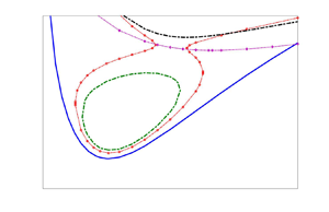
Figure 4. The neutral stability curves and variation of the critical Rayleigh number with the dimensionless strength of the HTG at  ${Bi=10^{-5} }$ and
  $Pr=7$. (a) Neutral stability curves for select values of
  $\eta$. An increasing
  $\eta$ decreases the neutral stability island size, which disappears at
  $\eta =0.21$. (b) Variation of
  $Ra_c$ with
  $\eta$. The long wave mode due to VTG forms an island of instability as a result of stabilisation by the imposed HTG. The island is constrained to
  $\eta <0.21$.
The disappearance of the island of instability in  $k$–
$k$– $Ra$ space at a sufficiently high
  $\eta$ leads to the formation of a corresponding island of instability in the
  $\eta$–
 $Ra_c$ parametric space as shown in figure 4(b). The base state is unstable inside the island and stable outside of the island. It must be noted that a similar island of instability was also predicted by Patne & Oron (Reference Patne and Oron2022) for a poorly conducting bottom wall. The physical mechanism by which such a stabilisation manifests has been discussed in § 6. The absence of instability outside of the island also implies for
  $\eta \rightarrow \infty$, i.e. purely HTG, the base flow will remain linearly stable.
The buoyancy instabilities are typically observed in thick fluid layers due to the strong influence of thermocapillary forces for thin layers. A ratio of the Rayleigh number to the Marangoni number, i.e.  $Ra/Ma \sim d^2$, provided that other parameters are constant. Thus, typically, it is assumed that the thermocapillary instabilities will be relevant for thin layers. From figure 4(b), the imposed HTG stabilises the VTG mode. However, from Patne et al. (Reference Patne, Agnon and Oron2021a), thermocapillary instabilities exist in the same setting since the imposed OTG leads to a new mode of instability. Thus, we conjecture that for water with
  $Pr=7$, one could experimentally observe a thermocapillary mode even for liquid layers with
  $d \sim O(10^{-2})$ m.
For liquid layers with  $d \gg O(10^{-2})$ m,
  $Bi \gg 0.1$. In this case, for sufficiently high
  $\eta$, from the base-state temperature profile (2.4c), the induced linear VTG term, namely
  $({-Bi \, \eta ^2 \, Ra}/{320 (1 + Bi)}) y$ becomes relevant. As mentioned in § 2, this term arises due to the imposed HTG, and it is linear in
  $y$, thus termed induced linear VTG. This term has the same sign as the imposed VTG and thus reinforces the imposed VTG. This reinforcement neutralises the stabilising effect of the induced quintic VTG term. This results in the existence of a new streamwise mode of instability shown in figure 5, which arises at a much higher
  $k$ and
  $\eta$ than the VTG mode. Additionally, the new mode is an upstream travelling mode since
  $s_i>0$ while the VTG mode is a downstream mode for non-zero
  $\eta$.

Figure 5. Variation of  $s_r$ in the
  $s_i\unicode{x2013}s_r$ plane at
  $Pr=7, k=6, \eta =10$ and
  $Bi=10$. The figure shows the existence of a new mode of instability at high
  $\eta$.
The origin of the new mode can be well understood using the neutral stability curves shown in figure 6(a). From the neutral stability curves for  $Pr=7$ and
  $Bi=10^{-5}$, from figure 4(a), an increasing
  $\eta$ leads to the formation of the island of instability in the
  $k\unicode{x2013}Ra$ plane. This island shrinks with increasing
  $\eta$ to disappear eventually. From figure 6(a), for
  $\eta \neq 0$, the neutral stability curve forms a pinch point at the higher
  $Ra$ part, as shown in the curve for
  $\eta =0.2$. An increasing
  $\eta$ then pinches the neutral stability curve and divides it into two separate neutral stability curves for the VTG and new modes (see the curves for
  $\eta =0.25$). The VTG mode also forms an island of instability much akin to the case of
  $Bi=10^{-5}$ and
  $Pr=7$ shown in figure 4(a). Upon further increase in
  $\eta$, the VTG mode vanishes while the neutral stability curve for the new mode shifts towards lower
  $Ra$, implying its destabilisation by an increasing
  $\eta$.

Figure 6. The neutral stability curves and variation of  $Ra_c$ with
  $\eta$ at
  $Bi=10$ and
  $Pr=7$. (a) Neutral stability curves for select values of
  $\eta$. The new mode originates as a high
  $Ra$ part of the neutral stability curve. For
  $\eta =0.6$, the VTG mode completely disappears while the new mode dominates the instability of the layer. Thus, the neutral stability curve for the VTG mode is absent. (b) Variation of
  $Ra_c$ with
  $\eta$. The new mode exhibits
  $Ra_c \sim 1/\eta$ scaling for
  $\eta >0.7$.
The island of instability in the  $\eta$–
 $Ra_c$ is absent for liquid layers with
  $Bi=10$ due to the presence of the new mode. Instead, from figure 6(b), the VTG mode passes the baton to the new mode with the latter exhibiting a much higher
  $Ra_c$ initially, which decreases with an increasing
  $\eta$.
If the induced linear VTG term were to only counter the stabilising influence of the induced quintic VTG term on the VTG mode, then for higher  $\eta$ as well,
  $Ra_c$ should achieve a constant value corresponding to a liquid layer subjected to a purely VTG. However, from figure 6(b), it is clear that such is not the case. Instead,
  $Ra_c$ decreases with an increasing
  $\eta$ exhibiting the scaling
  $Ra_c \sim 1/\eta$, implying that the induced linear VTG term not only counters the stabilising influence of the induced quintic VTG term but also leads to further destabilisation in conjunction with other effects. The physical mechanism responsible for the existence of the new mode is discussed in §§ 5 and 6. The contour plots of
  $v'_y$ for the new streamwise mode are shown in figure 7. The structure of the rolls readily indicates the convective nature of the new mode and upstream travelling direction. Additionally, these convection rolls show a strong resemblance with those predicted by Smith & Davis (Reference Smith and Davis1983a) for hydrothermal waves in a liquid layer subjected to a purely HTG.

Figure 7. The contour plots of  $v'_y$ for the new streamwise mode at
  $Ra=836.1, Bi=10, k=7, Pr=7$ and
  $\eta =10$ such that the new mode is marginally stable. The appearance of the streamwise convection rolls resembles the hydrothermal waves predicted by Smith & Davis (Reference Smith and Davis1983a).
The scaling  $Ra_c \sim 1/\eta$ also implies that for a purely HTG (
 $\eta \rightarrow \infty$),
  $Ra_c \rightarrow 0$. For example, for
  $\eta =10^5$, the stability analysis predicts
  $Ra_c \sim 0.07$. Thus, when the system is subjected to a purely HTG, the base flow will be purely destabilised by the imposed HTG, and the critical Rayleigh number for the instability can be estimated in terms of the horizontal Rayleigh number
  $Ra_H$ using relation
  $Ra_H = \eta Ra$.
4.1.2. For $Pr<1$

For  $Pr=7$ and
  $Bi \ll 1$, there was an absence of buoyancy instability for
  $\eta >0.21$ as shown in figure 4. This occurs due to the strong stabilising effect of the imposed HTG through the induced quintic VTG term of the base state temperature profile (2.4c). However, for a non-zero
  $Bi$, a new mode of instability arises as a result of the imposed VTG reinforcement by the induced VTG. We follow similar steps here by first analysing the case with
  $Bi \ll 1$ and then for non-zero
  $Bi$.
$Bi$.
For  $Bi\ll 1$ and
  $Pr=0.1$, from figure 8, similar to the case with
  $Pr=7$, an increasing
  $\eta$ has a strong stabilising effect on the VTG mode. However, for
  $\eta >0.15$, the HTG has a destabilising effect on the same mode. For
  $\eta > 0.6$, the curve shows the characteristic scaling
  $Ra_c \sim 1/\eta$. Thus, this leads to a rather unique-shaped curve in the
  $\eta$–
 $Ra_c$ parametric space. It must be noted that in the case of a poorly conducting bottom wall studied by Patne & Oron (Reference Patne and Oron2022), a similar behaviour was predicted in contrast to the perfectly conducting bottom wall considered here. This indicates that for low
  $Bi$ and
  $Pr=0.1$, the thermal conductivity of the bottom wall does not alter the stability picture. In this case, also, owing to the scaling
  $Ra_c \sim 1/\eta$,
  $Ra_c \rightarrow 0$ as
  $\eta \rightarrow \infty$ since for
  $\eta =10^5$,
  $Ra_c \sim 0.055$. Thus, the liquid layer will be unstable even if it is subjected to a purely HTG.

Figure 8. Neutral stability curves in the  $k\unicode{x2013}Ra$ plane (a) and variation of
  $Ra_c$ with
  $\eta$ (b) at
  $Pr=0.1$ and
  ${Bi=10^{-5}}$. Similar to the case with
  $Pr=7$, at low
  $\eta$, an increasing
  $\eta$ stabilises the VTG mode. However, for
  $\eta > 0.15$, the VTG mode is destabilised by an increasing
  $\eta$.
For  $Pr=0.01$ and vanishing
  $Bi$, the HTG fails to stabilise the VTG mode. Instead, the HTG enhances the VTG mode to result in a more destructive VTG mode by lowering
  $Ra_c$ as indicated by the shifting of the neutral stability curves to lower
  $Ra$ in figure 9(a). The variation of
  $Ra_c$ with
  $\eta$ is shown in figure 9(b), affirming the conclusions of the neutral stability curves. Similar to the case of
  $Pr=0.1$ shown in figure 8(b), for
  $\eta >0.15$, the
  $Ra_c$ curve exhibits the scaling
  $Ra_c \sim 1/\eta$. For a poorly conducting bottom wall, Patne & Oron (Reference Patne and Oron2022) predicted the presence of a new mode of instability at low
  $Pr$, which bifurcated from the island of instability at low
  $\eta$. In the present case, there is an absence of a new mode; instead, the VTG mode gets destabilised by imposed HTG, which leads to the predicted stability picture. From figure 8(b),
  $Ra_c \sim 1/\eta$, thus
  $Ra_c \rightarrow 0$ in the extreme limit
  $\eta \rightarrow \infty$. For example, for
  $\eta =10^5$,
  $Ra_c \sim 0.00085$. Thus, the liquid layer can become unstable even in the absence of the imposed VTG. As discussed in §§ 5 and 6, the HTG achieves destabilisation through the Reynolds stress work, which becomes a bridge in transferring the kinetic energy from the base flow to the perturbations.

Figure 9. Neutral stability curves (a) and  $Ra_c$ variation with
  $\eta$ (b) at
  ${Bi=10^{-5} }$ and
  $Pr=0.01$. The neutral stability curves appear similar to those for
  $Pr=0.1$ in figure 8(a). However, unlike the
  $Pr=0.1$ case, from (b), the VTG mode is destabilised by an increasing
  $\eta$ irrespective of the value of
  $\eta$.
For non-zero  $Bi$ and
  $Pr=0.01$, the variation of
  $Ra_c$ with
  $\eta$ is shown in figure 10. While a non-zero
  $Bi$ leads to a new streamwise mode for
  $Pr=7$, figure 10 shows that there is absence of such a mode for
  $Pr=0.01$. An increasing
  $Bi$ stabilises the VTG mode in the absence of the imposed HTG. However, from figures 9(b) and 10, the imposed HTG has a destabilising effect on the same VTG mode irrespective of the
  $Bi$ value for low
  $Pr$. This destabilisation by the HTG nullifies the stabilising effect of the increasing
  $Bi$ at sufficiently high
  $\eta$. Thus, as
  $Bi$ increases, the critical parameter curve shifts to higher
  $Ra_c$ for low and intermediate values of
  $\eta$, while in the region where
  $\eta$ is high, the HTG dominates and removes the effect of
  $Bi$. This leads to the merging of the curves for different
  $Bi$ at high
  $\eta$. Note that, as explained later in § 6, for low
  $Pr$ and high
  $\eta$, the Reynolds stress work dominates the other perturbation energy sources/sinks, which could also explain the irrelevance of
  $Bi$ at high
  $\eta$.

Figure 10. The variation of  $Ra_c$ with
  $\eta$ at
  $Pr=0.01$ for two value of
  $Bi$. At high
  $\eta$, the curves for different values of
  $Bi$ merge, showing the irrelevance of
  $Bi$ when HTG is stronger than the VTG.
4.2. Spanwise mode ($k=0$)

4.2.1. For $Pr>1$

For  $Pr=7$ and
  $Bi \ll 1$, the spanwise mode is also strongly stabilised by the imposed HTG owing to the induced quintic VTG term in the base state temperature profile (2.4c). From figure 2, the streamwise VTG mode becomes a downstream mode of instability (since
  $s_i<0$) due to the imposed HTG while the spanwise mode remains stationary (since
  $s_i=0$). Similar to the island of instability for the streamwise mode shown in figure 4, the spanwise mode also forms an island of instability in the
  $k\unicode{x2013}Ra$ plane, not shown here for brevity. From figure 11, the spanwise VTG mode also forms an island of instability in
  $\eta$–
 $Ra_c$ space.

Figure 11. The island of instability in  $\eta$–
 $Ra_c$ parametric space for the spanwise VTG mode at
  $Pr=7$ and
  ${Bi=10^{-5}}$. Similar to the streamwise VTG mode, the imposed HTG has a strong stabilising effect on the VTG mode.
As we change  $Bi$ from
  $0$ to
  $10$ while keeping
  $Pr=7$, similar to the streamwise mode, a new spanwise mode originates. The neutral stability curves for the same are shown in figure 12(a). At
  $\eta =0.213$, the neutral stability curve forms a pinch point at the higher
  $Ra$ part. This pinch further develops and divides the neutral stability curves into two separate curves for the VTG and new modes (see the curves for
  $\eta =0.25$). Upon further increase in
  $\eta$, the VTG mode vanishes while the neutral stability curve for the new mode shifts towards lower
  $Ra$, implying its destabilisation by an increasing
  $\eta$.

Figure 12. (a) The effect of variation in  $\eta$ on the neutral stability curves in the
  $m\unicode{x2013}Ra$ plane at
  $Pr=7$ and
  $Bi=10$. The figure demonstrates the origin of the new spanwise mode in the
  $m\unicode{x2013}Ra$ plane. (b) The variation of
  $Ra_c$ with
  $\eta$ for
  $Pr=7$. (c) The variation of the critical spanwise wavenumber
  $m_c$ with
  $\eta$ for
  $Pr=7$.
The variation of  $Ra_c$ due to variation in
  $\eta$ for
  $Bi=1,10$ and
  $Pr=7$ is shown in figure 12(b). An increasing
  $Bi$ has a stabilising effect on the VTG mode even in the absence of the imposed HTG. Additionally, the imposed HTG also has a stabilising influence on the VTG mode. This leads to the shifting of the curve in the
  $\eta \unicode{x2013}Ra_c$ plane to a higher
  $Ra_c$ value for
  $\eta <0.3$. However, an increasing
  $Bi$ has a destabilising effect on the new spanwise mode. Thus, for
  $\eta >0.3$, the curve shifts downward with increasing
  $\eta$. As explained in § 6, the lowering of
  $Ra_c$ due to increasing
  $Bi$ for the new mode is a direct result of the influence of the induced linear VTG term in the base state temperature (2.4c). Irrespective of the value of
  $Bi$, for
  $\eta >0.3$, the curves exhibit characteristic scaling
  $Ra_c \sim 1/\eta$. From figure 12(c), for
  $\eta <0.3$, where the VTG mode is the dominant mode,
  $m_c$ is almost constant. Corresponding to the jump in
  $Ra_c$ curves of figure 12(b), where the dominant mode switches from the VTG mode to the new spanwise mode curve, there is also a jump in
  $m_c$ curves. At high
  $\eta$,
  $m_c$ for the new spanwise mode also achieves a constant value with higher
  $Bi$ systems having lower
  $m_c$. The structure of the convection rolls due to the new spanwise mode is shown in figure 13. The form of the rolls is similar to that for the VTG mode except for a change in the velocity contour density near
  $y=0,1$. For the new spanwise mode, similar to the new streamwise mode, as
  $\eta \rightarrow \infty$,
  $Ra_c \rightarrow 0$ implies the existence of an unstable flow even in the limit of a purely imposed HTG.

Figure 13. The contour plots of  $v'_y$ for the new spanwise mode at
  $Ra=705.15, Bi=10, m=7, Pr=7$ and
  $\eta =10$ such that
  $s_r \sim 0$ for the new spanwise mode. The rolls exhibit a structure similar to the purely VTG rolls shown in figure 3 owing to the stationary nature of the new spanwise mode.
4.2.2. For $Pr<1$

For  $Pr=0.01$, unlike the streamwise VTG mode, the imposed HTG has a much more powerful impact, as shown in figure 14(a). For
  $\eta < 0.0188$, there is only one unstable mode. An increasing
  $\eta$ leads to an additional unstable mode. The original VTG mode and the new unstable mode have the same
  $s_i$ but different
  $s_r$. These modes at
  $\eta = 0.018862$ possess equal growth rates. Any further increase in
  $\eta$ leads to the origin of a pair of unstable modes having the same
  $s_r$ and
  $|s_i|$ but an opposite sign of
  $s_i$. Thus, these two modes travel in opposite directions. The imposed HTG initially stabilises the newly formed pair until
  $\eta =0.2$, beyond which the HTG destabilises. This initial stabilisation leads to a small hump in the curve, but at high
  $\eta$, the curve shows the scaling
  $Ra_c \sim 1/\eta$ as shown in as shown in figure 14(b). It must be noted that both the modes in the pair possess the same
  $Ra_c$.

Figure 14. (a) Movement of eigenvalues in the  $s_i\unicode{x2013}s_r$ plane at
  $Pr=0.01, m=2, Ra=900$ and
  ${Bi=10^{-5}}$. The figure demonstrates the existence of a pair of unstable spanwise modes for low
  $Pr$ originating from two unstable stationary spanwise modes. (b) The effect of variation in
  $\eta$ on
  $Ra_c$ at
  $Pr=0.01$ and
  ${Bi=10^{-5} }$ for the spanwise VTG mode. For
  $0.01 < \eta < 0.2$, the imposed HTG stabilises the VTG mode. For
  $\eta >0.2$, an increasing
  $\eta$ destabilises the VTG mode.
For  $Bi \neq 0$, it is similar to the streamwise mode as shown in figure 15. For
  $Pr=0.01$ and
  $Bi=1$, as
  $\eta \ll 1$, the critical wavenumber attains a constant value
  ${\sim }2.3$ while in the limit
  $\eta \gg 1$,
  $m_c \sim 1.35$. Similarly for
  $Bi=10$,
  $m_c$ in the limits
  $\eta \ll 1$ and
  $\eta \gg 1$ is
  $m_c \sim 2.6$ and
  $m_c \sim 1.75$, respectively.

Figure 15. The variation of  $Ra_c$ with
  $\eta$. An increasing
  $Bi$ number has a purely stabilising effect on the spanwise mode for low
  $Pr$.
$Pr$.
4.3. Oblique modes ($k \neq 0$ and $m \neq 0$)


In the previous two §§ 4.1 and 4.2, we have analysed the stability of the streamwise mode for which  $m=0$ and spanwise mode for which
  $k=0$. Along with these modes, there are also oblique modes possessing
  $k\neq 0$ and
  $m\neq 0$. This section aims to analyse these oblique modes. If there exists an oblique mode, which has
  $Ra_c$ lower than the streamwise mode for a particular combination of
  $k$ and
  $m$, then the growth rate
  $s_r$ must increase for a particular combination of
  $k$ and
  $m$. To demonstrate, here we consider two cases, one where the VTG mode determines the stability of the layer (figure 16a) and the other where the new mode controls the stability of the layer (figure 16b).

Figure 16. (a) The VTG mode exhibits a lower growth rate as it becomes an oblique mode due to an increasing spanwise wavenumber  $m$ at
  $\eta =10, Pr=0.01, {Bi=10^{-5}}, Ra=15$ and
  $k=1.5$. The parameter
  $m$ has been increased in steps of
  $0.25$, and the mode with the highest
  $s_r$ is for
  $m=0$. For
  $k=0$, the mode leads to a pair of spanwise modes, as shown in figure 14(a). (b) The new spanwise mode is stabilised due to increasing streamwise wavenumber
  $k$ for
  $\eta =10, Pr=7, Bi=10, Ra=750$ and
  $m=7$. The point with the highest
  $s_r$ corresponds to
  $k=0$, and
  $k$ has been increased in steps of unity. The same mode for
  $m=0$ becomes the new streamwise mode whose neutral stability curves and
  $Ra_c$ variation with
  $\eta$ are given in figure 6.
For the parameter set  $\eta =10, Pr=0.01, Bi=10^{-5}, Ra=15$, the streamwise VTG mode becomes unstable at a much lower
  $Ra$ than the spanwise VTG mode; thus, the former is the dominant mode. In this case, we probe for a more unstable oblique mode. Thus, the spanwise wavenumber (
 $m$) is increased while keeping other parameters constant in figure 16(a). This increase in
  $m$ implies we are looking at oblique modes. It turns out that the growth rate of the oblique modes is always lower than the streamwise mode. It must be noted that although not shown here, we have also explored different combinations of
  $k$ and
  $m$; still, the analysis did not predict the existence of a mode with higher
  $s_r$.
Figure 16(b) shows the second case where the new mode determines the stability of the layer. In this case, the new spanwise mode has a lower  $Ra_c$ than the new streamwise mode. Once again, we probe for an oblique mode with a higher
  $s_r$ than the spanwise mode by trying different combinations of
  $k$ and
  $m$. One such exercise is shown in figure 16(b) by keeping
  $m$ constant and varying
  $k$. An increasing
  $k$ leads to a decrease in
  $s_r$, thereby indicating that the new spanwise mode is more unstable. Thus, for the parameter range explored in the present study, either streamwise or spanwise mode is the most unstable or dominant mode of instability. The oblique modes will always have
  $s_r$ lying between these two modes. Thus, we will not be exploring these modes in detail.
4.4. Dominant mode
From §§ 4.1, 4.2 and 4.3, for a given parameter set, various modes of instability become unstable. Experimentally, as  $Ra$ is increased, the mode with the lowest
  $Ra_c$ or the dominant mode becomes unstable first, followed by the other modes. The dominant mode also exhibits a higher growth rate than the other modes; thus, the dominant mode is expected to be observed in the experiments. From § 4.3, the oblique modes always have a growth rate less than the streamwise or spanwise mode. Thus, in this section, we compare the streamwise and spanwise modes based on
  $Ra_c$ required to destabilise the mode and provide a guideline for the experiments to observe the instabilities predicted here.
4.4.1. For $Pr=7$

For  $Bi \ll 1$, from figures 4(b) and 11, both the streamwise and spanwise VTG modes form an island of instability in
  $\eta$–
 $Ra_c$ space. The comparison of these instability islands is shown in figure 17(a). The spanwise VTG mode becomes unstable at a lower
  $Ra_c$ than the streamwise VTG mode, implying that the former is the dominant mode in this case. Additionally, the island for the spanwise VTG mode extends to a larger
  $\eta$ than for the streamwise VTG mode, thereby showing that the former resists the stabilising influence of the induced quintic VTG term better than the latter.

Figure 17. A comparison of  $Ra_c$ for the streamwise and spanwise modes to determine the dominant mode of instability for
  ${Bi=10^{-5}}$ and
  $Bi=10$. (a) The
  $Ra_c$ required for the spanwise VTG mode is lesser than the streamwise VTG mode for
  $\eta >0.03$; thus, the former is the dominant mode of instability. (b) In this case also, the spanwise mode is the dominant mode.
For  $Bi=10$, new streamwise and spanwise modes exist, which determine the stability of the layer. The comparison of
  $Ra_c$ for the streamwise and spanwise new modes is shown in figure 17(b). Here, as well, the streamwise new mode has a higher
  $Ra_c$ than the spanwise new mode, indicating that the latter is the dominant mode of instability. To conclude, if one were to conduct experiments for the present system and the experimental fluid is water (
 $Pr \sim 7$), then the experimentally observed instability could be due to the spanwise mode irrespective of the
  $Bi$ value.
4.4.2. For $Pr=0.01$

From §§ 4.1 and 4.2, the induced quintic VTG term fails to stabilise the streamwise and spanwise VTG modes completely, unlike the  $Pr=7$ case. Also, even for non-zero
  $Bi$, there is an absence of a new mode of instability. A comparison of
  $Ra_c$ for the streamwise and spanwise modes for two values of
  $Bi$ is shown in figure 18. For
  $0.01<\eta < 0.2$, the imposed HTG has a stabilising effect on the spanwise mode, which leads to an increase in
  $Ra_c$, but this stabilisation disappears for
  $\eta >0.2$. This stabilisation separates the behaviour of the streamwise mode since an increasing
  $\eta$ has a monotonic destabilising effect on the streamwise mode. This difference established at low
  $\eta$ becomes crucial at high
  $\eta$ as well by making the streamwise mode a dominant mode of instability for
  $Pr=0.01$. The scenario remains unchanged even as
  $Bi$ increases to
  $10$, as shown in figure 18(b).

Figure 18. The  $Ra_c$ required for the spanwise mode is higher than the streamwise mode for
  $\eta >0.01$; thus, the latter is the dominant mode of instability irrespective of the
  $Bi$ value for
  $Pr=0.01$. Here (a)
  $Bi=10^{-5}$; (b)
  $Bi=10$.
5. Perturbation energy budget analysis
In § 4, the stability analysis predicted new streamwise and spanwise modes for  $Bi \neq 0$ and
  $Pr=7$. To understand the factors responsible for the existence of these modes, here we analyse the perturbation energy budget using the approach of Hu, He & Chen (Reference Hu, He and Chen2016), Hu et al. (Reference Hu, He, Chen and Liu2017), Patne et al. (Reference Patne, Agnon and Oron2021a) and Patne & Oron (Reference Patne and Oron2022). To accomplish this, the momentum conservation equations (2.2b) are linearised around an arbitrary base state to yield
 \begin{equation} \frac{1}{Pr} \frac{\partial \boldsymbol{v}^\prime}{\partial t} ={-}\boldsymbol{\nabla} p^\prime + \boldsymbol{\nabla} \boldsymbol{\cdot} \boldsymbol{\tau}^\prime + Ra T' \boldsymbol{\nabla} y - \frac{1}{Pr} \left[ (\boldsymbol{v'} \boldsymbol{\cdot}\boldsymbol{\nabla}) \boldsymbol{\bar{v}} + (\boldsymbol{\bar{v}} \boldsymbol{\cdot}\boldsymbol{\nabla}) \boldsymbol{v'} \right], \end{equation}
where  $\boldsymbol {\tau }$ is the stress tensor and a prime,
  $'$, implies a perturbation quantity. To obtain the perturbation energy equation, (5.1) is scalar multiplied by the perturbation velocity vector
  ${\boldsymbol {v}}^\prime$. The resulting equation is then integrated over the liquid layer to yield
 \begin{align} \frac{1}{Pr} \frac{\partial E}{\partial t} &={-} \frac{1}{2} \int \boldsymbol{\tau}^\prime : \boldsymbol{\dot{\gamma}^\prime} \, {\rm d}V + Ra \int T' \, v'_y \, {\rm d}V - \frac{1}{Pr} \int \boldsymbol{v'} \boldsymbol{\cdot} \boldsymbol{\bar{\dot{\gamma}} } \boldsymbol{\cdot} \boldsymbol{v'} \, {\rm d}V \nonumber\\ &\equiv{-} I_b + I_{RB} - I_R, \end{align}
 \begin{equation} E= \tfrac{1}{2}\int{\boldsymbol{v}}^\prime \boldsymbol{\cdot}{\boldsymbol{v}}^\prime\,{\rm d}V. \end{equation}
Here, the integrals  $I_b, I_{RB}$ and
  $I_{R}$ are the bulk stress work, Rayleigh–Bénard integral or buoyancy work, and the Reynolds stress work (Drazin Reference Drazin2002), respectively, and
  ${\rm d}V$ is the volume element. The quantities
  $\boldsymbol {\dot {\gamma }} ^\prime = \boldsymbol {\nabla } \boldsymbol {v}^\prime + \boldsymbol {\nabla } {\boldsymbol {v}^\prime }^T$ and
  $\boldsymbol {\bar {\dot {\gamma }} }= \boldsymbol {\nabla } \boldsymbol {\bar {v}} + \boldsymbol {\nabla } \boldsymbol {\bar {v}}^T$ are the strain-rate tensors in the perturbed and base states, respectively. It must be noted that while obtaining the above equation, we have used the continuity equation,
  $\boldsymbol {\nabla }\boldsymbol {\cdot }\boldsymbol {v'}=0$. The pressure perturbation energy term vanishes at the bottom wall and free surface due to the vanishing normal velocity perturbations.
The bulk stress work  $I_b = \frac {1}{2} \int \boldsymbol {\tau }^\prime : \boldsymbol {\dot {\gamma }^\prime } \, {\rm d}V$ represents viscous dissipation of the perturbation energy. For a Newtonian fluid,
  $\tau '_{ij} = \gamma '_{ij}$, thus,
  $I_b = \frac {1}{2} \boldsymbol {\tau }^\prime : \boldsymbol {\dot {\gamma }}^\prime = \frac {1}{2} \gamma '_{ij}\gamma '_{ji} \geqslant 0$. This leads to the immediate conclusion that the bulk stress work will always lead to a decrease in the perturbation energy for a Newtonian fluid. The same is not the case for viscoelastic fluids as predicted by Hu et al. (Reference Hu, He and Chen2016, Reference Hu, He, Chen and Liu2017) and Patne et al. (Reference Patne, Agnon and Oron2021a, Reference Patne, Agnon and Oron2020a) where
  $I_b$ could lead to new instabilities.
The Rayleigh–Bénard integral or buoyancy work  $I_{RB}$ arises purely due to the buoyancy. Typically, for a liquid layer subjected to a purely negative VTG, causing unstable density stratification,
  $I_{RB}$ is positive, thereby leading to the VTG mode. To accomplish that,
  $I_{RB}$ must overcome the stabilising impact of the dissipation factors, such as viscous forces and thermal diffusion of the energy.
The third integral, viz., the Reynolds stress work ( $I_{R}$), arises purely as a consequence of the imposed HTG. For a liquid layer subjected to a purely VTG, the base state is a vanishing velocity field. In that case
  $I_{R}=({1}/{Pr} )\int \boldsymbol {v'} \boldsymbol {\cdot } \boldsymbol {\bar {\dot {\gamma }} } \boldsymbol {\cdot } \boldsymbol {v'} \, {\rm d}V$ will vanish since
  $\boldsymbol {\bar {\dot {\gamma }} } = 0$. Thus, it does not contribute to the VTG mode. However, in the present case, due to the HTG component of the imposed OTG, the base state velocity in the
  $x$ direction is non-zero, thus
  $\boldsymbol {\bar {\dot {\gamma }} } \neq 0$. The integral
  $I_{R}$ represents a volume-averaged correlation between the perturbations in the horizontal and vertical components of the velocity field. This integral is also responsible for the energy exchange between the base state and the perturbation fields. The presence of
  ${1}/{Pr}$ in the integral
  $I_{R}$ indicates that for low
  $Pr$, this term will play a major role in determining the stability of the layer, which is indeed the case as discussed below. Furthermore, the base state strain-rate tensor
  $\boldsymbol {\bar {\dot {\gamma }} }$ directly depends on
  $\eta$. Thus, an increasing
  $\eta$ will lead to an increase in
  $\boldsymbol {\bar {\dot {\gamma }} }$ thereby enhancing the importance of the Reynolds stress work in influencing the stability of the layer.
Before proceeding with the numerical calculations of the integrals, the following conclusions can be drawn by using the definitions of the integrals. The absolute values of the integrals may not provide the exact roles of the different terms. Thus, we normalise the integrals by the absolute value of  $I_{RB}$. From (5.2), we have
 \begin{equation} \frac{I_b}{I_{RB}} = \frac{1}{2Ra} \frac{ \displaystyle\int \boldsymbol{\tau}^\prime : \boldsymbol{\dot{\gamma}^\prime } \, {\rm d}V}{ \displaystyle\int T' \, v'_y \, {\rm d}V}. \end{equation}
As explained later in § 6, for the buoyancy convection to exist, the destabilising forces, i.e. Raleigh–Bénard work term, must overcome the viscous dissipation forces represented by  $I_b$. From above expression, as
  $Ra \rightarrow \infty$,
  ${I_b}/{I_{RB}} \rightarrow 0$. Physically, this implies that as
  $Ra$ increases, the Rayleigh–Bénard work term overpowers the viscous dissipation term to result in an instability, which is indeed the case for
  $\eta =0$.
The other ratio is
 \begin{equation} \frac{I_R}{I_{RB}} = \frac{1}{Pr \, Ra} \frac{ \displaystyle\int \boldsymbol{v'} \boldsymbol{\cdot} \boldsymbol{\bar{\dot{\gamma}} } \boldsymbol{\cdot} \boldsymbol{v'} \, {\rm d}V}{ \displaystyle\int T' \, v'_y \, {\rm d}V}. \end{equation}
Only  $\bar {\dot {\gamma }}_{xy}$ and
  $\bar {\dot {\gamma }}_{yx}$ components of the base state strain-rate are non-zero. Thus, the above equation using the base state velocity (2.4a) modifies to
 \begin{equation} \frac{I_R}{I_{RB}} ={-}\frac{\eta}{4 Pr} \frac{ \displaystyle\int (y-1) (4y-1) v'_x v'_y \, {\rm d}V}{ \displaystyle\int T' \, v'_y \, {\rm d}V}. \end{equation}
This implies that an increase in  $Ra$ will not directly affect the value of this ratio. Instead, it is the strength of the imposed HTG
  $\eta$ that will directly affect this ratio. Additionally, the presence of
  $Pr$ in the denominator implies that cases with the
  $Pr<1$ will have a better chance of being destabilised by the Reynolds stress work
  $I_R$. This is indeed the case from figures 8 and 9 where
  $Pr<1$ leads to the destabilisation of the VTG mode unlike in the case of
  $Pr=7$. The volume-averaged correlation
  $\int (y-1) (4y-1) v'_x v'_y \, {\rm d}V$ must be positive to contribute to the growth of the perturbations via (5.2).
We focus on the new streamwise mode and try to understand the impact of various terms in (5.2) in introducing the new modes. The values of the integrals normalised by the Rayleigh–Bénard integral for a set of parameters corresponding to the new streamwise mode in an unstable regime are given in table 1. The bulk stress work ( $I_b$) is positive and thus will lead to the dissipation of the perturbation energy. The Reynolds stress work (
 $I_R$), on the other hand, is always negative, implying that it will lead to the enhancement of the perturbation energy. For
  $\eta =1$, both normalised
  $I_b$ and
  $I_R$ are less than unity; thus, the Rayleigh–Bénard work term (
 $I_{RB}$) is larger than both the terms, indicating the major role of
  $I_{RB}$ in introducing the new mode of instability. It must be noted that the integral
  $I_{RB}$ could achieve such a high value as a direct result of the presence of the induced linear VTG term. This term, as noted in § 4, counters the stabilising influence of the induced quintic VTG term even for
  $\eta <1$ (see figure 6). The base-state velocity (2.4a) is proportional to
  $\eta$; thus, at low
  $\eta$, the integral
  $I_R$ would have a lower contribution. As
  $\eta$ increases, the value of
  $I_R$ also increases, and for
  $\eta =100$, it is two times larger than
  $I_{RB}$. Thus, while
  $I_{RB}$ plays a vital role in introducing the new mode,
  $I_R$ is the one which drives the new mode at high
  $\eta$.
Table 1. Values of the bulk stress work ( $I_b$) and Reynolds stress work (
 $I_R$) normalised by the buoyancy work (
 $I_{RB}$) in the energy balance equation (5.2) for the streamwise new mode at
  $Bi=10, k=7, m=0$ and
  $Pr=7$. In each case, the streamwise new mode is unstable. As expected, the normalised bulk stress work is positive, implying its stabilising influence. The normalised Reynolds work term is negative, thereby having a destabilising influence. The Rayleigh–Bénard work term is found to be positive for the above combination of parameters.

It must be noted that the perturbation energy analysis carried out here can only provide qualitative information about perturbation energy sources/sinks that may lead to destabilisation (Drazin Reference Drazin2002). However, the correct critical parameter values may be obtained only using the general linear stability analysis discussed in § 4.
6. Physical mechanism
From figure 4, the VTG mode is completely stabilised by the imposed HTG for vanishing  $Bi$ and
  $Pr>1$. While for
  $Pr<1$ and
  $Bi \sim 0$, the imposed HTG may have a stabilising effect at the beginning, but eventually, it leads to destabilisation of the VTG mode (see figures 8 and 9). For
  $Bi \neq 0$, new streamwise and spanwise modes appear as shown in figures 6 and 12. These modes do not exist when a liquid layer is subjected to a purely VTG but arise due to an interaction between the imposed VTG and HTG. This physical manifestation of the stabilising/destabilising effect of the imposed HTG remains to be understood, which is precisely the aim of this section.
A liquid layer subjected to a purely negative VTG (i.e. the bottom wall is at a higher temperature than the ambient gas) exhibits Rayleigh–Bénard convection due to the lighter liquid at the bottom and heavy liquid at the top owing to the temperature dependence of the liquid density. One can describe this convection phenomenon in terms of liquid movement as follows. Consider a liquid parcel located at  $y=y_0$. Assuming the density of the liquid is a linearly decreasing function of the temperature, the parcel located at a higher level
  $y=y_0+\Delta y$ will have a higher density than that of the liquid layer present at
  $y=y_0$. Here
  $\varDelta \ll 1$ and a positive quantity. Due to the imposed gravity field, the liquid parcel at
  $y=y_0$ will try to move to
  $y=y_0+\Delta y$. The viscous forces and thermal diffusion of the energy from the parcel to the surrounding liquid will oppose this movement. If the imposed VTG strength is strong enough, the parcel will overcome the viscous and thermal energy diffusion resistance and move to
  $y=y_0+\Delta y$, resulting in the buoyancy convection. For the convenience of discussion, this section will be divided into two subsections: (i)
  $Bi \ll 1$ and (ii)
  $Bi \neq 0$.
6.1. For $Bi \ll 1$

6.1.1. For $Pr>1$

From figure 4, the VTG mode is stabilised for  $\eta > 0.22$. Patne & Oron (Reference Patne and Oron2022) discussed the stabilisation of the longwave mode that originates due to the imposed VTG. Their analysis indicates the presence of an opposing VTG induced by the imposed HTG, which leads to the predicted stabilisation. From base state temperature (2.4c), at
  $Bi \rightarrow 0$, there is a linear term in
  $y$ with coefficient (
 $-1$) and a quintic polynomial term, viz., induced quintic VTG term. The average total VTG can then be obtained by differentiating base state temperature (2.4c) with respect to
  $y$ and integrating it over the fluid domain in the
  $y$ direction to obtain
 \begin{equation} \left(\frac{\partial {\bar{T}} }{\partial y} \right)_{avg} = \frac{\eta^2 Ra}{320}-1, \end{equation}
where the subscript  $avg$ indicates the average temperature gradient. The positive term
  ${\eta ^2 Ra}/{320}$ opposes the imposed VTG, thereby weakening it.
The physical manifestation of this stabilisation can be understood as follows. As discussed above, for the buoyancy instability to exist, the imposed VTG must be strong enough to overcome the resistance offered by the viscous forces and thermal diffusion away from the fluid parcel. The quintic polynomial term induced by the HTG weakens the imposed VTG, thus adding more resistance to the development of buoyancy instability. The weakened VTG fails to cause instability, thus the predicted stabilisation. At a sufficiently high  $\eta$, the average temperature gradient will become positive, thereby removing the possibility of the existence of buoyancy instability.
6.1.2. For $Pr<1$

As discussed in § 4, for  $Pr=0.1$ and
  $Pr=0.01$ (see figures 8 and 18), the imposed HTG fails to stabilise the VTG mode even for
  $Bi \ll 1$. The failure to stabilise the VTG mode could be understood from the perturbation energy analysis discussed in § 5 as follows.
For  $Bi \ll 1$, the induced linear VTG term does not affect the stability of the layer. Thus, the Rayleigh–Bénard work term
  $I_{RB}$ of (5.2), which plays a major role in introducing the new mode for
  $Bi \neq 0$, will not be of much relevance. Furthermore, the same
  $I_{RB}$ term fails to counter the stabilising effect of the imposed HTG through the induced quintic VTG term for
  $Pr=7$; thus, it is expected that such a term will not be the stability-determining term. In fact, at a sufficiently high
  $\eta$ from (6.1), owing to the induced quintic VTG term, the VTG will reverse the sign, resulting in a stable density stratification. In that case, the
  $I_{RB}$ term will have a stabilising effect. The bulk stress work term
  $I_b$ always leads to the viscous dissipation of the perturbation energy. The only remaining term that can lead to the growth of the perturbation energy is the Reynolds work term
  $I_R$. This term must overcome the stabilising effect of
  $I_b$ and
  $I_{RB}$ to result in instability. From figures 8 and 18, the
  $I_{R}$ term succeeds in this endeavour, thereby leading to the predicted results.
From perturbation energy equation (5.2),  $I_R$ has a multiplier
  $1/Pr$. Thus, as
  $Pr$ decreases, there will be a corresponding increase in the
  $I_R$ value. The base state velocity (2.4a) also has a multiplier
  $\eta Ra$. Thus, an increasing
  $\eta$ and
  $Ra$ and a decreasing
  $Pr$ will exacerbate the destabilisation caused by
  $I_R$, which succeeds for
  $Pr=0.01$. For
  $Pr=0.1$, from figure 8, due to a moderate value of
  $Pr$, the
  $I_{R}$ term is weak at low
  $\eta$; thus, the VTG mode is stabilised. However, as
  $\eta$ and
  $Ra$ increase, the
  $I_{R}$ term gains enough strength to counter the stabilising influence of
  $I_b$ and
  $I_{RB}$ resulting in the predicted curve.
6.2. For $Bi \neq 0$

From figures 6 and 12, for  $Bi \neq 0$, new streamwise and spanwise modes emerge. As noted in § 4, these modes originate due to the presence of the induced linear VTG term in the base-state temperature (2.4c), namely
  $({-Bi \, \eta ^2 \, Ra}/{320 (1 + Bi)} )y$. The physical mechanism by which the induced linear VTG term achieves this can be explained as follows.
The average total base state VTG for  $Bi \neq 0$ is
 \begin{equation} \left(\frac{\partial {\bar{T}} }{\partial y} \right)_{avg} = \frac{\eta^2 Ra}{320} - \frac{\eta^2 \, Bi \, Ra}{320(1+Bi)}-1. \end{equation}
For low  $Bi$, the term
  ${\eta ^2 \, Bi \, Ra}/{320(1+Bi)}$ will not be significant. However, as
  $Bi \rightarrow \infty$, the same term modifies to
  ${\eta ^2 Ra}/{320}$ which is exactly equal to the stabilising term. Thus, the induced linear VTG term can counter the effect of the induced quintic VTG term, provided that
  $Bi$ is sufficiently high. Once this induced quintic VTG term effect nullification occurs, the imposed VTG introduces the unstable density stratification, leading to the convection. At face value, we are returning to the liquid layer system subjected to a purely negative VTG. It turns out that the liquid layer is hiding a much more interesting dynamics, as described below.
To extract the additional information, we plot the variation of the base state temperature gradient obtained by differentiating (2.4c) with respect to  $y$. The result of such an exercise is shown in figure 19 in the parametric regime where the new streamwise mode is unstable. Unlike in the case of a liquid layer subjected to a purely VTG, where
  ${\partial \bar {T}}/{\partial y} <0$ throughout the liquid layer, there are two regions with
  ${\partial \bar {T}}/{\partial y} <0$. Thus, there are two regions which could potentially lead to the existence of the new mode. This raises the question, which of these two regions is responsible for the existence of the predicted new streamwise mode?

Figure 19. The base state temperature gradient variation with  $y$ at
  $Bi=10, \eta =10$ and
  $Ra=900$ where the streamwise new mode of instability is unstable. There are two regions with
  ${{\rm d}\bar {T}}/{{\rm d}y} <0$, i.e. with unstable density stratification.
The analysis of Patne & Oron (Reference Patne and Oron2022) for a similar problem with a poorly conducting bottom wall predicted a new mode of instability at low  $Pr$. Their analysis shows that the reverse flow shown in the schematic 1, near the bottom wall, could be responsible for the predicted new mode. In the present case, there is also the presence of reverse flow, which plays a role in causing an unstable stratification near the bottom wall shown in figure 19. However, as pointed out previously, the term
  $({-Bi \, \eta ^2 \, Ra}/{320 (1 + Bi)}) y$ could be responsible for the existence of the new mode of instability. This term contains the Biot number
  $Bi$, which enters through the thermal boundary condition at the free surface at
  $y=1$, and the second region with unstable stratification exists near the free surface. These arguments indicate that the unstably stratified region near the free surface is responsible for the existence of the new mode.
The requirement of sufficiently high  $Bi={q d}/{k_{th}}$ for the existence of the new mode also indicates that there is a need for efficient heat transfer from the liquid layer to the ambient gas, which then will result in the formation of a strong negative temperature gradient. As
  $Bi$ increases, the corresponding negative temperature gradient will also become severe, thereby exacerbating the instability and lowering
  $Ra_c$. This does not imply that
  $Bi \rightarrow \infty$ will lead to
  $Ra_c \rightarrow 0$ for sufficiently high
  $\eta$. For
  $Bi \gg 1$, it can be eliminated from the term
  ${-Bi \, \eta ^2 \, Ra}/{320 (1 + Bi)}$ by taking the limit
  $Bi \rightarrow \infty$ to obtain
  ${\eta ^2 Ra}/{320}$ thereby achieving a finite value. Thus, as
  $Bi$ increases beyond
  $10$, it will not lead to a much change in
  $Ra_c$ at high
  $\eta$. From perturbation energy budget analysis in § 5, an increasing
  $\eta$ also enhances the role of the Reynolds stress term, which dominates at high
  $\eta$ and the induced linear VTG term plays a supporting role.
7. Summary
In the present study, we carry out the linear stability analysis of a liquid layer supported by a perfectly conducting bottom wall and the other non-deformable free surface exposed to an inert ambient gas. The bottom wall, liquid layer and ambient gas are subjected to an OTG. The liquid density is assumed to be a linearly decreasing function of temperature. The imposed OTG consists of a negative VTG component, which leads to the canonical Rayleigh–Bénard convection and a HTG component, which leads to Hadley circulation. Using normal mode analysis, the linearised perturbation equations are reduced to a set of ordinary differential equations, becoming an eigenvalue problem in terms of growth rate  $s$. We employ the pseudospectral method (using Chebyshev polynomials) to solve the resulting eigenvalue problem. The numerical predictions are further explained using the perturbation energy budget analysis and physical arguments.
In the absence of the imposed HTG (i.e.  $\eta =0$), instability modes exist due to the imposed VTG. All the VTG modes of instability, viz., the streamwise (
 $k \neq 0$ and
  $m=0$), spanwise (
 $k=0$ and
  $m \neq 0$) and oblique modes (
 $k \neq 0$ and
  $m \neq 0$) become unstable at the same value of Rayleigh number
  $Ra =669$, thus the critical Rayleigh number
  $Ra_c =669$. Upon switching on the HTG, it leads to an induced linear VTG term (
 $({-Bi \, \eta ^2 \, Ra}/{320 (1 + Bi)}) y$) and an induced quintic VTG term (
 $({\eta ^2 \, Ra \, y^3 }/{960}) (20 -25y + 8 y^2)$).
For low  $Bi$, the induced linear VTG term can be neglected. For
  $Pr>1$, the induced quintic VTG term has a strong stabilising effect on the VTG modes. This stabilisation leads to an island of instability in the
  $k\unicode{x2013}Ra$ and
  $\eta \unicode{x2013}Ra_c$ planes for
  $Pr>1$. The physical arguments reveal that the induced quintic VTG term weakens the imposed VTG, which fails to overcome the resistance offered by the viscous dissipation and thermal energy diffusion, thereby increasing
  $Ra_c$. The spanwise VTG mode exhibits a larger island of instability than the streamwise VTG mode. Thus, the spanwise mode is the dominant mode of instability for
  $Pr>1$ and low
  $Bi$.
$Bi$.
For  $Pr=0.1$ and
  $Bi \ll 1$, the HTG stabilises the VTG mode for
  $\eta <0.15$ and the opposite effect for
  $\eta > 0.15$. In this case, the stabilisation occurs through the induced quintic VTG term. However, as
  $\eta$ increases beyond
  $0.15$, the Reynolds stress term, which facilitates the energy transfer from the base flow to the perturbations, becomes relevant. This term then leads to the subsequent destabilisation. At sufficiently high
  $\eta$, the
  $Ra_c$ versus
  $\eta$ curve exhibits
  $Ra_c \sim 1/\eta$ scaling. For
  $Pr=0.01$ and
  $Bi \ll 1$, the HTG has a destabilising effect for an arbitrary value of
  $\eta$ on the streamwise VTG mode. For the spanwise VTG mode, the HTG exhibits a destabilising effect except for low
  $\eta$. For
  $Pr=0.01$ and
  $Bi \ll 1$, the streamwise mode is the dominant mode of instability.
For  $Bi \neq 0$ and
  $Pr>1$, the induced linear VTG term becomes important. The perturbation energy analysis reveals that the same term reinforces the imposed VTG and helps cancel the stabilising effect of the induced quintic VTG term. This leads to the existence of new modes of instability. These new modes originate from the high
  $Ra$ part of the neutral stability curves for the VTG mode as
  $\eta$ increases. Thus, the liquid layer will exhibit instability at an arbitrary
  $\eta$ in contrast with the case for low
  $Bi$. The variation of the base state temperature gradient with
  $y$ reveals the existence of two zones with unstable density stratification, the first near the bottom wall and the second near the free surface. The presence of the Biot number (
 $Bi$) in the induced linear VTG term indicates that the unstable zone near the free surface could be the main culprit behind the existence of the new modes.
For  $Pr=7$, the new spanwise mode becomes more unstable at a lower
  $Ra$ than the new streamwise mode; thus, the spanwise mode is the dominant mode of instability. At
  $Pr=0.01$, an increasing
  $Bi$ stabilises the streamwise mode at low
  $\eta$ while at high
  $\eta$, curves in the
  $\eta \unicode{x2013}Ra_c$ plane for various
  $Bi$ merge. However, the spanwise mode at
  $Pr=0.01$ is stabilised by the increasing
  $Bi$ for the whole range of
  $\eta$. Thus, the streamwise mode is the dominant mode of instability for
  $Pr<1$, irrespective of the value of
  $Bi$.
$Bi$.
New streamwise and spanwise modes for  $Pr>1$ and finite
  $Bi$, and VTG mode for
  $Pr<1$ exhibit the scaling
  $Ra_c \sim 1/\eta$ in the limit of large
  $\eta$. Thus,
  $Ra_c \rightarrow 0$ as
  $\eta \rightarrow \infty$ for the above-mentioned modes. This implies the existence of an unstable base flow even if the imposed VTG is negligible. The results predicted here could be readily recast in terms of the Rayleigh number based on the imposed HTG,
  $Ra_H$. By definition, the Rayleigh number based on the imposed VTG and
  $Ra_H$ are related by
  $Ra_H = \eta Ra$.
The present analysis thus shows the possibility of using an OTG to intensify the mixing by manipulating buoyancy instabilities. Industrial applications could involve non-Newtonian fluids; thus, the present study could be extended to non-Newtonian fluids. Also, the instabilities predicted in the present study could be experimentally confirmed.
Funding
Authors acknowledge financial support from the Indian Institute of Technology Hyderabad, India, under grant SG/IITH/F280/2022-23/SG-118 and SERB-DST under grant SRG/2023/000223.
Declaration of interests
The authors report no conflict of interest.


