


1. Introduction
Experimental work on horizontal convection (HC) has attracted little attention compared with Rayleigh–Bénard convection. Despite the analysis of Jeffreys (Reference Jeffreys1925), who showed from fundamental thermodynamics that a differential buoyancy gradient along a constant geopotential height requires a residual circulation, the conclusion of Sandström (Reference Sandström1908), that only a very shallow surface circulation detached from a stratified interior at rest exists at high Rayleigh number, dominated the thinking on the subject for a long time (Sverdrup, Johnson & Fleming Reference Sverdrup, Johnson and Fleming1942; Defant Reference Defant1961). This position was later challenged by Rossby (Reference Rossby1965) based on laboratory experiments. Rossby showed that HC may indeed lead to a non-negligible overturning flow with a scaling analysis, which provided the first insights that, despite the small convective intensity of HC when compared with the Rayleigh–Bénard problem, HC could still produce a substantial residual circulation and be relevant for real-world applications.
A key difficulty in designing laboratory experiments in HC using heat as a stratifying agent is the need to prevent buoyancy gain or losses along surfaces other than the horizontal surface where forcing is applied. Wang & Huang (Reference Wang and Huang2005) used a nearly complete vacuum in a rectangular container to ensure an insulating boundary, while large Styrofoam slabs were used in the experiment of Mullarney, Griffiths & Hughes (Reference Mullarney, Griffiths and Hughes2004). Both sets of authors identified a regime transition at  ${Ra}\approx 10^{10}$ for differential heating in water. Each experiment provided similar scaling laws. However, an important difference could be found between the two experiments: the plume observed in the experiment of Wang & Huang (Reference Wang and Huang2005) did not fully reach the bottom, whereas the other experiment showed the contrary. Although this may be attributed to the insulating boundary, Gayen, Griffiths & Hughes (Reference Gayen, Griffiths and Hughes2014) performed direct numerical simulations of the set-up of Mullarney et al. and recovered a flow very similar to what was observed in the experiment. Therefore, these experiments raised the question of the role of the aspect ratio of the cavity in the flow. Working with differential heating is very attractive at first, as the viscosity of water can be increased (hence the Prandtl number) by using, for instance, glycerol. However, this method simultaneously decreases the Rayleigh number as in Rossby's original experiments, which prevented these experiments from reaching high Rayleigh numbers.
The large-Prandtl- and large-Rayleigh-number regimes have several important applications, ranging from mantle convection to industrial applications such as glass furnaces (Gramberg, Howell & Ockendon Reference Gramberg, Howell and Ockendon2007; Chiu-Webster, Hinch & Lister Reference Chiu-Webster, Hinch and Lister2008). Such regimes were theorized by Gramberg et al. (Reference Gramberg, Howell and Ockendon2007), who assumed that the return flow is distributed over the depth of the shallow layer, which makes the thin light layer move with a uniform velocity to the leading order. However, these findings were later questioned by Chiu-Webster et al. (Reference Chiu-Webster, Hinch and Lister2008), who showed that a laminar regime exists where only the densest fluid in the stratified boundary layer penetrates the entire depth of the box, the remainder returning at a shallow depth in a horizontal intrusion immediately adjacent to the boundary layer. In this case, diffusion between the interior and the relatively weak full-depth plume is crucial for both removing the density anomaly in the plume fluid and maintaining a stratification in the box interior. More recently, Ramme & Hansen (Reference Ramme and Hansen2019) investigated a similar regime but for higher Rayleigh numbers using two-dimensional numerical simulations. They report a transition to a steeper scaling than previously reported in Chiu-Webster et al. (Reference Chiu-Webster, Hinch and Lister2008). They report that the distribution of the forcing has only a small impact on the dynamics and, similarly, on the effect of shear-free or no-slip boundary conditions. They also noticed that the onset of instability introduces a steeper scaling for the Nusselt and Péclet numbers at Rayleigh numbers between  $10^8$ and
  $10^9$, which they conjectured to be associated with the transition observed in Shishkina & Wagner (Reference Shishkina and Wagner2016). However, it should be recalled that the transition observed in Shishkina & Wagner (Reference Shishkina and Wagner2016) was not induced by the onset of instabilities. It should also be noted that local steeper scaling than Rossby's 1/5, as, for instance, reported by Gayen et al. (Reference Gayen, Griffiths and Hughes2014), is associated with stability transitions. In addition, the effect of the aspect ratio remains to be examined at large Prandtl numbers, since in the Shishkina & Wagner (Reference Shishkina and Wagner2016) theory, the circulation has to span the entire depth of the domain, hence requiring, for instance, domains with large aspect ratios.
Griffiths & Gayen (Reference Griffiths and Gayen2015) considered the problem of HC forced by spatially periodic forcing. Their results showed that, for high Rayleigh numbers and small aspect ratios, the core would indeed fill with dense fluid and maintain a stratified interior. Their forcing, localized on a length scale smaller than the depth of the domain, and with variation in both horizontal directions, shows turbulence throughout the domain. Associated experiments were performed by Rosevear, Gayen & Griffiths (Reference Rosevear, Gayen and Griffiths2017), where they observed that the Nusselt number (a non-dimensional measure of the buoyancy flux) had a steeper scaling with respect to the Rayleigh number than the (laminar) Rossby scaling or the entrainment regime (Hughes & Griffiths Reference Hughes and Griffiths2008) and the intrusion regime (Chiu-Webster et al. Reference Chiu-Webster, Hinch and Lister2008). Here, we revisit their experiments, replacing porous brass plates with permeable membranes (Krishnamurti Reference Krishnamurti2003), which allows accurate measurements of the Nusselt number, as previously suggested in the experiment of Mullarney et al. (Reference Mullarney, Griffiths and Hughes2004). We further improve the method by providing evidence that steady states are reached for each experiment.
More recently, Matusik & Llewellyn-Smith (Reference Matusik and Llewellyn-Smith2019) analysed the response of surface buoyancy flux-driven convection to localized mechanical forcing where salt- and fresh-water fluxes were directed directly into the tank with pumps, while excess water was allowed to exit as an overflow. This set-up has the advantage of driving a localized surface forcing but cannot be considered as a closed system solely driven by buoyancy. The Whitehead & Wang (Reference Whitehead and Wang2008) and Stewart, Hughes & Griffiths (Reference Stewart, Hughes and Griffiths2012) experiments are also worth mentioning in this context. They used mechanical stirring in the interior of the tank to analyse the relationship between mixing in the interior and its effect on circulation.
However, to this date, neither experiments nor numerical simulations have yet been performed in the large-Rayleigh-number and large-Prandtl-number regime for natural HC. Thus, it is not clear whether the circulation transitions to an intrusion-type regime or whether other transitions may be explored as the Rayleigh number increases towards real-world applications. A flow exhibiting shallow circulation close to the differential buoyancy forcing is known as the intrusion regime, and we take advantage of the results of Chiu-Webster et al. (Reference Chiu-Webster, Hinch and Lister2008) to analyse the present experimental results.
Although it is customary to refer to the ratio of viscosity to diffusivity of a solute as the Schmidt number, for consistency with most of the HC literature, here, we call such a ratio the Prandtl number. For the same reason, we will use the word thermal boundary layer when referring to the concentration boundary layer. To achieve high-Prandtl- and high-Rayleigh-number flows, we use a combination of long tanks with large aspect ratios and a weakly diffusive stratifying agent. Diffusion of salt ions is a simple and effective alternative to heat to modify the buoyancy of a fluid. Moreover, solid boundaries naturally act as no-flux boundaries. To impose the boundary condition at the surface, we use large sheets of semi-permeable membranes stretched over rectangular tanks of different sizes, which could allow for reaching Rayleigh numbers up to nearly  $10^{17}$. Using this set-up, our aim is to complete the map initiated in Reference Passaggia and ScottiPart 1 (Passaggia & Scotti Reference Passaggia and Scotti2024) and extend the HC regime diagram to large values of the Prandtl number.
In this study, we report experimental results on how the Nusselt number ( ${Nu}$), the thickness of the boundary layers (
 $\lambda$), the streamfunction (
 $\varPsi$) and approximate values of the Reynolds number in the centre of the domain depend on the Rayleigh number (
 ${Ra}$), the flux Rayleigh number (
 ${Ra}_f$) and the Prandtl number (
 ${Pr}$) in HC at high
  ${Pr}$ for values characteristic of solutal convection in salt where
  ${Pr}\approx 610$ (Harned Reference Harned1954). The results agree with the scaling power laws derived by Shishkina, Grossmann & Lohse (Reference Shishkina, Grossmann and Lohse2016) based on the Grossmann & Lohse (Reference Grossmann and Lohse2000) framework (GL), the review by Hughes & Griffiths (Reference Hughes and Griffiths2008), previous experiments (Miller Reference Miller1968; Mullarney et al. Reference Mullarney, Griffiths and Hughes2004) and previous numerical simulations (Beardsley & Festa Reference Beardsley and Festa1972; Rossby Reference Rossby1998; Ilicak & Vallis Reference Ilicak and Vallis2012). Our experiments cover the laminar regime
  $I^+_u$ (see Shishkina et al. Reference Shishkina, Emran, Grossmann and Lohse2017; Ramme & Hansen Reference Ramme and Hansen2019; Reiter & Shishkina Reference Reiter and Shishkina2020), and the high-
 ${Pr}$–high-
 ${Ra}$ laminar regime
  $I_u$ (see Chiu-Webster et al. Reference Chiu-Webster, Hinch and Lister2008). The results are discussed and mapped within a landscape that includes, to the best of our knowledge, all simulations and experiments performed to this date. We show that the
  $({Ra,Pr})$ landscape first proposed in the review of Hughes & Griffiths (Reference Hughes and Griffiths2008) fits within the theoretical prediction of Shishkina et al. (Reference Shishkina, Grossmann and Lohse2016) and blends all known HC regimes.
The remainder of the article is organized as follows: the flow set-up and experimental apparatus are presented in § 2; the theoretical scaling laws for large-Prandtl-number HC are then presented in § 3 and tested against the experimental results in § 4; § 5 discusses the phase diagram, including the results of Reference Passaggia and ScottiPart 1 at intermediate and low Prandtl numbers, while conclusions are drawn in § 6.
2. Problem description
We consider here the problem of convection in the Boussinesq limit, where the density difference  $\Delta \rho =\rho _{max}-\rho _{min}$ across the horizontal surface is assumed to be a small deviation from the reference density
  $\rho _{min}$ taken as the fresh-water density at room temperature. We use a Cartesian coordinate system where the velocity vector is
  ${\boldsymbol {u}}=(u,v,w)^{\rm T}$,
  $b=-g(\rho -\rho _{min})/\rho _{min}$ is the buoyancy and
  $g$ is the acceleration due to gravity along the vertical unit vector
  ${\boldsymbol {e}}_z$. The control parameters are the Prandtl and Rayleigh numbers given by
 \begin{equation} {Pr}=\frac{\nu}{\kappa} \quad \mbox{and} \quad {Ra}=\frac{\Delta L^3}{\nu\kappa}, \end{equation}
where  $\nu$ and
  $\kappa$ are the viscosity and salt diffusivity respectively,
  $L$ is the horizontal length scale of the domain and
  $\varDelta =-g(\rho _{max}-\rho _{min})/\rho _{min}$. Four geometrically similar tanks, with lengths
  $L=0.5, 1.21, 2$ and 4.87 m are used in the experiments. Each tank is a parallelepiped with aspect ratio
  $\varGamma =L/H=16.6$ with dimensions
  $[L,W,H]/L=[1,1/20,1/16.66]$, where
  $W$ is the width of the tank. The buoyancy is imposed on the top surface
  $z=H$, where
  $H$ is the height of the tank (figure 1).

Figure 1. Schematics of the present set-up showing the tank with the fresh-water well on the right (green) and salt-water well on the left (red) set over the free surface and constantly stirred to maintain a uniform salinity in the well.
The magnitude of the large-scale flow  $\varPsi _{max}$ is characterized by the maximum of the streamfunction. The latter is defined in terms of the horizontal velocity profile
  $u(z)$ as
  $\varPsi =\partial u/\partial z$. At the same location, we define
  $\lambda _u$, the thickness of the circulation, and
  $\lambda _b$, the thickness of the stratification. The former is measured by the location of the maximum in the streamfunction, while the latter is defined by solving
  $({\rho (\lambda _b)-\rho (\lambda _b)_{min}})/({\rho (\lambda _b)_{max}-\rho (\lambda _b)_{min}})=1/2$. Velocity and buoyancy profiles are measured in the middle of the tank. The flux-Rayleigh number
  ${Ra}_f$ is defined in terms of the volume flow rate
  $\dot {Q}(\rho _{well}-\rho _{tank})/\rho _{tank}$ of salt that is added, at steady state, to the tank
 \begin{equation} {Ra}_f=\frac{\dot{Q}g(\rho_{well}-\rho_{tank})/\rho_{tank}L^2}{\nu\kappa^2}\left(\frac{L}{W}\right), \end{equation}
where  $g=9.81\ {\rm m}\ {\rm s}^{-2}$ is the acceleration due to gravity,
  $\dot {Q}$ is the volume flow rate of fluid input into the system while the subscripts
  $_{tank}$ and
  $_{well}$ define where the measurements of density were acquired (see the following section). The latter can be used to obtain the Nusselt number by computing the ratio
 \begin{equation} {Nu}={Ra}_f/{Ra},\end{equation}
which is the convective buoyancy flux normalized with the conductive buoyancy flux imposed at the boundary. Note that a very similar technique was employed in previous experiments to compute the Nusselt number in the case where a flux is imposed through the boundary (Mullarney et al. Reference Mullarney, Griffiths and Hughes2004; Griffiths, Hughes & Gayen Reference Griffiths, Hughes and Gayen2013; Rosevear et al. Reference Rosevear, Gayen and Griffiths2017).
The tanks were kept at a constant temperature and covered to prevent convection induced by the building's ventilation. On top of the free surface, Spectrum LabsTMSpectra/Por 5 Reinforced 12–14 kD, 0.280 m wide and up to 15 m long permeable membranes were stretched and kept from sagging into the tank, forming two separate shallow wells, one filled with fresh water, the other with salty water. Each well was continuously stirred using a gear pump to keep the densities uniform in the wells. Each well was supplied with fresh and salt water, respectively, at a constant flow rate of  $\dot {Q} = [10,40,80,160]\ {\rm ml}\ \min ^{-1}$ using a 600 rpm Cole-ParmerTM7523-80 Digital Peristaltic Pump. Note that new tubing was used for each experiment. The wells were fed from two 200 litre tanks, whose capacity was selected so that they could supply even the longest-running experiments (which lasted two months) without interruption. Density measurements were recorded using an Anton PaarTMDM35 densitometer whose calibration was verified to the fourth digit. Each experiment was illuminated using a laser from left to right for the two smaller tanks. In the case of the larger tanks, a laser light sheet was introduced between the two wells and illuminated the tank midsection. At the same location, conductivity measurements were performed using a Conduino (Carminati & Luzzatto-Fegiz Reference Carminati and Luzzatto-Fegiz2017) probe to obtain high-resolution profiles of conductivity and, therefore, density. The Conduino probe was calibrated using the Anton
 $^{\circledR}$ Paar DM35 densitometer. The temperature variation was also checked to be less than
  $0.3\,^\circ {\rm C}$ between the top and bottom of the tanks, resulting in a relative buoyancy difference no higher than 6 % of the buoyancy difference due to salinity. Density measurements were performed before and after seeding the flow with the particles used for particle image velocimetry, with a resolution below the millimetre scale for all experiments except for the larger tank which were acquired every centimetre.
Planar two-dimensional particle image velocimetry (PIV) data were recorded using a Nikon D4 $^{\circledR}$. We used a continuous green laser pointer at
  $532$ nm whose beam was expanded through a double concave lens. The camera was equipped with a Nikon
 $^{\circledR}$ AF-S VR Micro-Nikkor 105 mm f/2.8G IF-ED lenses and the analysis of the experimental data was performed using the Matlab
 $^{\circledR}$-based PIV software DPIVSoft (Meunier & Leweke Reference Meunier and Leweke2003; Passaggia, Leweke & Ehrenstein Reference Passaggia, Leweke and Ehrenstein2012) to process the images. The resolution of the PIV was
  $0.0001\ {\rm cm}\ {\rm px}^{-1}$ in the worst case, allowing full resolution of the PIV particles. The time between two consecutive pictures varied between 1 and 3 s. The top layer was seeded using Cospheric
 $^{\circledR}$ neutrally buoyant for
  $\rho =[1.000, 1.02, 1,13 ]\ {\rm g}\ {\rm cc}^{-1}$ monodisperse polyethylene PIV particles with diameters in the range
  $[40,50]\ \mathrm {\mu }{\rm m}$ that were wetted beforehand with the top layer fluid, mixed in a separate tank, slowly reinjected into the free surface between the wells and left to slowly settle across the layers for a couple of hours until they reached their neutral buoyancy position. The PIV measurements lasted for 45 min, to gather nearly 1000 fields, which corresponds to one turnover time
  $\tau _F$ (see table 1). Subsequent analysis shows that this time scale is sufficient to return to a steady state after disturbing the flow.
Table 1. Summary of control and response parameters obtained from the wells of the experiment. Units for the length of the tank  $L$ are in (m), the density of the wells and tanks
  $\rho$ (
 ${\rm g}\ {\rm cc}^{-1}$), pumps’ flow rate
  $\dot {Q}$ (
 ${\rm ml}\ {\rm min}^{-1}$), duration of the experiment
  $\tau _{end}$ and the circulation overturn time
  $\tau _{F}$ (days). The total runtime sums to
  $201.5$ days.

For visualization purposes, figure 2 shows the development of the circulation in a tank with the same set-up used in the experiments described here, but with a smaller aspect ratio ( $\varGamma =4$). Dye was released on the right part of the tank, near the stable layer, and propagated within the turbulent plume, eventually filling the tank with heavier fluid. Although this series of images is reminiscent of the dynamics shown in previous experiments using heat (Mullarney et al. Reference Mullarney, Griffiths and Hughes2004), the steady state reached in the case of salt is rather different, and the remainder of the manuscript links theoretical arguments to direct observations and measurements of density and velocity profiles to determine the nature of steady-state HC flow at large Rayleigh and large Prandtl numbers.

Figure 2. Side view of the tank, illuminated from the left and showing the evolution of fresh fluorescein dye water released from the right. The temporal evolution of the circulation is described by the transport of the fluorescein (green/yellow) dye, driven by a solutal horizontal density gradient, creating a turbulent plume sinking on the left of the tank (a–f). The deep circulation is shown in (g), where the flow has developed and drives a deep but weakly turbulent circulation that eventually upwells to the right of the tank. Reproduced from Passaggia et al. (Reference Passaggia, Hurley, White and Scotti2017).
3. Scaling and regimes of HC at large Prandtl numbers
We begin by reviewing the existing scaling laws derived in the limit of large Prandtl numbers and report the exponents for heat and momentum exchanges in HC. It is interesting to note that, for large Prandtl numbers, the regime diagram in the  $({Ra,Pr})$ plane, as theorized by Hughes & Griffiths (Reference Hughes and Griffiths2008), does not agree with the regime diagram suggested by Shishkina et al. (Reference Shishkina, Grossmann and Lohse2016). In the next subsection, we review these regimes and point out the subtle differences that characterize each of them. Central to the discussion is the Paparella & Young (Reference Paparella and Young2002) inequality, which relates the mean mechanical dissipation of the system with the buoyancy sink through the horizontal boundary to discuss the role of the aspect ratio of the domain at large Prandtl numbers.
3.1. Rossby's (Reference Rossby1965) laminar regime  $I_l$ revisited (Shishkina & Wagner Reference Shishkina and Wagner2016)

Rossby's laminar regime follows from the steady buoyancy boundary-layer equation, which is obtained from the Navier–Stokes equations in the Boussinesq limit and allows for writing an advection–diffusion balance in the boundary layer (see Reference Passaggia and ScottiPart 1 for a thorough derivation)
 \begin{equation} u b_x + w b_z = \kappa b_{zz}. \end{equation}
The dominant terms in this expression reduce to  $U\varDelta /L = \kappa \varDelta /\lambda _b^2$ where
  $\lambda _b$ is the thickness of the thermal BL, which scales as
  $\lambda _b/L \sim {Nu}^{-1}$. This leads to the well-known thermal–laminar boundary layer (BL) scaling
 \begin{equation} Nu=Re^{1/2}Pr^{1/2}, \end{equation}
and provides a relation tying  ${Nu}$,
  ${Re}$ and
  ${Pr}$. Noting that the thickness of the laminar boundary layer scales as
  $\lambda _u/L \sim Re^{-1/2}$, the scaling of the mean dissipation in the particular case of laminar BL (Landau & Lifschitz Reference Landau and Lifschitz1987) is
 \begin{equation} \overline{\epsilon_{u,BL}}\sim\nu\frac{U^2}{\lambda^2_u}\frac{\lambda_u}{H}=\nu^3H^{-4}{Re}^{5/2}. \end{equation}
Combining (3.2), (3.3) and (3.5), one recovers the laminar scaling (Rossby Reference Rossby1965, Reference Rossby1998; Gayen et al. Reference Gayen, Griffiths and Hughes2014; Shishkina et al. Reference Shishkina, Grossmann and Lohse2016)
 $$\begin{gather} {Re}\sim {Ra}^{2/5}{Pr}^{-4/5}, \end{gather}$$
 $$\begin{gather}{Nu}\sim {Ra}^{1/5}{Pr}^{1/10}. \end{gather}$$
By analogy to the notation in the GL theory for Rayleigh–Bénard convection (RBC) (Grossmann & Lohse Reference Grossmann and Lohse2000; Shishkina et al. Reference Shishkina, Grossmann and Lohse2016), this scaling regime is denoted as  $I_l$, where the subscript
  $l$ stands for low-
 ${Pr}$ fluids.
3.2. The Paparella & Young (Reference Paparella and Young2002) inequality
Both HC and RBC are closed systems driven by the buoyancy flux imposed through their boundaries. Paparella & Young (Reference Paparella and Young2002) (PY here and hereafter) first performed a spatio-temporal average of the kinetic energy equation, leading to the equality
 \begin{equation} \overline{\epsilon_u} = \overline{wb}, \end{equation}
where  $\overline {\epsilon _u}$ is the mean kinetic energy dissipation rate
  $\overline {\epsilon _u}\equiv \nu \sum _{i,j}(\partial u_j/\partial x_i)^2$. Averaging the buoyancy equation in time and along horizontal planes requires
 \begin{equation} \langle wb\rangle=\kappa \partial \langle b\rangle /\partial z, \end{equation}
where  $\langle {\cdot }\rangle$ denotes the time and horizontal average and the integration constant is zero because, at steady state, the horizontally averaged fluxes at the boundaries must add up to zero. Finally, vertical integration of the last equation leads to
 \begin{equation} \overline{wb}=\kappa(\langle b\rangle_{z=H}-\langle b\rangle_{z=0})/H = B(\varGamma/2)\kappa\varDelta/L, \end{equation}
where  $0< B<1$ is an arbitrary constant because, in the fluid, buoyancy differences cannot exceed the difference imposed at the boundary. The PY inequality thus writes
 \begin{equation} \overline{\epsilon_u} = B(\varGamma/2)\nu^{3}L^{-4}{Ra}{Pr}^{-2}, \end{equation}
which, combined with the original idea of Rossby, opens possibilities for relating the dissipation in the boundary layer or the core with the heat transfer coefficient near the horizontal boundary.
An interesting consequence is that, as  $Ra$ increases while keeping
  $Pr$ and
  $\varGamma$ constant, the flow becomes progressively confined under the conducting boundary. This effect is also known as the anti-turbulence theorem and implies that, beyond a certain point, the overturning depth scale becomes
 \begin{equation} h< H, \end{equation}
and a stratified fluid zone that is nearly quiescent will form on the insulating boundary adjacent to the conducting horizontal boundary. Note that Shishkina et al. (Reference Shishkina, Grossmann and Lohse2016) refer to  $h$ as the large-scale overturning flow in their analysis.
This is also what Sandström (Reference Sandström1916) inferred from his experiments, that is, at large  $Ra$, or high
  $Pr$, the flow becomes confined to a progressively thinner surface layer and the core becomes a stagnant pool of stratified water (Defant Reference Defant1961). Although such regimes were only observed in direct numerical simulations of laminar HC (Ilicak & Vallis Reference Ilicak and Vallis2012) at high
  $Pr$ and theoretically by Chiu-Webster et al. (Reference Chiu-Webster, Hinch and Lister2008) for the same regimes, experiments by Wang & Huang (Reference Wang and Huang2005) show the onset of this behaviour at intermediate
  $Pr$ and intermediate
  $Ra$.
$Ra$.
As  ${Ra}$ and/or
  ${Pr}$ increase, the Rossby regime can no longer hold, since the thickness of the return flow decreases as
  $\lambda _u\sim {Ra}^{-1/5}$ for increasing
  $Ra$ and
  $\lambda _b\sim {Pr}^{-1/10}$. In other words, the circulation clusters underneath the forcing boundary, which leads to two different regimes, as explained in the next subsections.
3.3. The Chiu-Webster intrusion regime at high Prandtl numbers
Chiu-Webster et al. (Reference Chiu-Webster, Hinch and Lister2008), building on the work of Rossby (Reference Rossby1965, Reference Rossby1998), posited that HC is not sensitive to the type of boundary condition (free slip or no slip) applied to the velocity field. In addition, they hypothesized that the plume dynamics should depend on the Prandtl number. While the scaling for the heat and momentum transfer remains essentially the same as Rossby's work, these authors showed that the flow has a more complex structure, characterized by three distinct regions:
(i) A narrow intrusion, clustered underneath the forcing boundary of thickness
$\lambda _b/L \sim {Ra}^{-1/5}$.(ii) A strongly stratified interior where the fluid is at rest and whose thickness scales as
$h/L \sim {Ra}^{-1/7}$.(iii) The plume connecting the intrusion layer and the stably stratified interior.
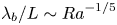

The structure of the flow is depicted in figure 3.
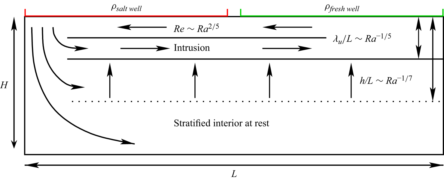
Figure 3. Schematics showing the intrusion regime of Chiu-Webster et al. (Reference Chiu-Webster, Hinch and Lister2008) and the scaling exponents reported in the present study. Note that the Hughes et al. regime would correspond to  $h=H$ and the intrusion flow scale to
  $\lambda _b/L\sim Ra^{-1/5}$ while the Rossby regime would correspond to
  $\lambda _u \approx H$.
3.4. Hughes et al.'s (Reference Hughes, Griffiths, Mullarney and Peterson2007) laminar boundary-layer/turbulent plume regime $I^+_u$

Increasing  ${Ra}$ and for intermediate
  ${Pr}$, the momentum boundary layer becomes progressively thinner compared with the thermal boundary layer. In this case, it is the thermal boundary layer that drives the dynamics and leads to a turbulent plume and a circulation that spans the entire depth of the domain. This particular case was theorized by Hughes et al. (Reference Hughes, Griffiths, Mullarney and Peterson2007) with a plume model inside a filling box. Here, we recast their model according to the Shiskina–Grossmann–Lohse (SGL) theory (i.e. see the plume model definition (2.15)–(2.20) in Hughes et al. Reference Hughes, Griffiths, Mullarney and Peterson2007) and the dissipation in the boundary layer is balanced by the ratio between the thermal and momentum boundary layers
  $\lambda _b/\lambda _u$ according to
 \begin{equation} \overline{\epsilon_{u}}_{HGMP} \sim\nu\frac{U^2}{\lambda^2_u}\frac{\lambda_u}{H}\frac{\lambda_b}{\lambda_u}= \nu^{3}H^{-4}{Re}^{5/2}{Pr}^{-1/2}, \end{equation}
where the dissipation now scales with the thickness of the thermal layer and is given by  $\overline {\epsilon _{u}}\sim \nu U^2/(\lambda _b L)$. Combining (3.2), (3.8) and (3.10) we obtain
 $$\begin{gather} {Re}\sim{Ra}^{2/5}{Pr}^{-3/5}, \end{gather}$$
 $$\begin{gather}{Nu}\sim{Ra}^{1/5}{Pr}^{1/5}. \end{gather}$$
Such a regime is denoted as  $I^+_u$ and was first observed in the experiments of Mullarney et al. (Reference Mullarney, Griffiths and Hughes2004) and Wang & Huang (Reference Wang and Huang2005), and later confirmed in the direct numerical simulations of Gayen et al. (Reference Gayen, Griffiths and Hughes2014).
3.5. The Shishkina & Wagner (Reference Shishkina and Wagner2016) laminar regime $I^*_l$

At low  ${Ra}$ and for large
  ${Pr}$ and/or large aspect ratio
  $\varGamma$, the thickness of the momentum boundary layer
  $\lambda _u$ extends over the depth of the domain, giving
  $\lambda _u=H$. The relation (3.5) becomes
 \begin{equation} \overline{\epsilon_{u}}_{SW} \sim\nu\frac{U^2}{H^2}= \nu^{3}H^{-4}{Re}^{2}. \end{equation}
This expression is equivalent to the dissipation of a pressure-driven laminar channel-type flow. Because this regime requires that the boundary layers span the entire domain, this flow may only be observed for high aspect ratio domains or small Rayleigh numbers, which enforce confinement and is the case in the present study. Combining (3.2), (3.8) and (3.12), we obtain the laminar scaling derived in Shishkina & Wagner (Reference Shishkina and Wagner2016)
 $$\begin{gather} {Re}\sim{Ra}^{1/2}{Pr}^{-1}, \end{gather}$$
 $$\begin{gather}{Nu}\sim{Ra}^{1/4}{Pr}^{0}, \end{gather}$$
denoted as  $I^*_l$, where Beardsley & Festa (Reference Beardsley and Festa1972) first attempted numerical simulations. It is interesting to note that this scaling is similar to the analysis of Gramberg et al. (Reference Gramberg, Howell and Ockendon2007) in which the return flow takes place along the bottom layer and may be applicable when the boundary layer spans the entire height of the domain. Note that Rossby (Reference Rossby1998) also observed a steeper scaling than
  $Nu\sim Ra^{1/5}$ in his numerical simulations for low
  $Ra$ (see p. 248 in Rossby Reference Rossby1998) and similarly in the work of Siggers, Kerswell & Balmforth (Reference Siggers, Kerswell and Balmforth2004).
Note that the Shishkina & Wagner (Reference Shishkina and Wagner2016) regime  $I^*_l$ is expected to occupy the full depth of the domain in figure 3 and we anticipate that the intrusion regime will occur for a larger
  ${Ra}$ than the
  $I^*_l$ regime.
3.6. The role of the aspect ratio and finite width
The effect of the domain aspect ratio was also analysed by Chiu-Webster et al. and was reanalysed by Sheard & King (Reference Sheard and King2011), who reached similar conclusions: for small aspect ratios  $\varGamma <1$ and large enough Rayleigh numbers, the flow follows the
  $I_l$ regime. For
  $\varGamma \geqslant 2$ and
  $Pr\gg 1$, the Nusselt-number dependence exhibits a slightly steeper scaling and agrees with the conclusions of Shishkina & Wagner. Note that these theories did not consider the effect of sidewalls and thus the importance of finite or closed domains. This particular point remains an open question and will not be addressed in this work.
3.7. Turbulent regimes at high Prandtl numbers
Most of the existing work in HC at high Pr considers flows driven by laminar-type scaling laws, dominated by the behaviour of the boundary layer, except for an analogue of HC by Griffiths & Gayen (Reference Griffiths and Gayen2015) and Rosevear et al. (Reference Rosevear, Gayen and Griffiths2017). In a recent study, they considered a spatially periodic forcing at the conducting boundary with a short wavelength compared with the depth of the domain. Reference Passaggia and ScottiPart 1 identifies a similar transition, but the present study could not achieve the necessary Rayleigh numbers (up to  $Ra^{22}$) to allow us to observe the transition to a such regime.
4. Experimental results
4.1. Time-scale analysis
We begin by considering the time scale over which a high-Pr HC system will reach a steady state. Clearly, such experiments are possible if the actual time scale is considerably shorter than the purely diffusive time  $\tau _d\sim \kappa ^{-1}H^{2}$, which is close to a year for the largest tank used in our experiments. As we shall see, convection considerably shortens the transient by stirring the top layer or by entrainment and detrainment in the plume, as seen in figures 2 and 3. The amount of buoyancy transported along the horizontal direction over the distance
  $L$ is controlled by the streamfunction
  $\varPsi$ and the thickness of the pycnocline. Using the scaling laws derived in the previous section,
 \begin{equation} \varPsi_{max}/\kappa \sim {Ra}_f^{1/6} \quad \mbox{and} \quad \lambda_b / L \sim {Ra}_f^{-1/6}, \end{equation}
and substituting relation (2.3) together with the definitions of the Nusselt and the Reynolds number, the scaling laws become
 \begin{equation} {{Re} \sim \varPsi_{max}/\kappa \approx c_1 {Ra}^{1/5} \quad \mbox{and} \quad {Nu}\sim \left(\lambda_b / L\right)^{-1} = c_2 {Ra}^{1/5}. } \end{equation}
 The prefactors  $c_1$ and
  $c_2$ are obtained fitting the theory from experimental data. In this HC set-up, Griffiths et al. (Reference Griffiths, Hughes and Gayen2013) showed that the stable layer acts as a buffer to adjustments or imbalances imposed at the boundaries. In the stably stratified region, the conductive flux is the only mediator to mass, and thus buoyancy transfers. In the case of an imposed buoyancy flux, the initial state has an interior buoyancy
  $b_1$ and a total buoyancy flux input
 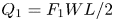 $Q_1 =F_1 WL/2$ through the membrane with the denser fluid located above the tank. In the initial steady state, the flux withdrawn is equal to the input
  $Q_1$. Consider the case of a flux boundary condition (Neumann). At
  $t=0$ let the negative buoyancy input increase from
  $Q_1$ to
  $Q_2 = Q_1 + \delta Q$. Previous experiments and numerical solutions show that the boundary buoyancy input in the equilibrium state is carried to the bottom of the tank by the endwall plume (shown in figure 2, see also Mullarney et al. Reference Mullarney, Griffiths and Hughes2004; Stewart et al. Reference Stewart, Hughes and Griffiths2012; Gayen et al. Reference Gayen, Griffiths, Hughes and Saenz2013; Passaggia et al. Reference Passaggia, Hurley, White and Scotti2017). Therefore, we can assume that, in the transient flow, the ‘unbalanced’ buoyancy input (in excess of that in the equilibrium state) will also be carried to the bottom of the domain by the plume, where it spreads laterally across the bottom of the tank before being displaced upward by the continuing plume transport. Thus, the interior buoyancy
  $b(t)$ decreases, leading to an increase in buoyancy difference
  $b - b_f$ across the boundary layer and an increasing rate of conductive negative buoyancy withdrawal, which we write as
  $Q = Q_1 + Q_0(t)$. The rate of change in buoyancy
  $\tilde {b}$ averaged over the interior assuming that
  $\lambda _b \ll H$ obeys
 \begin{equation} LWH\frac{\mbox{d} \tilde{b}}{\mbox{d} t} = \delta Q - Q'(t), \end{equation}
where  $\tilde {b}(t)$ is the spatial average of the buoyancy over the domain. The imbalance vanishes at large times, when
  $Q'(t) \rightarrow \delta Q$. For quasi-steady conduction in the boundary layer over the buoyant half-part of the top, the rate of buoyancy withdrawal is
 \begin{equation} Q_{1}+Q^{\prime}(t) \approx \beta \kappa\left(\tilde{b}-b_{f}\right) L W / 2 \lambda_b, \end{equation}
over the half of the domain  $L/2$ and we write the gradient at the boundary as
  $\langle \mbox {d}b/\mbox {d}z \rangle _{z=H} \approx \beta {(\tilde {b}-b_f)}/{\lambda _b}$ (the factor 2 stems from the fact that freshening occurs only over half of the domain). In their analysis, Griffiths et al. (Reference Griffiths, Hughes and Gayen2013) did not separate the momentum BL (
 $\lambda _u$) from the buoyancy (thermal in their case) BL (
 $\lambda _b$) and defined
  $\beta$ so that 95 % of the overall buoyancy difference lies in the BL. The constant was evaluated from direct numerical simulation (DNS) for
  $\beta \approx 1.4$ at
  ${Pr}\approx 5$. Since the flow is essentially laminar in the stably stratified layer and transitional in the statically unstable zone, the constant
  $\beta$ can be seen as the ratio between the momentum BL and the buoyancy BL such that
 \begin{equation} \beta \approx \frac{\lambda_u\langle \mbox{d}b/\mbox{d}z \rangle_{z=H}} {{(\tilde{b}-b_f)}} \approx c_4 \lambda_u {Nu} \approx c_4 {Re}^{-1/2} {Nu} \approx c_4 {Pr^{\alpha}}, \end{equation}
where  $\alpha =1/2$ in the Rossby and Shishkina & Wagner regimes while
  $\alpha =4/10$ for the Hughes’ et al. regime. Applying the above to the results of Griffith et al., we obtain
  $c_4\approx 0.74$, while
  $c_2\approx 0.71$ was obtained from figure 4. At large time, the system approaches the final equilibrium state, in which
  $\tilde {b} = b_2$ and
 \begin{equation} Q_{1}+\delta Q \approx \beta \kappa\left(b_{2}-b_{f}\right) L W / 2 \lambda_b. \end{equation}
Taking  $\lambda _b$ as constant for small changes in boundary conditions and combining (4.3)–(4.4) gives the interior buoyancy
 \begin{equation} \tilde{b} \approx b_{1}+\delta b\left(1-\exp({-\beta \kappa t / 2 \lambda_b H})\right), \end{equation}
which exponentially approaches a final equilibrium temperature  $b_2$, the magnitude of the resulting change being
 \begin{equation} \delta b=b_{2}-b_{1}=2 \lambda_b \delta Q /\left(\beta \kappa L W\right)=\lambda_b \delta F /\left(\beta \kappa\right). \end{equation}
In normalized form, the deviation from the final equilibrium is
 \begin{equation} \mathcal{B}=\left(\tilde{b}-b_{2}\right) /\left(b_{1}-b_{2}\right) \approx \exp({-\beta \kappa t / 2 \lambda_b H}). \end{equation}
The imposed flux condition causes the box to equilibrate to the new conditions on the exponential time scale  $\tau _{F} \approx \beta \lambda _b H / \kappa$. The Rayleigh-number scaling (4.2a,b) justifies our assumption of constant
  $\lambda _b$ for modest changes in boundary conditions. It also implies a more rapid adjustment for larger
  ${Ra}_f$ such that
 \begin{equation} \kappa \tau_{F} / H^{2} \approx(2 / \beta)(\lambda_b / H) \approx \varGamma \left (2 c_2 / c_4\right) {R a}^{-1 / 5}{Pr}^{-1/2}. \end{equation}
The evolution of  ${Ra}_f$ (or equivalently
  $Nu$) in each well is shown in figure 5, where both the source and the sink of buoyancy reach the same value, which implies that the flow has reached a steady state and that no significant evaporation is taking place. Note that the time scale was not non-dimensionalized to reflect the duration of the experiments in different tanks. For example, in the small tank, the diffusion time scale for salt
  $\tau _d\sim \kappa ^{-1}H^{2}\approx 5$ days, while in the largest tank, it would be nearly one year. Although four days are necessary to obtain a steady state in the small tank, which already suggests that a viscous scaling will be at play, it only took a month to reach a steady state in the larger tank, confirming that vigorous convection at the surface is present. Under the conditions of the experiments reported in this paper, we find
  $\kappa \tau _{F} / H^{2} \approx [9.7, 201]\times 10^{-3}$ (or
  $\tau _{F} \approx [1.2 \times 10^{3}, 5.1 \times 10^{3}] \mathrm {s}$). Sample results are shown for the
  $L=0.5$ m tank in figure 5(a) and for the
  $L=2$ m tank in figure 5(b) where all cases were run for at least
  $100$ times the flux time scale
  $\tau _f$ highlighted in the analysis. Note that
  $\tau _f$ was also used to estimate the time it would take between the time the particles were inserted and the collection of PIV data.

Figure 4. Flux-Rayleigh number  ${Ra}_f$ as a function of
  ${Ra}$ plotted against the laminar scaling
  ${Ra}_f\approx c_2{Ra}^{6/5}$ where
  $c_2=0.71$.

Figure 5. Temporal evolution of the flux-Rayleigh value in the small tank  $L=0.5$ m (a) and the medium tank
  $L=2$ m (b) over time. Here, time is rescaled with respect to the diffusion time scale
  $\tau _d$. Blue curves represent the evolution of fresh-water wells, and red curves represent the evolution of salt-water wells.
As suggested by Rocha et al. (Reference Rocha, Constantinou, Smith and Young2020), this time scale may prove to be short compared with the actual time necessary to establish a complete steady state, since the bulk and the boundary layers may be characterized by different time constants. In their numerical simulations, they found that a complete steady state was achieved for a time scale  $\tau \approx 0.15\tau _d$. Note that these experiments were in a transitional regime at
  ${Pr}=1$ and that our experiments were carried out until the measured fluxes were balanced (at least
  $0.15\tau _d$), confirming that steady states were reached for each experiment.
4.2. Steady states and local measurements
The PIV of the full domain could only be performed for the smaller tanks, and we resorted to another alternative to estimate the Reynolds and Péclet numbers for the larger tanks. Since we work in tanks with a large aspect ratio (i.e.  $\varGamma =16$), we propose an estimate for the Reynolds number, which can be obtained from measurements of the local streamfunction in the middle of the domain. At first order, the Reynolds number is approximated as
 \begin{equation} {Re}\approx \frac{L^2}{H\lambda_u\nu}\max(\varPsi(z))|_{x=L/2,y=W/2}, \end{equation}
where the lateral effects were neglected. The Péclet number can then be defined as  $Pe = Pr Re$. This is consistent with our experimental observation of the streamfunction measured with PIV (figure 6a).

Figure 6. Snapshots of the mean streamfunction for (a)  ${Ra}=1.19\times 10^{13}$ and (b)
  ${Ra}=4.48\times 10^{13}$ corresponding to trials
  $2$ and
  $5$ in table 1 showing the progressive clustering of the circulation beneath the forcing boundary. These figures were obtained from PIV, integrating the mean velocity to obtain the streamfunction
  $\varPsi$, which is then non-dimensionalized using (4.2a,b).
Rescaled density profiles, measured in the centre of the domain  $x=L/2$ are shown in figure 7(a) for most of the range of Rayleigh numbers reported in the present study. As
  $Ra$ increases, the flow exhibits the same behaviour as seen in the experiment of Mularney et al. but with a thinning of the pycnocline and an increase in the dense, well-mixed fluid, filling the bottom and the centre of the domain.

Figure 7. (a) Normalized density profiles  $({\rho (z)-\rho _{min}})/({\rho _{max}-\rho _{min}})$ and (b) streamfunction
  $\varPsi (z)$ non-dimensionalized using (4.2a,b) and calculated from averaged PIV data and rescaled with Rossby scaling as suggested by Chiu-Webster et al., measured in the middle of the tank (
 $x=L/2$).
The profiles of the streamfunction normalized with the Rossby scaling and collected at the same location are shown in figure 7(b) for the same values of  $Ra$ as in figure 7(a). The two regimes identified with the analysis of the Nusselt-number scaling can also be observed with the evolution of the streamfunction as a function of
  $Ra$. The maximum of the streamfunction becomes progressively closer to the forced boundary at
  $z=H$. It should be noted that the location of the streamfunction approaches the buoyancy–forced boundary when
  ${Ra}\gtrsim 10^{15}$ while the flow is essentially at rest in the core of the domain. This observation follows the results of the experiments of Wang & Huang (Reference Wang and Huang2005) performed at
  $Pr\approx 8$. Note that Wang & Huang also reported a regime transition, but did not see a change in exponents across each regime. We emphasize that, in the case of Wang & Huang, the aspect ratio was small
  $\varGamma =1.3$ and of width
  $W/L\approx 1/8$, while in our experiments
  $\varGamma \approx 16$ and
  $W/L\approx 1/16$. We therefore witness the transition from a confined flow to the flow with an interior at rest, as recently described in Shishkina & Wagner (Reference Shishkina and Wagner2016). Note that a small recirculation region is observed in figure 7(b) at the bottom of the tank (shown by a small bump in the streamfunction), which was present in almost all experiments except for the smaller tank. We hypothesize that this feature, not present in the Wang & Huang experiments, is possibly due to undesirable heating from the bottom of the tank.
Chiu-Webster et al. (Reference Chiu-Webster, Hinch and Lister2008) derived asymptotic solutions to the problem of very viscous convection, and in particular, the solution for the evolution of the temperature in the core of the domain. In particular, they showed that the temperature (i.e. equivalent to the buoyancy up to a negative multiplicative constant) scaled as
 \begin{equation} b(z) = \frac{c_5}{Ra(z+h)^7}, \end{equation}
where  $h$ is the height of the bulk as defined in figure 3 and
  $c_5$ is a constant, both obtained from fitting the results in figure 7(a) to (4.12). As shown in Chiu-Webster et al., the height
  $h$ derives naturally at first order for the temperature equation in the limit where
  $Pr\rightarrow \infty$, which becomes Laplace equation in this particular limit. Using the results obtained in figure 7(a), figure 8(a) shows that self-similarity can be recovered in the interior and that
  $b(x=L/2,z) \approx c_5 (z+h)^{1/7}$ where
  $c_5=1.9$.

Figure 8. (a) Rescaled normalized buoyancy profiles as defined in (4.12). (b) Rescaled streamfunction profiles showing the self-similar nature of the flow near the upper boundary.
Figure 8(b) shows the values of the streamfunction obtained in 7(b) rescaled with  ${Ra}^{1/5}$ for the vertical direction
  $z$ as in (4.2a,b), and for a large range of Rayleigh numbers. It is worth noting that the streamfunction becomes self-similar in the range
  $(1-z\varGamma ){Ra}^{1/5}=[0,1]$ and
  ${Ra}>10^{15}$, which corresponds to circulating flow. Note that the solution is no longer self-similar where
  $(1-z\varGamma ){Ra}^{1/5}>1$, which justifies the use of (4.12) in the interior, providing further support for the analysis of the regime transitions.
4.3. Scaling analysis
The dependence of  ${Nu}$ and
  $\varPsi _{max}$ (and equivalently
  ${Re}$) on the Rayleigh number
  ${Ra}$ is summarized in figure 9(a–f). Similarly to the analysis in terms of the flux–Rayleigh number, we observe two different scaling exponents (figure 9a): for
  $Ra\lesssim 10^{15}$, the flow exhibits a scaling exponent
  ${Nu}\sim {Ra}^{1/4}$, while for
  $Ra\gtrsim 10^{15}$ the salt uptake rate decreases to exhibit a
  $Nu\sim Ra^{1/5}$-type scaling. The same compensated plot is shown in figure 9(b), where the difference between the two scalings is only a factor
  $2.5$ at
  $Ra=7.11\times 10^{16}$ over the full dynamic range of our experiments and underlines the importance of the large Rayleigh-number ranges to differentiate between the two scaling laws.

Figure 9. The (a)  ${Ra}$ and (b) rescaled-
 ${Ra}$ dependencies of the Nusselt number. (c) Buoyancy boundary-layer thickness
  $\lambda _b$ and (d) momentum boundary thickness
  $\lambda _u$, compared with the theory of Chiu-Webster et al. (Reference Chiu-Webster, Hinch and Lister2008) (red) and Shishkina & Wagner (Reference Shishkina and Wagner2016) (black). (e) Bulk thickness
  $h/H$ compared with the theory of Chiu-Webster et al. (f) Maximum of the streamfunction
  $\varPsi _{max}$ as a function of
  ${Ra}$ and the linear regression over the full range.
Based on figure 7(a,b), we extrapolate the thickness of both the kinetic boundary layer  $\lambda _u$ and the pycnocline thickness
  $\lambda _b$. The former is given by the location of the maximum of the streamfunction
  $\max {(\varPsi (z))}$, the latter was extrapolated using the height of the fiftieth percentile of the rescaled density profile. The evolution of the buoyancy boundary layer is reported in figure 9(c) and shows again two different behaviours. For
  $Ra<10^{15}$, the buoyancy boundary-layer thickness decreases and follows a
  $Ra^{-1/4}$ scaling. At
  $Ra \approx 10^{15}$, we observe a regime change where the thickness now decreases so that
  $Ra^{-1/4}$. A similar behaviour is observed in figure 9(d), where the thickness of the kinetic boundary layer
  $\lambda _u$ is reported. For
  $Ra\lesssim 10^{15}$, the kinetic boundary layer saturates at
  $\lambda \approx 0.4$, which is in agreement with the study of Shishkina & Wagner (Reference Shishkina and Wagner2016). Past
  $Ra\gtrsim 10^{15}$, we recover the Rossby scaling for
  $\lambda _u\sim Ra^{-1/5}$ and, together with the bulk reduction, this suggests that we are observing the intrusion-type flow studied by Chiu-Webster et al. (Reference Chiu-Webster, Hinch and Lister2008).
We confirm this claim in figure 9(e), where the thickness of the core  $h\varGamma$ is shown as a function of the Rayleigh number. This thickness was measured fitting (4.12) from the data reported in figure 7(a), as shown in 8(a). Using their plume theory, Chiu-Webster et al. (Reference Chiu-Webster, Hinch and Lister2008) showed that the thickness of the bulk decreases as
  $Ra^{-1/7}$. This scaling is compared with the data points that suggested such behaviour for
  $Ra\gtrsim 10^{15}$. Although based only on a few data points, we may be witnessing the intrusion regime described by Chiu-Webster et al. (Reference Chiu-Webster, Hinch and Lister2008).
Conclusions from the maximum of the streamfunction shown in figure 9(f) are more difficult to draw. From Shishkina & Wagner (Reference Shishkina and Wagner2016), we would expect a Reynolds-number scaling as  $Re\sim Ra^{1/2}$ and
  $\lambda _u\sim {Ra}^{1/2}$, which results in
  $\varPsi _{max}\sim {Ra}^{1/4}$. For larger values of
  $Ra$, we would expect
  ${\varPsi }_{max} \sim Ra^{1/5}$, similar to the Rossby scaling. A linear regression across the entire data set provides
  $\max {\varPsi }\sim Ra^{0.225}$, which lies between the
  $1/4$ exponent expected from the Shishkina & Wagner (Reference Shishkina and Wagner2016) analysis and the
  $1/5$ predicted in Chiu-Webster et al. (Reference Chiu-Webster, Hinch and Lister2008). Note that all data points for the maximum of the streamfunction were not reported since PIV proved difficult near the boundary for the largest buoyancy inputs in the wells, in particular in the smaller tank.
The present experimental results, based on a regime similar to Shishkina & Wagner (Reference Shishkina and Wagner2016), suggest a transition from the  $I_l^*$ regime to the
  $I_u$ intrusion regime of Chiu-Webster et al. (Reference Chiu-Webster, Hinch and Lister2008) for Prandtl numbers one order of magnitude larger than the direct numerical simulations of Shishkina & Wagner (Reference Shishkina and Wagner2016) and Rossby (Reference Rossby1965), and Rayleigh numbers up to seven orders of magnitude larger than previous experiments and direct numerical simulations for similar Prandtl numbers. In the next subsection, we discuss the present results with the results at intermediate and low Prandtl numbers presented in Reference Passaggia and ScottiPart 1 We propose an updated regime transition diagram of horizontal convection.
5. Completing the regime diagram of natural horizontal convection
In this section, we summarize the different HC regimes that were observed in the  $({Ra, Pr})$ space in the present work and Reference Passaggia and ScottiPart 1 (Passaggia & Scotti Reference Passaggia and Scotti2024), together with all the results that we could gather from the literature on HC (figure 10(a)–(b)). This section aims at extending the regime diagram in Hughes et al. (Reference Hughes, Griffiths, Mullarney and Peterson2007) and the limiting regimes provided in Shishkina et al. (Reference Shishkina, Emran, Grossmann and Lohse2017).
We first provide a nomenclature for the different regimes:
(i)
nearly conducting (i.e. ${Nu}\sim \mathrm {const.}$);(ii)
laminar;(iii)
transitional (only turbulent in the plume);(iv)
enhanced transitional (only turbulent in the BL but never observed);(v)
both boundary layers and plume are turbulent.


Figure 10. (a) Summary combining of all calculations found in the literature from experiments and DNS on HC together with the present experiments ( $\blacksquare$, magenta) and DNS from Reference Passaggia and ScottiPart 1 (Passaggia & Scotti Reference Passaggia and Scotti2024) (
 $\bullet $, blue). The plotted results also include: (- -) (blue dashed line) Rossby (Reference Rossby1965), (- -) (orange dashed line) Miller (Reference Miller1968), Beardsley & Festa (Reference Beardsley and Festa1972) (—) (black dashed line), Paparella & Young (Reference Paparella and Young2002) (red transparent square), Siggers et al. (Reference Siggers, Kerswell and Balmforth2004) (transparent yellow square), Mullarney et al. (Reference Mullarney, Griffiths and Hughes2004) (black dashed line), Wang & Huang (Reference Wang and Huang2005) (brown line), Sheard & King (Reference Sheard and King2011) (magenta horizontal line), Gayen et al. (Reference Gayen, Griffiths and Hughes2014) (green lines), Shishkina et al. (Reference Shishkina, Emran, Grossmann and Lohse2017) (transparent purple square with borders) and Reiter & Shishkina (Reference Reiter and Shishkina2020) (- -) (red horizontal dashed lines). (b) Phase diagrams in the
  $({Ra}, {Pr})$ plane that combine the present results with Reference Passaggia and ScottiPart 1 (Passaggia & Scotti Reference Passaggia and Scotti2024) at low Prandtl numbers, showing the different regimes of HC for the present flow geometry. Note that all of the above results considered no-slip boundary conditions, except for the results reported in Passaggia & Scotti (Reference Passaggia and Scotti2024). In addition, dashed lines and rectangles with borders denote experiments or simulations with sidewalls.
Additional subscripts and superscripts are identified as:
(i)
for large Prandtl numbers;(ii)
for low Prandtl numbers;(iii)
when essentially controlled by the aspect ratio;(iv)
when essentially controlled by the plume dynamics.
We begin with the conducting regime ![]() , which was analysed in Siggers et al. (Reference Siggers, Kerswell and Balmforth2004), Chiu-Webster et al. (Reference Chiu-Webster, Hinch and Lister2008) and, more recently, by Sheard & King (Reference Sheard and King2011), where
, which was analysed in Siggers et al. (Reference Siggers, Kerswell and Balmforth2004), Chiu-Webster et al. (Reference Chiu-Webster, Hinch and Lister2008) and, more recently, by Sheard & King (Reference Sheard and King2011), where  $Nu\sim Ra^0 Pr^0$. The onset is independent of the Prandtl number, the transition is smooth and weakly affected by the aspect ratio
  $\varGamma$ and occurs when
  $Ra\approx 10^{3}$. The conducting regime neighbours the
 ![]() regime which follows the scaling in (3.12a) or the
regime which follows the scaling in (3.12a) or the ![]() regime in (3.4a) depending on the aspect ratio. The transition was found to not depend on
regime in (3.4a) depending on the aspect ratio. The transition was found to not depend on  $Ra$, consistent with the results reported in the literature (Siggers et al. Reference Siggers, Kerswell and Balmforth2004; Sheard & King Reference Sheard and King2011).
The connection between the laminar regimes ![]() and
and ![]() is determined by matching the Reynolds numbers in these neighbouring regimes. From (3.12b) and (3.4b), we obtain the slope of the transition region between the regimes
is determined by matching the Reynolds numbers in these neighbouring regimes. From (3.12b) and (3.4b), we obtain the slope of the transition region between the regimes  $I^*_{l}$ and
  $I_l$, which is
  ${Pr}\sim {Ra}^{1/2}$. This transition is smooth (Shishkina et al. Reference Shishkina, Emran, Grossmann and Lohse2017), but is strongly affected by both the aspect ratio of the domain and the type of boundary conditions. Note that the free-slip boundary conditions make it easier to observe this regime. Results from Rossby (Reference Rossby1998), Shishkina & Wagner (Reference Shishkina and Wagner2016) and the present work confirm that high aspect ratio domains are necessary to observe the
  $I^*_l$ regime. With increasing aspect ratios, the boundary layer becomes increasingly thick with respect to depth
  $H$ and eventually covers the entire depth of the domain for a small enough Rayleigh number. To reflect this dependence in the regime diagram, this transition is marked by a dashed line because of its strong aspect ratio dependence. The present dashed line was approximated as a fit from the present results and Shishkina et al. for aspect ratios
  $\varGamma \sim O(10)$ but the reader should keep in mind that the present landscape should include a third dimension,
  $\varGamma$, to be complete.
As both  ${Ra}$ and
  $Pr$ increase, the Rossby regime progressively evolves towards the intrusion regime studied by Chiu-Webster et al. (Reference Chiu-Webster, Hinch and Lister2008) and observed for large Rayleigh numbers in this study. This regime has the same dependence on the Prandtl and Reynolds numbers as the laminar Rossby regime, but the flow has a significantly different structure. We therefore propose to name this flow
 ![]() to remain consistent with the Shishkina et al. (Reference Shishkina, Grossmann and Lohse2016) nomenclature.
to remain consistent with the Shishkina et al. (Reference Shishkina, Grossmann and Lohse2016) nomenclature.
As  $Ra$ increases and for
  $Pr\approx O(1)$, we observe the
 ![]() regime of Hughes et al. (Reference Hughes, Griffiths, Mullarney and Peterson2007). As shown in Gayen et al. (Reference Gayen, Griffiths and Hughes2014), the transition for increasing
regime of Hughes et al. (Reference Hughes, Griffiths, Mullarney and Peterson2007). As shown in Gayen et al. (Reference Gayen, Griffiths and Hughes2014), the transition for increasing  $Ra$ is not smooth, and this flow exists only over a small region of the regime diagram. The flow transitions to
 ![]() when
when  $Pr$ increases and appears at constant
  $Pr$. This can be shown by equating (3.4b) and (3.10b) and this transition from
 ![]() to
to ![]() was highlighted by Gayen et al. (Reference Gayen, Griffiths and Hughes2014) (see p. 712).
was highlighted by Gayen et al. (Reference Gayen, Griffiths and Hughes2014) (see p. 712).
For low  $Pr$, a sharp transition from
 ![]() to
to ![]() was reported in Passaggia & Scotti (Reference Passaggia and Scotti2024). This transition occurs at
was reported in Passaggia & Scotti (Reference Passaggia and Scotti2024). This transition occurs at  $Pr\sim Ra^{1/2}$ across a bifurcation of the flow. Note that, similarly to the high-
 $Pr$ regimes, the circulation shrinks as
  $Pr$ decreases. Also, note that the transition from
 ![]() to
to ![]() has a complex shape and is strongly dependent on the aspect ratio
has a complex shape and is strongly dependent on the aspect ratio  $\varGamma$.
The last transition appears as the Rayleigh number increases and was first observed at  ${Ra}\approx 10^{11}$ and
  ${Pr}\approx 0.1$. The
 ![]() regime transitions to the limiting regime
regime transitions to the limiting regime ![]() . This transition was smooth and marks the appearance of a first limiting regime for asymptotic
. This transition was smooth and marks the appearance of a first limiting regime for asymptotic  $Ra$, consistent with the zeroth law of turbulence where the Reynolds and Nusselt numbers are driven by turbulent-scaling arguments. The transition from
 ![]() to
to ![]() appears as
appears as  $Ra \sim Cst$ as reported in Passaggia & Scotti (Reference Passaggia and Scotti2024). The separation between the regime's argument is more difficult to draw since we have not been able to identify the transitions between the regimes directly from previous works. In addition, regime
 ![]() displays logarithmic Reynolds-number corrections for the Reynolds and the Nusselt number, which lead to the scaling
displays logarithmic Reynolds-number corrections for the Reynolds and the Nusselt number, which lead to the scaling  $Pr\sim Ra^{1.66}\mathcal {L}({Re}^{16})$, which is strongly dependent on the Reynolds number. This is not too surprising since transition to turbulence is expected to be Reynolds-number dependent (Lohse & Shishkina Reference Lohse and Shishkina2023). Furthermore, the Prandtl-number dependence on the log correction could not be verified in the work of Passaggia & Scotti (Reference Passaggia and Scotti2024), which leaves questions open regarding the complete understanding of this flow regime and its transitions. Another alternative would be to use the values reported in table 2 and match the Nusselt number between
 ![]() and
and ![]() . Still, the scaling law depends again on the actual values of the Reynolds number and would provide, for this particular case,
. Still, the scaling law depends again on the actual values of the Reynolds number and would provide, for this particular case,  $Pr\sim Ra^{-0.115}$. Note that the same conclusion applies to the transition between
 ![]() and
and ![]() . For these reasons, the transitions region is shown by a red dashed line and remains a matter for further investigation. All the regimes summarized in the section are provided in table 2.
. For these reasons, the transitions region is shown by a red dashed line and remains a matter for further investigation. All the regimes summarized in the section are provided in table 2.
Table 2. List of scaling laws obtained for the Nusselt- and Reyolds-number dependencies across different regimes. The prefactors and the scalings with an asterisk are estimated from the numerical simulations. All other exponents are derived from theoretical considerations.

Regarding the ultimate regime ![]() predicted in Siggers et al. (Reference Siggers, Kerswell and Balmforth2004) and Shishkina et al. (Reference Shishkina, Emran, Grossmann and Lohse2017), where
predicted in Siggers et al. (Reference Siggers, Kerswell and Balmforth2004) and Shishkina et al. (Reference Shishkina, Emran, Grossmann and Lohse2017), where  $Nu \sim Ra^{1/3}Pr^{-2/3}$ and
  $Re \sim Ra^{1/3}Pr^{1/3}$, the bound on the Richardson number in the stratified boundary layer, derived in Passaggia & Scotti (Reference Passaggia and Scotti2024), shows that this regime seems unattainable as long as the boundary is considered as perfectly flat (Lohse & Shishkina Reference Lohse and Shishkina2023), (i.e. for instance without roughness elements). This particular point deserves more investigation and whether such a regime can be attained is of utmost importance for geophysical applications. Nevertheless, in the present academic configuration assuming perfectly flat boundaries, the regime
 ![]() seems to be the limiting regime attainable at very large Rayleigh numbers.
seems to be the limiting regime attainable at very large Rayleigh numbers.
This updated regime diagram covers, to the best of our knowledge, all previous DNS and experimental studies performed on HC. The last regime observed at high Rayleigh numbers is a turbulent-dominated regime in the bulk, which satisfies the zeroth law of turbulence Shishkina et al. (Reference Shishkina, Grossmann and Lohse2016). The resulting flow characteristics at high Rayleigh numbers and all Prandtl numbers are an intensified turbulent near-surface circulation which follows Sandström's original inference, Jeffrey's argument and the PY bound on dissipation. They argued that the flow generated by HC would result in an essentially stagnant pool of water with little to no flow in the core and an intensified turbulent circulation localized near the differentially heated boundary. Our results show that limiting regimes at all Prandtl numbers for large Rayleigh numbers inevitably lead to such a scenario.
6. Conclusions
This work considers laboratory experiments of HC at high Prandtl and high Rayleigh numbers. This work aims to explore a part of the regime diagram that has not yet been explored in previous studies. Related experimental work at high Prandtl numbers dates back to the original work Rossby (Reference Rossby1965) and Miller (Reference Miller1968) more than half a century ago. Instead of differential heating, where increasing the Prandtl number is achieved by increasing the viscosity of the working fluid, we consider solutal convection and use a permeable dialysis membrane to allow for a mass/salinity flux through the forcing boundary while ensuring a no-flow/no-slip boundary condition in a high aspect ratio and narrow domain.
Experiments that span four orders of magnitude in the Rayleigh number while keeping the Prandtl number constant are performed. This allows for measuring two known regimes, already identified in the literature in natural HC at higher Prandtl numbers but for much larger values of the Rayleigh number (up to seven orders of magnitude larger) than previously reported. We provide experimental evidence of the laminar regime identified by Shishkina & Wagner (Reference Shishkina and Wagner2016) where the recirculating flow, and thus the boundary layer, has the same domain size. This regime leads to a regime  $Nu \sim Ra^{1/4}$ that is consistent with direct numerical simulations at high
  $Pr$ and lower
  $Ra$, where the effects of confinement enhance the amount of laminar dissipation and provide a mechanism for a heat transfer larger than previously theorized by Rossby (Reference Rossby1965) for small aspect ratio domains. Increasing further the Rayleigh number beyond
  $Ra \gtrsim 10^{15}$ and for Prandtl numbers
  $Pr\approx 610$, the flow exhibits a transition back to the Rossby regime as the boundary becomes progressively thinner. Experimental evidence of this regime is made possible following the work of Chiu-Webster et al. (Reference Chiu-Webster, Hinch and Lister2008), who analysed HC in the limit of asymptotically large Prandtl numbers, also known as very viscous horizontal convection. This regime is also known as the intrusion regime (Hughes & Griffiths Reference Hughes and Griffiths2008). It follows the same scaling laws as the original Rossby regime, but the structure of the flow is substantially different, with a narrow recirculating/intrusion regime while the core of the flow remains essentially at rest. Using PIV and conductivity measurements at the centre of the domain, we show that for high Rayleigh numbers, the flow follows scaling laws similar to those derived in Chiu-Webster et al.'s asymptotic analysis for the behaviour of the boundary layer and the thickness of the fluid at rest contained in the bulk. Definite conclusions about the magnitude of the streamfunction are harder to draw due to measurement uncertainties but hint at the same arguments.
We report a new regime transition in HC at large Rayleigh and Prandtl numbers. Combining all available evidence, we propose an updated regime diagram that extends the regime diagrams proposed by Hughes & Griffiths (Reference Hughes and Griffiths2008) and more recently by Shishkina et al. (Reference Shishkina, Grossmann and Lohse2016). Seven distinct regimes are mapped for which observations using either DNS or experiments have been confirmed, and the Nusselt-number dependencies are used to draw a complete regime diagram from seven orders of magnitude for the Prandtl number and seventeen orders of magnitude for the Rayleigh number. We also report the six limiting regimes known to this date and, in particular, the transition to the turbulent limiting regime  $IV_u$ for asymptotically large Rayleigh numbers and put an emphasis on the role of the aspect ratio of the domain for large Prandtl numbers. Although it was also shown that the ultimate regime
  $IV_l$ cannot be achieved (Siggers et al. Reference Siggers, Kerswell and Balmforth2004; Passaggia, Scotti & White Reference Passaggia, Scotti and White2016; Passaggia & Scotti Reference Passaggia and Scotti2024), the present regime diagram is consistent with previous studies and reviews and provides a complete parametrization of horizontal convection that can be used for engineering and geophysical applications.
Acknowledgements
The authors thank Dr B. White, Professor D. Lohse, Dr O. Shiskina and three anonymous referees for insightful comments and encouragement.
Funding
This work was supported by the National Science Foundation (grant nos OCE–1155558 and OCE-1736989).
Declaration of interests
The authors report no conflict of interest.


 Open access