


1. Introduction
Impacts between solid bodies occur daily in many natural and industrial processes. For stiff solids, the role of ambient air is negligible; however, compliant solids can be deformed by the lubrication stress in an intervening fluid layer (Rallabandi Reference Rallabandi2024). In this scenario, the lubricant can become entrained, and depending on the contact velocity, the contact area can be reduced (Zheng, Dillavou & Kolinski Reference Zheng, Dillavou and Kolinski2021). Fluid mediated contact between soft bodies governs myriad biological and physical processes, from the adhesion of hydrogel tapes (Xue et al. Reference Xue, Gu, Li, Yu, Yin, Qin, Jiang, Wang and Cao2021), to the haemodynamics of blood cells in the vasculature (Higgins & Mahadevan Reference Higgins and Mahadevan2010) and the rheology of suspensions (Coussot & Ancey Reference Coussot and Ancey1999). Even the mundane act of gripping a dish in the kitchen with our fingers is cushioned by the surrounding air. Despite the ubiquity and importance of fluid-mediated contact between soft solids, the dynamics of contact formation is not fully characterized yet when the cushioning of the intervening fluid cannot be ignored, unlike in the case when it can be (cf. Johnson Reference Johnson1985); indeed, for impact velocities of the order of metres per second, and solids with a shear modulus similar to biological soft tissues, an observed sharp transition of the entrained air suggests a dominant role of elastodynamics, as the deformation rates in the solid transition from super-Rayleigh to sub-Rayleigh speeds (Zheng et al. Reference Zheng, Dillavou and Kolinski2021).
Contact formation between compliant solids in air is analogous to liquid droplet impact; in this context, the lubricating air film generates the first formation of an on-axis dimple before ultimately leading to droplet splashing or spreading (Mandre, Mani & Brenner Reference Mandre, Mani and Brenner2009; Mani, Mandre & Brenner Reference Mani, Mandre and Brenner2010; Kolinski et al. Reference Kolinski, Rubinstein, Mandre, Brenner, Weitz and Mahadevan2012; Riboux & Gordillo Reference Riboux and Gordillo2014; Josserand & Thoroddsen Reference Josserand and Thoroddsen2016; Wu, Cao & Yao Reference Wu, Cao and Yao2021). Theoretical models of ‘air cushioning’ have been developed (Smith, Li & Wu Reference Smith, Li and Wu2003; Hicks & Purvis Reference Hicks and Purvis2010) and validated (Hicks et al. Reference Hicks, Ermanyuk, Gavrilov and Purvis2012) for low-viscosity droplets. It has been reported that the otherwise reasonable, and usually made, assumptions of incompressibility and negligible surface tension break down, and even the air can become rarefied (Mani et al. Reference Mani, Mandre and Brenner2010; Hicks & Purvis Reference Hicks and Purvis2013). Remarkably, if these extra effects did not enter the picture, then normal contact would be mathematically impossible (Wu & Bogy Reference Wu and Bogy2001; Hillairet Reference Hillairet2007). Experiments of highly viscous droplets impacting rigid (Langley, Li & Thoroddsen Reference Langley, Li and Thoroddsen2017) and fluid (Langley & Thoroddsen Reference Langley and Thoroddsen2019) surfaces displayed ‘gliding’ (local hovering around the tip of the droplet's leading edge while the outward regions continue approaching), whereas droplets impacting on a compliant surface entrain a larger amount of air compared to the rigid case (Langley, Castrejón-Pita & Thoroddsen Reference Langley, Castrejón-Pita and Thoroddsen2020). Interestingly, a maximum in air bubble volume has been observed as a function of surface tension (Bouwhuis et al. Reference Bouwhuis, van der Veen, Tran, Keij, Winkels, Peters, van der Meer, Sun, Snoeijer and Lohse2012).
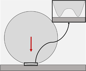
The role played by the mediating air is far less clear for a dynamic soft elastomer impact, and the stress distribution during the impact process remains unknown. The case of fluid-mediated solids interacting with interfaces has been studied extensively by tribologists (Johnson Reference Johnson1985) specializing in elastohydrodynamic lubrication and by chemists interested in convective mass transport (Leal Reference Leal2007). The literature contains examples of a variety of configurations involving solids, ranging from lubrication between a stiff sphere and a rigid interface (Cox & Brenner Reference Cox and Brenner1967), to two spheres immersed in water contacting at relatively low velocity (Davis, Serayssol & Hinch Reference Davis, Serayssol and Hinch1986), a rigid sphere denting an elastic substrate mediated by air (Balmforth, Cawthorn & Craster Reference Balmforth, Cawthorn and Craster2010), a soft interface and a rigid sphere (Verzicco & Querzoli Reference Verzicco and Querzoli2021; Liu et al. Reference Liu, Dong, Jagota and Hui2022), and a rigid interface and a quasi-static soft sphere (Venner, Wang & Lubrecht Reference Venner, Wang and Lubrecht2016; Bertin Reference Bertin2024). Recently, experiments featured soft solid impactors hitting a microscopically flat surface (Zheng et al. Reference Zheng, Dillavou and Kolinski2021). The maximum ‘entrapped air bubble’ was measured at the first instances of contact, and it was shown that its radius grows as a power-law function of the impact velocity up to a maximum value, and then drops suddenly and becomes weakly dependent on impact velocity. It was then suggested that there exist two domains, dominated respectively by elastic and inertial response. In both cases, there is a local viscous pressure ‘build up’ as the air is squeezed, which leads to the formation of a ‘dimple’ around the tip. As time progresses, the dimple expands, and we define the radial position of its edge as the ‘deformation front’ (see figure 1).

Figure 1. (a) General scheme of the local problem. Left: leading edge of a soft solid approaches a rigid surface, trapping a thin film in between. Right: approach is arrested around the axis of the solid by viscous pressures, leading to deformation characterized by vertical length scale  $H$ and radial length scale
  $\mathcal {L}$. (b) Schematic of the impact as modelled at the beginning of the numerical simulation. The coordinate system is set such that the top flat surface of the rigid body (dark grey) is at
  $z=0$. The solid ball (light grey) approaches the surface with initial velocity
  $V$ starting with an initial gap
  $h_0$. The surrounding fluid cushions the impact. (c) Schematic of the lower free surface of the impactor (
 $\partial \varOmega ^{-}$) while approaching the surface. At each time step, the point closer to touchdown is identified, and its radial coordinate is measured (
 $r^*(t)$). The gap between this lowest point and the surface is sometimes said to form a ‘neck’ (Gordillo & Riboux Reference Gordillo and Riboux2022) or a ‘kink’ (de Ruiter et al. Reference de Ruiter, Oh, van den Ende and Mugele2012).
Here, we provide a scaling analysis across a wide range of impact velocities that includes the observed sharp transition between elasticity-dominated and inertia-dominated impacts (Zheng et al. Reference Zheng, Dillavou and Kolinski2021). The scaling analysis complements and provides context for numerical simulations of the impact dynamics, which give additional insight into the pressure in the mediating air film: a pronounced spike in the air pressure emerges as the impact transitions to the inertia-dominant regime. The growth or decay of this pressure spike governs whether the solid will glide over the surface, or get sufficiently close to the surface that contact formation cuts off the gliding process, ultimately reducing the lateral scale of the entrained lubricant.
Unlike some of the literature in impacts of drops (Mandre et al. Reference Mandre, Mani and Brenner2009; Duchemin & Josserand Reference Duchemin and Josserand2011; Gordillo & Riboux Reference Gordillo and Riboux2022; Sprittles Reference Sprittles2024), in this contribution we do not intend to quantify the minimum local thickness of the thin film or the mechanisms that ultimately lead to ‘touchdown’; we focus on understanding the evolution of the lateral extent of the entrapped bubble.
The text is organized as follows. Section 2 presents the geometrical setting, the characteristic scales of the system, and the corresponding regimes. Section 3 briefly introduces our numerical model, and tests the validity of our scaling framework with experiments, simulations and previous literature. Section 4 explains why there is a maximum bubble radius and why its size can change suddenly with model parameters. It also highlights similarities and differences with droplet impacts. We close with final remarks, including the research outlook, in § 5.
2. Scaling for fluid trapping during approach
Consider an elastic solid sphere of radius  $R$, surrounded by a fluid, approaching with velocity
  $V$ a rigid flat surface along its normal; see figures 1(a) and 1(b). In order for the sphere to make contact with the surface, the intervening fluid layer close to the tip must be ejected, resulting in large lubrication pressure. If this pressure is high enough, then it can locally halt the approach of the sphere, causing substantial deformation so that contact will be made on an annulus, with a fluid bubble trapped in the middle. Depending on which mechanism is predominantly responsible for balancing the lubrication stress in the solid (deceleration or deformation), we identify two different regimes. This is sketched in figure 2.

Figure 2. Diagram illustrating how different pressures balancing the lubrication pressure give rise to different regimes (where  $P_{lub} , P_{el} , P_{in}$ represent pressures based on characteristic values of lubrication, elastic forces and inertial forces, respectively).
The condition for fluid pocket formation provides the relation  $\mathcal {L} = \sqrt {R H}$ between the characteristic radius of the dimple
  $\mathcal {L}$, that of the impactor
  $R$, and the characteristic gap size
  $H$ (Smith et al. Reference Smith, Li and Wu2003; see also Appendix A).
For an incompressible fluid film, the lubrication pressure is  $P_{lub} \sim \mu _m' V R /H^2$ (Szeri Reference Szeri2010), where
  $\mu _m' = 12 \mu _m$ (Savitski & Detournay Reference Savitski and Detournay2002), and
  $\mu _m$ is the dynamic viscosity of the mediating fluid. We also define
  $\tau =H/V$ as the characteristic time of the impact final stage. When impactor inertia is dominant, defining
  $\rho _i$ as the solid density, the pressure scale for the solid is
  $P_{in} \sim \rho _i V \mathcal {L} / \tau$, which stems from decelerating the leading edge of the impactor, with characteristic length
  $\mathcal {L}$ and initial velocity
  $V$, over a time span of order
  $\tau$. Balancing
  $P_{in}$ with
  $P_{lub}$ and using the geometrical relation between
  $\mathcal {L}$ and
  $H$, we obtain
 \begin{equation} \mathcal{L}_{in} = R \, St^{{-}1/3},\quad H_{in} = R \, St^{{-}2/3} , \end{equation}
where  $St = \rho _i V R /\mu _m'$ is the particle Stokes number. These results have been reported previously in the literature for droplets (Smith et al. Reference Smith, Li and Wu2003; Mandre et al. Reference Mandre, Mani and Brenner2009).
If elasticity is dominant, then the characteristic value of strain is  $H/\mathcal {L}$, and the pressure scale is thus
  $P_{el} \sim G H/\mathcal {L}$, where
  $G$ is the shear modulus of the impactor. Balancing this pressure with
  $P_{lub}$ yields
 \begin{equation} \mathcal{L}_{el} = (R^4 \mu_m' V/G)^{1/5},\quad H_{el} = (R^{3/2} \mu_m' V/G)^{2/5}. \end{equation}
These results have also been reported previously in the literature (Davis et al. Reference Davis, Serayssol and Hinch1986; Zheng et al. Reference Zheng, Dillavou and Kolinski2021), but we used the shear modulus instead of the equivalent Young's modulus for ease of interpretation of later results, effectively removing an order-one prefactor.
2.1. Transition between elasticity-dominated and inertia-dominated impactor response
We will use the notation  $P_y[x]$ to denote that the characteristic value of the pressure
  $P_y$ is evaluated using scale(s)
  $x$. The crossover between elastic and inertial regimes occurs when
  $P_{in} \sim P_{el}$. We notice that
 \begin{align} \left(\frac{P_{in}[\mathcal{L}_{in}, H_{in}]}{P_{el}[\mathcal{L}_{in}, H_{in}]}\right)^{1/2} = \left(\frac{P_{in}[\mathcal{L}_{el}, H_{el}]}{P_{el}[\mathcal{L}_{el}, H_{el}] }\right)^{5/6} = \phi = \frac{V\, St^{1/3} }{c_s} = \frac{\mathcal{L}_{in} / c_s }{H_{in} / V} = \frac{\tau_{propagation} }{\tau_{impact}} , \end{align}
where  $c_s= \sqrt {G/\rho _i}$ is the shear wave speed in the solid. Recall that for most materials, the shear and Rayleigh surface waves have comparable magnitudes,
  $c_s \approx c_R$. Hence the transition parameter
  $\phi$ can be interpreted as the ratio of the two characteristic time scales of the phenomenon:
  $\tau _{impact} = H_{in} / V$ represents the impact characteristic time span during the viscous response phase, and
  $\tau _{propagation} = \mathcal {L}_{in} / c_s$ is the characteristic time it takes a wave emanating from the tip of the impactor to reach the extent of the region where the viscous pressures develop (Hicks & Purvis Reference Hicks and Purvis2013), i.e. where the deformation accumulates and the dimple forms.
3. Validation of the scaling
3.1. Simulations and experiments
To validate the scaling analysis, we set up fully coupled finite-element simulations for both the solid and thin films, solved in COMSOL Multiphysics (COMSOL Ltd., Cambridge, UK, version 6.0), and compare our results to the experiments of soft and hard silicone impactors (Zhermack Brand duplication silicones) against a rigid smooth glass surface in ambient air, reported in Zheng et al. (Reference Zheng, Dillavou and Kolinski2021). The intervening fluid is modelled using the ‘thin-film assumption’, i.e. averaging mass conservation across the thickness. The impactor is modelled as an almost incompressible hyperelastic solid. Once the simulations themselves are validated against the experimental data, they will enable access to details of the phenomenon beyond the experimental measurements.
Material properties are reported in table 1 for the impactors, while the mediating air is assigned density  $\rho _m = 1.2 \ \mathrm {kg}\ \mathrm {m}^{-3}$ and viscosity
  $\mu _m = 1.81 \times 10^{-5} \ \mathrm {Pa}\ \mathrm {s}$, corresponding to common values at standard pressure and temperature (Cimbala & Cengel Reference Cimbala and Cengel2006). Velocities of the impactors span three orders of magnitude, from
  $0.05 \ \mathrm {m}\ \mathrm {s}^{-1}$ to approximately
  $6 \ \mathrm {m}\ \mathrm {s}^{-1}$. Note that air compressibility effects (see Appendix B) could become important around
  $V \approx 1.5\ \mathrm {m}\ \mathrm {s}^{-1}$; however, we choose to neglect them at the expense of losing physical accuracy during the late approach stages. Including them could require adding advanced stabilization techniques (e.g. streamline upwind/Petrov–Galerkin; Brooks & Hughes Reference Brooks and Hughes1982) in the finite-element formulation currently adopted (Habchi et al. Reference Habchi, Eyheramendy, Vergne and Morales-Espejel2008).
Table 1. Material properties of the two impactors (see Appendix C for parameters and strain-energy density of the neo-Hookean solid formulation).

As we expect substantial deformation in the impactor and highly compressive strains, the elastic Saint-Venant model would lead to non-physical softening (Sautter et al. Reference Sautter, Meßmer, Teschemacher and Bletzinger2022) in the inertia-dominated regime, therefore we employ the compressible neo-Hookean hyperelastic model (extra details in Appendix C). This way, the computations are more stable in the high-velocity regime where compressive strains are more intense. Simulations are performed with the sphere starting at height  $h_0 > H_{in},H_{el}$. Additional details concerning the numerics can be found in Appendix C.
During the simulations, we track the point, which may change at each time step, on the leading edge closest to contact at any given time, whose radial coordinate we identify as  $r^*$. See figure 1(c) for a depiction.
The initial contact radius is extracted when the gap first closes anywhere in the domain ( $r_{contact}$), even if the exact choice of when to stop the simulation once the gap is
  ${\approx }100 \ {\rm nm}$ does not significantly alter the results (see Appendix C). Nevertheless, the simulations, especially at the later stages when the fluid layer is only a few hundred nanometres thick, manifest non-physical high-frequency oscillations similarly to what was reported previously by Stupkiewicz (Reference Stupkiewicz2009). Further analyses including extra physics, such as those carried out by Chubynsky et al. (Reference Chubynsky, Belousov, Lockerby and Sprittles2020) for droplets, would be needed to elucidate the exact contact mechanism. We refrain from doing so, since we are aiming to characterize the evolution of the entrapped air bubble length and its maximum value, a variable that does not change significantly by the end of the simulations (we substantiate this claim in Appendix C). Introducing
  $t_{final}$ to be the time when the simulation stops, the relation between this variable and
  $r^*$ is
  $r^*(t_{final}) = r_{contact}$.
Figure 3 shows  $r_{contact}$ as a function of
  $V$ for the experiments performed in Zheng et al. (Reference Zheng, Dillavou and Kolinski2021) and our simulations. In both cases, the radius computed with the numerical model follows a trend similar to the one observed in the experiments. The value of
  $r_{contact}$ increases upon increasing the impact velocity until it reaches a maximum value, and then drops beyond a critical velocity of approximately
  $1.1\ \mathrm {m}\ \mathrm {s}^{-1}$. For the soft impactor, there is a slight underprediction for
  $V<1.1\ \mathrm {m}\ \mathrm {s}^{-1}$, while the opposite occurs for the hard impactor. Remarkably, there is a sudden drop of
  $r_{contact}$ at values of velocity comparable to those seen in the experiments, even though for the hard impactor the jump is less pronounced, which could be due to the lack of fluid compressibility in the simulations. In both cases, the trapped air bubble radius appears slightly underestimated, albeit within experimental error, when
  $V>1.1\ \mathrm {m}\ \mathrm {s}^{-1}$. The influence of changing the value of
  $h_0$, in the range where the lubrication approximation is valid, is noticeable only around the sharp transition, where impactors starting closer to the surface entrap more air and manifest the drop at slightly higher velocities. This effect is caused by the transient elastodynamic response of the solid (see Appendix C for details).

Figure 3. The initial contact radius  $r_{contact}$ as a function of impact velocity
  $V$. Experimental data with error bars from Zheng et al. (Reference Zheng, Dillavou and Kolinski2021) and numerical data are displayed, for both the soft impactor (circles) and the hard one (squares). Two shaded areas are shown in blue and red corresponding to the data for the soft and hard impactors respectively. For each impactor, the shaded area is bounded by lines from simulations starting from a higher initial gap
  $2 h_0$ (bottom edge) and a smaller initial gap
  $0.5 h_0$ (top edge).
Free-surface and pressure profiles during the approach are shown in figure 4 for values of the impact parameter corresponding to the elastic regime  $\phi =0.1$, the transition
  $\phi =4$, and the inertial regime
  $\phi =10$. In order to verify the corresponding scalings, the data are made dimensionless with the values presented in table 2. It is readily acknowledged that the geometrical length scales of the dimple, the time scales over which the phenomenon occurs and the corresponding pressure scales in the numerical simulations are order unity when divided by their characteristic values as predicted by the scaling. This is considered proof of the validity of the analysis in § 2. We used the inertial regime scales to non-dimensionalize the transition, but using the elastic regime scales would yield similar results.

Figure 4. Evolution of the impactor free-surface (top plots) and pressure profile (bottom plots) during early stages of the impact process. Time is made dimensionless by using the characteristic times  $\tau _{in} = H_{in}/V$ and
  $\tau _{el} = H_{el}/V$ for the inertial and elastic regime respectively. Profiles are computed for the soft impactor at (a) low (
 $\phi =0.1$,
  $V=0.07 \ \mathrm {m}\ \mathrm {s}^{-1}$), (b) intermediate (
 $\phi =4.0$,
  $V=1.01 \ \mathrm {m}\ \mathrm {s}^{-1}$) and (c) high (
 $\phi = 10.0$,
  $V=2.05 \ \mathrm {m}\ \mathrm {s}^{-1}$) velocity. The elastic regime characteristic values are used to make the data dimensionless when
  $\phi <1$, the inertial regime ones otherwise (see table 2). Profiles at
  $t=0$ would correspond to the time of touchdown if fluid cushioning was absent. Dashed lines of the pressure profile in (a) represent the Hertzian pressure distribution computed with indentation
  $d_{Hertz}= Vt - h_0$, similarly to Bertin (Reference Bertin2024). The solid Poisson's ratio is
  $\nu = 0.47$ in all these simulations.
Table 2. Physical values of the characteristic scales for the three impact scenarios presented in figures 4(a,b,c). By coincidence, the lateral and vertical scales for configurations (a) and (b) have similar values.

3.2. Comparison with previous literature
We now move on to compare our appraisals with previous literature in fluid-mediated impact, for both solid and fluid impactors. In the elastic regime (figure 4a), the profile is much flatter compared to the inertial one (figure 4c), with smoother curvature close to the dimple edge. As the impactor approaches, the pressure reaches its maximum value in the middle and evolves smoothly with time. The projectile is deformed accordingly, and the point close to contact is significantly slowed down, resulting in low lubrication pressures at the corresponding radial coordinate (see table 2 for dimensional data as the figure axes are normalized). This is the regime studied in Davis et al. (Reference Davis, Serayssol and Hinch1986), here presented with scales that do not depend on the initial gap  $h_0$. The pressure profile evolves similarly to Hertzian indentation, which predicts
 \begin{equation} P(r) = \frac{2E }{{\rm \pi} (1-\nu^2)} \sqrt\frac{Vt-h_0 }{R} \sqrt{1- \frac{r^2 }{R (Vt-h_0)}} \end{equation}
for an indentation  $Vt-h_0$. The profiles are in qualitative accordance with those in Davis et al. (Reference Davis, Serayssol and Hinch1986), Venner et al. (Reference Venner, Wang and Lubrecht2016) and Bertin (Reference Bertin2024).
In the inertial regime (figure 4c), initially the pressure peaks at  $r=0$, slowing down the material points near the axis. Information about this deformation propagates at the surface wave speed of the material, which happens to be slower than the average rate at which the bubble expands (more on this in the discussion in § 4.2; see figure 8(c) in particular). The impactor response is thus highly local. During later stages, the pressure maximum moves away from the centre, and it is in correspondence with the free-surface minima. Qualitatively, the profiles resemble those observed in numerical simulations of droplets at high speeds by Mandre et al. (Reference Mandre, Mani and Brenner2009), Mani et al. (Reference Mani, Mandre and Brenner2010) and Hicks & Purvis (Reference Hicks and Purvis2010), which is not surprising as the scaling is similar.
Finally, for the transition, there is no prior literature to compare with, but it displays features of both regimes (figure 4b). At first, the response resembles that of the inertial regime, but later, that of the elastic regime. This transition is dictated by the impact being initially inertia-dominated, developing intense localized forces (‘pressure spikes’) sufficient to halt the fall locally, giving enough time for the surface wave to reach the outward-moving deformation front. This postpones the occurrence of contact, and engages larger portions of the solid, compared to the inertial regime. In other words, the waves emanating from the tip reach the edge of the pressure front, ‘warn’ the material ahead about the incoming solicitation, and bring larger portions of solid to bear the load in a concerted deformation to resist the viscous pressures, as happens in the elastic regime. The corresponding free-surface profile shows the ‘frozen’ dimple profile and gliding similarly to what has been observed experimentally (Langley et al. Reference Langley, Li and Thoroddsen2017) for highly viscous drops. It also manifests a small ‘lift-off’ angle (Kolinski, Mahadevan & Rubinstein Reference Kolinski, Mahadevan and Rubinstein2014) and the ‘double kink’ as observed in de Ruiter et al. (Reference de Ruiter, Oh, van den Ende and Mugele2012). The gliding stage would be completely averted if the information about the tip deformation transported by surface waves did not reach the deformation front in time.
3.3. Robustness of the scaling
To check the robustness of the transition parameter, we perform additional simulations. Taking the values  $\rho _m, \rho _i, R, \mu _m$ as specified in § 3.1, and
  $E= 675 \ {\rm kPa}$ as an intermediate value between the ‘soft’ and ‘hard’ cases, for each value of
  $\phi$ we vary each of the above parameters independently: given a random number
  $n$, sampled from the uniform distribution in
  $(-0.5, 0.5)$, each of the previous parameters is multiplied by
  $(1+n)$, effectively being altered by
  $\pm 50\,\%$ at most. Finally, the impact velocity
  $V$ is selected to obtain the desired value of
  $\phi$. Results are shown in figure 5.

Figure 5. Numerically computed dimple radius expressed in dimensionless form as a function of the transition parameter  $\phi$. Data for both the ‘hard’ and ‘soft’ impactor collapse on a master curve. Simulations performed with perturbed values of the parameters also show the same trend. The sharp drop consistently takes place at values
  $\phi \approx 5$.
In the elastic regime,  $r_{contact}$ collapses on the value
  ${\approx }2.75 \mathcal {L}_{el}$. The sharp transition occurs at
  $\phi \approx 5$ in all cases. For higher values of
  $\phi$, the data briefly follow the inertial scaling law, before the effect of local elastic compressibility becomes relevant. (Appendices D and E comment further on the effect of solid compressibility.)
4. Discussion
4.1. Maximum entrapped bubble at  $\phi \sim 1$

In the previous section, we argued that gliding appears when the physical parameters yield  $\phi \sim 1$, but altering their values ever so slightly (e.g. increasing the impactor initial velocity or decreasing the wave velocity) is enough for the deformation front to elude the surface waves (i.e. the ‘signals’ in charge of making the rest of the leading edge aware of the changing conditions), thus preventing gliding altogether. In this occurrence, the leading edge quickly and locally pierces the air film, no gliding takes place, and touchdown may occur without delay. That is why there is a maximum in the radius of the entrapped bubble; recall figure 3.
As to the apparent sudden drop in lateral scale at  $\phi \sim 1$, we put forth a kinematic explanation in three steps.
(i) As the tip region is arrested, the rest of the leading edge continues approaching the surface, unaware of the sudden solicitation, until either surface waves or the viscous pressure build-up reach it.
(ii) Just as one would expect for droplets, the nearly incompressible material pushed by the lubrication pressure not only goes up, but also affects the bulk around it (figure 6b). Conversely, it could just compress locally if
$\nu \approx 0$ (figure 6a). As the outer surrounding material keeps falling while this happens, strain accumulates quickly at the edge of the deformation front. This is the origin of the pressure spikes that are seen both in our nearly incompressible solids and in incompressible droplets (Hicks & Purvis Reference Hicks and Purvis2010, Reference Hicks and Purvis2013).(iii) The pressure spikes in turn can induce gliding, which delays touchdown. Surface waves catch up with the deformation front, extending the process until it finishes in a fashion similar to how it does in the elastic regime. Hence the greater
$\phi$, the faster the approach process unfolds, leaving eventually no time for surface waves to catch up and gliding to occur.


Let us stress that this behaviour is thus intimately intertwined with the lack of solid compressibility. Further details are provided in Appendix D, devoted to effects of allowing volumetric changes in the solid.

Figure 6. Vertical strain component  $\varepsilon _{zz}$ at time
  $t/\tau _{in} = 5$ for the transition parameter
  $\phi =3.8$, for (a) a highly compressible solid (
 $\nu = 0.1$), and (b) a nearly incompressible one (
 $\nu =0.47$). The compressible case displays higher values of compressive strain, as the material can easily undergo volumetric deformation. When the bulk modulus is higher, as the volume cannot adapt much, the material is partly pushed away by the viscous pressure, causing tensile strain at the edge of the dimple. This feature, absent when solid compressibility is relevant, is at the origin of the spikes observed in the pressure profile of the thin film.
What we have proposed is a qualitative mechanism to explain the gliding of the solid impactor; however, a detailed description thereof, just as done in the case of droplets (Gordillo & Riboux Reference Gordillo and Riboux2022; Bertin Reference Bertin2024; García-Geijo, Riboux & Gordillo Reference García-Geijo, Riboux and Gordillo2024), merits a local analysis of both the deformation and the thin film flow around the region where the gap is minimal, i.e. around the ‘neck’ (Gordillo & Riboux Reference Gordillo and Riboux2022).
The severity of the sharp transition of the radius depends both on the velocity when  $\phi \sim 1$ and on the elastic modulus of the impactor. Given two impactors with the same material properties except the stiffness as in § 3.1, we expect the transition to occur at higher velocity for the harder one, but with a smaller overall reduction of the radius, as confirmed by simulations.
4.2. Deformation front evolution
The sudden change in lateral scale motivates us to study the evolution of the outer edge of the dimple during the approach process.
For a parabolic impactor, if each solid element moves freely in the vertical direction until it encounters the rigid surface, then geometrical arguments suggest  $r^*(t) \approx \sqrt {2 R V t}$, where we are implicitly assuming by using
  $r^*$ that this radial position also corresponds to the edge of the dimple, and
  $t=0$ would correspond to the moment when the sphere is tangent to the surface.
In figure 7, simulation data of  $r^*$ at different values of the transition parameter are shown for the soft impactor.

Figure 7. Numerical results for  $r^*$ as a function of normalized impact time (cf. figure 7 in Langley et al. Reference Langley, Li and Thoroddsen2017) for different values of the transition parameter. For all curves, the time origin is taken at the instant when
  $r^*>0$ for the first time. Curves in the inertial regime (
 $\phi >5$) collapse onto the geometrical law (
 $\sqrt {2VRt}$, dotted black line), whereas as elasticity becomes dominant, curves approach the Hertzian law (dashed black line). This plot confirms that at the transition (
 $\phi \approx 5$), the behaviour follows initially the inertial one; however, gliding occurs abruptly, causing a jump in the profile before contact is made, indicating that curvature changes modify the point that is closest to touchdown.
In the inertial regime, the curves go with  $\sqrt {2RVt}$ as predicted by the geometrical law, implying that each of the material points is unaware of the deformation of its neighbours. In the elastic regime, the profile follows
  $\sqrt {RVt}$ given by the Hertzian prediction of Bertin (Reference Bertin2024), confirming that the information about elastic deformation can spread in the leading edge.
Since we have an estimate  $r^* = r^*(t)$ that approximates how long it takes for any position of the leading edge to start experiencing the viscous effects from the moment the tip does, we interpret its rate of change as the apparent horizontal ‘velocity’ of the front, from the tip to the rest of the interface:
 \begin{equation} \dot{r}^* = \frac{{\rm d}r^* }{{\rm d}t} \sim \sqrt\frac{R V }{\tau_{impact}} = St^{1/3}\,V, \end{equation}
in agreement with the wetting radius velocity obtained for inviscid droplet impact in a more detailed model in Riboux & Gordillo (Reference Riboux and Gordillo2014), which draws its inspiration from the so-called Wagner solution (Wagner Reference Wagner1932) and might be generalizable to soft solids. Equation (4.1) means that the deformation front can move much faster than the impact velocity. Comparing  $\dot {r}^*$ to the wave speed in the impactor offers yet another interpretation of
  $\phi$, as the ratio between the characteristic velocity of the front and the characteristic velocity of the signals in charge of making the rest of the body aware of the solicitations developing at the tip:
 \begin{equation} \frac{ \dot{r}^* }{c_R } \sim St^{1/3}\,\frac{ V }{c_s } = \phi . \end{equation}
It follows naturally that for  $\phi \ll 1$, the whole body becomes aware of the solicitation and promptly adapts to any lubrication stresses, as the waves propagate over the impactor many times in the span that it takes for the pressure distribution to change significantly. Conversely, for
  $\phi \gg 1$, the leading edge does not respond as a coherent whole, as the information about the lubrication pressure build up propagates too slow within the solid. Finally, we expect the transition
  $\phi \sim 1$ to display features of both regimes, and this is confirmed by the results in figure 4.
The situation for the aforementioned three scenarios is also sketched in figure 8. When  $\phi \ll 1 \implies \tau _{impact} \gg \tau _{propagation}$ (figure 8a), the information about the impending impact propagates much faster than the deformation front, so the whole leading edge responds in unison. For
  $\phi \sim 1 \implies \tau _{impact} \sim \tau _{propagation}$ (figure 8b), initially the deformation front moves outwards faster than the surface waves, but these eventually catch up and engage larger portions of material to resist the lubrication pressures that halt the approach. Finally, when
  $\phi \gg 1 \implies \tau _{impact} \ll \tau _{propagation}$ (figure 8c), the waves do not reach the deformation front before touchdown, and the impactor response is very local.

Figure 8. Schematic comparison over time of the radial position of the surface waves versus the edge of the deformation front, for the three potential behaviours. (a) For  $\phi \ll 1$, waves propagating much faster than deformation front; slow, elasticity-dominated response. (b) For
  $\phi \sim 1$, waves catch up with deformation front: transition regime, elastic and inertial forces of similar magnitude, gliding. (c) For
  $\phi \gg 1$, waves propagating much slower than deformation front: fast, inertia-dominated response.
4.3. Extension of time scale ratio for droplet impact regimes
We have highlighted throughout this work how the inertial regime for solid impactors is akin to the one observed for droplets. Correspondingly, the elastic regime bears a strong resemblance to the cases of highly viscous drops (Langley et al. Reference Langley, Li and Thoroddsen2017) at low impact speeds. In the latter case, a measure of the viscous pressure in the drop is given by  $P_{visc} \sim \mu _i V / \mathcal {L}$, where
  $\mu _i$ is the viscosity of the impacting droplet. Balancing it with the lubrication pressure, we obtain
 \begin{equation} \mathcal{L}_{visc} = R \, (\mu_m' / \mu_i)^{1/3} ,\quad H_{visc} = R \, (\mu_m' / \mu_i)^{2/3} , \end{equation}
while the inertial scaling is identical to the one presented for the solid impactor in (2.1a,b). By imposing  $P_{visc} \sim P_{in}$ and following the same line of reasoning as presented in § 2.1, we obtain the corresponding transition parameter:
 \begin{equation} \frac{ P_{in}[\mathcal{L}_{in}, H_{in}]}{P_{visc}[\mathcal{L}_{in}] } = \frac{P_{in}[\mathcal{L}_{visc}, H_{visc}] }{P_{visc}[\mathcal{L}_{visc}] } = \varPhi = \frac{\mathcal{L}_{in}^2 / \eta_i }{H_{in}/V} = \frac{\rho_i V R }{\mu_i} = \frac{\tau_{propagation} }{\tau_{impact}} = Re_i , \end{equation}
which is the Reynolds number of the droplet (where  $\eta _i$ represents its kinematic viscosity). Again, this can be interpreted as the ratio of the time scales of the phenomenon, with the propagation time now depending on the viscous diffusion time scale (
 $\mathcal {L}_{in}^2 / \eta _i$) (Batchelor Reference Batchelor2000) instead of the wave propagation speed. Due to the parabolic geometry of the tip, the deformation front again expands proportionally to
  ${\sim }t^{1/2}$, which in this case corresponds to the power law of signal propagation, i.e. viscous diffusion. This suggests that catching-up of viscous stresses with the deformation front could occur only if the two phenomena arise at different times. If this is not the case, then the dimple radius should vary smoothly when transitioning between the two limit regimes. Experimental evidence corroborating these hypotheses can be found in Langley et al. (Reference Langley, Li and Thoroddsen2017). For example, in their figure 7, effects of viscosity become noticeable when
  $Re_i \approx 2$ and all profiles appear smooth, contrarily to our figure 7 at the transition.
Conversely, if surface tension  $\gamma$ dominates over viscosity, then the pressure scale is given by
  $P_{surf} \sim \gamma \kappa$, where
  $\kappa$ is the interface curvature. From the dimple geometry, we can estimate
  $\kappa \sim H/\mathcal {L}^2$, and balancing this pressure with the lubrication one, we get
 \begin{equation} \mathcal{L}_{surf} = R \, (\mu_m' V / \gamma)^{1/4} ,\quad H_{surf} = R \, (\mu_m' V/ \gamma)^{1/2} . \end{equation}
Introducing the capillary number  $Ca = \mu '_m V / \gamma$, following the above reasoning once again, the crossover when capillary effects and inertia become of the same order is governed by
  $(P_{in}[\mathcal {L}_{in}, H_{in}]/P_{surf}[\mathcal {L}_{in}, H_{in}])^{3/4} = St \, Ca^{3/4} \sim 1$, the same parameter as in Bouwhuis et al. (Reference Bouwhuis, van der Veen, Tran, Keij, Winkels, Peters, van der Meer, Sun, Snoeijer and Lohse2012). This dimensionless group can also be formed with the Weber number in lieu of the capillary number (de Ruiter et al. Reference de Ruiter, Oh, van den Ende and Mugele2012). We notice that
 \begin{align} \left( St \, Ca^{3/4} \right)^{2/3} &= \left( \frac{P_{in}[\mathcal{L}_{surf}, H_{surf}]}{P_{surf}[\mathcal{L}_{surf}, H_{surf}]} \right)^{1/2} = \varPsi = \frac{\mathcal{L}_{in}/ c_{cap}}{H_{in}/V} = \left(\frac{\rho_i^4 V^7 R^4 }{\gamma^3 \mu'_m}\right)^{1/6} \nonumber\\ &= \frac{\tau_{propagation} }{\tau_{impact}} , \end{align}
where  $\tau _{propagation}$ in this case depends on the capillary waves’ velocity
  $c_{cap}$.
We assumed a deep-water capillary wave, so the characteristic value of velocities is  $c_{cap} = (\gamma \omega / \rho _i )^{1/3}$ (Landau & Lifshitz Reference Landau and Lifshitz2013), plus the characteristic frequency of the waves
  $\omega$ is the inverse of the characteristic time (
 $\omega \sim 1/\tau _{in} \sim V/H_{in}$; recall (2.1a,b)), which entails
  $c_{cap} = V^{1/6} \gamma ^{1/2} R^{-1/3} \mu '^{-1/6} \rho _i^{-1/3}$. In turn, this implies a characteristic wavelength
  $\varLambda = R^{2/3} \mu '^{1/3} V^{-1/3} \rho _i^{-1/3}$, which yields values consistent with those measured experimentally post-impact (Li, Wang & Dong Reference Li, Wang and Dong2019). Finally, we speculate that the ‘double dimple’ and the jump observed numerically and experimentally in the trapped bubble volume by Bouwhuis et al. (Reference Bouwhuis, van der Veen, Tran, Keij, Winkels, Peters, van der Meer, Sun, Snoeijer and Lohse2012) as a function of
  $\gamma$ can be explained within the framework that we developed in § 4.1, by replacing
  $\phi$ with
  $\varPsi$, and the solid's Rayleigh waves with the droplet's capillary ones. Specifically, the finding in Bouwhuis et al. (Reference Bouwhuis, van der Veen, Tran, Keij, Winkels, Peters, van der Meer, Sun, Snoeijer and Lohse2012) that the maximal air entrapment bubble happens when
  $St \, Ca^{3/4} \sim 1$ is equivalent to saying that it happens when
  $\tau _{impact} \sim \tau _{propagation}$, i.e. similar to other scenarios discussed above, when signals in the impactor (capillary waves in this case) can catch up with the pressure build up, touchdown is delayed and the bubble has more time to grow. Both the eventual appearance of a ‘double kink’ described in de Ruiter et al. (Reference de Ruiter, Oh, van den Ende and Mugele2012) (for low impact velocities) and the increased ‘time-to-contact’ associated with the ‘skating impact mode’ (Sprittles Reference Sprittles2024) could also be a manifestation of the same phenomenon.
5. Summary and outlook
The work unveiled, via numerical simulations and scaling analysis, the mechanisms underlying the fluid-mediated dynamics of soft solids approaching a rigid smooth surface. By matching the numerical simulations with experimental data for the dimple radius, we verified the validity of scaling arguments proposed previously, and extended them. Additionally, the critical parameter  $\phi$ determining the crossover between the elastic and inertial regimes was identified as the ratio of the time it takes for the lubrication to locally slow down the impactor, to the time it takes for information about the impending impact to propagate in the solid. Our theory predicts and characterizes the elastic and inertial regimes. It provides an explanation for the presence of a maximum in the entrapped air bubble radius, as seen in both experiments and simulations. The competition of time scales may also shine new light on formerly observed phenomena in highly viscous drops. We also offered an explanation for the abrupt reduction in the lateral scale of the bubble, which occurs when inertial forces start to dominate the impactor response, attributed to the parabolic geometry of the impactor tip.
Nevertheless, our numerical model is a minimal framework to study, specifically, the bubble radius evolution to then confirm the time scale hypothesis. The simulations showed local oscillations where the gap thickness tends to zero, and the solid is locally highly loaded. Future work is needed to avert these oscillations, as well as to establish the physical mechanism that leads to touchdown for soft solids. Furthermore, the analysis here has focused on the canonical hemispherical impactor geometry; however, in general, solids retain their shape, and often take on complex geometries that will modify the lubricating fluid flow and resulting lubrication stresses. This begs the question – beyond the radius of curvature of the impactor, what is the role of the impactor geometry in establishing the lubricating stress and entrainment? And could this be exploited, for instance in applications where large contact areas are desirable, as in end effectors for gripping material? Our analysis highlights the critical role played by the relative time scales of Rayleigh wave propagation and the forced deformation front velocity of the impactor. If the impactor is viscoelastic, then is there an analogous time scale that one might envision that plays a similar role in governing the contact process? With our study, we have identified a sharp transition between elasticity-dominated impacts and inertia-dominated impacts. How this transition manifests itself in the myriad physical scenarios where soft objects are in contact may be an essential step towards understanding the strongly nonlinear dynamics observed in suspensions and other dense collections of particles, including biological cells.
Acknowledgements
The authors wish to thank the three anonymous referees for their constructive feedback, which greatly improved the quality of this work.
Funding
This project has received funding from the European Union's Horizon 2020 research and innovation programme under the Marie Skłodowska-Curie grant agreement no. 945363.
Declaration of interests
The authors report no conflict of interest.
Data availability statement
The data that support the findings of this study are available via correspondence to the first and last authors. The code to launch the simulations and to automatically perform the scaling analysis is available on GitHub (https://github.com/JBil8/Fluid-mediated-impact-of-soft-solids.git).
Author contributions
J.M.K. proposed the original idea of soft matter impact. J.B., B.L. and J.G.-S. developed the scaling analysis. J.B. and J.G.-S. planned the numerical study. J.B. performed the simulations. All authors discussed and interpreted the results, and contributed to writing the manuscript.
Appendix A. Governing equations and dimensionless groups
A solid sphere approaches with velocity  $(0,0,-V)$ a rigid flat surface whose normal is
  $(0,0,1)$ in the axisymmetric coordinate system
  $(r, \theta, z)$, with a thin fluid layer in between; see figure 1(a). The surface is located at
  $z=0$, and its distance to the impactor (gap) can be expressed as
 \begin{equation} h(r,t) = z_i(t) + \frac{r^2 }{2 R} + w(r,t) + \mathcal{O}\left[\left(\frac{r}{R}\right)^4\right] , \end{equation}
where the first term corresponds to the central line solid position of the impactor in the absence of any solid deformation, and  $w(r, t)$ is the vertical deformation of the impactor surface.
The solid momentum balance in the sphere is expressed as
 \begin{equation} \rho_i\,\frac{\partial \boldsymbol{v} }{\partial t} = \boldsymbol{\nabla}\boldsymbol{\cdot}\boldsymbol{\sigma} , \end{equation}
where  $\boldsymbol {u}$ is the displacement of the material points, and
  $\boldsymbol {v} = \partial \boldsymbol {u} / \partial \boldsymbol {t}$ is their velocity, while the Cauchy stress tensor is given by
 \begin{equation} \boldsymbol{\sigma} = 2 G \boldsymbol{\varepsilon} +\left(K-\tfrac{2 }{3} G\right) \mathrm{tr}(\boldsymbol{\varepsilon})\,\boldsymbol{\mathsf{I}} , \end{equation}
for a linear-elastic material in the small-strain limit, where  $G$ is the shear modulus,
  $K$ is the bulk modulus, and
  $\boldsymbol {\varepsilon } = (\boldsymbol {\nabla }\boldsymbol {u} + \boldsymbol {\nabla }\boldsymbol {u}^{\rm T})/2$ is the infinitesimal-strain tensor, with
  $\boldsymbol {\nabla }\boldsymbol {u}$ the spatial displacement gradient. As the sphere is surrounded by a fluid, when
  $h$ is sufficiently small, the flow between the leading edge and the flat surface can be modelled with Reynolds lubrication equations (Szeri Reference Szeri2010)
 \begin{equation} r\,\frac{\partial (\rho_m h) }{\partial t} = \frac{\partial }{\partial r} \left( \frac{r \rho_m h^3 }{\mu_m'}\,\frac{\partial p_m }{\partial r} \right) - \frac{\partial }{\partial r} \left( \frac{r \rho_m h }{2}\,v_r \right) , \end{equation}
where  $p_m$ is pressure,
  $\rho _m$ is density, and
  $v_r = v_r(r,t)$ is the radial velocity of the material points at the leading edge of the sphere. The lubrication pressure is directly related to the stress in the solid impactor,
  $\boldsymbol {\sigma }$, via the boundary conditions of stress equilibrium at the interface (normal vector
  $\boldsymbol {n}$, tangential vector
  $\boldsymbol {t}$):
 $$\begin{gather} (\boldsymbol{\sigma} \boldsymbol{n}) \boldsymbol{\cdot} \boldsymbol{n} = p_m , \end{gather}$$
 $$\begin{gather}(\boldsymbol{\sigma} \boldsymbol{n}) \boldsymbol{\cdot}\boldsymbol{t} = \frac{h }{2}\,\frac{\partial p_m }{\partial r} + \frac{\mu_m v_r }{h} , \end{gather}$$
where the first and second terms on the right-hand side of (A5b) are, respectively, the Poiseuille and Couette flow contributions (Sprittles Reference Sprittles2024). The scaling presented in § 2 and Appendix D can be obtained alternatively by identifying the governing dimensionless groups of the physical phenomenon.
The ideal gas state equation for a polytropic process reads
 \begin{equation} \frac{p }{P_0} = \left(\frac{\rho_m }{\rho_{m,0}} \right)^{\varGamma}, \end{equation}
with a certain constant  $\varGamma$ that depends on the specific process. Finally, from (A1), the appearance of a dimple at location
  $r=r^*(t)$ is obtained by setting
  $\partial h(r,t) / \partial r = 0$, leading to
 \begin{equation} \frac{r^*(t) }{R} + \frac{\partial w }{\partial r} = 0 , \end{equation}
which is where the geometry of the problem enters.
We can perform dimensional analysis by appropriately scaling the physical dimensions around the tip of the impactor, where most of the dynamics is supposed to take place (see figure 1b). For lubrication equations to be valid, we require  $H/\mathcal {L} \ll 1$, i.e. the height of the gap to be much smaller than its width. This results in the radial velocity in the fluid being much greater than the vertical one, to satisfy mass conservation. We also assume that the gap height is set by the scale of solid vertical deformation
  $w(r,t)$. The resulting scaling is
 $$\begin{gather} t =\tau \tilde{t}, \end{gather}$$
 $$\begin{gather}\boldsymbol{v} =V \tilde{\boldsymbol{v}} , \end{gather}$$
 $$\begin{gather}\left[r, r^*(t) \right] = \mathcal{L} \left[\tilde{r},\tilde{r}^*(\tilde{t})\right] , \end{gather}$$
 $$\begin{gather}\left[ h, w \right]= H \left[\tilde{h},\tilde{w} \right] , \end{gather}$$
 $$\begin{gather}p(r,t) = P\,\tilde{p}(\tilde{r}, \tilde{t}) , \end{gather}$$
 $$\begin{gather}\boldsymbol{\sigma}(r,w,t)=P\,\tilde{\boldsymbol{\sigma}}(\tilde{r}, \tilde{w}, \tilde{t}) , \end{gather}$$
where we set the same pressure for the fluid and the solid stress. To choose the appropriate scale for  $v_r$, we make a distinction between the elastic and inertial regimes. In the quasi-static limit, Hertzian analysis tells us that the maximum radial displacement is at the contact radius (Johnson Reference Johnson1985). Assuming that the contact radius coincides with the lateral scale of the dimple
  $\mathcal {L}$, and the pressure is that of the elastic regime,
  $P_{el}$, we find
  $U_r \sim {P_{el} \mathcal {L} }/{E} \sim ( {G }/{E } )H \sim H$, where we assume the Young's and shear moduli to be of the same order. Taking into account the time scale of the problem
  $\tau$, it follows that
  $v_r^{el} \sim H / \tau _{el}$. Conversely, in the inertial regime, we estimate in Appendix D that
  $\varepsilon _{zz}\sim V / c_p$. In the nearly incompressible limit, we have
  $\varepsilon _{rr} \sim \varepsilon _{zz}$, resulting in a velocity
  $v_r^{in} \sim \mathcal {L} V/ \tau _{in} c_p$. We proceed by plugging in the rescaled quantities in the equations discussed formerly. Equation (A2) yields
 \begin{equation} \mathcal{G}_i\,\frac{\partial \tilde{\boldsymbol{v}} }{\partial \tilde{t}} = \tilde{\boldsymbol{\nabla}} \boldsymbol{\cdot} \tilde{\boldsymbol{\sigma}} , \quad \mathcal{G}_i = \frac{\rho_i V\mathcal{L}}{\tau P}, \end{equation}
which is the ratio of the solid inertia pressure scale over the pressure scale of the problem. From (A4), plugging in the scale  $v_r^{el}$ gives
 \begin{align} \mathcal{G}_m\,\frac{\partial (\tilde{p}^{1/\varGamma} \tilde{h}) }{\partial \tilde{t}} - \frac{1 }{\tilde{r}} \left( \tilde{r} \tilde{p}^{1/\varGamma} \tilde{h}^3\,\frac{\partial \tilde{p} }{\partial \tilde{r}} \right) ={-} \mathcal{G}_m \delta_{el}\,\frac{1 }{\tilde{r}} \left( \tilde{r} \tilde{p}^{1/\varGamma} \tilde{h}\,\frac{\tilde{V}_r }{2} \right) , \quad \mathcal{G}_m = \frac{\mu_m' \mathcal{L}^2 }{P \tau H^2} , \end{align}
where  $\delta _{el} = (\mu '_m V / G R)^{1/5} \sim H_{el} / \mathcal {L}_{el} \ll 1$, and
  $\mathcal {G}_m$ is the lubrication dimensionless group. We conclude that the Couette term is an order
  $\delta _{el}$ smaller than the others, and can be neglected. Following the same logic, using
  $v_r^{in}$ in place of
  $v_r^{el}$, we find that the Couette contribution has a prefactor
  $\mathcal {G}_m V/c_p$, and it is negligible insofar as
  $V/ c_p \ll 1$.
The dimple geometry (A7) leads to
 \begin{equation} \mathcal{G}_d \tilde{r}^* + \frac{\partial \tilde{w}}{\partial \tilde{r}} = 0 , \quad \mathcal{G}_d = \frac{\mathcal{L}^2 }{R H} . \end{equation}
In (A3), there are several possibilities to gauge the value of strain. If we assume the solid to deform over the scale of the dimple, then strain can be scaled as  $\boldsymbol {\varepsilon }=(H/\mathcal {L})\tilde {\boldsymbol {\varepsilon }}$, which leads to
 \begin{equation} \tilde{\boldsymbol{\sigma}} = \mathcal{G}_e \left( 2 \tilde{\boldsymbol{\varepsilon}} + \left(\frac{K}{G} - \frac{2 }{3}\right) {\rm tr}(\tilde{\boldsymbol{\varepsilon}})\,\boldsymbol{\mathsf{I}} \right) , \quad \mathcal{G}_e = \frac{G H }{P \mathcal{L}} . \end{equation}
Alternatively, for stresses manifesting where pressure waves propagate, we can write  $\boldsymbol {\varepsilon }=({H }/{c_p \tau } )\tilde {\boldsymbol {\varepsilon }}$ and
 \begin{equation} \tilde{\boldsymbol{\sigma}}\approx \mathcal{G}_M \tilde{\boldsymbol{\varepsilon}} , \quad \mathcal{G}_M = \frac{H M}{c_p \tau P } , \end{equation}
where we assumed a uniaxial strain scenario, and  $M= 2 G (1-\nu )/(1-2 \nu )$ is the pressure wave (P-wave) modulus of the solid, and
  $\nu$ is its Poisson's ratio. Additionally, gas compressibility effects (A6) are described by the dimensionless group
  $\mathcal {G}_c = (P/P_0)^{1/\varGamma }$.
Assuming dimple formation and thin-film flow in effect corresponds to imposing  $\mathcal {G}_d =1 \implies \mathcal {L}= \sqrt {R H}$, and
  $\mathcal {G}_m =1$. The elastic, inertial and solid-compressible regimes are obtained by enforcing
  $\mathcal {G}_e$,
  $\mathcal {G}_i$ and
  $\mathcal {G}_M$ being of order one, respectively. By doing so, we obtain the values of
  $\mathcal {L}, H, \tau, P$ in each regime, and we can substitute them in the dimensionless groups to assess their relative importance.
An analogous way of reasoning can be used to scale the droplet impact. The full incompressible Navier–Stokes equation is
 \begin{equation} \rho_i\,\frac{\partial \boldsymbol{v} }{\partial t} = \boldsymbol{\nabla}\boldsymbol{\cdot}\boldsymbol{\sigma} -\rho_i (\boldsymbol{v} \boldsymbol{\cdot}\boldsymbol{\nabla} \boldsymbol{v}) , \end{equation}
when we used the Newtonian stress for the fluid
 \begin{equation} \boldsymbol{\sigma} = p_i \boldsymbol{\mathsf{I}} + \mu_i (\boldsymbol{\nabla} \boldsymbol{v} + \boldsymbol{\nabla} \boldsymbol{v}^\mathrm{T} ) . \end{equation}
The normal boundary condition at the droplet–gas interface is
 \begin{equation} (p-\boldsymbol{\sigma} \boldsymbol{\cdot}\boldsymbol{n})= \gamma \kappa , \end{equation}
where the mean curvature  $\kappa$ characteristic value can be approximated as
  $H/\mathcal {L}^2$; see § 4.3. The gas state equation and the dimple condition remain unchanged.
By performing the same scaling, we obtain from (A14) that
 \begin{equation} \mathcal{G}_i\,\frac{\partial \tilde{\boldsymbol{v}} }{\partial \tilde{t}} = \tilde{\boldsymbol{\nabla}} \boldsymbol{\cdot}\tilde{\boldsymbol{\sigma}} - \frac{\rho_i V^2 }{P} \, (\tilde{\boldsymbol{v}} \boldsymbol{\cdot} \tilde{\boldsymbol{\nabla}} \tilde{\boldsymbol{v}}), \quad \mathcal{G}_i = \frac{\rho_i V\mathcal{L}}{\tau P} \end{equation}
and  $(\rho _i V^2/P)/\mathcal {G}_i = H/\mathcal {L} \ll 1$, which entails that the nonlinear term can be neglected. Equation (A16) yields
 \begin{equation} \tilde{p} - \frac{p_i }{P}\,(\boldsymbol{\mathsf{I}} \boldsymbol{\cdot} \boldsymbol{n}) + \mathcal{G}_v ((\tilde{\boldsymbol{\nabla}} \tilde{\boldsymbol{v}} + \tilde{\boldsymbol{\nabla}} \tilde{\boldsymbol{v}}^\mathrm{T} ) \boldsymbol{\cdot} \boldsymbol{n}) = \mathcal{G}_s\,\frac{\tilde{h} }{\tilde{r}^{*2} },\quad \mathcal{G}_v = \frac{\mu_i V }{\mathcal{L} P}, \quad \mathcal{G}_s = \frac{\gamma H }{\mathcal{L}^2 P}, \end{equation}
where we defined the inertial and the capillary dimensionless groups. Assuming  $p_i/P \ll 1$, the viscous, inertial and capillary regimes are obtained by enforcing
  $\mathcal {G}_v$,
  $\mathcal {G}_i$ and
  $\mathcal {G}_s$ being of order one, respectively.
Appendix B. Auxiliary parameters to assess fluid compressibility
The effects of fluid compressibility arise when the pressure becomes of the order of the atmospheric one. The critical height (characteristic value) when the compressibility effects become relevant is  $H^* = (R \mu _m' V /P_0)^{1/2}$, where
  $P_0$ is the ambient pressure; unlike Mandre et al. (Reference Mandre, Mani and Brenner2009), we used
  $\mu _m'$ in place of
  $\mu _m$. By comparing the dominant pressure scale to the ambient one, we obtain so-called ‘compressibility parameters’ for each regime:
 $$\begin{gather} \epsilon_{el}=\frac{P_0 }{P_{el}} \approx \frac{P_0 }{(R^{{-}1} \mu_m' G^4 V )^{1/5}} , \end{gather}$$
 $$\begin{gather}\epsilon_{in}= \frac{P_0 }{P_{in}} \approx \frac{P_0 }{(R \mu_m'^{{-}1} V^7 \rho_i^4)^{1/3}}, \end{gather}$$
where (B1b) is the well-known compressibility parameter for high-speed droplets (Mandre et al. Reference Mandre, Mani and Brenner2009), and (B1a) is relevant in the elasticity-dominated scenario.
Appendix C. Simulation methodology
Our approach is conceptually similar to that used by Chubynsky et al. (Reference Chubynsky, Belousov, Lockerby and Sprittles2020) for isothermal impacts of droplets, by Chakraborty, Chubynsky & Sprittles (Reference Chakraborty, Chubynsky and Sprittles2022) for soft solids Leidenfrost levitation, and by Habchi et al. (Reference Habchi, Eyheramendy, Vergne and Morales-Espejel2008) for hard solids: the complete impactor is represented in the model, unlike some studies that consider its leading edge as a half-space (e.g. Davis et al. Reference Davis, Serayssol and Hinch1986; Hicks & Purvis Reference Hicks and Purvis2010; Mani et al. Reference Mani, Mandre and Brenner2010). We recall the methodology details in this appendix. We model the interaction between the impacting solid particle and the fluid surrounding it by means of monolithic finite-element simulations for the fluid–structure interaction problem. To simplify the computation, we study the axisymmetric case as we are interested primarily in normal impacts. The schematic of the simulation is illustrated in figure 1(b), and we define ‘ $\partial \varOmega ^-$’ as the boundary of the impactor leading edge (the bottom half of the sphere in the figure).
For the solid mechanics, we employ the neo-Hookean model, which has been widely used to model polymers and rubber-like materials undergoing large deformations. In this setting,  $\boldsymbol {x} = (r, \theta, z)$ are the spatial coordinates,
  $\boldsymbol {u} = (u_r(r,z),0, u_z(r,z))$ is the displacement field, and the deformation gradient is defined as
  $\boldsymbol{\mathsf{F}} = \boldsymbol{\mathsf{I}} + \boldsymbol {\nabla } \boldsymbol {u}$.
Consequently, denoting by  $(\cdot )^{\rm T}$ the transpose operator, the Green–Lagrange tensor is written as in Marsden & Hughes (Reference Marsden and Hughes1994):
 \begin{equation} \boldsymbol{\mathsf{E}} = \tfrac{1 }{2} \left( \boldsymbol{\mathsf{F}}^{\rm T} \boldsymbol{\mathsf{F}} - \boldsymbol{\mathsf{I}} \right) . \end{equation}
The corresponding work-conjugate is the second Piola–Kirchhoff stress defined as
 \begin{equation} \boldsymbol{\mathsf{S}} = J \boldsymbol{\mathsf{F}}^{{-}1} \boldsymbol{\sigma} \boldsymbol{\mathsf{F}}^{-{\rm T}} , \end{equation}
where  $J = \det (\boldsymbol{\mathsf{F}})$, and
  $\boldsymbol {\sigma }$ is the Cauchy stress tensor. The neo-Hookean strain energy density is defined by
 \begin{equation} \psi(\boldsymbol{\mathsf{E}}) = G \left(\mathrm{tr}(\boldsymbol{\mathsf{E}}) - \ln J \right) + \frac{\lambda }{2}\, (\ln J )^2 , \end{equation}
where  $\lambda, G$ are the Lamé constants of the impactor material. These are related to the Young's modulus
  $E$ and the Poisson's ratio
  $\nu$, via the usual relations:
 \begin{equation} E = \frac{ G (3\lambda + 2 G) }{\lambda + G} , \quad \nu = \frac{\lambda }{2 (\lambda + G)} . \end{equation}
The neo-Hookean hyperelastic constitutive relationship is obtained by deriving the strain energy density with respect to the Green–Lagrange strain:
 \begin{equation} \boldsymbol{\mathsf{S}} = \frac{\partial \psi }{\partial \boldsymbol{\mathsf{E}}} . \end{equation}
In the absence of volume forces, the linear momentum balance equation in the reference configuration for a solid undergoing finite deformations is
 \begin{equation} \rho_0\,\frac{\partial^2 \boldsymbol{u} }{\partial t^2} = \boldsymbol{\nabla} \boldsymbol{\cdot} (\boldsymbol{\mathsf{F}}\boldsymbol{\mathsf{S}})^\mathrm{T} , \end{equation}
where  $\rho _0$ is the density in the initial configuration.
For the cushioning fluid, we use the lubrication approximation in incompressible axisymmetric form (Szeri Reference Szeri2010), (A4), where  $\rho _m$ can be simplified. The solid impactor is assigned a homogeneous velocity field
  $(0,0,-V)$, while on
  $\partial \varOmega ^-$ we enforce the stress continuity (A5). The rest of the boundary is stress-free. Finally, the boundary condition
  $p_m(r=R) = 0$ is enforced, effectively neglecting the contribution of ambient pressure.
All the simulations are performed using the commercial software COMSOL Multiphysics 6.0 and the built-in modules ‘Solid mechanics’ and ‘Thin-film flow, edge’ for the solid and fluid mechanics, respectively. An implicit backward differentiation scheme is used, with second-order accuracy. Quadratic elements are used for the structural mechanics, while the lubrication equation is solved on the one-dimensional boundary  $\partial \varOmega ^-$. Quadratic interpolation functions are used for both the fluid flow and the structural mechanics. A damped Newton method algorithm is adopted, with minimum relative tolerance
  $10^{-5}$ on the weighted residual. The Parallel Sparse Direct Solver (PARDISO) is used to solve the resulting linear algebraic system of equations.
The initial gap,  $h_0 \approx 12\ \mathrm {\mu } \mathrm {m}$, is set such that no considerable deformation takes place in the early stages of the simulation (see the elasticity parameter (Davis et al. Reference Davis, Serayssol and Hinch1986)
  $\epsilon = 4 \mu _m V R^{3/2}(1-\nu _i^2)/E h_0^{5/2}\approx 0.004\unicode{x2013}0.35$, where the highest value is obtained in the case
  $V=5 \ \mathrm {m}\ \mathrm {s}^{-1}$ for the soft impactor). A consistent initialization step is performed at the beginning of the simulation, and we verify that the initial pressure is much smaller than the final one. At the same time, in order to neglect inertial effects in the thin film, we require
  $\rho _i V h_0/ \mu _m \ll 1$ (Davis et al. Reference Davis, Serayssol and Hinch1986), therefore we should not increase
  $h_0$ significantly. Simulations with the same time step showed limited discrepancy with values of the initial gap approximately
  $6\ \mathrm {\mu } \mathrm {m}$ and
  $24\ \mathrm {\mu } \mathrm {m}$ (see figure 3), except near the transition, where the small numerical discrepancies determine whether the solid glides on the fluid film or locally pierces it. The influence of the parameter
  $h_0$ on the simulations is due to the fact that we need to account explicitly for wave propagation in the solid, unlike, for example, Davis et al. (Reference Davis, Serayssol and Hinch1986) and Bertin (Reference Bertin2024). In our dynamic scenario, it would take a wave (
 $c_p\sim 20 \ \mathrm {m}\ \mathrm {s}^{-1}$) approximately
  ${\sim }10^{-3}\ \mathrm {s}$ to propagate through the impactor. The impactor (
 $V \sim 1\ \mathrm {m}\ \mathrm {s}^{-1}$) would have to move a distance
  $h_{fall} \sim 1 \mathrm {mm}$ for a steady-state solution to be established. At that distance from the wall, the lubrication approximation is inadequate (
 $\rho _m V h_{fall} /\mu _m\sim 100$) and would not reflect the actual physics, therefore making the quasi-static approximation incorrect for our case. Performing simulations with the full Navier–Stokes equations for the fluid, along with elastodynamics in the solid, should yield results independent of
  $h_0$ for large enough values, since lubrication stresses would become dominant at the correct distance from the wall, and the elastodynamics would evolve naturally. Note that also for droplets, the equations being solved in the impactor are elliptic in nature (Hicks & Purvis Reference Hicks and Purvis2010; Mani et al. Reference Mani, Mandre and Brenner2010), unlike our hyperbolic case. That is why droplet simulations can be initialized from any (high enough) height: the boundary of the droplet adapts locally to the evolving boundary conditions, and no wave propagation has to be resolved in the bulk. In conclusion, the chosen value of
  $h_0$ is consistent with the thin-film assumption and the elastodynamic response of the impactor, and yields results for the lateral size of the trapped air pocket in good agreement with the experiments.
Mesh sizes ranging from  $5\ \mathrm {\mu } \mathrm {m}$ to
  $40\ \mathrm {\mu } \mathrm {m}$ on the region where contact is expected to take place give similar results when
  $\phi \gg 1$ and
  $\phi \ll 1$. The same occurs for the time step size: defining
  $T=h_0/V$ as the time it would take for the impactor to make contact if no lubricant was present, time steps of the order
  $T/10$ and
  $T/100$ yield similar results in the slow and fast impact limits. However, in the case
  $\phi \gtrsim 1$, a highly loaded thin film of a few hundred nanometres leads to gliding (see figure 4b). In this case, we observe earlier a numerical instability similar to the one reported also by Stupkiewicz (Reference Stupkiewicz2009) in steady-state simulations of soft lubrication. To the best of the authors’ knowledge, the origin of this instability for soft solids is still unclear, and to investigate it thoroughly may require the addition of extra physics in the thin film, similarly to the work of Chubynsky et al. (Reference Chubynsky, Belousov, Lockerby and Sprittles2020), which included van der Waals forces for droplets. The final choice is to adopt a mesh size
  $20\ \mathrm {\mu } \mathrm {m}$ and a time step
  $\Delta t = T/30$, which reduces the error tracked in the simulation, renders smooth stable results when the nanometric film height makes the conditioning of the finite element matrix poor, and furthermore gives results consistent with experiments; recall figure 3. The enhanced stability is due to the numerical damping of the implicit scheme, which decreases with finer time steps. Ultimately, we trust the simulation outcomes because they are able to reproduce the experimental measurements in all cases, even when the gliding phenomenon takes place.
The simulations are terminated when the impactor first makes contact with the flat surface, i.e.  $h_{min} \approx 0$. Reaching this value is a numerical artefact, since refining mesh and time step allows us to get ever closer to touchdown (except for the simulations displaying gliding, as mentioned in the previous paragraph), but this leads eventually in all cases to a singularity of stress when the gap is almost closed, featuring the aforementioned numerical oscillations. Nevertheless, the data reported are within
  $8\,\%$ error from data recorded at the first instance any point of the impactor reaches the
  $100$ nm threshold, which is approximately where kinetic effects would become relevant in the air (Batchelor Reference Batchelor2000; Mani et al. Reference Mani, Mandre and Brenner2010). This choice allows us to compare our data directly to those of Zheng et al. (Reference Zheng, Dillavou and Kolinski2021) at touchdown, whose experimental error is similar to what we achieved with simulations. For values
  $\phi <0.1$, the solver is unable to converge as a singularity of stress is reached at approximately
  $400 \ \mathrm {nm}$, so we do not report those values, even if the observed pressure and gap profiles are consistent with those in the elastic regime; see figure 4(a).
Appendix D. Solid compressibility effects
Figure 6(a) shows how releasing the nearly incompressible assumption for the solid completely changes the strain distribution within it. It is speculated that the lubrication pressure can be balanced by volumetric stresses in the case of compressible solids. We estimate the value of these stresses ( $P_M$) by considering a uniaxial strain scenario so that
  $P_M \sim M \varepsilon _{zz}$, where
  $M= 2 G (1-\nu )/(1-2 \nu )$ is the P-wave modulus of the solid,
  $\nu$ is its Poisson's ratio, and
  $\varepsilon _{zz}$ is the uniaxial strain. The vertical displacement at the tip is of the order
  ${\sim }H$, while the part of the impactor that undergoes deformation is within a radius
  ${\sim }c_p \tau$ from the tip, where
  $c_p = \sqrt {M/\rho _i}$ is the P-wave speed within the solid. Therefore, we can estimate
  $P_M \sim \rho _i c_p V$. Assuming that this pressure balances
  $P_{lub}$, we obtain the following scales associated with impactor deformation:
 \begin{equation} \mathcal{L}_{M} = \left( \frac{R^3 \mu_m' }{\rho_i c_p} \right)^{1/4} , \quad H_{M} = \left( \frac{R \mu_m' }{\rho_i c_p} \right)^{1/2} , \end{equation}
which do not depend on the impact velocity. Unlike the scales shown in § 2, these scales have not been reported previously. We can also analyse the conditions for the inertial regime to feature meaningful volumetric deformation by setting  $P_M \sim P_{in}$. Pursuing reasoning similar to that which led to the definition of
  $\phi$ (§ 2.1), we evaluate the ratio between
  $P_M$ and
  $P_{in}$ both when inertial scales (2.1a,b) are dominant and when those in (D1a,b) are. Thus we obtain a second transition parameter by enforcing them to be of the same magnitude at the said transition:
 \begin{equation} \left( \frac{P_{in}[\mathcal{L}_{in}, H_{in}] }{P_{M}[\mathcal{L}_{in}, H_{in}]} \right)^{3/4} = \frac{P_{in}[\mathcal{L}_{M},H_{M}]}{P_{M}[\mathcal{L}_{M}, H_{M}] } = \psi = \frac{V\,St^{1/3}}{c_p } = \frac{\mathcal{L}_{in} / c_p }{H_{in} / V} = \frac{\tau'_{propagation} }{\tau_{impact}} , \end{equation}
which again can be interpreted as the ratio of the time it takes compressive waves to propagate in the solid ( $\tau '_{propagation}$) over the lubrication time scale in the thin film. In addition,
  $\psi$ is a function of
  $\phi$:
 \begin{equation} \psi = \frac{c_s }{c_p}\,\phi = \sqrt\frac{(1 - 2 \nu) }{2 (1-\nu)}\,\phi . \end{equation}
The fact that  $\psi < \phi$ implies that solid compressibility can play a role only in the inertial regime. Moreover, the transition (the point at which
  $\psi \sim 1$) depends on the Poisson's ratio value: the closer to incompressibility (
 $\nu = 1/2$), the greater the value of
  $\phi$ (e.g. higher impact velocities) for which the solid compressibility would become relevant.
We performed an additional set of simulations for Poisson's ratio spanning the interval  $[0.1,0.4]$, and velocities in
  $0.1\unicode{x2013}10\ \mathrm {m}\ \mathrm {s}^{-1}$, while keeping the other parameters fixed. The simulations’ outcome of the dimple radius as a function of
  $\psi$, as defined in (D2), can be examined in figure 9.

Figure 9. Numerically computed dimple radius as a function of the transition parameter  $\psi$ for different values of Poisson's ratio. For almost incompressible impactors (
 $\nu = 0.47$), the sharp drop is evident, but it fades away as the solid becomes more easily compressible; by
  $\nu = 0.2$, the drop disappears. The later scale obtained by balancing the lubrication pressure in the thin film with the volumetric stress in the solid proves correct for
  $\psi >3$.
Remarkably, for  $\psi > 3$,
  $r_{contact} \approx 2.9 \, \mathcal {L}_M$ independently of compressibility. For low values of the Poisson's ratio, the bubble radius evolves smoothly and there is no sharp drop in the transition between regimes. We have posited that the absence of pressure spikes, which would be released immediately due to volumetric compressibility, prevents the impactor from gliding (figure 10a). Looking at the pressure and free-surface profiles for
  $\psi = 20$, where compressibility in the solid is fully dominant (see figure 10b), the free-surface profiles are qualitatively similar to those observed for the inertial regime (figures 4c); however, the pressure profile appears much flatter in the late stages of impact. The lengths, times and pressure scales are consistent with the scaling that we proposed in this appendix.

Figure 10. Evolution of the impactor free-surface (top plots) and the pressure profile (bottom plots) during early stages of impact for values  $\nu =0.1$ (
 $\tau _{in} = H_{in}/V$ and
  $\tau _{M} = H_{M}/V$). In the top plots, we use the same value of
  $\phi$ as in figure 4(b), which corresponds to a higher value of
  $\psi$. Compressibility prevents the formation of the pressure spikes that would cause gliding. The time of impact is therefore shorter. In the bottom plots, the profiles are in the solid compressible regime. Compared to the inertial case, there is flattening of the pressure in the final stages. Here, (a)
  $\phi =4.0$,
  $\psi =2.7$,
  $V = 1.1 \ \mathrm {m}\ \mathrm {s}^{-1}$, and (b)
  $\phi =30$,
  $\psi =20$,
  $V = 5.2 \ \mathrm {m}\ \mathrm {s}^{-1}$.
Finally, with regard to the time span as a function of compressibility, the case  $\nu = 0.1$ lasts until
  $t/\tau _{in} \approx 5$ (figure 10a), while
  $\nu = 0.47$ reaches
  $t/\tau _{in} \approx 10$ (figure 4b). The time scale
  $\tau _{in} = H_{in}/V$ is the same in both cases, as
  $H_{in}$ in (2.1a,b) does not depend on
  $\nu$, which is the only value that changes between these simulations, thus a direct comparison of times in absolute terms is warranted. Hence these results showcase how near incompressibility alone can significantly extend the duration of the approach phase, leading to larger entrapped air bubbles. Solid compressibility adds another layer of complexity compared to fluid droplets, and another dimensionless parameter to consider,
  $\psi$.
Appendix E. Verification of characteristic values from simulation data
See figure 11.

Figure 11. (a,c,e) Dimple length and (b,d,f) height for the (a,b) elastic, (c,d) inertial, and (e,f) solid compressibility regimes, made dimensionless with the respective parameters.


 Open access