


1. Introduction
Gravity currents, which are essentially horizontal flows driven by density differences, occur in many natural and man-made situations. In the ocean, gravity currents may occur as turbidity currents on the ocean floor, where the density difference is produced by suspended sediments (Allen Reference Allen1985). In the atmosphere, gravity currents may occur as sea breezes, land breezes and thunderstorm outflows, where the density difference is produced by temperature inhomogeneities. In man-made situations, gravity currents may occur during the spreading of hot water discharged from power stations and the accidental release of dense industrial gases (Fannelop Reference Fannelop1994). Readers are referred to Simpson (Reference Simpson1997) for a comprehensive review of the great diversity of gravity currents in geological, environmental and engineering applications.
When a gravity current propagates over a rigid no-slip boundary, the leading edge of a gravity current is seen to advance by projecting forwards a series of lobes that are divided by indentations, also known as clefts. The lobes may grow, shrink or break down into smaller ones, and the clefts may merge with neighbouring clefts (McElwaine & Patterson Reference McElwaine and Patterson2004). The lobes and clefts shift along the leading edge in the spanwise direction while splitting of lobes and merging of clefts continue as a gravity current advances in the streamwise direction. As a large lobe splits into two smaller ones, a new cleft appears and a steepening bulge forms on the upright surface above the cleft (Simpson Reference Simpson1969, Reference Simpson1972). The Kelvin–Helmholtz billows form higher up, further away from the leading edge of a gravity current, where mixing between the heavy fluid and the ambient fluid occurs, and a layer of mixed fluid forms above the following gravity current (Simpson Reference Simpson1972; Simpson & Britter Reference Simpson and Britter1979). Here, we refer to this frontal region of a gravity current as the head of a gravity current. Understanding the dynamics of the head of a gravity current is important as it is known that there is mixing between the heavy fluid and the ambient fluid within the head (Simpson & Britter Reference Simpson and Britter1979), and the erosive power of a gravity current to resuspend bed material is concentrated in this region (Cantero et al. Reference Cantero, Balachandar, Garcia and Bock2008; Espath et al. Reference Espath, Pinto, Laizet and Silvestrini2015).
In order to study the anatomy of a gravity current, the lock-exchange set-up has been a paradigm configuration, adopted extensively in laboratory experiments and numerical simulations (Cantero, Balachandar & Garcia Reference Cantero, Balachandar and Garcia2007a; Cantero et al. Reference Cantero, Lee, Balachandar and Garcia2007b; La Rocca et al. Reference La Rocca, Adduce, Sciortino and Pinzon2008; Adduce, Sciortino & Proietti Reference Adduce, Sciortino and Proietti2012; Ottolenghi et al. Reference Ottolenghi, Adduce, Inghilesi, Armenio and Roman2016a,Reference Ottolenghi, Adduce, Inghilesi, Roman and Armeniob, Reference Ottolenghi, Prestininzi, Montessori, Adduce and La Rocca2018). The lock-exchange configuration is particularly suitable for the study of flow within the head of a gravity current because, with an appropriately chosen lock length, the gravity currents in the lock-exchange configuration can be maintained in the slumping phase, in which the leading edge of the gravity currents advances at approximately constant speed. This allows us to examine the head of a gravity current in the translating coordinate system moving with the head, in which the flow within the head and the flow around the head can be regarded as stationary.
One of the intriguing questions in the study of gravity currents is to understand the flow within the head region. In the translating coordinate system moving with the head, according to the two-dimensional model envisioned by Simpson (Reference Simpson1972) and Simpson & Britter (Reference Simpson and Britter1979), the foremost point or nose of the head is raised some small distance above the no-slip boundary and there is a downward circulation in the lower part of the head of a gravity current that is carried away by the effect of the bottom boundary. In addition to the downward circulation in the lower part of the head of a gravity current, there is an upward circulation in the reverse sense in the upper part of the head of a gravity current that is convected away from the head into the layer of mixed fluid above the following current. We should point out that the downward circulation and the upward circulation were divided by a stagnation streamline, and it was not permissible for the heavy fluid in the upper part of the head to reach the bottom boundary in the two-dimensional model envisioned by Simpson (Reference Simpson1972) and Simpson & Britter (Reference Simpson and Britter1979). To maintain a stationary head of a gravity current in the translating coordinate system, there must be a flux of heavy fluid from the gravity current towards the stationary head, and this flux of heavy fluid towards the stationary head is required to be in balance with the flux of heavy fluid carried away by the bottom boundary and with the flux of heavy fluid convected away from the head into the layer of mixed fluid above the following current. The mean flow velocity of the heavy fluid behind the gravity current head was estimated to be approximately  $1/6$ greater than the velocity of advance of the head (Simpson & Britter Reference Simpson and Britter1979).
To quantify the fluxes of the heavy fluid from the gravity current towards the stationary head, the heavy fluid carried away by the bottom boundary and the heavy fluid convected away into the layer of mixed fluid above the following current, Winant & Bratkovich (Reference Winant and Bratkovich1977) invented a cart, instrumented with two hot-film anemometers and two conductivity meters, running on a track above the channel and following the head of a gravity current. Based on the full-depth lock-exchange experiments, Winant & Bratkovich (Reference Winant and Bratkovich1977) estimated that approximately  $33\,\%$ of the flux of the heavy fluid from the gravity current towards the stationary head was carried away by the bottom boundary, and approximately
  $67\,\%$ of the flux of the heavy fluid moving into the head was convected away into the layer of mixed fluid. Simpson & Britter (Reference Simpson and Britter1979) devised an experimental flume with a moving floor to bring the head of a gravity current to rest by varying the value of the opposing flow and the equal floor speed. This arrangement is equivalent to viewing the gravity current head in the translating coordinate system, and allows the gravity current head to be observed in detail with greater confidence. Based on a typical velocity profile measured behind the gravity current head, Simpson & Britter (Reference Simpson and Britter1979) estimated that approximately
  $20\,\%$ of the flux of the heavy fluid into the stationary head was carried away by the bottom boundary, and approximately
  $80\,\%$ of the flux of the heavy fluid into the head was convected away into the layer of mixed fluid. Since hot-film anemometers are sensitive to speed and not velocity, some judgement is required to determine the flow direction, and the velocity profile measured by the hot-film anemometers is subject to greatest uncertainty near zero velocity.
In the past, the flow within the head of a gravity current could not be analysed in detail due to limited high-resolution data either from laboratory experiments or from numerical simulations. Direct numerical simulations, in which all scales of motion are highly resolved in space and time, can be expected to complement laboratory experiments and to provide useful information concerning the flow within the head of a gravity current. In Härtel, Meiburg & Necker (Reference Härtel, Meiburg and Necker2000b), a three-dimensional simulation was conducted of a gravity current spreading on a no-slip boundary, and the simulation exhibits all features, including the lobe-and-cleft structure at the leading edge of a gravity current head, typically observed in laboratory experiments. A key finding based on the two-dimensional simulations in Härtel et al. (Reference Härtel, Meiburg and Necker2000b) is that for a gravity current spreading on a no-slip boundary, the foremost point of the head is not a stagnation point in the translating coordinate system moving with the head. Rather, the stagnation point is located below and slightly behind the foremost point in the vicinity of the no-slip bottom boundary. Linear stability analysis reveals that a vigorous linear instability at the leading edge of a gravity current head originates in an unstable stratification in the flow region between the nose and stagnation point (Härtel, Carlsson & Thunblom Reference Härtel, Carlsson and Thunblom2000a). The formation mechanism of lobes and clefts at the leading edge of a gravity current head is shown to be the Rayleigh–Taylor instability (Xie, Tao & Zhang Reference Xie, Tao and Zhang2019). However, when splitting of lobes and merging of clefts are at work, the lobe width is notably greater than the initial characteristic lobe width based on the linear stability analysis, and does not correspond to the linearly unstable mode (Xie et al. Reference Xie, Tao and Zhang2019).
To deepen understanding of the mechanisms responsible for splitting of lobes and merging of clefts, Dai & Huang (Reference Dai and Huang2022) conducted three-dimensional high-resolution simulations of the gravity currents propagating on a no-slip boundary. For the splitting of lobes, the creation of a new cleft inside an existing lobe is attributed to the Brooke–Hanratty mechanism (Brooke & Hanratty Reference Brooke and Hanratty1993) reinforced by the baroclinic production of vorticity. For the merging of clefts, it requires the interaction of three lobes, while inside each lobe there is one tooth-like vortex. During the merging process, the tooth-like vortex inside the middle lobe breaks up and reconnects with the two neighbouring tooth-like vortices. It has also been reported that the mean lobe width and mean maximum lobe width in Dai & Huang (Reference Dai and Huang2022) satisfy the empirical relationships by Simpson (Reference Simpson1972), and asymptotically approach  $126\tilde {\delta }_{\nu }$ and
  $230\tilde {\delta }_{\nu }$, respectively, when measured in terms of the viscous length scale
  $\tilde {\delta }_{\nu }$, as the front Reynolds number increases to
  $Re_f=3267$. Nevertheless, there remain open questions regarding the flow within the head of a gravity current. Specifically, in contrast to the tooth-like vortices as observed in the lower part of the head, what is the flow in the upper part of the head? Is the flow in the upper part of the head connected with the steepening bulges on the upright surface above the clefts? Is the flow in the upper part of the head separated from the flow in the lower part of the head by a stagnation streamline as envisioned in the two-dimensional model? How does the ambient fluid ingested in the clefts ascend within the head of a gravity current? Can the heavy fluid inside a lobe possibly be transported to neighbouring lobes in the spanwise direction in addition to the streamwise direction? Regrettably, answering these questions is beyond the scope of the two-dimensional model of the flow within the head envisioned by Simpson (Reference Simpson1972) and Simpson & Britter (Reference Simpson and Britter1979).
The present investigation is a continuation of and complement to the accompanying paper by Dai & Huang (Reference Dai and Huang2022), in which the flow structures in the lower part of the head were analysed. The present investigation is conducted by means of three-dimensional high-resolution simulations of the incompressible Navier–Stokes equations with the Boussinesq approximation. The full-depth lock-exchange configuration is adopted for the generation of gravity currents and the gravity currents are maintained in the slumping phase, in which the gravity current head advances at approximately constant speed. Therefore, we may analyse the flow within the head not only in the laboratory frame of reference but also in the translating coordinate system moving with the head. Our aim is to deepen the understanding of the flow within the head region, not only in the lower part of the head but also in the upper part of the head. Furthermore, we would like to address the aforementioned questions regarding how the flow in the upper part of the head is connected with the steepening bulges on the upright surface above the clefts, how the flow in the upper part of the head is interconnected to the flow in the lower part of the head, how the ambient fluid ingested in the clefts eventually ascends within the head, and how the heavy fluid inside lobes may be lifted up away from the bottom boundary and be transported in both the streamwise and spanwise directions. The paper is organized as follows. In § 2, we describe the formulation of the problem. The qualitative and quantitative results are presented in § 3. Finally, conclusions are drawn in § 4.
2. Formulation
In the present work, we focus on gravity currents produced from the full-depth lock-exchange configuration and maintained in the slumping phase, in which the gravity current head advances at approximately constant speed. Figure 1 gives a sketch of the initial condition for the full-depth lock-exchange configuration. The lock height is  $\tilde {H}$, and the lock length is
  $\tilde {L}_0$. The length of the channel is
  $\tilde {L}_{x_1}$, while the width of the channel is
  $\tilde {L}_{x_2}$. The heavy fluid inside the lock on the left-hand side of the channel has density
  $\tilde {\rho }_1$, and the ambient fluid outside the lock has density
  $\tilde {\rho }_0$. The density difference is assumed to be sufficiently small, i.e.
  $(\tilde {\rho }_1-\tilde {\rho }_0) \ll \tilde {\rho }_0$, so that the Boussinesq approximation – in that only the buoyancy term is influenced by density variations but not the inertia and diffusion terms – can be adopted.

Figure 1. Sketch of the initial condition for a full-depth lock-exchange flow. The heavy fluid, of density  $\tilde {\rho }_1$, and the ambient fluid, of density
  $\tilde {\rho }_0$, have the same height
  $\tilde {H}$. The heavy fluid has length
  $\tilde {L}_0$, and the ambient fluid has length
  $\tilde {L}_{x_1} - \tilde {L}_0$. Here,
  $x_1$,
  $x_2$ and
  $x_3$ represent the streamwise, spanwise and wall-normal directions, respectively, and the positive spanwise direction points into the paper. Gravity
  $\tilde {g}$ acts in the negative
  $x_3$ direction.
The governing equations under the Boussinesq approximation take the dimensionless form
 \begin{gather} \frac{\partial u_{j}}{\partial x_j} = 0, \end{gather}
 \begin{gather}\frac{\partial {u}_{i}}{\partial t} + u_j\,\frac{\partial {u}_{i} }{\partial x_j} = \rho e^{g}_{i} - \frac{\partial p}{\partial x_i} + \frac{1}{Re}\,\frac{\partial^2 u_i }{\partial x_j\,\partial x_j}, \end{gather}
 \begin{gather}\frac{\partial {\rho}}{\partial t} + u_j\,\frac{\partial {\rho} }{\partial x_j} = \frac{1}{Re\,Sc} \frac{\partial^2 {\rho}}{ \partial x_j\,\partial x_j}, \end{gather}
where the dimensionless parameters are the Reynolds number  $Re$ and the Schmidt number
  $Sc$, defined by
 \begin{equation} Re = \frac{\tilde{u}_b \tilde{H}}{\tilde{\nu}} \quad \mbox{and} \quad Sc = \frac{\tilde{\nu}}{\tilde{\kappa}}, \end{equation}
respectively. The heavy fluid and ambient fluid are assumed to have identical kinematic viscosity  $\tilde {\nu }$ and molecular diffusivity
  $\tilde {\kappa }$ in the density field. Here,
  ${{u}_i}$ denotes the velocity,
  $\rho$ the density,
  ${e}^{g}_{i}=(0,0,-1)^{{\rm T}}$ the unit vector in the direction of gravity, and
  $p$ the pressure. The set of equations (2.1)–(2.3) is made dimensionless by the lock height
  $\tilde {H}$ as the length scale, the buoyancy velocity
 \begin{equation} \tilde{u}_b=\sqrt{\tilde{g}'_0 \tilde{H}}, \quad \mbox{with}\ \tilde{g}'_0 = \tilde{g}\,\frac{\tilde{\rho}_{1} - \tilde{\rho}_{0}}{\tilde{\rho}_{0}} \end{equation}
as the velocity scale (where  $\tilde {g}$ is gravity), and
  $\tilde {H} \tilde {u}^{-1}_b$ as the time scale. The dimensionless density is defined by
 \begin{equation} \rho = \frac{\tilde{\rho} - \tilde{\rho}_0}{\tilde{\rho}_1 - \tilde{\rho}_0}, \end{equation}
which varies in the range  $0 \le \rho \le 1$. Note that the initial ambient fluid is represented by
  $\rho =0$, while the initial heavy fluid is represented by
  $\rho =1$.
In all simulations reported in this paper, we used a Schmidt number of unity. It has been shown that the influence of the Schmidt number is weak for  $Sc \approx O(1)$ or larger, provided that the Reynolds number is large (e.g. Härtel et al. Reference Härtel, Meiburg and Necker2000b; Necker et al. Reference Necker, Härtel, Kleiser and Meiburg2005; Bonometti & Balachandar Reference Bonometti and Balachandar2008). To provide adequate grid resolution with achievable computational resources, setting the Schmidt number to unity is common practice in simulations (Cantero et al. Reference Cantero, Balachandar and Garcia2007a,Reference Cantero, Lee, Balachandar and Garciab; Zgheib, Ooi & Balachandar Reference Zgheib, Ooi and Balachandar2016; Dai & Huang Reference Dai and Huang2022; Dai, Huang & Wu Reference Dai, Huang and Wu2023), and we follow suit here.
Since the gravity currents in the problem are maintained in the slumping phase, the front in the slumping phase travels at approximately constant speed  $\tilde {u}_f$, and the gravity current head is deeper than the following current. Here, we define the maximum thickness in the head region as the height of the gravity current head
  $\tilde {d}$, and the front Reynolds number is defined as
  $Re_f = \tilde {u}_f \tilde {d} / \tilde {\nu }$. The front Reynolds number is related to
  $Re$ in (2.4a,b) via
 \begin{equation} Re_f = {u}_f {d}\,Re, \end{equation}
where  $u_f=\tilde {u}_f/\tilde {u}_b$ is the dimensionless front speed in the slumping phase, and
  $d=\tilde {d}/\tilde {H}$ is the dimensionless height of the gravity current head.
The governing equations in the velocity–pressure formulation are solved in the three-dimensional domain  $L_{x_1} \times L_{x_2} \times L_{x_3} = 17 \times 1.5 \times 1$, and the length of the heavy fluid is
  $L_0 = 8$. The width of the domain
  $L_{x_2}$ is chosen
  $1.5$ times larger than the height of the domain to allow for the development of a number of lobes and clefts in the spanwise direction. The length of the domain
  $L_{x_1}$ is chosen approximately more than two times larger than the length of the heavy fluid
  $L_0$, such that the front travels in the streamwise direction at approximately constant speed in most of the region
  $L_{x_1}-L_0$ until the front approaches the boundary to within one dimensionless unit of length. Fourier expansion with periodic boundary conditions is employed in the streamwise and spanwise directions, i.e. the
  $x_1$ and
  $x_2$ directions. Chebyshev expansion with Gauss–Lobatto quadrature points is employed in the wall-normal direction, i.e. the
  $x_3$ direction. For the velocity field, we employ the free-slip condition at the top boundary and the no-slip condition at the bottom boundary. For the density field, we employ the no-flux condition at both the top and bottom boundaries. Due to the use of periodic boundary conditions in the streamwise direction, the numerical solutions to the governing equations (2.1)–(2.3) can be extended periodically in the streamwise direction. Therefore, the gravity currents approaching the boundary in the domain of interest can interact and collide with the counterflowing gravity currents in the neighbouring periodic domain. It has been shown that the influence of the counterflowing gravity currents due to periodic boundary conditions in the streamwise direction on the propagation of gravity currents in the domain of interest is unimportant unless the gravity currents approach the boundary to within one length scale
  $\tilde {H}$ (Härtel et al. Reference Härtel, Meiburg and Necker2000b; Dai et al. Reference Dai, Huang and Wu2023).
The governing equations are solved using the time-splitting method (Canuto et al. Reference Canuto, Hussaini, Quarteroni and Zang1988) with the low-storage third-order Runge–Kutta scheme (Williamson Reference Williamson1980) for time advancement. The convection and buoyancy terms are treated explicitly, while the diffusion terms are treated implicitly with a Crank–Nicolson scheme. For the convection term, divergence and convective forms are used alternately (Durran Reference Durran1999), and the  $3/2$-rule technique is adopted for the aliasing removal (Canuto et al. Reference Canuto, Hussaini, Quarteroni and Zang1988). The initial velocity field was set with a quiescent condition in all simulations. The initial density field was prescribed as unity in the heavy fluid region, and zero in the ambient fluid region, with an error-function-type transition in the interface region. The initial density field was seeded with minute, uniform, random disturbances, and the details of the initial density field are described in Härtel, Michaud & Stein (Reference Härtel, Michaud and Stein1997), Cantero et al. (Reference Cantero, Balachandar, Garcia and Ferry2006) and Dai & Huang (Reference Dai and Huang2022). This computational methodology, i.e. direct numerical simulations, is to solve the Navier–Stokes equations resolving all the scales of motion with appropriate initial and boundary conditions. Each simulation produces a single realization of the flow, and significant insight into the turbulent flow field can be gained from direct numerical simulation that cannot be attained easily in the laboratory. Unlike the approaches based on the Reynolds-averaged Navier–Stokes equations and large eddy simulations that require turbulence models for the Reynolds stress and subgrid-scale stress, respectively, direct numerical simulations do not suffer from the turbulence closure problem, and stand out as being unrivalled in accuracy and in the level of description of the flow. The de-aliased pseudo-spectral code has been employed in a series of high-resolution simulations for lock-exchange flows (Cantero et al. Reference Cantero, Balachandar and Garcia2007a,Reference Cantero, Lee, Balachandar and Garciab; Dai & Huang Reference Dai and Huang2022; Dai et al. Reference Dai, Huang and Wu2023).
Since we are interested in the three-dimensional flow field within the head of a gravity current under the presence of the lobe-and-cleft structure and steepening bulges above the clefts, the Reynolds number in the problem must be chosen sufficiently high to sustain the geometric features. In this study, we considered five Reynolds numbers, namely  $Re=1788$,
  $3450$,
  $8950$,
  $13\,000$,
  $17\,000$, which correspond to the five front Reynolds numbers, i.e.
  $Re_f=427$,
  $829$,
  $2032$,
  $2804$,
  $3553$. Following Dai & Huang (Reference Dai and Huang2022), we employed the grids
  $N_{x_1} \times N_{x_2} \times N_{x_3}=616 \times 56 \times 88$,
  $640 \times 84 \times 110$,
  $1024 \times 112 \times 180$,
  $1260 \times 140 \times 220$,
  $1440 \times 160 \times 256$ in the three-dimensional simulations for the preceding five Reynolds numbers. The grid resolution was chosen to achieve a decay of four to six orders of magnitude in the Fourier spectra for all variables (Dai & Huang Reference Dai and Huang2022), and to be consistent with the requirement that the grid spacing must be of the order of
  $O{(Re\,Sc)}^{-1/2}$ (Härtel et al. Reference Härtel, Meiburg and Necker2000b; Birman, Martin & Meiburg Reference Birman, Martin and Meiburg2005). The time step was chosen such that the Courant number remained below
  $0.5$. The limited range of Reynolds numbers considered in this study is due to the fact that in direct numerical simulations, the numerical resolution is determined by the Reynolds number. Such Reynolds number limitations are encountered not only in direct numerical simulations but also in laboratory experiments, where the Reynolds number in the experiments is determined by the finite size of the apparatus and the properties of the working fluids. In the geophysical scale gravity currents, the Reynolds number often exceeds
  $O(10^6)$, which is still outside the range of Reynolds numbers achievable in direct numerical simulations or laboratory experiments. Therefore, care must be taken when the findings from direct numerical simulations or laboratory experiments are to be applied to large-scale flows.
3. Results
3.1. Geometric features of the head of a gravity current
When a gravity current is advancing over a no-slip bottom boundary, the geometry of the head is of a three-dimensional nature, as shown in figure 2. The head has a series of projecting noses or lobes that are slightly above the ground. Lobes of different sizes may coexist, and the size of a lobe may change under the action of splitting of lobes and merging of clefts during the course of propagation of a gravity current. Since the mean lobe width and mean maximum lobe width at different Reynolds numbers in the simulations have been confirmed in the accompanying paper by Dai & Huang (Reference Dai and Huang2022) to satisfy quantitatively the empirical relationships by Simpson (Reference Simpson1972), here we do not intend to repeat the lobe width analysis, for the sake of conciseness.

Figure 2. Three-dimensional view of the head of a gravity current propagating on a no-slip boundary. The Reynolds number in the simulation is  $Re=3450$, and the time instance is chosen at
  $t=5.37$ dimensionless units (
 $\tilde {H} \tilde {u}^{-1}_b$). Geometry of the head is visualized by a density isosurface
  $\rho =0.1$. Side plane: instantaneous streamlines in a translating coordinate system. Bottom plane and back plane: density contours. Spacing between consecutive grid lines in the
  $x_1$ and
  $x_2$ directions is chosen at one-tenth of a dimensionless unit.
In the lower part of the head, as shown in figure 2, the lobes are separated by deep indentations, also known as clefts. The ambient fluid may flow directly into the clefts or may be diverted around the lobes and then into the clefts, if not deflected upwards and over the gravity current head. The ambient fluid ingested in the clefts, due to the density difference with the heavy fluid within the head and the action of buoyancy, tends to rise away from the bottom boundary in the head, as shown by the mushroom-like shapes in the density contour in the back plane of figure 2. We will discuss how the ambient fluid ingested in the clefts eventually ascends within the head of a gravity current in § 3.4.
In the upper part of the head, it is interesting to note that the upright surface above the lobes and clefts is corrugated with parallel ridges and grooves, as also shown in figure 2. Detailed inspection shows that a steepening bulge protrudes from the upright surface above each cleft. Therefore, the steepening bulges appear to be like ridges on the upright surface above the clefts, while the regions between the steepening bulges appear to be like grooves on the upright surface above the lobes. We will discuss the flow within the upper part of the head and its connection with the steepening bulges on the upright surface above the clefts in § 3.3.
Our observation on the geometric features of the head of a gravity current advancing on a no-slip bottom boundary is in line with the experimental observations of Simpson (Reference Simpson1969, Reference Simpson1972) and Simpson & Britter (Reference Simpson and Britter1979), and with the numerical observations of Härtel et al. (Reference Härtel, Meiburg and Necker2000b), Cantero et al. (Reference Cantero, Lee, Balachandar and Garcia2007b) and Espath et al. (Reference Espath, Pinto, Laizet and Silvestrini2015) in the literature. The mechanisms responsible for the splitting of lobes and merging of clefts, which occur in the lower part of the head, have been addressed in the accompanying paper by Dai & Huang (Reference Dai and Huang2022). Previously, the flow in the lower part of the head was thought to be separated from the flow in the upper part of the head based on the two-dimensional model of the flow within the head envisioned by Simpson (Reference Simpson1972) and Simpson & Britter (Reference Simpson and Britter1979). Our focus in this study is the flow not only in the lower part of the head but also in the upper part of the head, and to address the questions regarding how the flow in the upper part of the head is connected with the steepening bulges, how the flow in the lower part of the head is interconnected to the flow in the upper part of the head, how the ambient fluid ingested in the clefts eventually ascends within the head, and how the heavy fluid inside lobes may be transported within the head.
3.2. Fluxes into and out of the head of a gravity current
In the translating coordinate system moving with the head, the flux of heavy fluid towards the head ( $Q_2$) is required to be in balance with the flux of heavy fluid carried away by the bottom boundary (
 $Q_3$) and with the flux of heavy fluid convected away from the head into the layer above the following current (
 $Q_4$) to maintain the head stationary in the translating coordinate system. The two-dimensional model by Simpson (Reference Simpson1972) and Simpson & Britter (Reference Simpson and Britter1979) described the flow as two recirculating patterns: one is a downward circulation by the effect of the bottom boundary, and the other is an upward circulation into the layer above the following current.
Figure 3 shows the density field  $\rho (x_2,x_3)$ and streamwise velocity in the translating coordinate system,
  $u_1(x_2,x_3)-u_f$, taken at a vertical slice at
  $x_1=10.04$ from the back of the head of the gravity current on a no-slip boundary at
  $Re=3450$. From the density field visualized by the colour contours, the white wavy line centred at
  $x_3 \approx 0.33$ shows clearly the steepening bulges on the upright surface. The mushroom-like shapes close to the bottom boundary in the density contours indicate that the ambient fluid ingested in the clefts tends to rise in the head region. From the streamwise velocity field in the translating coordinate system visualized by solid and dashed lines for positive and negative contours, it is observed that there are jets of heavy fluid moving into the lobe regions that are separated in the spanwise direction by the mushroom-like shapes in the clefts. In the laboratory frame of reference, the streamwise flow speed in the jets of heavy fluid is greater than the front speed in the slumping phase
  ${u}_f$, and the maximum streamwise flow speed in the jets of heavy fluid in the laboratory frame is denoted by
  $u_{1,max}$. Our simulations show that the maximum streamwise flow speed in the jets of heavy fluid occurs at approximately
  $0.38 d$ behind the leading edge of the gravity current. Close to the bottom boundary, the streamwise velocity in the translating coordinate system is negative, which indicates that a flux of heavy fluid is carried away by the bottom boundary. In most of the region between the jets of heavy fluid and the upright surface, the streamwise velocity is positive but of smaller magnitude than the streamwise velocity in the jets of heavy fluid. Close to the upright surface, the streamwise velocity is again negative, which indicates that a flux of heavy fluid is convected away from the head into the layer above the following current.

Figure 3. Density field  $\rho (x_2,x_3)$ and streamwise velocity field in the translating coordinate system,
  $u_1(x_2,x_3)-u_f$, taken at a vertical slice at
  $x_1=10.04$ from the back of the head of the gravity current on a no-slip boundary at
  $Re=3450$. The time instance is chosen at
  $t=5.37$ dimensionless units (
 $\tilde {H} \tilde {u}^{-1}_b$). The density field is visualized by the colour contours, and the streamwise velocity field in the translating coordinate system is visualized by solid (dashed) lines for positive (negative) contours.
In order to measure quantitatively the flux of heavy fluid towards the head ( $Q_2$), the flux of heavy fluid carried away by the bottom boundary (
 $Q_3$) and the flux of heavy fluid convected away from the head into the layer above the following current (
 $Q_4$) in the translating coordinate system, we define the fluxes here as
 \begin{gather} Q_2 = \left.\int^{L_{x_3}}_0 \int^{L_{x_2}}_0 \rho(x_2,x_3)\,[u_1(x_2,x_3) - u_f]\right|_{u_1>u_f} {\rm d} x_2 \,{\rm d} x_3, \end{gather}
 \begin{gather}Q_3 = \left. -\int^{\delta_{jet}}_0 \int^{L_{x_2}}_0 \rho(x_2,x_3)\,[ u_1(x_2,x_3) - u_f] \right|_{u_1< u_f} {\rm d} x_2 \,{\rm d} x_3 \end{gather}
and
 \begin{equation} Q_4 = \left.-\int^{L_{x_3}}_{\delta_{jet}} \int^{L_{x_2}}_0 \rho(x_2,x_3)\, [u_1(x_2,x_3)- u_f]\right|_{u_1< u_f} {\rm d} x_2 \,{\rm d} x_3, \end{equation}
respectively. The integration to quantify the fluxes is performed at a streamwise location  $d$ behind the leading edge of the gravity current in the translating coordinate system during the slumping phase. Here,
  $Q_2$,
  $Q_3$ and
  $Q_4$ are all positive quantities, and the negative signs in (3.2) and (3.3) compensate for the negative values of
  $[ u_1(x_2,x_3) - u_f ]$ in the regions close to the bottom boundary and close to the upright surface. The height of the top of the jets is denoted by
  $\delta _{jet}$, which separates in the wall-normal direction the flux of heavy fluid carried away by the bottom boundary and the flux of heavy fluid convected away from the head into the layer above the following current.
In addition to quantifying the fluxes of heavy fluid into and out of the head, we are also interested in the flux of ambient fluid that is ingested in the clefts ( $Q_1$). In the translating coordinate system moving with the head at
  $u_f$, the head is stationary while the ambient fluid is approaching the head uniformly over the whole cross-section from the far end. The total flux of ambient fluid approaching the head is
  $Q_0=u_f L_{x_2} L_{x_3}$. It is not quite straightforward to measure the flux of ambient fluid that is ingested in the clefts, as it is not known a priori whether or not an element of ambient fluid approaching the head will be ingested in one of the clefts. Due to the three-dimensional nature of the geometry of the lobes and clefts, the ambient fluid approaching the head may flow directly into the clefts, be diverted around the lobes and then into the clefts, or alternatively be deflected upwards and over the head. Here, we measure indirectly the flux of ambient fluid ingested in the clefts (
 $Q_1$) by first estimating the flux of ambient fluid that is deflected upwards and over the head of a gravity current, and then subtracting the flux of ambient fluid over the head from the total flux of ambient fluid approaching the head (
 $Q_0$).
Table 1 lists the quantitative information on the gravity current head in the slumping phase for all cases considered in this study. The ratio of the maximum streamwise flow speed in the jets of heavy fluid in the laboratory frame to the front speed approaches  $1.538$ as the Reynolds number increases to
  $Re=17\,000$ (
 $Re_f=3553$). The fraction of the flux of heavy fluid towards the head carried away by the bottom boundary (
 $Q_3/Q_2$) decreases as the Reynolds number increases, and approaches
  $15.50\,\%$ as the Reynolds number increases to
  $Re=17\,000$ (
 $Re_f=3553$). The fraction of the flux of heavy fluid towards the head convected away from the head into the layer above the following current (
 $Q_4/Q_2$) increases as the Reynolds number increases, and approaches
  $84.49\,\%$ as the Reynolds number increases to
  $Re=17\,000$ (
 $Re_f=3553$). Our findings on the fractions
  $Q_3/Q_2$ and
  $Q_4/Q_2$ appear to be more consistent with the observations by Simpson & Britter (Reference Simpson and Britter1979) than with Winant & Bratkovich (Reference Winant and Bratkovich1977).
Table 1. Quantitative information on the gravity current head in the slumping phase: Reynolds number ( $Re$), front speed in the slumping phase (
 $u_f$), height of the gravity current head (
 $d$), front Reynolds number (
 $Re_f$), ratio of the maximum streamwise speed in the jets of heavy fluid in the laboratory frame to the front speed in the slumping phase (
 $u_{1,max}/u_f$), fraction of the total flux of ambient fluid ingested in the clefts (
 $Q_1/Q_0$), fraction of the flux of heavy fluid towards the head carried away by the bottom boundary (
 $Q_3/Q_2$), and fraction of the flux of heavy fluid towards the head convected away from the head into the layer above the following current (
 $Q_4/Q_2$).

Table 1 also lists the fraction of the total flux of ambient fluid ingested in the clefts  $Q_1/Q_0$, which approaches
  $2.69\,\%$ as the Reynolds number increases to
  $Re=17\,000$ (
 $Re_f=3553$). The relationship that the fraction
  $Q_1/Q_0$ decreases as the Reynolds number increases qualitatively agrees with the findings of Härtel et al. (Reference Härtel, Meiburg and Necker2000b). However, quantitatively, the fraction
  $Q_1/Q_0$ in this study is discernibly greater than the estimates of
  $1.25\,\%$ at
  $Re \approx 3.16 \times 10^3$ (
 $Re_f \approx 700$) to
  $0.34\,\%$ at
  $Re \approx 1.26 \times 10^5$ (
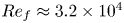 $Re_f \approx 3.2 \times 10^4$) based on the two-dimensional simulations in Härtel et al. (Reference Härtel, Meiburg and Necker2000b). Previously, only the thin layer of ambient fluid below the stagnation streamline close to the bottom in the two-dimensional simulations was deemed to be ingested into the head. In the three-dimensional simulations, the ambient fluid approaching the head may flow directly into the clefts or may be diverted around the lobes and then into the clefts. As can be expected, the fraction of the total flux of ambient fluid ingested in the clefts (
 $Q_1/Q_0$) is apparently greater than the estimates based on previous two-dimensional simulations in the literature.
3.3. Flow field within the head of a gravity current
We have shown in § 3.1 the three-dimensional geometric features of the head of a gravity current. Here, we will examine the flow field within the head of a gravity current in detail. Previous direct numerical simulations have demonstrated that in the lower part of the head of a gravity current, there is a tooth-like vortex inside each lobe. The two legs of the tooth-like vortex have opposite senses of rotation. Along the leading edge of a gravity current, a series of tooth-like vortices align in the spanwise direction, and a pair of counter-rotating vortices are positioned on the left-hand side and right-hand side of each cleft (Espath et al. Reference Espath, Pinto, Laizet and Silvestrini2015; Dai & Huang Reference Dai and Huang2022).
To illustrate the flow field within the head, figure 4 shows the velocity field in the laboratory frame of reference at two horizontal slices for the gravity current propagating on a no-slip boundary at  ${Re=3450}$. The time instance is chosen at
  $t=5.37$ dimensionless units (
 $\tilde {H} \tilde {u}^{-1}_b$). One horizontal slice is taken at
  $x_3=0.05$ (figure 4a) in the lower part of the head, where the lobes and clefts are forming at the leading edge, and the other horizontal slice is taken at
  $x_3=0.33$ (figure 4b) in the upper part of the head, where the steepening bulges are protruding from the upright surface above the clefts. Figure 4(a) shows that in the lower part of the head, the streamwise velocity is higher in the lobes than in the clefts, and the horizontal flow velocity tends to diverge from the lobes and converge to the clefts. Therefore, the streamwise velocity in the lower part of the head may vary within the lobe in the spanwise direction. In the left-hand part of a lobe, the streamwise velocity decreases in the positive spanwise direction, i.e.
  $\partial u_1/\partial x_2 < 0$, and in the right-hand part of a lobe, the streamwise velocity increases in the positive spanwise direction, i.e.
  $\partial u_1/\partial x_2 > 0$. In the lower part of the head, the wall-normal velocity is downwards in the lobes and upwards in the clefts and in the leading edge of the lobes. As we will discuss later, the upward motion in the clefts may not penetrate directly into the upper part of the head, but the upward motion in the leading edge of the lobes may continue to do so in immediate proximity behind the upright surface in the upper part of the head. Figure 4(b) shows that in the upper part of the head, the streamwise velocity is higher away from the upright surface than in immediate proximity behind the upright surface. Detailed inspection indicates that with the presence of the steepening bulges on the upright surface, the streamwise velocity in the upper part of the head may vary in the spanwise direction in the region close to the upright surface. Consequently, in the left-hand part of a steepening bulge, the streamwise velocity decreases in the positive spanwise direction, i.e.
  $\partial u_1/\partial x_2 < 0$, and in the right-hand part of a steepening bulge, the streamwise velocity increases in the positive spanwise direction, i.e.
  $\partial u_1/\partial x_2 > 0$. In the upper part of the head, the wall-normal velocity is downwards away from the upright surface and upward in immediate proximity behind the upright surface. Our findings suggest that while the downward motion of heavy fluid within the head may continue from the upper part of the head to the lobes in the lower part of the head, the upward motion of heavy fluid within the head may also continue from the leading edge of the lobes in the lower part of the head to the region in immediate proximity behind the upright surface in the upper part of the head. The ambient fluid ingested in the clefts tends to rise away from the bottom boundary in the lower part of the head, but the rising ambient fluid may not penetrate directly into the upper part of the head. As we will show later using tracers, the rising ambient fluid is convected towards the leading edge of a gravity current before being carried upwards from the leading edge to the upright surface in the upper part of the head.

Figure 4. Velocity field in the laboratory frame of reference taken at two horizontal slices for the gravity current propagating on a no-slip boundary at  $Re=3450$. The time instance is chosen at
  $t=5.37$ dimensionless units (
 $\tilde {H} \tilde {u}^{-1}_b$), and the two horizontal slices are taken at (a)
  $x_3=0.05$ and (b)
  $x_3=0.33$ to illustrate the flow in the lower part of the head and the flow in the upper part of the head, respectively. The horizontal velocity
  $(u_1,u_2)$ is shown by vectors, and the vertical velocity
  $u_3$ is shown by the thin line contours with solid (dashed) line for positive (negative) vertical velocity. The thick solid lines indicate the location of the front and the location of the upright surface visualized by a density contour
  $\rho =0.1$.
The flow field within the head may be visualized complementarily from a vertical slice within the head of a gravity current. Figure 5 shows the velocity field in the translating coordinate system, and the  $x_1$-component of the vorticity field
 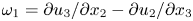 $\omega _1=\partial u_3/\partial x_2-\partial u_2/\partial x_3$ at two vertical slices for the gravity current propagating on a no-slip boundary at
  $Re=3450$. The time instance is chosen at
  $t=5.37$ dimensionless units (
 $\tilde {H} \tilde {u}^{-1}_b$). One vertical slice is taken at
  $x_1=10.21$ (figure 5a), which is at the leading edge of the lobes, and the other vertical slice is taken at
  $x_1=10.04$ (figure 5b), which is at the steepening bulges approximately
  $0.38 d$ behind the leading edge of the gravity current. In the lower part of the head, the flow diverges from the lobe centres and converges to the clefts, and the flow is upwards in the clefts. As shown by figure 5(a), there is a region of positive
  $x_1$ vorticity in the left-hand part of a lobe, and a region of negative
  $x_1$ vorticity in the right-hand part of a lobe, in the range
  $0.03 \lesssim x_3 \lesssim 0.18$. Our results in the lower part of the head are in accord with the findings of tooth-like vortices in Dai & Huang (Reference Dai and Huang2022). Interestingly, as shown by figure 5(b), in the upper part of the head, there is a region of positive
  $x_1$ vorticity in the left-hand part of a steepening bulge, and a region of negative
  $x_1$ vorticity in the right-hand part of a steepening bulge. In the translating coordinate system moving with the head, the streamwise velocity is negative (out of the head) in the region close to the upright surface and in the region close to the bottom boundary, and positive (into the head) in the jets of heavy fluid.

Figure 5. Velocity field in the translating coordinate system and  $x_1$-component of the vorticity field taken at two vertical slices for the gravity current propagating on a no-slip boundary at
  $Re=3450$. The time instance is chosen at
  $t=5.37$ dimensionless units (
 $\tilde {H} \tilde {u}^{-1}_b$). One vertical slice is taken at (a)
  $x_1=10.21$, which is at the leading edge of the lobes, and the other vertical slice is taken at (b)
  $x_1=10.04$, which is at the steepening bulges approximately
  $0.38 d$ behind the leading edge of the gravity current. The velocity
  $(u_2,u_3)$ in the vertical slices is shown by vectors, and the streamwise velocity in the translating coordinate system is shown by the thin line contours with solid (dashed) line for positive (negative) values. The streamwise vorticity field
  $\omega _1$ is visualized by the colour contours. The thick solid lines indicate the surface of the head visualized by a density contour
  $\rho =0.1$.
In order to identify the origin of the streamwise vorticity in the lower and upper parts of the head, we study the  $x_1$-component of the vorticity equation,
 \begin{equation} \frac{{\rm D} \omega_1 }{{\rm D} t} = \underbrace{\omega_1\,\frac{\partial u_1}{\partial x_1}}_{S_1} \underbrace{{}-\frac{\partial u_3}{\partial x_1}\,\frac{\partial u_1}{\partial x_2}}_{S_2} + \underbrace{\frac{\partial u_2}{\partial x_1}\,\frac{\partial u_1}{\partial x_3}}_{S_3} \underbrace{{}-\frac{\partial \rho}{\partial x_2}}_{S_4} + \underbrace{\frac{1}{Re}\,\nabla^2 \omega_1}_{S_5}, \end{equation}
where  $S_1$,
  $S_2$,
  $S_3$,
  $S_4$ and
  $S_5$ represent the stretching of
  $x_1$ vorticity, twisting of
  $x_2$ vorticity, tilting of
  $x_3$ vorticity, baroclinic production of vorticity, and diffusion of
  $x_1$ vorticity, respectively. We should remark that the component
  $(\partial u_1/\partial x_3)(\partial u_1/\partial x_2)$ in the twisting of
  $x_2$ vorticity and the component
  $-(\partial u_1/\partial x_2)(\partial u_1/\partial x_3)$ in the tilting of
  $x_3$ vorticity cancel exactly and have no net effects.
Figure 6 shows the contribution of the twisting of  $x_2$ vorticity, i.e. the
  $S_2$ term, and the contribution of the baroclinic production of vorticity, i.e. the
  $S_4$ term, to the time rate of change of the streamwise vorticity,
  ${\rm D}\omega _1/{\rm D}t$, at two vertical slices for the gravity current propagating on a no-slip boundary at
  $Re=3450$. The time instance is chosen at
  $t=5.37$ dimensionless units (
 $\tilde {H} \tilde {u}^{-1}_b$). Following figure 5, one vertical slice is taken at
  $x_1=10.21$ (figure 6a) at the leading edge of the lobes, and the other vertical slice is taken at
  $x_1=10.04$ (figure 6b) at the steepening bulges approximately
  $0.38 d$ behind the leading edge of the gravity current. The contributions of the stretching of
  $x_1$ vorticity, tilting of
  $x_3$ vorticity and diffusion of
  $x_1$ vorticity, i.e. the
  $S_1$,
  $S_3$ and
  $S_5$ terms, are less than or even of opposite sign to the time rate of change of streamwise vorticity, and are not shown for brevity. From comparison between figures 5 and 6, it is worth noting that both the streamwise vorticity at the leading edge of the lobes in the lower part of the head and the streamwise vorticity at the steepening bulges in the upper part of the head are contributed from the twisting of
  $x_2$ vorticity, i.e. the
  $S_2$ term shown by the colour contours, and the baroclinic production of vorticity, i.e. the
  $S_4$ term shown by the thin solid and dashed lines.

Figure 6. Contribution of the twisting of  $x_2$ vorticity, i.e. the
  $S_2$ term, and the contribution of the baroclinic production of vorticity, i.e. the
  $S_4$ term, to the time rate of change of the streamwise vorticity, i.e.
  ${\rm D}\omega _1 /{\rm D}t$, at two vertical slices for the gravity current propagating on a no-slip boundary at
  $Re=3450$. The time instance is chosen at
  $t=5.37$ dimensionless units (
 $\tilde {H} \tilde {u}^{-1}_b$). One vertical slice is taken at (a)
  $x_1=10.21$, which is at the leading edge of the lobes, and the other vertical slice is taken at (b)
  $x_1=10.04$, which is at the steepening bulges approximately
  $0.38 d$ behind the leading edge of the gravity current. The
  $S_2$ term is visualized by the colour contours, and the
  $S_4$ term is visualized by the thin solid (dashed) lines for positive (negative) contributions. The thick solid lines indicate the surface of the head visualized by a density contour
  $\rho =0.1$.
It is interesting to note that in figure 5(b), the regions of positive and negative streamwise vorticity in the upper and lower parts of the head are positioned at staggered spanwise locations. As we discussed above, the steepening bulges protrude from the upright surface above the clefts, and due to the geometric features of the lobes and the steepening bulges, the streamwise velocity may vary in the spanwise direction. The variation of the streamwise velocity in the spanwise direction results in positive (negative)  $\partial u_1/\partial x_2$ in the right-hand (left-hand) part of a lobe, and positive (negative)
  $\partial u_1/\partial x_2$ in the right-hand (left-hand) part of a steepening bulge. Therefore, the spanwise vorticity is twisted by
  $\partial u_1/\partial x_2$ into the streamwise direction. The contribution of the baroclinic production of vorticity, i.e. the
  $S_4$ term, reinforces the twisting of spanwise vorticity, i.e. the
  $S_2$ term, to the time rate of change of the streamwise vorticity. While the ambient fluid rising from the clefts creates positive (negative) baroclinic production of vorticity in the left-hand (right-hand) part of a lobe, the steepening bulge on the upright surface creates positive (negative) baroclinic production of vorticity in the left-hand (right-hand) part of a steepening bulge on the upright surface.
3.4. Visualization of the flow using tracers
In order to address the questions regarding how the ambient fluid ingested in the clefts ascends within the head of a gravity current, and whether the heavy fluid inside a lobe can be transported to neighbouring lobes in the spanwise direction, we adopt the technique in Dai, Huang & Hsieh (Reference Dai, Huang and Hsieh2021) and Dai et al. (Reference Dai, Huang and Wu2023) to introduce two passive tracers in the simulations in order to track the motion of the ambient fluid ingested in the clefts and the motion of the heavy fluid inside a lobe. The idea of introducing the passive tracers in the simulations is the same as injecting blobs of dye for visualization in the experiments but without intrusively disturbing the propagating gravity current. The passive tracers in the simulations are assumed to have diffusion coefficient  $\tilde {\kappa }$ identical to that of the density field, and in like manner follow the transport equation (2.3).
Figure 7 shows the time evolution of the two tracers implemented in the simulations for the gravity current propagating on a no-slip boundary at  $Re=3450$. The red tracer is used to track the motion of the ambient fluid ingested in and rising from a cleft, and the blue tracer is used to track the motion of the heavy fluid inside a lobe. The initial concentrations for both the red and blue tracers were specified at the time instance
  $t=5.37$ dimensionless units (
 $\tilde {H} \tilde {u}^{-1}_b$). The initial concentration for the red tracer was set at unity in a mushroom-like shape region, where the ambient fluid ingested in the cleft was rising from the bottom boundary, and zero elsewhere. The initial concentration for the blue tracer was set at unity in a rectangular parallelepiped region, where the heavy fluid was inside the lobe, and zero elsewhere. The evolution of the red tracer shows that the ambient fluid ingested in the cleft rises from the bottom boundary and is being swept towards the leading edge of a gravity current. Afterwards, the ambient fluid rising from the cleft is being carried upwards from the leading edge to the upright surface above the left and right neighbouring lobes. The evolution of the blue tracer shows that the heavy fluid inside a lobe may descend while approaching the leading edge of a gravity current. After moving close to the bottom boundary, the heavy fluid inside a lobe may flow forwards towards the leading edge and outwards towards the neighbouring clefts, and ultimately be carried upwards to the upright surface above the left and right neighbouring lobes. Our results indicate that the ambient fluid ingested in a cleft may rise from the bottom boundary to the upright surface through the connection of upward motion between the lower part of the head and the upper part of the head in the leading edge of the lobes, and the heavy fluid inside a lobe may be transported in the streamwise direction and in the spanwise direction across the lobes and clefts.

Figure 7. Time evolution of two passive tracers implemented in the simulations for the gravity current propagating on a no-slip boundary at  $Re=3450$. Time instances are chosen at (a)
  $t=5.37$ , (b)
  $t=5.59$, (c)
  $t=6.22$ and (d)
  $t=7.57$ dimensionless time units (
 $\tilde {H} \tilde {u}^{-1}_b$). The red and blue tracers are used to track the motion of the ambient fluid ingested in a cleft and the motion of the heavy fluid inside a lobe, respectively. The geometry of the head is visualized by a density isosurface
  $\rho =0.1$ with transparent light blue colour. The red and blue tracers are visualized by concentration isosurfaces of
  $0.1$. Spacing between consecutive grid lines in the
  $x_1$ and
  $x_2$ directions is chosen at one-tenth of a dimensionless unit.
4. Conclusions
Gravity currents in the slumping phase from a full-depth lock-exchange configuration with a no-slip boundary are investigated by means of three-dimensional high-resolution simulations of the incompressible Navier–Stokes equations with the Boussinesq approximation. This study complements the findings of tooth-like vortices in Dai & Huang (Reference Dai and Huang2022), and our focus is on the flow within the head of a gravity current propagating on a no-slip boundary.
Our simulations successfully exhibit the geometric features of the head as observed in the laboratory experiments. The geometry of the head is of a three-dimensional nature, which has a series of projecting lobes separated by clefts. Furthermore, the upright surface above the lobes and clefts is corrugated, with steepening bulges protruding from the upright surface above the clefts.
The flow within the head of a gravity current is also of a three-dimensional nature. In the translating coordinate system, the gravity current continuously feeds the head from behind through jets of heavy fluid into the lobe regions. The flux of heavy fluid from the gravity current towards the stationary head ( $Q_2$) is in balance with the flux of heavy fluid carried away by the bottom boundary (
 $Q_3$) and the flux of heavy fluid convected away from the head into the layer above the following current (
 $Q_4$). The ratios
 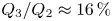 $Q_3/Q_2 \approx 16\,\%$ and
 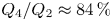 $Q_4/Q_2 \approx 84\,\%$ at Reynolds number
  $Re=17\,000$ (
 $Re_f=3553$) appear to be consistent with the laboratory observations by Simpson & Britter (Reference Simpson and Britter1979). No measurements of the above-mentioned fluxes and ratios have been reported for the head of geophysical gravity currents in the literature. However, Simpson & Britter (Reference Simpson and Britter1979, Reference Simpson and Britter1980) indicate that by comparing with the shape of a dust-laden thunderstorm outflow in Sudan (Lawson Reference Lawson1971) in which the Reynolds number can be estimated to be approximately
  $O(10^8)$, the shape of the gravity current head is essentially independent of the front Reynolds number when
  $Re_f \gtrsim O(10^3)$. Our results of the fluxes and ratios within the head can serve as a reasonable guide for the gravity currents at higher Reynolds numbers, as Simpson & Britter (Reference Simpson and Britter1979, Reference Simpson and Britter1980) alluded to. The fraction of the total flux of ambient fluid ingested in the clefts (
 $Q_1/Q_0$) decreases as the Reynolds number increases, but appears discernibly greater than the corresponding estimates based on the two-dimensional simulations in Härtel et al. (Reference Härtel, Meiburg and Necker2000b). The reason for this discrepancy is that in the three-dimensional simulations, the ambient fluid may flow into the clefts directly or may be diverted around the lobes before entering the clefts, while in the two-dimensional simulations, only a thin layer of ambient fluid below the stagnation streamline close to the bottom boundary was deemed to be entering the head. It should be stressed that although the ratio
  $Q_1/Q_0$ is relatively small, it is essential in the self-sustaining mechanism of the lobe-and-cleft structure, as elucidated by Dai & Huang (Reference Dai and Huang2022), and is nevertheless non-trivial for the geophysical gravity currents at very large Reynolds numbers, e.g. a Sudanese haboob pictured in figure 3.14 of Turner (Reference Turner1979), where the consequent lobe-and-cleft structure is present.
In the lower part of the head of a gravity current, the horizontal velocity diverges from the lobes and converges to the clefts, and the wall-normal velocity is downwards in the lobe regions and upwards in the clefts and in the leading edge of the lobes. In the upper part of the head of a gravity current, the streamwise velocity is higher away from the upright surface, and the wall-normal velocity is downwards away from the upright surface and upwards only in immediate proximity behind the upright surface. Our findings suggest that the downward motion of heavy fluid within the head may continue from the upper part of the head to the lower part of the head in the lobe regions, and the upward motion of heavy fluid within the head may continue from the leading edge of the lobes in the lower part of the head to the region in immediate proximity behind the upright surface in the upper part of the head. Therefore, the lower part of the head and the upper part of the head are interconnected, and the heavy fluid within the head may circulate from the upper part of the head to the lower part of the head in the lobe regions, and ultimately back to the upper part of the head through the leading edge of the lobes. Be mindful that in the two-dimensional model envisioned by Simpson (Reference Simpson1972) and Simpson & Britter (Reference Simpson and Britter1979), the upward circulation in the upper part of the head was thought to be separated from the downward circulation in the lower part of the head by a stagnation streamline, and it was not permissible for the heavy fluid in the upper part of the head to reach the bottom boundary in the lower part of the head. Our results shed a novel light on the understanding of the three-dimensional flow field within the head region.
Based on the results from a vertical slice taken in the spanwise direction within the head, there are regions of positive and negative streamwise vorticity not only in the lower part but also in the upper part of the head. The regions of positive and negative streamwise vorticity in the upper part and in the lower part of the head are positioned at staggered spanwise locations. We have shown that both the streamwise vorticity at the leading edge of the lobes in the lower part of the head and the streamwise vorticity at the steepening bulges in the upper part of the head are contributed from the twisting of spanwise vorticity into the streamwise direction, due to the geometric features of the lobes and the steepening bulges, and contributed from the baroclinic production of vorticity.
Visualization using tracers shows the motion of the ambient fluid ingested in the clefts and the motion of the heavy fluid inside lobes. The ambient fluid ingested in and rising from a cleft is being swept towards the leading edge of a gravity current before being carried upwards from the leading edge to the upright surface above the left and right neighbouring lobes. The heavy fluid inside a lobe may move forwards towards the leading edge and outwards towards the neighbouring clefts, and ultimately be carried upwards to the upright surface above the left and right neighbouring lobes. Our results indicate that the heavy fluid within the head of a gravity current can be transported not only in the streamwise direction but also in the spanwise direction across the lobes and clefts. With the knowledge that the erosive power of a gravity current is concentrated in the head region, it is plausible that the bed material, once resuspended by a gravity current, may be lifted up away from the bottom boundary and be dispersed in both the streamwise and spanwise directions.
The present study complements existing findings in the accompanying paper by Dai & Huang (Reference Dai and Huang2022), and provides new insights into the three-dimensional flow field within the head of a gravity current.
Acknowledgements
A.D. is grateful for encouragement from Professors P. Linden and S. Dalziel at the University of Cambridge, S. Balachandar at the University of Florida, and M. Garcia and G. Parker at the University of Illinois at Urbana-Champaign. Computational resources are provided by the Computer and Information Networking Center at National Taiwan University.
Funding
The research was supported financially by Taiwan National Science and Technology Council through grants NSTC-111-2221-E-002-113-MY3.
Declaration of interests
The authors report no conflict of interest.


 Open access