


1. Introduction
The Deepwater Horizon (DwH) blowout in 2010 resulted in the formation of a long-lived turbulent multiphase plume from the damaged rig site at the ocean bottom. This incident has attracted considerable public and scientific attention. The DwH plume consisted of water containing oil droplets and gas bubbles, and both dispersed phases contributed comparable amounts to the DwH source buoyancy flux with the oil and gas volume flow rate ratio around  $1{:}\,0.8$ (Socolofsky, Adams & Sherwood Reference Socolofsky, Adams and Sherwood2011). The internal dynamics of the DwH plume exhibited multifarious physical, chemical and biological processes, including oil droplet formation, break-up and coalescence, temperature- and pressure-dependent gas dissolution and hydrate formation as well as biodegradation (Socolofsky et al. Reference Socolofsky, Adams, Paris and Yang2016). Additionally, the DwH plume dynamics and the subsequent dispersal of oil both on and below the ocean surface was influenced by external factors such as the ocean density stratification, local currents, waves, winds and the Earth's rotation. This wide range of mechanisms on different length and time scales presents a challenge for modelling the hydrocarbon transport in the environment and for development of effective mitigation strategies.
Motivated by this prominent example of a multiphase plume, we seek to understand the interplay between the background rotation and the additional forcing introduced by the presence of a multiphase effluent in a plume. In this study, we consider a bubble plume released into a rotating unstratified environment and investigate in detail the behaviour of its gas phase. In particular, we focus on the changes of the plume structure caused by the background rotation compared to a multiphase plume in the non-rotating case: we study the rise speed and the lateral spreading of the plume, which are directly related to the subsurface mixing and dispersion of the multiphase effluent and the quantity of gas and oil reaching the surface. Characterising these effects is important for assessing the risks associated with deep-water blowouts and for oil spill mitigation purposes. For example, the correlations for the subsurface location, the amount and the composition of the effluent can be used as the initial conditions for far-field transport models (Socolofsky et al. Reference Socolofsky, Adams, Paris and Yang2016).
Disregarding the wide range of chemical reactions, phase transitions and biochemical processes, the multiphase component can be characterised by the so-called slip velocity  $u_s$, which is the velocity of an individual bubble (or an oil droplet) relative to the surrounding fluid and can lead to the separation between the gas bubbles (or oil droplets) and the entrained water plume. Asaeda & Imberger (Reference Asaeda and Imberger1993) and Socolofsky & Adams (Reference Socolofsky and Adams2005) investigated in laboratory experiments the effects of the slip velocity
  $u_s$ on the bubble plume structure and the formation of subsurface lateral intrusions in quiescent non-rotating stratified environments. Depending on the relative magnitude of the slip velocity
  $u_s$ to the characteristic plume velocity
  $(BN)^{1/4}$ in a stratified environment, where
  $B$ is the source buoyancy flux and
  $N$ is the buoyancy frequency of the stratification, three plume types can be identified that differ in the pattern of the lateral detrainment and the structure of secondary plumes. In the DwH case, it is estimated that bubbles rise faster than oil droplets so that
  $u_s$ can be based on the effective gas droplet diameter (Socolofsky et al. Reference Socolofsky, Adams and Sherwood2011). The non-dimensionalised slip velocity
  $u_{Ns}=u_s/(BN)^{1/4}$ can therefore be placed in the range between
  $0.6$ and
  $1.5$ (Fabregat Tomàs et al. Reference Fabregat Tomàs, Poje, Ozgokmen and Dewar2017; Socolofsky et al. Reference Socolofsky, Adams and Sherwood2011) which, following the classification by Socolofsky & Adams (Reference Socolofsky and Adams2005), renders the DwH plume a Type 1* plume with a single distinct subsurface intrusion layer. Understanding the effects of
  $u_N$ on the plume structure is therefore crucial for modelling the vertical and horizontal transport of oil and gas after deep-water blowouts.
The duration of the DwH spill of several months implies that the DwH plume is likely to have been affected by the Earth's rotation with angular velocity  $\varOmega _E$. The conventionally defined Rossby number
  $Ro_s=N/f$ for the DwH plume is moderate
  $Ro_s\approx 10$, where
  $f=2\varOmega _E\sin \theta$ is the vertical component of the Coriolis frequency at latitude
  $\theta .$ However, previous numerical and experimental studies showed that even at such moderate Rossby numbers, we can expect the background rotation to alter significantly the plume dynamics if the plume is maintained for a sufficiently long time (Fabregat Tomàs et al. Reference Fabregat Tomàs, Poje, Ozgokmen and Dewar2016; Frank et al. Reference Frank, Landel, Dalziel and Linden2017). In particular, regardless of the Rossby number, the system rotation modifies the plume dynamics after one rotation period due to the conservation of the angular momentum (Frank et al. Reference Frank, Landel, Dalziel and Linden2017). The DwH oil spill occurred at the latitude of
  $\theta \approx 28.7^{\circ }$ at which the Earth's rotation period is approximately
  $T=50\ \textrm {h}\approx 2\ \textrm {d}$. During the spill duration of 87 days, the DwH oil plume is hence very likely to have been significantly impacted by the Earth's rotation with associated substantial changes in the plume dynamics.
Laboratory studies of single-phase plumes in a homogeneous rotating environment were conducted by Fernando, Chen & Ayotte (Reference Fernando, Chen and Ayotte1998) and Goodman et al. (Reference Goodman, Collins, Marshall and Pierrhumbert2004). Fernando et al. (Reference Fernando, Chen and Ayotte1998) proposed expressions for the critical times when the plume rise height and width start to be affected by the background rotation:  $\varOmega t\approx 2.4$ and
  $\varOmega t\approx 5.5$, respectively, where
  $\varOmega$ is the rotation rate of the environment and
  $t$ is the time. Sheremet (Reference Sheremet2004) studied the scenario when there is a finite angle between the direction of gravity and the vector of rotation and documented novel features in the plume development that are absent in the case of no misalignment, such as, for example, the plume flow direction being intermediate between the gravity acceleration and rotation vectors, as well as the formation of tilted plume structures. Helfrich & Battisti (Reference Helfrich and Battisti1991) investigated the development of a single-phase plume from a point source in a stratified rotating environment and established that a cyclonic circulation forms in the vicinity of the source and an anticyclonic eddy at the height of the lateral intrusion (that exists provided that the ambient fluid is deep enough, i.e.
  $H\gtrsim 5(BN^{-3})^{1/4}$). Furthermore, they observed that the thickness of the intrusion layer grows with decreasing Rossby number and the plume acquires a cylindrical shape. Convection from extended sources in a homogeneous rotating environment was examined by Maxworthy & Narimousa (Reference Maxworthy and Narimousa1994). They noted that beyond a critical vertical distance from the source,
  $z\approx 12.7(B_a /f^{3})^{1/2}$ with
  $B_a$ being the buoyancy flux per unit area, the advancing three-dimensional turbulent front disintegrates by dividing into a field of columnar vortices with a characteristic diameter
  $\sim (B_a/ f^{3})^{1/2}$ and vertical propagation speed
  $\sim (B_a/ f)^{1/2}$. The vortex generation from buoyant line sources was investigated in detail by Bush & Woods (Reference Bush and Woods1999) for both stratified and homogeneous rotating environments. In particular, in a homogeneous case if the line plume is affected by the background rotation before it impinges on the free water surface, Bush & Woods (Reference Bush and Woods1999) reported the formation of unsteady anticyclonic columns of characteristic radius
  $\sim B_l^{1/3}/f$ with
  $B_l$ the source buoyancy flux per unit length. Possibly most relevant to the current study, Frank et al. (Reference Frank, Landel, Dalziel and Linden2017) observed and characterised the anticyclonic precession of the plume axis for a single-phase plume from a point source in a homogeneous rotating environment: the plume exhibits a pronounced lateral tilt after approximately one rotation period and the precession frequency
  $\omega$ depends linearly on the background rotation speed as
  $\omega \approx (0.4\pm 0.04)\varOmega$. The phenomenon of the anticyclonic plume precession was also observed in experiments by Ma, Flynn & Sutherland (Reference Ma, Flynn and Sutherland2019) who confirmed the linear relationship between the precession frequency and the background rotation, although they reported a slightly higher proportionality factor
  $\omega \approx (0.52\pm 0.09)\varOmega$.
These previous studies examine the effects of rotation on the dynamics of single-phase plumes and provide useful background for the present investigation. However, at the time of writing, there appears to be no experimental studies that additionally consider the presence of a multiphase plume in a rotating environment. A recent numerical simulation of bubble plumes in a rotating environment was conducted by Fabregat Tomàs et al. (Reference Fabregat Tomàs, Poje, Ozgokmen and Dewar2017). Using a simple Eulerian–Eulerian Boussinesq model for the monodisperse gas phase, where the gas phase is treated as a Eulerian scalar field obeying a convection–diffusion equation and is characterised by a slip velocity  $u_s$, they studied the behaviour of a bubble plume at Rossby numbers and slip velocities comparable to the estimates for the DwH oil plume. Such an approach does not model directly the bubble-induced turbulence, but Fabregat Tomàs et al. (Reference Fabregat Tomàs, Poje, Ozgokmen and Dewar2017) stated that the simple slip velocity formulation sufficiently captures the increase in turbulence production observed in the presence of bubbles. The simulations were conducted for a stratified rotating environment and represented direct numerical simulations of the plume at laboratory scale at a Reynolds number of 7000 based on the characteristic plume velocity and length scales,
  $(BN)^{1/4}$ and
  $(BN^{-3})^{1/4}$, respectively. The main finding of these simulations was that the presence of the gas phase amplifies the rotational effects and also changes the plume structure and dispersion compared to a single-phase plume in a rotating environment. In particular, compared to single-phase plumes, the presence of the gas phase leads to a greater decrease of the detrainment height, a thickening of the intrusion layer, and it elevates the near-source concentration of a passive tracer injected at the source of the buoyant plume.
The goal of the present study is to investigate experimentally the dynamics of a multiphase turbulent plume from a point source in a homogeneous environment under the combined effects of the background rotation and the presence of a buoyant gas phase. We generated several bubble size distributions and characterised them by the slip velocity  $u_s$ of the bubble species that contributed most to the buoyancy flux. For the non-rotating homogeneous environment, a characteristic plume velocity scale is given by
  $(B/H)^{1/3}$ (Morton, Taylor & Turner Reference Morton, Taylor and Turner1956), where
  $B$ is the plume buoyancy flux and
  $H$ is the water depth, so that a non-dimensionalised slip velocity can be defined as
  $u_N=u_s/(B/H)^{1/3}$. Note that
  $u_N$ is related to the dimensionless parameter
  $M_H=B/(4{\rm \pi} \alpha ^{2}Hu_s^{3})$ used by Asaeda & Imberger (Reference Asaeda and Imberger1993) as
  $u_N=(4{\rm \pi} \alpha ^{2} M_H)^{-1/3}$, where
  $\alpha$ is the entrainment coefficient. Since
  $M_H=D/H$, where
  $D$ is the length scale defined by Bombardelli et al. (Reference Bombardelli, Buscaglia, Rehmann, Rincón and García2007),
  $u_N$ can be expressed as
  $u_N=(4{\rm \pi} \alpha ^{2}D/H)^{-1/3}$. In the experiments reported in this paper,
  $u_N$ ranges between
  $0.06$ and
  $0.36$. We also vary the Rossby number
  $Ro=(B\varOmega ^{-3})^{1/4}/H$ in the range
  $0.03\lessapprox Ro \lessapprox 0.3$ by changing the buoyancy flux
  $B$ and the system rotation rate
  $\varOmega$. We note that, in this study, the plume buoyancy flux
  $B$ is solely due to the presence of bubbles released at the plume source, and we focus only on characterising the gas phase and do not analyse the liquid phase of the plume.
The present work aims to fill the gap left by the scarcity of experimental results on multiphase plumes in a rotating environment. Although stratification was a very important factor for the dynamics of the DwH plume, we consider here the simplified problem of a multiphase plume released into a homogeneous rotating environment. The present investigation is intended as a first step in the study of the largely unexplored research area on multiphase plumes in a rotating environment. We intend to include stratification in future experiments. We focus here on three particular aspects of the problem. First, we consider the initial rise characteristics of the bubble plume, such as the rise height and the lateral spreading of the gas phase, and how they depend on the interplay between the slip velocity and the rotation of the environment. Second, we briefly discuss the subsurface bubble distribution after the plume has risen through the entire water column and has reached the free surface. Last, as an externally accessible diagnostic, we consider the signature of the bubble plume at the free surface and how it evolves in time.
The paper is structured as follows. We describe our experimental set-up and the experimental procedure in § 2.1. The bubble source conditions (the buoyancy flux  $B$ and the bubble size distributions) are characterised in § 2.2. Section 2.3 explains our procedure for the data analysis. Section 3 presents our experimental results with § 3.1 briefly focusing on bubble plumes in a non-rotating environment before considering features specific to rotating plumes. Sections 3.2, 3.3, 3.4 and 3.5 explore the anticyclonic plume precession, the initial rise characteristics, the late-stage evolution and the surface footprint of the plume, respectively. The findings of this paper are summarised in § 4, where we also briefly discuss the relevance of our results for geophysical plumes and deep-water oil plumes such as the 2010 DwH oil spill plume.
2. Experiments
2.1. Experimental set-up
We conducted 144 experiments on bubble plumes discharged at the base of a homogeneous rotating saltwater environment. A schematic of the experimental set-up is shown in figure 1. The experimental tank, located on a rotating table and described in detail in Frank et al. (Reference Frank, Landel, Dalziel and Linden2017), had an octagonal base with a circumscribed circle diameter of 1 m and a maximum depth of 1.2 m. The rotation rate  $\varOmega$ used was typically varied in the range
  $0\text {--}1\ \textrm {rad}\ \textrm {s}^{-1}$, with an incremental step of
  $0.1\ \textrm {rad}\ \textrm {s}^{-1}$. Typically, the tank was filled to a depth of
  $H=0.6\ \textrm {m}$.

Figure 1. (a) Schematic of the experimental set-up, (b) photograph of the experimental tank and (c) schematic and photograph of the bubble source generator.
The bubbles were produced by means of electrolysis. The bubble source generator, manufactured in house, consisted of a tube, with a 15 mm inner diameter and a 50 mm length, which was connected to a circular plastic base (figure 1c). Six layers of electrodes, each comprising multiple  $127\ {\rm \mu}{\rm m}$ diameter platinum wires arranged in a semi-random manner, spanned the generator tube at different heights. These electrodes were connected to the power supply such that there were three layers of cathodes alternating with three layers of anodes so that both hydrogen and chlorine gas bubbles were produced. Small holes were cut through the tube wall next to where it connected to the plastic base to form a chimney that emits a two-phase flow of saltwater and bubbles. The bubble generator was hidden underneath a false bottom in the tank except for the top approximately 30 mm, which protruded through a 40 mm diameter hole in the centre of the false bottom.
The bubble generator was connected to a computer-controlled power supply. The number and the size of the bubbles produced depended on the current  $I$ flowing through the bubble source and the salt concentration (and hence the density
  $\rho _a$) of the ambient saltwater. For our experiments, we used two different saltwater densities
  $\rho _a\approx 1008\ {\rm kg}\ {\rm m}^{-3}$ and
  $1179\ \textrm {kg}\ \textrm {m}^{-3}$ and four different currents
  $I=0.3$, 0.5, 0.7, 0.9 A. Table 1 summarises our experimental parameters. Note that the gas production rate
  $Q$ used to calculate the source buoyancy flux
  $B$ was measured by collecting the gas bubbles in a measuring cylinder that was initially filled with water. This is explained in detail in § 2.2 and appendix A.
Table 1. Overview of the parameters used in our experiments.

The flow was recorded using two JAI Spark SP-5000C-CXP2 5-megapixel cameras that were fixed in the rotating frame of reference: one camera was attached to the sidewall of the tank and the other recorded the top view (figure 1a,b). We used the side illumination by means of two red LED panels for the side-view recordings of the plume. For the top-view recordings, a 2 mm thick horizontal laser sheet created by a 32 mW 520 nm Flexpoint laser, fitted with a 45 $^{\circ }$ Powell lens, was positioned approximately 15 mm below the water surface. The centrifugal force, caused by the rotation of the tank, produced a curvature of the water surface, especially for high values of
  $\varOmega$, so that the water level was depressed at the tank centre. As a consequence, the laser sheet was closer to the water surface in the centre of the tank than at the tank edges. Unfortunately, no simultaneous side-view and top-view recordings could be made because the light from the side LED panels would have interfered with the laser sheet and polluted the top-view videos. Instead, each experiment was repeated for the same experimental conditions twice: once recording with the side-view camera, and once with the top-view camera. The side-view camera was equipped with a wide angle 6 mm c-mount lens that allowed visualisation of the entire vertical extent of the plume from the source to the free surface.
The experimental procedure was as follows. The tank was spun up from rest for at least eight spin-up times  $T_s=H(\nu \varOmega )^{-1/2}/4$ (Greenspan & Howard Reference Greenspan and Howard1963), where
  $\nu$ is the kinematic viscosity of water, until it reached solid body rotation. The video recording was started and, immediately, the bubble source was switched on with the selected current. The plume was captured for 300 s at 10 frames per second for the side-view and at 5 frames per second for the top-view videos. The exposure time was set to 100 and 200 ms, respectively. We note that for the source buoyancy fluxes
  $B$ used, the rising times of the plume through the water column were of the order of magnitude of 20 s. Furthermore, the fixed recording time of 300 s corresponded to approximately
  $5$ rotation periods for
  $\varOmega =0.1\ \textrm {rad}\ \textrm {s}^{-1}$ and
  $50$ rotation periods for
  $\varOmega =1\ \textrm {rad}\ \textrm {s}^{-1}$. In practice, we used only the first 120 s of our recordings for the data analysis. At the end of an experiment, the bubble source was switched off and a new rotation rate for the tank was selected. After an appropriate amount of time that was sufficient for the remaining bubbles to disappear and for the water in the tank to equilibrate in a new solid body rotation state, a minimum of four spin-up times
  $T_s$, a new experiment could be started. We changed the water in the tank approximately every 10 experiments to avoid any yellow colouring of the water in the tank caused by potential secondary chemical reactions of other impurities. No evidence of a significant gas dissolution in the plume was observed during an experimental run.
2.2. Measuring the source buoyancy flux and the bubble size distribution
In order to characterise the bubble plumes, we needed to determine both the source buoyancy flux  $B$ (which is governed by the current
  $I$ through the bubble generator) and the size distribution of the bubbles produced in order to estimate the bubble slip velocity
  $u_s$. The methods used to measure
  $B$ and
  $u_s$ are described in detail in appendices A and B, respectively.
The gas production rate  $Q$ was found not to depend significantly on the salinity of the ambient water and to scale approximately linearly with the source current
  $I$. The source buoyancy flux
  $B$ is inferred from the gas production rate
  $Q$ as
 \begin{equation} B=gQ, \end{equation}
where  $g=9.81\ \textrm {m}\ \textrm {s}^{-2}$ is the acceleration due to gravity. Table 1 includes the approximate source buoyancy fluxes
  $B$ that were achieved for each experiment.
The bubble size distribution of the bubble generator was measured using a procedure described in detail in appendix B. The probability distribution of the bubble radii  $r$ is reasonably well approximated by a log–normal distribution
  $f_r(r)$, i.e.
  $\ln f_r(r)\sim \mathcal {N}(\mu ,\sigma )$, where
  $N(\mu ,\sigma )$ is a normal distribution with the mean value
  $\mu$ and the standard deviation
  $\sigma$. Table 2 lists the values of the associated parameters
  $\mu$ and
  $\sigma$ for the fitted log–normal distributions. The radius corresponding to the peak of each distribution, denoted by
  $r_{m}$, is calculated as
  $\exp (\mu -\sigma ^{2})$.
Table 2. Parameters and measured values for the bubble size and buoyancy distributions.

The buoyancy distribution function  $f_b(r)$ is calculated from the bubble radius distribution function
  $f_r(r)$ by multiplying the latter by
  $r^{3}$ and normalising it
 \begin{equation} f_b(r)=\frac{r^{3} f_r(r)}{\displaystyle\int_0^{\infty} r^{3} f_r(r)\,{\textrm{d}}r}. \end{equation}
The bubble radii corresponding to the peaks of the buoyancy distribution functions are labelled as  $r_{mb}$ and their values are recorded in table 2.
We characterise each bubble size distribution by the slip velocity  $u_s$ based on the bubble radius
  $r_{mb}$ containing the largest contribution to the buoyancy flux. The slip velocity
  $u_s$ is calculated from the balance of the buoyancy force and the friction force acting on a bubble (Stokes’ law)
 \begin{equation} \tfrac{4}{3}{\rm \pi} r_{mb}^{3} g \rho_a=6{\rm \pi}\mu_{dyn}r_{mb}u_s, \end{equation}
where  $\mu _{dyn}$ is the dynamic viscosity of saltwater. Table 2 includes the values calculated for
  $u_s$ and also for the non-dimensionalised bubble slip velocity
  $u_N$. Note that the Reynolds number
  $\textit {Re}_b$ based on the bubble radius of 50 mm, the slip velocity of 0.5 cm s
 $^{-1}$ and the kinematic viscosity of water of
  $10^{-6}\ \textrm {m}^{2}\ \textrm {s}^{-1}$ can be estimated as
  $\textit {Re}_b\approx 0.25$ which means that the flow around the bubble is laminar and (2.3) applies.
2.3. Image analysis
We analyse the experimental data by means of a formalised automated procedure for the post-processing of image sequences. In the following, we present this algorithm and, in particular, discuss our definition of the plume extent.
The recorded side-view raw image sequence shows the plume as a bright structure against a black background. The bubbles reflect the light from the side LED panels into the camera: the more bubbles that are present at a certain location (integrated in the direction normal to the camera field of view), the greater the light intensity and the brighter this location appears in an image. Appendix C shows an example of the experimental images of the plume at each stage of the post-processing. The camera recorded the raw images in the 8-bit system. We note that in the 8-bit system where ‘black’ is 0 and ‘white’ is 255, a typical mean light intensity of the raw background image in our experiments was around 9.5. A typical temporal variation in the light intensity of a background pixel (that was not affected by the plume at any time) was at most 1 or 2 in the 8-bit system. The first image of a recorded sequence, when the plume is not yet started, is used to remove the background from the subsequent frames through a simple transformation: the photographic negative (i.e. the image, normalised by the saturated intensity of 255, then subtracted from one) of every frame in the sequence is divided by the photographic negative of the first frame
 \begin{equation} \hat{\mathcal{I}} =\frac{1-\mathcal{I}}{1-\mathcal{I}_0}.\end{equation}
Here,  $\mathcal {I}$ is the raw intensity of the image,
  $\mathcal {I}_0$ is the intensity of the first frame and
  $\hat {\mathcal {I}}$ is the intensity of the transformed image. This yields a sequence of images where the plume now appears as a dark structure against a white background. Upon a close inspection of these new transformed images, we found that the white background possesses a very uniform intensity
  $\hat {\mathcal {I}}$. The light intensity
  $\hat {\mathcal {I}}$ of most background pixels assumes values in the range of
  $0.996{-}1$ where ‘white’ is considered as 1 and ‘black’ as 0. Thus, we convert these transformed images into binary images of the plume where every pixel with the light intensity
  $\hat {\mathcal {I}}<0.995$ is considered to contain bubbles.
We now formalise our definition of the plume extent: the plume is defined to be the largest connected object in a binary image – effectively, the two-dimensional projection or silhouette of the plume. At each time step, the search for the largest object with pixels connected by any one of their eight nearest neighbours is performed using MATLAB® 2016a.
Our choice of the plume as the largest connected object ensures that individual large bubbles that escape due to their slip velocity are not considered to be a part of the plume. In other words, a region is within the plume if the number of bubbles in this region is high enough and there is a gapless path between the imaged pixel of this region and the plume source. We note that the light intensity in our images is integrated in the direction normal to the camera field of view, so ‘a region’ is a two-dimensional projection of a three-dimensional object. In practice, this may lead to some uncertainty around the boundary where an edge region may or may not be considered to be a part of the plume depending on the orientation of the projection. However, this higher-order distinction would require either information of both gas and liquid-phase velocity field or a complete three-dimensional mapping of the plume structure.
Our definition of the plume extent is based on the distribution of the bubbles alone, since the light intensity distribution is linked to the bubble distribution, rather than on the liquid-phase velocity field. It accounts only for the presence of the bubble phase and not for the liquid phase since no information on the latter can be extracted from our experimental data. Under field conditions in real oceans, our definition of the plume extent would correspond to using a probe that measures the chemical composition of water and determines the pollutant concentration (for example, oil or gas). Then we define a location  $\boldsymbol x$ to be within the plume if the pollutant concentration (accumulated along a horizontal line with a chosen direction through
  $\boldsymbol x$) surpasses a certain threshold and there is a gapless path within the plume from
  $\boldsymbol x$ to the plume source. If the concentration accumulated along a horizontal line through
  $\boldsymbol x$ is too low – too little light is scattered into the camera in our experiments – then
  $\boldsymbol x$ is not regarded as being part of the plume. This definition is sensible because first, we have a direct access only to the light intensity field and not to the velocity field. Second, the radial profile of the vertical velocity for a plume in a rotating environment is no longer expected to follow a well-defined Gaussian distribution at each height, but exhibits a rather complicated structure with the flow reversal around the plume edges (see further discussion in § 3.3.3 and Fernando et al. Reference Fernando, Chen and Ayotte1998). Furthermore, we do not expect any azimuthal bias based on the view point of the camera, owing to the axisymmetric geometry of the set-up and the turbulent nature of the plume flow. Thus, our plume definition shows representative behaviours, especially when experiments are regarded in their ensemble.
The binary images are subsequently used for determining the edges of the plume in MATLAB® 2016a. The detected edges are stored in a three-dimensional array with two spatial and one time dimension. In each pixel row of the image, the leftmost pixel where an edge has been detected is considered to be the left bounding edge of the plume and the rightmost edge pixel is defined as the right bounding edge of the plume. The region between the left and the right bounding edges is now defined as the extent of the plume and at each height, the width of the plume  $b$ is the distance between the left and the right bounding edge.
A similar procedure is used in the post-processing of the top-view images.
3. Results
3.1. Bubble plume in a non-rotating environment
Before investigating the combined effects of the bubble slip velocity and the ambient rotation rate on the plume dynamics, we briefly discuss the role of the bubble slip velocity for the plume in a non-rotating environment. McDougall (Reference McDougall1978) modelled a bubble plume as consisting of an inner core in which the majority of the bubbles are concentrated and which is surrounded by an annular flow of the entrained fluid. Milgram (Reference Milgram1983) described the bubble plume as a single plume of bubbles and water with different Gaussian profiles for the velocity and density defect which were based on the plume radius and the smaller gas-containing radius, respectively. We reiterate that our imaging technique only captures the gas phase. Thus, hereafter ‘the plume’ only refers to the gas phase.
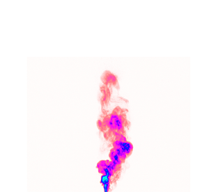
Figure 2 shows average images of the plume for  $B=50\ \textrm {cm}^{4}\ \textrm {s}^{-3}$ for two values of the non-dimensionalised slip velocity
  $u_N = 0.07$ and 0.27. The averaging was performed over 60 s (600 frames) after the plume has reached the free water surface. The conical shape of the plume (bubble phase) appears visually thinner for a larger slip velocity
  $u_N$ (which corresponds to a smaller ambient density
  $\rho _a$, see table 2). We formalise this by considering the vertical region between
  $10d_0$ and
  $25d_0$ above the nozzle (indicated by vertical double arrows in figure 2), where
  $d_0$ denotes the inner diameter of the bubble source. In each pixel row, a Gaussian is fitted to the light intensity distribution using a least-squares procedure. The standard deviations
  $\sigma _b$ of the fitted Gaussians as a function of height
  $z$ above the nozzle are displayed in figure 3 for different
  $u_N$. We observe that
  $\sigma _b\sim z$ so that a linear fit
  $\sigma _b=\alpha _b z$ can be made: the coefficient
  $\alpha _b$ as a function of
  $u_N$ is shown as the inset in figure 3 with the red dashed line showing the value for the entrainment constant
  $\alpha =0.12$ of a single-phase plume (see e.g. Morton et al. Reference Morton, Taylor and Turner1956; Papanicolaou & List Reference Papanicolaou and List1988). This confirms our qualitative observation that the plume width reduces with increasing
  $u_N$. We note that the coefficient
  $\alpha _b$ cannot be regarded as the entrainment constant of the plume since the entrainment is defined for the liquid phase which we do not visualise.

Figure 2. Average images of the plume for 60 s (600 frames) after the plume has reached the free water surface for  $B=50\ \textrm {cm}^{4}\ \textrm {s}^{-3}$ and for (a)
  $u_N=0.07$ (series B) and (b)
  $u_N=0.27$ (series F). The plume shape appears thinner for a larger non-dimensional bubble slip velocity. The vertical double arrows indicate the range of heights at which Gaussian curves were fitted to the light intensity distribution. Blue dashed lines show the linear fits
  $\alpha _b z$.

Figure 3. The non-dimensional standard deviation  $\sigma _b/d_0$ of the Gaussian curves fitted to the light intensity
  $x$-distribution of average plume images (see figure 2) as a function of the non-dimensional height
  $z/d_0$ above the nozzle, and the non-dimensional slip velocity
  $u_N$ (colours). See table 2 for the experimental parameters. The inset figure shows the coefficient
  $\alpha _b$ of the linear least-square fits to
  $\sigma _b/d_0$ curves as a function of
  $u_N$. The red dashed line shows the value for the entrainment constant
  $\alpha =0.12$ of a single-phase plume.
The next feature we investigate is the effect of the bubble slip velocity on the initial rise height of the plume. For a single-phase plume from a point source with a source buoyancy flux  $B$ in a homogeneous non-rotating environment, the rise height
  $h$ of the plume front is expected to scale as
 \begin{equation} h \sim B^{1/4} t^{3/4}, \end{equation}
where  $t$ is the time after the start of the plume (Turner Reference Turner1962).
The rise height  $h$ of the plume at each time point is calculated as the distance from the source to the lowest height near the top of the plume where the width of the plume first vanishes (based on the criterion described in § 2.3). Figure 4 shows a log–log plot of
  $h/H$ as a function of the non-dimensionalised time
  $(B/H^{4})^{1/3} t$. We set
  $t=0$ as the time when the plume starts. With the gas phase present, the height of the plume grows slightly faster than the scaling
  $t^{3/4}$ for homogeneous plumes. We fit the rise height
  $h$ with a power law of the form
  $at^{\beta }$ up to the height of
  $25d_0$ and find that the power coefficient
  $\beta$ varies between approximately
  ${\sim }t^{0.75}$ and
  ${\sim }t^{0.87}$. Based on the entire set of data presented in this paper and by considering the repeatability of experiments (see also § 3.3.1 and, in particular, figure 6), the error associated with the power coefficients is estimated to be
  ${\pm }0.03$. Thus, an increase in the power-law coefficient with an increasing
  $u_N$ is statistically significant. Here, we stress that we define the plume rise height as the vertical extent of the largest connected structure in the bubble plume, as determined by our criterion described in § 2.3. For the series E, F, G and H, we observed that some individual bubbles separated from the plume front and rose faster than the plume. Had the height of the plume been based on the rise height of these separated bubbles, then the scaling would follow approximately
  $h/H\sim t$, a speed comparable with that of the individual bubbles in isolation.

Figure 4. The non-dimensionalised rise height  $h/H$ of the plume front in a non-rotating environment as a function of the non-dimensionalised time
  $(B/H^{4})^{1/3} t$, where
  $H$ is the water depth above the source, for different
  $u_N$. With gas bubbles present, the exponent
  $\beta$ is slightly larger than
  $3/4$ and rises to approximately
  $0.87$. The inset figure shows the exponent
  $\beta$ of the power-law fit to the rise height
  $h$ as a function of
  $u_N$.
We can attribute the value of  $\beta$ being larger than
  $3/4$ to the bubble slip velocity and our definition of the plume. Specifically, we consider only the bubble phase of the plume and define a region to be within the plume if the concentration of bubbles in that region is high enough. It would be interesting to see what happens to the liquid phase upon starting the bubble plume and what power law the rising plume front follows if it is defined by means of a passive (dye) tracer injected at the source. Predicting the value of
  $\beta$ and how it depends on
  $u_N$ would be valuable in order to understand better the impact of bubbles on the plume dynamics. Likewise, investigating further the dependence of
  $\alpha _b$ on
  $u_N$ would be useful for understanding the dynamics of these multiphase plumes. A careful study of these problems, however, would require a larger data set for a wider range of slip velocities than we currently have. This would also require measurements of the velocity field of the liquid phase of these plumes. The data presented in this section are primarily included as a base non-rotating case (
 $\varOmega =0\ \textrm {rad}\ \textrm {s}^{-1}$) to allow for comparison between the rotating and the non-rotating cases and for determining the effects of background rotation discussed in the following sections.
3.2. Precession frequency of the bubble plumes in a rotating environment
The bubble plumes exhibited essentially the same lateral deflection and precession phenomenon that was reported in Frank et al. (Reference Frank, Landel, Dalziel and Linden2017) for single-phase plumes: after approximately one rotation period, the plume was deflected laterally and then started to precess in the anticyclonic direction. When viewed from above, the tank was rotating in the counter-clockwise direction, so the direction of the observed precession was clockwise relative to the tank. We use a similar procedure to that of Frank et al. (Reference Frank, Landel, Dalziel and Linden2017), based on the Hilbert–Huang transform, to extract the precession rate of the plume axis. Figure 5 shows the extracted mean precession rate  $\bar \omega$ of the bubble plume as a function of
  $\varOmega$. We observe that
  $\bar \omega$ is a linear function of
  $\varOmega$ with a proportionality factor
  $0.41\pm 0.05$, which is a similar value to single-phase plumes (
 $\omega \approx (0.4\pm 0.04)\varOmega$, Frank et al. (Reference Frank, Landel, Dalziel and Linden2017) and
  $\omega \approx (0.52\pm 0.09)\varOmega$, Ma et al. Reference Ma, Flynn and Sutherland2019). The error estimate for the proportionality factor is based on the
  $95\,\%$ confidence interval for the coefficient estimate of the linear regression model. The independence of
  $\bar \omega$ from
  $B$ was already shown experimentally in the previous study (Frank et al. Reference Frank, Landel, Dalziel and Linden2017). Here, we confirm that the precession rate is also independent of the bubble slip velocity
  $u_N$. This is to be expected from the theoretical spinning-top toy model developed by Frank et al. (Reference Frank, Landel, Dalziel and Linden2017). The theoretical estimate (see (5) in that study) for the precession frequency
  $\bar \omega$ relies on the value for the entrainment coefficient as one of the main factors. Bubble plumes considered in this paper may be less turbulent at the source and lazier, and possess an entrainment coefficient smaller than 0.1. However, changing the value of the entrainment coefficient to 0.08 instead of 0.1 used in Frank et al. (Reference Frank, Landel, Dalziel and Linden2017) results only in a marginally different proportionality factor of 0.43 instead of 0.35, that would be expected from the theoretical estimate. Such a difference is unlikely to be observed experimentally in the proportionality factor for the precession frequency, especially when taking into consideration the scatter of the data presented in figure 5.

Figure 5. Extracted precession rate  $\bar \omega$ of bubble plumes as a function of the rotation rate
  $\varOmega$ for different source buoyancy fluxes
  $B$ and slip velocities
  $u_N$. The precession rate
  $\bar \omega$ scales linearly with
  $\varOmega$, with a proportionality factor of
  $0.41\pm 0.05$, similar to single-phase plumes, and appears to be independent of
  $u_N$.
3.3. Initial rise of the bubble plume in a rotating environment
In this section we investigate the combined effects of the slip velocity  $u_N$ and the rotation rate
  $\varOmega$ on the initial rise characteristics of the bubble plume, before the plume reaches the free water surface. For deep-water blowouts, or naturally occurring oceanic plumes in general, the only information readily available are the ocean surface observations. Therefore, here we first investigate the time delay between the initiating of the plume at the bottom and the appearance of its signature on the water surface. We also discuss the distribution of the plume fluid inside the water column by considering the rise height of the plume silhouette centroid and the disintegration of the first plume front.
3.3.1. Rise height of the plume front
The rise height  $h$ of the plume, determined as described in § 3.1, is plotted in figure 6 for six experimental series (see table 1) with
  $t=0$ and
  $h=0$ defined as before. We non-dimensionalise
  $h$ as
  $h/(B\varOmega ^{-3})^{1/4}$ and the time
  $t$ as
  $\varOmega t$, similarly to the scalings introduced by Fernando et al. (Reference Fernando, Chen and Ayotte1998). For
  $\varOmega t \to 0$, we expect
 \begin{equation} \frac{h}{(B\varOmega^{{-}3})^{1/4}}\sim (\varOmega t)^{3/4},\end{equation}
which coincides with (3.1) for the rise height of a single-phase plume in a non-rotating environment. Fernando et al. (Reference Fernando, Chen and Ayotte1998) found that the rise height of the plume slows down from the  $3/4$ power law for
  $\varOmega t \gtrsim 2.4$.

Figure 6. Double-logarithmic plot of the non-dimensionalised rise height  $h/(B\varOmega ^{-3})^{1/4}$ as a function of the non-dimensionalised time
  $\varOmega t$ for six experimental series. The experimental parameters are listed in table 1. (a) Series A,
  $u_N=0.06$; (b) series C,
  $u_N=0.08$; (c) series E,
  $u_N=0.23$; (d) series F,
  $u_N=0.27$; (e) series G,
  $u_N=0.31$; and (f) series H,
  $u_N=0.36$.
Close inspection of the rise height of bubble plumes presented in figure 6 does not reveal any observable change in the ascent of the plume front at any time within an experiment. Moreover, for a given source buoyancy flux  $B$ and a non-dimensional slip velocity
  $u_N$, the curves for all
  $\varOmega$ collapse within the margin of experimental error and appear to follow a power law. The power index is approximately
  ${\approx }0.75$ for small values of
  $u_N$ and increases to
  ${\approx }0.87$ as
  $u_N$ is increased, as previously demonstrated in figure 4.
The discrepancy between the slowing down of the single-phase plume initial rise beyond a critical time reported by Fernando et al. (Reference Fernando, Chen and Ayotte1998) and the apparent absence of such a deviation in our data for bubble plumes – for any slip velocity  $u_N$ – might be explained by the following remarks. First, Fernando et al. (Reference Fernando, Chen and Ayotte1998) used the planar laser-induced fluorescence (PLIF) technique to visualise the plume. A sheet of laser light creates a two-dimensional plane through the plume and may obscure the three-dimensional nature of a plume in a rotating environment: the maximal rise height may be offset from the vertical line above the source due to the plume precession. Also, the disintegration of the first plume front, which will be discussed in § 3.3.4, might additionally contribute to this offset. Second, Fernando et al. (Reference Fernando, Chen and Ayotte1998) define the extent of the plume to be the contour line of the
  $5\,\%$ of the maximum fluorescent dye concentration whereas we use a finer threshold of
  $1\,\%$ change in the (transformed) light intensity
  $\hat {\mathcal {I}}$. The rotation of the environment changes the distribution of the plume fluid within the water column, increasing the bubble concentration around the source. Hence, it is possible that the contour lines for different concentrations change in various ways: the
  $5\,\%$ contour line may be slowing down while the
  $1\,\%$ contour line does not. Last, the Rossby number based on the bubble radius and the bubble slip velocity is large (
 $u_s {r_{mb}}^{-1}/\varOmega = {O}(10^{2}$)), meaning that the rise of an individual bubble (relative to the fluid containing it) is unaffected by the rotation of the environment. Since the rise of the plume front is governed by the rise of the largest (relatively isolated) bubbles, this implies that it should not be affected by the rotation, as shown by the results presented in figure 6.
Figure 7 presents different plume snapshots taken at a fixed time after their starts for different rotation rates  $\varOmega$. We use here dimensional times in order to compare the plume rise height to the non-rotating case
  $\varOmega =0\ {\rm rad}\ {\rm s}^{-1}$ for which the non-dimensional time
  $\varOmega t$ cannot be meaningfully defined. If in the rotating case the plume rises as
  $(\varOmega t)^{3/4}$ (see (3.2)), then
  $\varOmega$ cancels and we are left with
  $h\sim B^{1/4}t^{3/4}$, which is the same as in the non-rotating case. So, in that case we would expect to see the same vertical rise height of the plume for any
  $\varOmega$ and the same
  $t$. The unaltered plume images in the top row show clearly the increased accumulation of the gas bubbles around the source for higher rotation rates. This may create a visual impression that the plume rises slower for higher rotation rates. However, the binary images in the bottom row demonstrate that the plume possesses the same vertical extent within the margin of accuracy, although the concentration of the gas bubbles at the plume front is greatly reduced with increasing
  $\varOmega$.

Figure 7. Snapshots of the plume at  $t=20$ s after its start for series A. The top row, showing the unaltered plume images, may misleadingly give the impression that the rise height of the plume is significantly lowered at high
  $\varOmega$ because gas bubbles are increasingly concentrated around the source. However, the corresponding binary images, displayed in the bottom row, confirm that when the plume vertical extent is defined by a more sensitive concentration threshold, then its rise height does not change with
  $\varOmega$ beyond a measuring error: (a)
  $\varOmega =0\ \textrm {rad}\ \textrm {s}^{-1}$; (b)
  $\varOmega =0.1\ \textrm {rad}\ \textrm {s}^{-1}$; (c)
  $\varOmega =0.5\ \textrm {rad}\ \textrm {s}^{-1}$; (d)
  $\varOmega =0.9\ \textrm {rad}\ \textrm {s}^{-1}$; (e)
  $\varOmega =0\ \textrm {rad}\ \textrm {s}^{-1}$; (f)
  $\varOmega =0.1\ \textrm {rad}\ \textrm {s}^{-1}$; (g)
  $\varOmega =0.5\ \textrm {rad}\ \textrm {s}^{-1}$; and (h)
  $\varOmega =0.9\ \textrm {rad}\ \textrm {s}^{-1}$.
This result may have the following implications. If a sensor detecting the effluent concentration (e.g. gas bubbles or oil drops) was placed at the water surface, then the time delay between the start of the plume at the (ocean) bottom and the detection time of the plume by the probe would not differ between rotating and non-rotating environments. However, the initial effluent concentrations reaching the water surface in the rotating case are expected to be lower than in the non-rotating case, see figure 7.
3.3.2. Rise height of the plume silhouette centroid
The plume images presented in figure 7 demonstrate that, although the rise velocity of the plume front does not appear to be affected by the rotation rate  $\varOmega$, the overall shape of the plume changes considerably. Here, we investigate the behaviour of other characteristic properties of the plume shape during its initial rise: the centroid of the plume silhouette and the plume width.
As a characteristic property in the vertical direction, we consider the temporal evolution of the silhouette centroid height  $h_c$ of the plume. For each frame, the centroid height is calculated as follows. First, the plume shape is identified by extracting the largest connected structure from the binary images (see § 3.1). The centroid height is then calculated as
 \begin{equation} h_c=\frac{\displaystyle\iint_P(1-\hat{\mathcal{I}}(\boldsymbol{x}))z(\boldsymbol{x}){\textrm{d}\kern0.7pt x}\,{\textrm{d}}z}{\displaystyle\iint_P(1-\hat{\mathcal{I}}(\boldsymbol{x})){\textrm{d}\kern0.7pt x}\,{\textrm{d}}z}\approx \frac{\displaystyle\sum_p (1-\hat{\mathcal{I}}(p))z(p)}{\displaystyle\sum_p(1-\hat{\mathcal{I}}(p))}, \end{equation}
where  $\boldsymbol {x}=(x,z)$ is a two-dimensional vector and the index
  $p$ runs over all pixels that are located inside the plume envelope
  $P$ identified from the binary images. Here,
  $\hat {\mathcal {I}}$ is the transformed intensity of the pixel and
  $z(p)$ is the vertical distance of the pixel from the bottom of the image. By definition, the centroid height
  $h_c$ of the plume silhouette calculated by (3.3) is a quantity which is purely based on the light intensity of the recorded images. It allows the tracking of the visually perceived changes to the plume shape. As this definition of
  $h_c$ does not depend on the image intensity being proportional to the bubble concentration, the temporal evolution of
  $h_c$ can be meaningfully discussed for any functional relation between the bubble concentration and the recorded light intensity. However, the centroid height
  $h_c$ can be linked to the physical height of the centre of mass (deficit) of the bubble plume. We have not measured the exact functional relation between the scattered (and recorded) light intensity and the bubble concentration although it can be surmised to be linear in the first approximation. Instead, we can calculate theoretically the height of the centre of mass (deficit) of the self-similar plume and compare it to
  $h_c$. For the self-similar plume for which the buoyancy flux is constant with height, the mass deficit is the same at every height. Thus, for a self-similar plume, the height of the centre of mass (deficit) is located at
  $h/2$ where
  $h$ is the rise height of the plume. We plotted
  $h_c$ as a function of time for our non-rotating experiments (not shown here) and confirmed that
  $h_c$ follows closely
  $h/2$.
Figure 8 shows the mean non-dimensionalised centroid height  $h_{c}/(B\varOmega ^{-3})^{1/4}$ as a function of the non-dimensionalised time
  $\varOmega t$ for the six experimental series in a log–log plot. The averaging is performed over ten experiments in each series. Figure 25 in appendix D displays the data for each experiment separately. Initially, for each series, the data collapse onto a power-law curve (see also figure 25). However,
  $h_c$ subsequently deviates from this power-law growth and rises slower for
  $\varOmega t\gtrsim 3$. A least-squares power-law fit of the form
 \begin{equation} a_1(\varOmega t)^{\beta_1} \end{equation}
is performed for each series for  $\varOmega t <2$ and a second power-law fit
 \begin{equation} a_2(\varOmega t)^{\beta_2} \end{equation}
for  $\varOmega t >5$. The exponent
  $\beta _1$ of (3.4) is
  $\beta _1\approx 0.75$ as is expected for plumes unaffected by the background rotation, see (3.2). The non-dimensionalised deviation time
  $\varPhi _c$ from the initial power law is determined by calculating the intersection point between the two power-law fits (3.4) and (3.5). The critical deviation time is plotted in figure 9(a) as a function of
  $u_N$, while
  $\varPhi _c$ appears to be independent of the slip velocity
  $u_N$. Furthermore, the deviation from the initial power law occurs for
  $\varOmega t \gtrsim {\rm \pi}$ and we estimate
  $\varPhi _c=3.5\pm 0.5$. Frank et al. (Reference Frank, Landel, Dalziel and Linden2017) reported that the lateral deviation of the plume can be clearly observed for
  ${\rm \pi} <\varOmega t <2{\rm \pi}$. This suggests that the main reason for the slowdown of the rate of increase in time of
  $h_c$ is the onset of the anticyclonic plume precession. Section 3.2 showed that
  $u_N$ does not affect the plume precession, so our measurement of a constant
  $\varPhi _c$ is in agreement with that fact.

Figure 8. Double-logarithmic plot of the average non-dimensionalised height of the plume shape centroid  $h_{c}/(B\varOmega ^{-3})^{1/4}$ as a function of the non-dimensionalised time
  $\varOmega t$ for six experimental series. Red solid lines and cyan dashed lines show the power-law fits (3.4) and (3.5), respectively. The experimental parameters are listed in table 1. (a) Series A,
  $u_N=0.06$; (b) series C,
  $u_N=0.08$; (c) series E,
  $u_N=0.23$; (d) series F,
  $u_N=0.27$; (e) series G,
  $u_N=0.31$; and (f) series H,
  $u_N=0.36$.

Figure 9. Non-dimensional plot of (a) the critical deviation time  $\varPhi _c$ when the rotation starts to affect the centroid rise and (b) the power-law exponent
  $\beta _2$ for
  $\varOmega t>\varPhi _c$, as functions of
  $u_N$.
To characterise the growth of  $h_c$ for
  $\varOmega t > \varPhi _c$ we fit the data with (3.5). The power exponent
  $\beta _2$ of these curves is shown in figure 9(b) as a function of
  $u_N$. The plot suggests that
  $\beta _2$ rises with increasing
  $u_N$, which indicates that the bubble slip velocity counteracts the slowdown of the
  $h_c$ growth induced by the lateral tilting of the plume and the onsetting precession. When the plume is initially tilted, the bubbles can rise vertically through the slanted upper side boundary of the plume envelope due to their slip velocity, thus reducing the inclination angle
  $\psi$ from the vertical of the buoyancy defining the plume and, as a result, opposing the slowdown of the
  $h_c$ growth. We conjecture that
  $\psi \to 0$ as
  $u_N\to \infty$ so that for very large
  $u_N$ the change in the power exponent from
  $\beta _1$ to
  $\beta _2$ may be undetectable. Additionally, bubbles with a large
  $u_N$ are less likely to be carried downwards by a downflow that develops around the plume edges (see § 3.3.3), which again would oppose the reduction in the rate of increase in time of
  $h_c$.
As was already discussed in § 3.3.1, Fernando et al. (Reference Fernando, Chen and Ayotte1998) observed the deviation of the plume rise height for single-phase plumes from the initial power law for  $\varOmega t \approx 2.4$, which is less than the measured
  $\varPhi _c$ in our experiments. We link
  $\varPhi _c$ to the onset of the plume precession whereas Fernando et al. (Reference Fernando, Chen and Ayotte1998) did not report any such phenomena.
3.3.3. Growth of the maximum plume width
To investigate the effects of the background rotation and the slip velocity on the plume in the horizontal direction, we consider the maximum plume width  $b_{max}$. We extract the plume width for each time frame and each height from the binary images (see § 3.1). The data are relatively noisy because the data for the maximum plume width are instantaneous measurements. Averaging the data for each series over ten rotation rates (shown in figure 10) shows that initially the data collapse onto a power-law curve with an exponent very close to
  $3/4$. This finding agrees with our expectation that the plumes are not affected by rotation at initial times. Subsequently, we observe a deviation from the
  $3/4$ power law with the maximum plume width growing more slowly. The deviation time
  $\varPhi _b$ is determined in a similar way to
  $h_c$ by making a power-law fit
 \begin{equation} a_3(\varOmega t)^{\beta_3} \end{equation}
to the average data for  $\varOmega t <2$ and a second fit,
 \begin{equation} a_4(\varOmega t)^{\beta_4}, \end{equation}
to the data in the range  $\varOmega t \gtrsim 4$. Figure 11 presents the critical deviation time
  $\varPhi _b$ for different
  $u_N$. We note that
  $\varPhi _b$ is not affected by
  $u_N$ and find
  $\varPhi _b \approx 2.3\pm 0.8$.

Figure 10. Double-logarithmic plot of the non-dimensionalised maximum plume width  $b_{max}/(B\varOmega ^{-3})^{1/4}$ as a function of the non-dimensionalised time
  $\varOmega t$ for six experimental series. Red solid lines and cyan dashed lines show the power-law fits (3.6) and (3.7), respectively. The experimental parameters are listed in table 1. (a) Series B,
  $u_N=0.07$; (b) series C,
  $u_N=0.08$; (c) series E,
  $u_N=0.23$; (d) series F,
  $u_N=0.27$; (e) series G,
  $u_N=0.31$; and (f) series H,
  $u_N=0.36$.

Figure 11. Plot of the critical time  $\varPhi _b$ when the rotation affects the bubble plume width as a function of
  $u_N$.
Note that the critical time  $\varPhi _b<{\rm \pi}$, which means that the plume width growth changes before the onset of the lateral plume deflection and the subsequent plume precession. Figure 12 illustrates the images of the plume (series C,
  $Ro\approx 0.12$,
  $\varOmega =0.3\ \textrm {rad}\ \textrm {s}^{-1}$) for four non-dimensionalised times. It confirms that the plume shape starts to undergo visible changes, from the conical shape at
  $\varOmega t = 1.8$ to the more cylindrical shape at
  $\varOmega t = 3.6$, at around
  $\varOmega t \approx 2.4$ as suggested by Fernando et al. (Reference Fernando, Chen and Ayotte1998). A close examination of the plume images for several series and rotation rates reveals that around the non-dimensionalised time
  $\varPhi _b$, a downflow at the plume edges starts to develop (see also movie 1 in the supplementary material available at https://doi.org/10.1017/jfm.2020.1181). This observation is in agreement with the study by Fernando et al. (Reference Fernando, Chen and Ayotte1998) who explored saltwater plumes discharged vertically downwards into a homogeneous rotating environment and reported the beginning upflow around the boundaries of the plume around
  $\varOmega t \approx 2.4$. They explained this phenomenon by suggesting that the rotation inhibited the horizontal entrainment flow. The plume then entrains fluid vertically which leads to a flow reversal around the plume edges. The same physical reason applies for the observed downflow around the edges of the bubble plumes: here, however, the bubbles with a large
  $u_N$ can escape the vertical downdrafts. Fernando et al. (Reference Fernando, Chen and Ayotte1998) observed a slowdown in the plume front propagation for
  $\varOmega t > 2.4$. In our case, as was discussed in § 3.3.1, the plume ascent of the topmost connected edge continues unabated. It is currently not clear whether this disparity is a result of differences in visualisation approaches or whether this is the consequence of the bubble slip velocity. Further, Fernando et al. (Reference Fernando, Chen and Ayotte1998) did not notice any significant change in the plume width growth until
  $\varOmega t \approx 5.5$. After that time, their experimental results suggest that the maximum plume width remains constant. In our experiments, as is illustrated in figure 10, the growth of
  $b_{max}$ continues at a slower rate for
  $\varOmega t \gtrsim 2.3$. However,
  $b_{max}$ does not attain a constant maximum value but persistently increases with time. In fact, the starting downflow around the plume edge at
  $\varOmega t \gtrsim 2.3$ as well as the constant supply of the source buoyancy flux, provides a first hint that the vertical buoyancy flux may no longer be the same at every plume height: we conjecture that the buoyancy is accumulated around the source for
  $\varOmega t \gtrsim 2.3$, an idea that will be discussed further in the next subsection. This accumulation, a process which cannot persist for a long time for a continuously injected plume, may also be one of the contributing factors to the onset of the lateral plume deflection which may be observed for
  $\varOmega t \gtrsim {\rm \pi}$ and the ensuing plume precession.

Figure 12. Images of the plume for series C and  $Ro\approx 0.12$ (
 $\varOmega =0.3\ \textrm {rad}\ \textrm {s}^{-1}$) for four consecutive times. The plume still possesses a conical shape for
  $\varOmega t =1.8$ with the maximum plume width located close to the plume front. The plume gradually starts to change its shape around
  $\varOmega t \approx 2.4$. For
  $\varOmega t \approx 3.6$, the plume shape becomes more cylindrical with a uniform width: the dashed lines around the plume shape are drawn to guide the eye. At the same time, we observe the onset of the lateral deflection of the plume, which is indicated with the red arrow: (a)
  $\varOmega t \approx 1.8$; (b)
  $\varOmega t \approx 2.4$; (c)
  $\varOmega t \approx 3$; and (d)
  $\varOmega t \approx 3.6$.
We conclude this section by examining the maximum plume width  $b_{max}$ at one particular time instant
  $t_H$ when the plume reaches the free water surface, see figure 13. This time instant
  $t_H$ corresponds to different non-dimensional times
  $\varOmega t$ for different experimental series because of different
  $B$ and
  $u_N$. We note that for a single-phase plume in a non-rotating environment, the maximum plume width at
  $t_H$ will always be constant around
  $2\alpha H$ (Morton et al. Reference Morton, Taylor and Turner1956; Papanicolaou & List Reference Papanicolaou and List1988), where
  $\alpha =0.12$ is the entrainment coefficient. Owing to self-similarity, it will not depend on how long it takes the plume to rise through the entire water column. We also note that for a fixed series,
  $t_H$ (as a dimensional time) will not vary significantly for different
  $\varOmega$ because the plume front rise does not appear to be affected by the rotation (see § 3.3.1). The data in figure 13 are noisy because they depict instantaneous values of
  $b_{max}$. Nevertheless, they allow us to recognise a general trend that the maximum plume width reduces for smaller
  $Ro=(B\varOmega ^{-3})^{1/4}/H$ and larger
  $u_N$. We note that the data are plotted with the log–log axes to improve the visual separation of individual data points for smaller
  $Ro$. The reduction with a decreasing
  $Ro$ can be linked to the rotation inhibiting the horizontal entrainment discussed above. The reduction with
  $u_N$ is consistent with the data in figure 3 that show that the bubble phase of the plume becomes narrower for an increasing
  $u_N$. We note that in the rotating environment, the maximum plume width is not necessarily found close to the free water surface, as will become obvious in the next subsection. Understanding the maximum plume width when the plume reaches the free water surface is, therefore, important for assessing the maximum subsurface horizontal extent of the polluted region.

Figure 13. Plot of the maximum plume width  $b_{max}$ at the dimensional time instance
  $t_H$ when the plume reaches the free water surface for different slip velocities
  $u_N$. The horizontal dashed line indicates the value
  $2\alpha$, with
  $\alpha \approx 0.12$, which is the approximate value for
  $b_{max}/H$ for a single-phase plume in a non-rotating case.
3.3.4. Disintegration of the first plume front
Maxworthy & Narimousa (Reference Maxworthy and Narimousa1994) studied the turbulent convection of saltwater into a homogeneous rotating fluid of lesser density from horizontally extended sources (i.e. possessing a radius  $R$ so that
  $R/H\approx 1$ where
  $H$ is the water depth). Their experimental results suggest that the advancing turbulent three-dimensional front becomes rotationally dominated after a critical depth and disintegrates by dividing into a field of columnar vortices. These structures possess a characteristic radius and a constant vertical propagating velocity which scale with the surface buoyancy flux (defined as the total buoyancy flux per unit area) and the rotation rate of the system. Similarly, Bush & Woods (Reference Bush and Woods1999) reported that the front of a rising line plume in a homogeneous rotating environment undergoes an instability generating Taylor column structures whose horizontal dimensions again uniquely depend on the source buoyancy flux (per unit length) and the rotation rate of the environment.
We observe a similar behaviour for point-source plumes. Under the conditions outlined below, the rising plume front loses its bell-shaped profile and disintegrates into a collection of columnar plume fingers, which can be seen in figures 7(c) and 7(d). The formation of the plume fingers appears to be at least partially related to the deflection of the plume and its subsequent precession. The mechanism for the onset of the formation of plume fingers is illustrated in figure 14. Initially, the plume is unaffected by the background rotation and discharges vertically upwards, figure 14(a). After  $\varOmega t \approx {\rm \pi}$, the plume axis starts to deflect by tilting laterally, figure 14(b). However, the tilting does not occur uniformly along the entire plume height, the plume rather changes its discharge direction by flowing through the sides of its former shape envelope. This process leaves behind a patch of plume fluid, designated as parcel 1, which continues to rise vertically along the plume axis. The plume continues to change its direction and thereby sheds parcels of fluid in different directions, as can be observed in figures 14(c) and 14(d). Since the reason for the change in the discharge direction is the plume precession rather than the plume moving with the ambient fluid, parcel 2 and all subsequent parcels are not significantly swirled around the axis with the precessing plume. The parcels of plume fluid that have been shed rise vertically and become stretched into columnar vortices by the rotation of the environment: parcel 1 is transformed into a plume finger in figure 14(d). We note that the fluid parcels mentioned here do not appear to be surrounded by bubble-free fluid but remain topologically connected to the plume, and the plume source. However, they are also no longer directly supplied by the source fluid because of the changed plume discharge direction. In the simplest situation, the plume would be expected to form a helical structure due to the anticyclonic precession. In reality, the process of the plume precession is not completely steady (possibly due to interaction with the fingers), meaning that the plume can discharge for a longer period in some directions, which leads to the formation of the fluid parcels visible in figure 14. Furthermore, the occurrence of a downflow around the plume edges (see § 3.3.3 and Fernando et al. Reference Fernando, Chen and Ayotte1998) may additionally disrupt the formation of a spiralling plume shape.

Figure 14. Illustration of the initial plume finger formation for series A and  $Ro\approx 0.077$ (
 $\varOmega =0.4\ \textrm {rad}\ \textrm {s}^{-1}$). The vertical axis is represented as the black dashed line and the red arrows indicate the plume discharge direction. The plume is rising vertically in (a). It changes its discharge direction by tilting from the vertical axis, leaving aside a parcel of plume fluid in (b). The process is subsequently repeated in (c) and (d). Then, we can see that parcel 1 becomes stretched into a columnar plume finger in (d): (a)
  $\varOmega t \approx 2{\rm \pi} /3$; (b)
  $\varOmega t \approx 4{\rm \pi} /3$; (c)
  $\varOmega t \approx 2 {\rm \pi}$; and (d)
  $\varOmega t \approx 8{\rm \pi} /3$.
Note that the plume fingers do not appear to have a constant width as they rise: instead they are stretched and become thinner (figure 15). This observed decrease in finger width appears to be different from the vortex columns forming in experiments with extended sources. The latter possess a characteristic radius as was reported by Maxworthy & Narimousa (Reference Maxworthy and Narimousa1994). Also, it is not immediately clear how fast the plume fingers rise. We have not measured the upwards propagating velocity explicitly but our measurements of the first plume front rise height, which can be regarded as the rise height of the longest plume finger for small  $Ro$, suggest that this velocity decreases in time. This again would be different from columnar structures observed by Maxworthy & Narimousa (Reference Maxworthy and Narimousa1994) which have a constant propagating velocity. The noted discrepancies may originate in the mechanism of the plume finger formation that can be attributed to the plume precession rather than to the wave-like instability of an advancing plume front: the individual plume fingers are not continuously fed by buoyancy flux whereas columnar structures reported by Maxworthy & Narimousa (Reference Maxworthy and Narimousa1994) are. We also note that the shedding of fluid parcels that are eventually stretched to plume fingers occurs within one or two cycles of the plume precession after its onset.

Figure 15. Illustration of rising plume fingers for series C and  $Ro\approx 0.048$ (
 $\varOmega =1\ \textrm {rad}\ \textrm {s}^{-1}$) for four consecutive times. The plume fingers appear to be stretched and to become thinner as the time progresses: (a)
  $\varOmega t \approx 2{\rm \pi}$; (b)
  $\varOmega t \approx 4{\rm \pi}$; (c)
  $\varOmega t \approx 6{\rm \pi}$; and (d)
  $\varOmega t \approx 8{\rm \pi}$.
We can obtain an estimate for the range of  $Ro$ for which we can observe the formation of the plume fingers by noting that a pronounced lateral tilting of the plume is present at
  $\varOmega t \approx 2{\rm \pi}$ (Frank et al. Reference Frank, Landel, Dalziel and Linden2017). Thus, the first plume finger will start to form if the rise height of the plume is less than the water depth after that time leading to
 \begin{equation} c(B t^{3})^{1/4}=c(2^{3}{\rm \pi}^{3} B \varOmega^{{-}3} )^{1/4}\lessapprox H. \end{equation}
The proportionality factor of approximately  $c\approx 1.8$ was reported in several previous studies (see Turner Reference Turner1962; Fernando et al. Reference Fernando, Chen and Ayotte1998; Sheremet Reference Sheremet2004). This is equivalent to
 \begin{equation} Ro\lessapprox 0.14.\end{equation}
 Another way to provide an estimate can be based upon arguing that plume fingers need to form if the expected Rossby radius of deformation is less than the width of the plume when it reaches the free water surface. In the threshold situation when the plume is still unaffected by the background rotation during its rise, its velocity scales as  $(B/H)^{1/3}$ and the expected Rossby radius of deformation is therefore
 \begin{equation} Ro_d=\left(\frac{B}{H}\right)^{1/3}\times\frac{1}{\varOmega}\lessapprox 0.1H, \end{equation}
which can be transformed to
 \begin{equation} Ro\lessapprox 0.1^{3/4} \approx 0.18.\end{equation}
 Sheremet (Reference Sheremet2004) performed experiments on single-phase plumes in a rotating environment when the gravity vector and the rotation axis are misaligned. In their experiment C2 ( $Ro\approx 0.042$ based on the parameter data provided), they noted that the incoming plume disintegrates into turbulent billows and diffuse tilted (because of the misalignment between the gravity and the rotation axis) columns, which eventually lead to the formation of tilted ‘ink walls’. Sheremet (Reference Sheremet2004) does not discuss the mechanism for the formation of columnar structures nor their propagation characteristics. However, they provide an estimate for the distance beyond which the columnar structures appear to originate,
 \begin{equation} z_{c}\approx 6.5\left(\frac{B}{\varOmega^{3}}\right)^{1/4}, \end{equation}
by considering when the background rotation suppresses the three-dimensional turbulence and using experimental data by Fernando et al. (Reference Fernando, Chen and Ayotte1998). For the case  $z_c=H$ this translates to
 \begin{equation} Ro\lessapprox 0.15.\end{equation}
 All three threshold estimates (3.9), (3.11) and (3.13) are very close and, indeed, in our experiments with small  $u_N$ we can observe the onset of the plume finger formation around
  $Ro\approx 0.15$. This is shown in figure 16. For smaller
  $Ro$, the plume front clearly disintegrates into columnar structures (series A and series C in figure 16). An increasing slip velocity appears to counteract the formation of distinctive plume fingers and the plume acquires a more pronounced helical shape (series H in figure 16). We also note that snapshots for series H in figure 16 bear a resemblance to the images showing volume renderings of the gas fraction presented by Fabregat Tomàs et al. (Reference Fabregat Tomàs, Poje, Ozgokmen and Dewar2017). However, a direct comparison is difficult since that numerical study was conducted for a stratified environment.

Figure 16. Images showing the plume at the instance just before it reaches the free water surface for different experimental series and  $Ro$. For
  $Ro\lessapprox 0.15$ there is a recognisable tilt in the plume axis which may be regarded as the onset for the formation of plume fingers. For smaller
  $Ro$, we observe the disintegration of the plume front in columnar structures. (a) Series A,
  $Ro\approx 0.22$; (b) series A,
  $Ro\approx 0.13$; (c) series A,
  $Ro\approx 0.08$; (d) series A,
  $Ro\approx 0.05$; (e) series C,
  $Ro\approx 0.27$; (f) series C,
  $Ro\approx 0.12$; (g) series C,
  $Ro\approx 0.08$; (h) series C,
  $Ro\approx 0.05$; (i) series E,
  $Ro\approx 0.22$; (j) series E,
  $Ro\approx 0.13$; (k) series E,
  $Ro\approx 0.08$; (l) series E,
  $Ro\approx 0.05$; (m) series H,
  $Ro\approx 0.29$; (n) series H,
  $Ro\approx 0.13$; (o) series H,
  $Ro\approx 0.08$; and (p) series H,
  $Ro\approx 0.05$.
We also note here that for small slip velocities, the effects of the bubble separation from the entrained water plume are negligible and thus, the gas phase of the multiphase plume may be regarded as an approximation for a single-phase plume. Consequently, also for single-phase plumes we expect to see a similar disintegration of the rising plume front into plume fingers due to the mechanism of the plume precession.
3.4. Late-stage evolution of the plume
After the plume has reached the free surface, gas bubbles (or oil droplets) continue to accumulate throughout the height of the water column and spread laterally. This late-stage evolution of the plume is largely unexplored so that the pollutant distributions inside the water column, their concentration and the horizontal extent of the affected region, are mostly unknown.
In this section, we present the results using dimensional units rather than in a systematic re-scaled form. At this point we have been unable to find any simple underlying scaling laws. Consequently, the results discussed here are mostly of qualitative nature.
Figure 17 presents four snapshots of the plume at  $t=70$ s for different rotation rates and slip velocities. We observe that the plume structure is highly complex and asymmetrical. For low Rossby numbers (figures 17b and 17d), sharply bounded vertically elongated structures are formed. These structures are similar to the ‘ink walls’ reported by Sheremet (Reference Sheremet2004). It is currently unknown how the temporal evolution of these structures will depend on the source parameters, the rotation rate and the bubble slip velocity. We expect here a complex flow pattern with a competition between different mechanisms such as an upflow due to buoyancy, downflow due to the downward entrainment, bubble slip velocity changing the buoyancy and leading to an accumulation of smaller bubble sizes inside the water column as well as formation of Stewartson and Ekman layers. The discussion of this late-stage evolution of the plume presented here is by no means exhaustive and warrants further in-depth studies. However, it relates to an interesting question for deep ocean blowouts: how does the horizontal extent of the contaminated underwater region evolve in time?

Figure 17. Snapshots of the plume at  $t=70$ s after the start of the experiment. The images in the right column display elongated structures, aligned with the axis of rotation. (a) Series C,
  $\varOmega =0.1\ \textrm {rad}\ \textrm {s}^{-1}$,
  $Ro\approx 0.27$; (b) series C,
  $\varOmega =0.9\ \textrm {rad}\ \textrm {s}^{-1}$,
  $Ro\approx 0.052$; (c) series G,
  $\varOmega =0.1\ \textrm {rad}\ \textrm {s}^{-1}$,
  $Ro\approx 0.27$; and (d) series G,
  $\varOmega =0.9\ \textrm {rad}\ \textrm {s}^{-1}$,
  $Ro\approx 0.052$.
Figure 18 presents the plots of the plume width  $b$ at each height
  $z$ through the water column as a function of time (see colour bars) for different series and rotation rates. The plume width
  $b$ and the vertical distance
  $z$ have been normalised by the water depth
  $H$. The time
  $t$ is experimental time (in seconds) with
  $t=0$ defined here as the instance when the plume reaches the free water surface. Note that we use a very simple non-dimensionalisation of the spatial variable by
  $H$; this choice is arbitrary and not motivated by any scaling law. At every height, the plume width
  $b$ has been determined by subtracting the location of the left bounding edge from the right bounding edge of the plume (see § 2.3). As is expected, in the non-rotating cases (left column of figure 18), the plume width
  $b$ retains a temporally constant conical shape throughout the water column. There is a visible outflow region next to the free surface where the plume width
  $b$ grows in time for
  $z/H\geq 0.8$. In the rotating cases, we can distinguish two regions depending on the distance from the source. In the vicinity of the source, the width of the contaminated region
  $b$ increases with the distance from the nozzle. The growth of the plume width
  $b$ with height
  $z/H$ in this near-source field is larger than the non-rotating case. In this region the plume precession occurs, which enhances the lateral dispersion of the bubbles. Further downstream, for a fixed instant in time
  $t$, the horizontal spread of the plume appears to remain approximately constant with height
  $z/H$. This is the region in which sharply bounded ‘ink walls’ are formed. Frank et al. (Reference Frank, Landel, Dalziel and Linden2017) reported that the vertical height of the precession region scales as
 \begin{equation} z_p\sim(2.6\pm 0.3)(B\varOmega^{{-}3})^{1/4}. \end{equation}
In figure 18, black dashed lines indicate the expected transition height using the scaling (3.14) between the near-field spreading region and the region of constant width. For small slip velocities, series A, C and D, (3.14) provides a reasonably good estimate for the transition height. For larger slip velocities, series E, G and H, the vertical extent of the near-field spreading region appears to be larger than given by (3.14), which is in line with the fact that the slip velocity enhances the vertical transport of the bubbles. In particular, for  $\varOmega =0.1\ \textrm {rad}\ \textrm {s}^{-1}$, the scaling (3.14) yields values of
  $0.57H$,
  $0.7H$ and
  $0.75H$ for
  $B=30\ \textrm {cm}^{4}\ \textrm {s}^{-3}$ (figures 18b and 18n),
  $B=70\ \textrm {cm}^{4}\ \textrm {s}^{-3}$ (figures 18f and 18r), and
  $B=90\ \textrm {cm}^{4}\ \textrm {s}^{-3}$ (figures 18j and 18v), respectively. This explains why, for this value of
  $\varOmega$, the region of constant width is less pronounced in our experiments. Additionally, for
  $\varOmega =0.1\ \textrm {rad}\ \textrm {s}^{-1}$, we observe the presence of an outflow region close to the free surface for series C (figure 18f), D (figure 18j), G (figure 18r) and H (figure 18v) (
 $Ro\approx 0.27$ for series C and D as well as
  $Ro\approx 0.29$ for series G and H), recognisable by the deflection in the yellow and green lines for
  $z/H\gtrsim 0.8$. The outflow region may additionally interfere with the formation of the constant-width region in the plume structure. No such outflow region can be detected in any other experiment in which
  $Ro\lessapprox 0.22$.

Figure 18. Plots of the plume width evolution through the entire water column as a function of time  $t$ for series A, C, D, E, G and H and four rotation rates. The colour bar legend indicates time
  $t$ in seconds where we define
  $t=0$ as the instant when the plume reaches the free surface. A black dashed line marks the expected transition height (3.14) between the precession region of the plume (below the line) and the constant-width region (above the line). Dotted black lines indicate error bounds of (3.14): (a) A,
  $\varOmega =0\ \textrm {rad}\ \textrm {s}^{-1}$; (b) A,
  $\varOmega =0.1\ \textrm {rad}\ \textrm {s}^{-1}$; (c) A,
  $\varOmega =0.5\ \textrm {rad}\ \textrm {s}^{-1}$; (d) A,
  $\varOmega =0.9\ \textrm {rad}\ \textrm {s}^{-1}$; (e) C,
  $\varOmega =0\ \textrm {rad}\ \textrm {s}^{-1}$; (f) C,
  $\varOmega =0.1\ \textrm {rad}\ \textrm {s}^{-1}$; (g) C,
  $\varOmega =0.5\ \textrm {rad}\ \textrm {s}^{-1}$; (h) C,
  $\varOmega =0.9\ \textrm {rad}\ \textrm {s}^{-1}$; (i) D,
  $\varOmega =0\ \textrm {rad}\ \textrm {s}^{-1}$; (j) D,
  $\varOmega =0.1\ \textrm {rad}\ \textrm {s}^{-1}$; (k) D,
  $\varOmega =0.5\ \textrm {rad}\ \textrm {s}^{-1}$; (l) D,
  $\varOmega =0.9\ \textrm {rad}\ \textrm {s}^{-1}$; (m) E,
  $\varOmega =0\ \textrm {rad}\ \textrm {s}^{-1}$; (n) E,
  $\varOmega =0.1\ \textrm {rad}\ \textrm {s}^{-1}$; (o) E,
  $\varOmega =0.5\ \textrm {rad}\ \textrm {s}^{-1}$; (p) E,
  $\varOmega =0.9\ \textrm {rad}\ \textrm {s}^{-1}$; (q) G,
  $\varOmega =0\ \textrm {rad}\ \textrm {s}^{-1}$; (r) G,
  $\varOmega =0.1\ \textrm {rad}\ \textrm {s}^{-1}$; (s) G,
  $\varOmega =0.5\ \textrm {rad}\ \textrm {s}^{-1}$; (t) G,
  $\varOmega =0.9\ \textrm {rad}\ \textrm {s}^{-1}$; (u) H,
  $\varOmega =0\ \textrm {rad}\ \textrm {s}^{-1}$; (v) H,
  $\varOmega =0.1\ \textrm {rad}\ \textrm {s}^{-1}$; (w) H,
  $\varOmega =0.5\ \textrm {rad}\ \textrm {s}^{-1}$; and (x) H,
  $\varOmega =0.9\ \textrm {rad}\ \textrm {s}^{-1}$.
The near-field spreading and the constant-width region seem to possess different behaviours regarding the temporal evolution of the plume width. In the near field, the horizontal spread of the contaminated region  $b$ at each height appears to be approximately constant in time and only to marginally increase as time progresses. In contrast, in the region where the plume width
  $b$ is constant with height, the width continuously grows in time. This growth is uniform across the vertical extent of the constant-width region, leading to a uniform in depth horizontal rate of increase of the contaminated region. Furthermore, this increase in width seems to progress strictly monotonically with time.
The plume width plots presented in figure 18 suggest that in the constant-width region, for a fixed  $\varOmega$, the plume width slightly increases with the buoyancy flux; compare plots for the series A, C and D (
 $B=30\ \textrm {cm}^{4}\ \textrm {s}^{-3}$,
  $B=70\ \textrm {cm}^{4}\ \textrm {s}^{-3}$,
  $B=90\ \textrm {cm}^{4}\ \textrm {s}^{-3}$, respectively) as well as series E, G and H (
 $B=30\ \textrm {cm}^{4}\ \textrm {s}^{-3}$,
  $B=70\ \textrm {cm}^{4}\ \textrm {s}^{-3}$,
  $B=90\ \textrm {cm}^{4}\ \textrm {s}^{-3}$, respectively). Similarly, for a fixed source buoyancy flux, the plume width
  $b$ appears to decrease with an increasing
  $\varOmega$. However, it was not possible to determine any conclusive scaling laws based on our experimental data. Moreover, we find the bubble slip velocity does not have any significant effect on the temporal evolution of the plume shape at this late stage after the plume has reached the water surface.
In summary, this behaviour leads to the following pattern in the underwater bubble distribution in the rotating case. In the near-field region, up to a distance of approximately  $2.6(B\varOmega ^{-3})^{1/4}$ above the source, the lateral dispersion of the bubbles is increased by the plume precession compared to the non-rotating case. However, the lateral extent of the bubbles in this near-field region remains approximately constant with time. Note, however, that our experiments were conducted for a finite time, so we cannot make any definitive statements about the long-time asymptotics. Further downstream, in the constant-width region, the initial lateral extent of the bubbles may be lower than in the non-rotating case. However, as time progresses, this region thickens and, eventually, the lateral extent of the bubbles will again be large compared to the non-rotating case. Finally, close to the water surface, the absence of a distinct outflow region for
  $Ro\lessapprox 0.22$ suppresses the lateral dispersion of bubbles for all times. Indeed, we expect that the affected area on the water surface will be smaller than in the non-rotating environment, which will be discussed in the next section.
3.5. Affected area on the water surface
For oceanic plumes, the only immediate and easily accessible information are the observations of the effluent spreading on the ocean surface. In this section, we discuss the temporal evolution of the surface area  $A$ affected by the multiphase effluent. This area is calculated from the processed binary images of the top-view recordings (see § 2.3) as
 \begin{equation} A=\int\int_S(1-\mathcal{I}_b(\boldsymbol{x})){\textrm{d}\kern0.7pt x}\,{\textrm{d}y}\approx \sum_p (1- \mathcal {I}_b(p)), \end{equation}
where  $\boldsymbol {x}=(x,y)$ is a two-dimensional position vector in the plane of the surface and
  $S$ is the entire area of a top-view image. The index
  $p$ runs over all pixels in the image. Here,
  $\mathcal {I}_b$ is the transformed intensity in a binary image, taking the value
  $\mathcal {I}_b=0$ for black pixels (affected by bubbles) and
  $\mathcal {I}_b=1$ for white pixels (not affected by bubbles). The intensity
  $\mathcal {I}_b$ of binary images is calculated from the intensity
  $\hat {\mathcal {I}}$ of transformed images in an analogous manner to the processing introduced in § 2.3. The diagnostic
  $A$ as defined in (3.15) is a direct measure of the surface area affected by the presence of bubbles. Fernando et al. (Reference Fernando, Chen and Ayotte1998) studied the lateral spreading of a single-phase plume from a point source in a rotating environment after its impingement on a solid boundary. They considered the case when the plume starts to feel the presence of the background rotation only after it reaches the boundary which, based on their experimental results, implies
  $Ro=(B\varOmega ^{-3})^{1/4}/H>0.3$. In that regime, lateral spreading continues until it reaches a critical radius
  $r_c\approx 1.75(BH^{-1})^{1/3}/\varOmega$ that is proportional to the Rossby deformation radius. Subsequently, the laterally spreading front becomes baroclinically unstable and breaks down into a number of anticyclonic eddies.
Most of the experiments in the present study are in the range  $Ro<0.3$. Figure 19 shows snapshots from the top-view recordings of the plume for series DT (table 1) and for three Rossby numbers
  $Ro=0.29$,
  $0.086$,
  $0.051$ (
 $\varOmega =0.1, 0.5$, and
  $1\ \textrm {rad}\ \textrm {s}^{-1}$, respectively). The elapsed time
  $t$ is measured from the instant when the plume first reaches the free water surface. In practice, we find the frame corresponding to
  $t=0$ by manually inspecting our top-view recordings for each experiment and selecting the first frame in which we can observe the presence of the plume at the water surface.

Figure 19. Snapshots from the top-view recordings showing the bubbles spreading on the free surface for series DT for  $Ro=0.29$,
  $0.086$,
  $0.051$ (left to right) and
  $t=1$, 5, 9 s (top to bottom). The time is counted from the moment that we detect the impingement of the plume on the free water surface. We observe that for low
  $Ro$, there is no clear initial lateral spreading phase of the plume and that the affected surface area is very patchy even immediately after the plume reaches the free surface: (a)
  $t=1$ s,
  $Ro\approx 0.29$; (b)
  $t=1$ s,
  $Ro\approx 0.086$; (c)
  $t=1$ s,
  $Ro\approx 0.051$; (d)
  $t=5$ s,
  $Ro\approx 0.29$; (e)
  $t=5$ s,
  $Ro\approx 0.086$; (f)
  $t=5$ s,
  $Ro\approx 0.051$; (g)
  $t=9$ s,
  $Ro\approx 0.29$; (h)
  $t=9$ s,
  $Ro\approx 0.086$; and (i)
  $t=9$ s,
  $Ro\approx 0.051$.
Qualitatively, for experiments at very low  $Ro$, we could no longer observe a clear lateral spreading phase after the plume impinges on the free water surface, as is shown in the second and third columns of figure 19. This is in line with the observations from § 3.4 shown in figure 18 that an outflow region can be detected for
  $Ro\approx 0.29$ but not for
  $Ro\lessapprox 0.22$. In figure 19, for
  $Ro\lessapprox 0.1$, the affected surface area
  $A$ appears to be incoherent and patchy, which can be attributed to the disintegration of the plume rising front into columnar plume fingers as was discussed in § 3.3.4.
For the case when the plume is affected by the background rotation only after it impinges on the free water surface,  $Ro\gtrsim 0.3$ (Fernando et al. Reference Fernando, Chen and Ayotte1998), the velocity scale of the plume at the surface is
  $u \sim (B/H)^{1/3}$, which also corresponds to the frontal propagation velocity of the outflow (Fernando et al. Reference Fernando, Chen and Ayotte1998). Thus, immediately after the impingement, the radius of the deflected flow (i.e. the outflow) is expected to grow as
  $\sim u t$ and, hence,
 \begin{equation} A\sim \left(\frac{B}{H}\right)^{2/3}t^{2}. \end{equation}
 For the range of  $Ro$ when the plume is significantly affected by rotation during its initial rise, the region of constant plume width extends through the water column for
  $z\gtrsim 2.6(B\varOmega ^{-3})^{1/4}$ (see § 3.4). Thus, by scaling arguments, we non-dimensionalise the surface area as
  $A/(B\varOmega ^{-3})^{1/2}$ (note that for bubble plumes
  $B$ and
  $Q$ are directly related, see (2.1)) and the time as
  $\varOmega t$. Once the region of constant plume width is formed, the buoyancy influx into this plume column is the source buoyancy flux
  $B$ and is constant in time. If we assume that the reduced gravity in that column is uniform, i.e. the bubble concentration is uniform, then its volume needs to scale linearly in
  $t$. Since the vertical extent of the constant-width region does not appear to vary in time (see § 3.4), the cross-sectional area
  $A$ (which is the same as the surface area, but we note that it does not need to be circular, see figure 19) of the column needs to grow linearly in time. Thus, we conjecture that
 \begin{equation} A\sim (B\varOmega^{{-}3})^{1/2} \varOmega t.\end{equation}
 Figure 20 shows the measured affected surface area  $A$ for series CT, DT, FT, GT and HT for different rotation rates
  $\varOmega$. The colour legend for the plotted lines is consistent throughout the figure and is shown in the right panels. The left panels of the figure display the plots of
  $A$ as a function of time. We observe that, generally, rotation suppresses the affected surface area
  $A$. For the non-rotating case (black line), the initial affected surface growth appears to be consistent with the expectation
  $A\sim t^{2}$, which is fitted as a red dotted line for
  $0\ \textrm {s} < t < 10\ \textrm {s}$. In experiments at
  $\varOmega =0.1\ \textrm {rad}\ \textrm {s}^{-1}$ the lines initially follow the affected area growth of the non-rotating case (
 $Ro=0.27$ for series CT and GT,
  $Ro=0.29$ for series DT and HT,
  $Ro=0.25$ for series FT). This is consistent with our observation that there is an initial outflow region close to the water surface for this range of
  $Ro$, see figure 18. As time progresses, the curves for
  $\varOmega =0.1\ \textrm {rad}\ \textrm {s}^{-1}$ deviate from the non-rotating case. For higher rotation rates
  $Ro\lessapprox 0.17$, the measured affected area curves almost immediately deviate from the non-rotating case.

Figure 20. Plots of the affected surface area  $A$ in time for series CT, DT, FT, GT and HT. See text for the discussion of the observable effects. (a) Series CT,
  $u_N=0.08$; (b) series DT,
  $u_N=0.09$; (c) series FT,
  $u_N=0.27$; (d) series GT,
  $u_N=0.31$; and (e) series HT,
  $u_N=0.36$.
The data presented in figure 20 reveal that the growth of  $A$ in the rotating case is subject to characteristic oscillations around a rising trend, especially for lower rotating rates. When the time axis is non-dimensionalised as
  $\varOmega t$ (middle panels), we observe that the first slowdown in the temporal evolution of
  $A$ occurs for
  $2\lessapprox \varOmega t\lessapprox 4$. The onset of the lateral plume tilting (and the subsequent plume precession) occurs for
  $\varOmega t \approx {\rm \pi}$, so the first oscillation may be the (time-delayed) surface signature of the plume precession onset.
As time progresses,  $A$ exhibits a linear growth in the rotating case. This is demonstrated in the right panels of figure 20 in which we plot the ratio of
  $A/ (B\varOmega ^{-3})^{1/2}$ and
  $\varOmega t$ as a function of the progressing time
  $t$. Asymptotically, we recognise that
  $A(B\varOmega ^{-1})^{-1/2}t^{-1}$ tends to a constant value (which appears to vary with
  $u_N$), which confirms our prediction (3.17).
We also observe the trend that an increasing slip velocity  $u_N$ decreases
  $A$: this can be, for example, noted in the right panels of figure 20 where the asymptotic value is lowered for larger
  $u_N$ (series GT and HT). Also in the non-rotating case (left panel), the slip velocities presented here appear to stop the growth of the surface area because bubbles escape out of the water rather than spread laterally.
4. Conclusions and discussion
The aim of this study was to investigate the combined effects of the background rotation and the bubble slip velocity  $u_N$ on the dynamics of a multiphase plume. We conducted experiments on bubble plumes, produced by electrolysis, that were discharged into a homogeneous rotating saltwater environment. A consistent image analysis of the recorded image sequences by means of formalised algorithms was performed in order to study the initial rise characteristics of the plume, its late-stage behaviour and its behaviour at the free surface.
Summarising our experimental results, the following timeline for the initial bubble plume development can be established. During the initial rise of the plume, we observe a downflow around the plume edges starting at around  $\varOmega t \approx 2.3$. At this point, a change in the temporal evolution of the maximum plume width occurs. The growth of the maximum plume width is slowed down in comparison to the non-rotating
  $t^{3/4}$ power law, albeit the width continues to increase without an apparent upper limit. The background rotation and the downflow initiated around the plume edges presumably cause a change in the plume entrainment, inducing a lateral deflection of the plume, tilting it away from the vertical at
  $\varOmega t \approx {\rm \pi}$. This deflection subsequently develops into an organised anticyclonic plume precession. The lateral plume tilt causes a slowdown of the rise of the plume silhouette centroid which deviates from the
  $t^{3/4}$ power law for
  $\varOmega t\gtrsim {\rm \pi}$. The bubble slip velocity counteracts the effects of rotation such that, after the tilting occurs, the centroid rises faster for larger
  $u_N$. The rise height of the plume front, however, does not appear to be affected by the background rotation at all and coincides with the rise height in a non-rotating environment. Its temporal evolution seems to be governed by bubbles which rise faster for larger
  $u_N$.
This timeline for a multiphase plume is different than for a single-phase plume, as reported by Fernando et al. (Reference Fernando, Chen and Ayotte1998). They also suggested the occurrence of the downflow after  $\varOmega t \approx 2.4$. However, their observations suggested that beyond that time the evolution of the plume height decelerated below the
  $t^{3/4}$ power law found for a non-rotating environment. The difference in the timelines between our experiments and the experiments of Fernando et al. (Reference Fernando, Chen and Ayotte1998) may arise from the fact that individual bubbles around the plume front possess a very large Rossby number based on their size and are thus not directly affected by the background rotation. Additionally, the flow visualisation by means of PLIF may have obscured the three-dimensional precessing plume structure with the maximum rise height being offset from the vertical line above the source. Subsequently, Fernando et al. (Reference Fernando, Chen and Ayotte1998) observed a change in the plume width growth only around
  $\varOmega t \approx 5.5$ and the maximum plume width was constant after that time. However, they did not account for the anticyclonic plume precession (Frank et al. Reference Frank, Landel, Dalziel and Linden2017) in their data analysis and did not consider the changes in the centroid rise.
During its initial rise through the water column, the front of the bubble plume may lose its coherent structure and disintegrate by dividing into a collection of columnar fingers. This observation is similar to the reported disintegration of advancing turbulent fronts from extended sources (Maxworthy & Narimousa Reference Maxworthy and Narimousa1994) and line plumes (Bush & Woods Reference Bush and Woods1999). However, for the point sources used in this study, we notice that the mechanism for the formation of the plume fingers is related to the onset of the anticyclonic plume precession. This allows us to provide an estimate  $Ro\lessapprox 0.15$ which defines the regime where we can observe the formation of the plume fingers inside a water column. The formation of plume fingers may imply that the buoyancy flux is no longer conserved with height, leading to the accumulation of buoyancy around the source. This accumulation is also related to the fact that the early-stage evolution of the plume is unsteady and not self-similar. Since the anticyclonic plume precession is not modified by the presence of bubbles, we expect the same mechanism to also work for single-phase plumes, especially since our bubble plumes for very small slip velocities can be regarded as an approximation for the single-phase plumes with the same buoyancy flux. We notice that an increasing
  $u_N$ may counteract the formation of plume fingers by organising the bubble phase into a spiralling structure.
Once the bubble plume has risen through the entire water column and reached the free surface, we investigated the temporal evolution of the effluent spread in the interior of the water column. The majority of the experiments reported in this study are in the range  $Ro<0.3$ with only a few at
  $Ro \approx 0.3$. Generally, at these rotation rates, two regions in the plume structure can be recognised. The near-source or the precession region, where the plume width expands with the vertical distance from the source
  $z$ and the region where the plume acquires a cylindrical shape and its width remains constant with
  $z$ (the Taylor columns or ‘ink walls’ reported by Sheremet (Reference Sheremet2004)). The estimate for the vertical extent of the precession region
  $2.6(B\varOmega ^{-3})^{1/4}$ (Frank et al. Reference Frank, Landel, Dalziel and Linden2017) provides a reasonable approximation for the transition height between these two regions for small
  $u_N$ but underestimates the transition height for larger
  $u_N$ (based on our experiments for
  $u_N\gtrsim 0.2$). Additionally, for bubble plumes at
  $Ro\approx 0.3$ there is a third region present close to the water surface where the plume starts to spread laterally upon reaching the surface. This outflow may inhibit the clear formation of the constant-width region. As time progresses, the plume width in the near-source region does not vary significantly. In contrast, further downstream, the width of the affected region grows smoothly in time uniformly across the whole vertical extent of the ‘ink wall’ region. This growth appears to be faster for an increasing
  $B$ and slower for an increasing
  $\varOmega$, but no simple underlying scaling laws could be established based on the available set of the experimental data.
Summarising, after the plume reaches the water surface, the following changes in the subsurface pollutants spreading compared to the non-rotating environment can be observed. In the near-source region, the lateral dispersion of pollutants is spatially increased due to the plume precession (see also Frank et al. (Reference Frank, Landel, Dalziel and Linden2017)). For the heights  $z$ such that
  $2.6(B\varOmega ^{-3})^{1/4}\lesssim z\lesssim 0.8 H$, the initial dispersion of pollutants may be first lower than in the non-rotating environment but the lateral width of the contaminated region grows in time and will eventually surpass the non-rotating case, see figure 18 for
  $z/H\lesssim 0.8$. Finally, close to the water surface, for
  $z/H\gtrsim 0.8$, the absence of an outflow region implies that the lateral dispersion of pollutants for
  $Ro\lessapprox 0.3$ will be reduced compared to the non-rotating environment, see figure 18 for
  $z/H\gtrsim 0.8$ and figure 20.
On the water surface, we can observe the signature of the changed subsurface effluent dispersion. For  $Ro\gtrsim 0.3$, there is an initial spreading phase of the plume which follows closely the affected area growth in the non-rotating environment before deviating and slowing down. For
  $Ro\lessapprox 0.3$ (we note here that there is no sharp transition), the affected area growth is immediately smaller than in the non-rotating environment. There are characteristic oscillations around a rising trend in the affected area growth: the first dip occurs between
  $2<\varOmega t <4$ which leads us to conclude that this may be the surface signature of the onsetting plume precession (the lateral tilting of the plume occurs for
  $\varOmega t \approx {\rm \pi}$). Asymptotically, the affected area
  $A$ scales as
  $(B\varOmega ^{-1})^{1/2}t$. An increasing slip velocity
  $u_N$ additionally suppresses the growth of the affected area
  $A$ due to bubbles escaping out of water. Fernando et al. (Reference Fernando, Chen and Ayotte1998) considered only the case
  $Ro\gtrsim 0.3$.
Therefore, we can conclude that an increasing slip velocity  $u_N$ of the multiphase effluent counteracts the effects of the background rotation in the vertical direction but amplifies them in the horizontal direction.
We now return to one of the main motivations for this work and briefly discuss the relevance of our results to the DwH spill. In our laboratory study, we neglected several factors present in real oceans and could explore only a certain parameter range. First, we considered only a homogeneous rotating environment with no stratification. So, the results presented here might be relevant for plumes released into homogenised oceanic regions that for example are associated with the regions of deep oceanic convection (Steffen & D'Asaro Reference Steffen and D'Asaro2002). The present study is intended as a first step in the largely unexplored research area on multiphase plumes discharged into a rotating environment. We intend to include the effect of stratification in a future study which will allow us to make better comparisons to the DwH oil plume.
The parameter range we explored,  $Ro<0.3$, is slightly outside of the Rossby number for the DwH plume. For the DwH plume, it can be estimated
  $Ro_s\approx 10$ or
  $Ro=(B\varOmega ^{-3})^{1/4}/H\approx 1.2$, where we use the parameters
  $B=0.48\ \textrm {m}^{4}\ \textrm {s}^{-3}$,
  $\varOmega =2{\rm \pi} /86\,400\ \textrm {s}\times \sin (28.7)^{\circ }\approx 4\times 10^{-5}\ \textrm {rad}\ \textrm {s}^{-1}$,
  $H=1500\ \textrm {m}$ (Socolofsky et al. Reference Socolofsky, Adams and Sherwood2011). However, several of the results we report here – such as the onset of the plume precession, the increased subsurface lateral dispersion in the rotating environment and the asymptotic behaviour of affected surface area – are independent of the Rossby number
  $Ro=(B\varOmega ^{-3})^{1/4}/H$ defined in terms of the plume initial rise. Thus, we expect these findings to also apply for plumes at higher Rossby numbers such as the DwH plume. The Earth's rotation period at the latitude of the DwH oil spill is approximately 2 days, so the plume precession period (based on our results for the homogeneous rotating environment, see also Frank et al. Reference Frank, Landel, Dalziel and Linden2017) can be expected to be approximately 4 days. However, we recognise that ambient conditions such as inertial oscillations and background currents are likely to have an impact on the precession signal. The explored parameter range
  $Ro<0.3$ should also be applicable to natural gas or oil seeps with
  $B\approx 10^{-3}-10^{-2}\ \textrm {m}^{4}\ \textrm {s}^{-3}$. Using these lower values for
  $B$ (as well as
  $\varOmega =2{\rm \pi} /86\,400\,\textrm {s}\approx 10^{-4}\ \textrm {rad}\ \textrm {s}^{-1}$,
  $H=1500\ \textrm {m}$), we obtain
  $Ro=(B\varOmega ^{-3})^{1/4}/H\approx 0.1 - 0.26$. However, we realise that a coherent bubble plume may not develop from a natural seep and the bubbles may continue to rise individually through the water column with their slip velocity (Roemer et al. Reference Roemer, Sahling, Pape, Bohrmann and Spiess2012). Experimentally accessing a regime of a higher Rossby number is challenging. A significant reduction in the rotation rate
  $\varOmega$ (even if achievable in a controlled way) would require a larger tank so that the vertical boundaries do not disturb the outflow on the water surface. A reduction in the water depth
  $H$ would at some point interfere with the finite dimensions of the plume source and increase the influence of viscosity.
We note that in our homogeneous experiments the non-dimensional slip velocity  $u_N=u_s/(BH^{-1})^{1/3}$ ranges from 0.06 to 0.36. For the DwH plume, released into a stratified environment, the parameter
  $u_{Ns}=u_s/(BN)^{1/4}$ is estimated to be between 0.6 and 1.5. Using the DwH values for the slip velocity of the gas bubbles
  $u_s\approx 0.21\ \textrm {m}\ \textrm {s}^{-1}$ (based of the effective gas bubble diameter of
  $2\ \textrm {cm}$), the source buoyancy flux
  $B=0.48\ \textrm {m}^{4}\ \textrm {s}^{-3}$ and the trap height
  $h_t=300\ \textrm {m}$ (Socolofsky et al. Reference Socolofsky, Adams and Sherwood2011), we can estimate
  $u_N=u_s/(Bh_t^{-1})^{1/3}\approx 1.8$. However, during the DwH oil spill large amounts of dispersants were applied that altered the oil and potentially the bubble size distributions and led to smaller slip velocities. A reduction of the bubble size just by a factor of 3, would lead to a reduction of the non-dimensional slip velocity by a factor of approximately 10, which is inside the range that we examined. This highlights the need to study the behaviour of bubble plumes over a wide range of non-dimensional slip velocities.
It was not possible to achieve larger values of  $u_N$ in our experiments. Producing larger bubbles through electrolysis required further reducing the ambient water density
  $\rho _a$ that in turn implied using higher voltages to maintain the same currents (and the source buoyancy fluxes). However, it was not possible to reliably start a bubble plume in our experiments if a voltage of more than 15 V was needed. Likewise, significantly reducing
  $B$ below
  $30\ \textrm {cm}^{4}\ \textrm {s}^{-3}$ did not yield a steady bubble plume since the power supply that was available could not maintain a steady value for small currents
  $I$. Finally, the water depth of
  $H=60$ cm was the maximum that could be used while allowing the entire plume to be within the field of view of the camera.
We also note that our electrolysis technique for generating bubbles produced a log–normal distribution rather than the bubbles being monodisperse. This in fact mirrors the real conditions of the DwH plume, although it hampers the modelling efforts. The actual droplet size distribution generated by DwH is a major focus of ongoing research, but in the absence of a definitive model is often predicted to be log–normally distributed (Socolofsky et al. Reference Socolofsky, Adams, Paris and Yang2016). One solution to this problem would be to swap from bubbles to particles with a very narrow size distribution (e.g. Mingotti & Woods Reference Mingotti and Woods2019). However, such experiments will introduce slightly different physics at the boundary where the particles ‘settle’ (in principle, particles that were less dense could be used) and would require a larger volume flux through the nozzle to maintain a well-mixed suspension prior to release.
Lastly, we note that in this study we chose to focus only on the behaviour of the gas phase of the bubble plume and did not consider the liquid phase. For oceanic multiphase plumes, the primary question is to understand the dynamics of the multiphase component since it is the oil and gas that cause the most damaging effects for the environment and not the entrained seawater plume. We plan to investigate the liquid phase of a multiphase plume in a rotating environment in a future study.
Supplementary movie
Supplementary movie is available at https://doi.org/10.1017/jfm.2020.1181.
Acknowledgements
D.F. acknowledges further support from Fitzwilliam College, Selwyn College and Corpus Christi College in Cambridge, UK. We would like to thank D. Page-Croft and P. Mitton for the technical support with our experimental apparatus. We thank Dr M. Etzold for useful discussions on chemical reactions of electrolysis. We are grateful to anonymous referees for their useful comments and questions which helped us to improve our manuscript.
Funding
This research was made possible by a grant from The Gulf of Mexico Research Initiative [10.13039/100007240] (SA 15-15), through the CARTHE consortium.
Declaration of interests
The authors report no conflict of interest.
Appendix A. Measuring the source buoyancy flux
The source buoyancy flux  $B$ for a selected current
  $I$ was measured by placing the bubble generator into the homogeneous saltwater of density
  $\rho _a$. A funnel, turned upside down and with a water-filled measuring cylinder attached to its narrow end, was completely immersed vertically into the water above the bubble generator. Once the bubble source was switched on, the rising bubbles were directed by the funnel into the measuring cylinder. The bubbles gradually accumulated at the closed upper end of the measuring cylinder, displacing the water and forming a gaseous pocket. The measuring cylinder had scale etchings of
  $1\ \textrm {cm}^{3}$ and the bubbles were collected for 300 s. It was found that the amount of gas produced did not depend on the salt concentration, and hence the ambient density
  $\rho _a$, and scaled approximately linearly with the source current
  $I$. For
  $I=0.3\ \textrm {A}$, the amount of collected gas was approximately
  $9\ \textrm {cm}^{3}$ and for
  $I=0.9\ \textrm {A}$ it was
  $27\ \textrm {cm}^{3}$, yielding a relative error of
  $10\,\%$ based on the measurement accuracy. The source buoyancy flux
  $B$ is then calculated from the gas production rate
  $Q$ as
 \begin{equation} B=gQ, \end{equation}
where  $g=9.81\ \textrm {m}\ \textrm {s}^{-2}$ is the acceleration due to gravity.
Appendix B. Measuring the bubble size distribution
A separate experimental set-up, shown in figure 21, was used to measure the bubble size distribution. It consisted of a cubic tank with a crossectional area of  $45\ \textrm {cm}\times 45\ \textrm {cm}$. The tank was filled with the homogeneous saltwater of different densities
  $\rho _a$ that were used in the rotating bubble plume experiments up to the height of about 55 cm. The bubble generator was placed at the bottom of the tank. Bubble plumes for four different currents
  $I=0.3$, 0.5, 0.7, 0.9 A (approximately corresponding to source buoyancy fluxes
  $B\approx 30$,
  $50$,
$50$,  $70$,
$70$,  $90\ \textrm {cm}^{4}\ \textrm {s}^{-3}$, respectively) were discharged into the tank.

Figure 21. Sketch of the set-up for measurements of the bubble size distribution.
A specifically constructed acrylic (Perspex) tube with a rectangular cross-section of  $4\ \textrm {cm}\times 2\ \textrm {cm}$ and a length of 50 cm was fixed to a metallic frame around the tank and inserted into the water so that its lower end was positioned approximately 20 cm above the outlet of the bubble source. In such an arrangement the upper half of the tube was protruding above the water surface. It was connected via a pipe to a gear pump and water with bubbles was pumped through the tube at a constant flow rate of 200 or
  $300\ \textrm {ml}\ \textrm {min}^{-1}$. The same water was re-added into the tank through another pipe connected to the gear pump and fixed sufficiently far away from the bubble source so as not to disturb the bubble plume. The flow rates were deemed small enough compared to the total volume of the tank (approximately 100 l) to not create any significant background circulation.
The JAI Spark 5 MP camera was attached to the metallic frame around the tank and with a field of view through the broader side of the acrylic tube. It was equipped with two camera lenses: a Cannon 5X macro lens and microscope 10X lens. The focal distances of the camera lenses were 4 cm and approximately 2 cm, respectively, so that the camera had to be placed very close to the Perspex tube wall. The flow through the tube was back illuminated with a projector. A piece of polyester tracing film was attached at the rear wall of the Perspex tube to create a more uniform light distribution. The videos of the bubble flow through the tube were recorded for five minutes at a frame rate of 10 frames/second (3000 frames in total). The exposure time for each frame was 1 ms.
The JAI Spark SP-5000C-CXP2 5-megapixel camera possesses a Lince5M sensor with  $2560\times 2048$ pixels (width
  $\times$ height) and a cell size of
  $5.0\ \mathrm {\mu }\textrm {m}\times 5.0\ \mathrm {\mu }\textrm {m}$. This corresponds to the physical size of the sensor of
  $1.28\ \textrm {cm}\times 1.24\ \textrm {cm}$. The 5X magnification lens imaged a region
  $2.56\ \textrm {mm}\times 2.48\ \textrm {mm}$ (with the resolution of
  $1.0\ \mathrm {\mu } \textrm {m}\times 1.0\ \mathrm {\mu }\textrm {m}$ per pixel) at the focal plane and the 10X lens magnifies a region
  $1.28\ \textrm {mm}\times 1.24\ \textrm {mm}$ (with the resolution of
  $0.5\ \mathrm {\mu }\textrm {m}\times 0.5\ \mathrm {\mu }\textrm {m}$ per pixel). Figure 22(a) shows a microscope slide with ruled etchings that was imaged with the 10X lens. Due to the large aperture of these lenses, the depth of field was limited to 0.1 cm for the 5X lens, resulting in an error of less than 1 % for bubbles located slightly off the focal plane.

Figure 22. Panel (a) shows the microscope slide with ruled etchings recorded with the 10X lens. The distance between two adjacent shortest ticks is 10  $\mathrm {\mu }$m and corresponds to 20 pixels in the horizontal direction, which confirms the resolution of 0.5
  $\mathrm {\mu }$m per pixel. Panels (b) and (c) are examples of recorded bubble images for the 5X and 10X lens, respectively. The corresponding parameters are
  $B\approx 30\ \textrm {cm}^{4}\ \textrm {s}^{-3}$ in both images as well as
  $\rho _a\approx 1.008\ \textrm {g}\ \textrm {cm}^{-3}$ and
  $\rho _a\approx 1.18\ \textrm {g}\ \textrm {cm}^{-3}$, respectively. Bubbles that are found to be in focus are circled in blue.
The flow rate of  $200\ \textrm {ml}\ \textrm {min}^{-1}$ was used and the camera was equipped with the 10X lens whenever the bubble source was placed in the ambient water of density
  $\rho _a=1.179\ \textrm {g}\ \textrm {cm}^{-3}$. To measure the bubble size distribution in the ambient solution of density
  $\rho _a=1.008\ \textrm {g}\ \textrm {cm}^{-3}$, the gear pump was set to the flow rate of
  $300\ \textrm {ml}\ \textrm {min}^{-1}$ and the 5X lens was used.
A bubble which is in focus of the camera appears on a recorded image as a dark circle with a sharp boundary and a white dot in the centre against a lighter background. The frames of the captured videos were processed as individual images. The pumped flow of  $200$ or
  $300\ \textrm {ml}\ \textrm {min}^{-1}$ created a vertical velocity in the tube of approximately 4 or
  $6\ \textrm {mm}\ \textrm {s}^{-1}$, respectively. We processed every third frame of our recordings to avoid any potential double counting of bubbles. For each processed image, we used the imfindcircles function of MATLAB® 2016a to determine the position and the radius of recorded bubbles. The accuracy of the imfindcircles function is limited for circles of radius less than 5 pixels. To reduce the likelihood of errors due to noise, we set the minimum radius of bubbles to be found to 15 pixels (which corresponds to 15
  $\mathrm {\mu }$m for the 5X lens and 7.5
  $\mathrm {\mu }$m for the 10X lens). The imfindcircles function is based on a circular Hough transform algorithm that requires the user to specify a lower threshold on the gradient of the light intensity at the edge of a potential circle. We found empirically that setting this threshold to 0.35 for the recordings with the 5X lens and to 0.1 for the recordings with the 10X lens was an acceptable choice for the algorithm to reliably find the bubbles that were visually perceived as being in focus of the camera. Figures 22(b) and 22(c) show examples of the images with the bubbles for the 5X and 10X lens, respectively.
In each of the recorded videos, a sample of at least 2000 bubbles was found (some of the samples counted as many as 6000–8000 bubbles). The probability distribution of the bubble radii  $r$ is reasonably well approximated by a log–normal distribution
  $f_r(r)$, i.e.
  $\ln f_r(r)\sim \mathcal {N}(\mu ,\sigma )$, where
  $N(\mu ,\sigma )$ is a normal distribution with the mean value
  $\mu$ and the standard deviation
  $\sigma$. Figure 23(a,b) shows the fitted log–normal probability distribution functions
  $f_r(r)$ of the bubble radii as solid lines for different source buoyancy fluxes
  $B$ (colours) and for ambient water densities
  $\rho _a\approx 1.179\ \textrm {g}\ \textrm {cm}^{-3}$ (23a) and
  $1.008\ \textrm {g}\ \textrm {cm}^{-3}$ (23b). The measured distributions of the bubble radii are plotted as symbols in the same panels. Thereby, a measured distribution of the bubble radii is obtained by counting the number of bubbles in a bin divided by the total number of bubbles in a sample and divided by the width of the bin. We use bins of approximately 1
  $\mathrm {\mu }$m width for the 5X lens and of 0.5
  $\mathrm {\mu }$m width for the 10X lens. Table 2 lists the values of
  $\mu$ and
  $\sigma$ for the fitted log–normal distributions. The bubble radius corresponding to the peak for each distribution is denoted by
  $r_{m}$ and is determined as
  $\exp (\mu -\sigma ^{2})$.

Figure 23. Measured bubble size distributions  $f_r(r)$ for different source buoyancy fluxes
  $B$ and ambient saltwater densities (a)
  $\rho _a\approx 1.179\ \textrm {g}\ \textrm {cm}^{-3}$ and (b)
  $\rho _a\approx 1.008\ \textrm {g}\ \textrm {cm}^{-3}$. The experimental data are fitted with a log–normal distribution
  $f_r(r)$ shown as solid lines (i.e.
  $\ln f_r(r)\sim \mathcal {N}(\mu ,\sigma )$, where
  $N(\mu ,\sigma )$ is a normal distribution with the mean value
  $\mu$ and the standard deviation
  $\sigma$). The parameters
  $\mu$ and
  $\sigma$ and the bubble radii
  $r_\textrm {m}$ corresponding to the peaks of the fitted distributions are listed in table 2. The corresponding buoyancy distributions
  $f_b(r)$ are plotted in (c) for
  $\rho _a\approx 1.179\ \textrm {g}\ \textrm {cm}^{-3}$ and in (d) for
  $\rho _a\approx 1.008\ \textrm {g}\ \textrm {cm}^{-3}$. The buoyancy distributions
  $f_b(r)$ are derived from the bubble radius distributions
  $f_r(r)$ as in (B1). Table 2 also includes the values for the bubble radii
  $r_{mb}$ that contain most of the buoyancy flux and the corresponding slip velocities
  $u_s$.
Figure 23(c,d) displays the buoyancy distribution functions  $f_b(r)$ as solid lines for different
  $B$ and
  $\rho _a$ values. The buoyancy distribution function
  $f_b(r)$ is calculated from the bubble radius distribution function
  $f_r(r)$ by multiplying the latter by
  $r^{3}$ and normalising it (solid lines)
 \begin{equation} f_b(r)=\frac{r^{3} f_r(r)}{\displaystyle\int_0^{\infty} r^{3} f_r(r) \,{\textrm{d}}r}. \end{equation}
The measured buoyancy distributions are also shown as symbols in the same panels. The maximum locations of the buoyancy distribution functions are labelled as  $r_{mb}$ and their values are recorded in table 2.
Appendix C. Image analysis
Figure 24 shows an example of the experimental images of the plume at each stage of the post-processing for  $B=50\ \textrm {cm}^{4}\ \textrm {s}^{-3}$,
  $\rho _a\approx 1.008\ \textrm {g}\ \textrm {cm}^{-3}$ (series F) and
  $\varOmega =0\ \textrm {rad}\ \textrm {s}^{-1}$. A raw image of the plume is displayed in figure 24(a). The transformed plume image with the removed background (see (2.4)) is presented in figure 24(b). Figure 24(c) shows the corresponding binary image if the threshold is set to
  $\hat {\mathcal {I}} <0.995$. In particular, the binary image enhances the visibility of bubbles around the plume tip. Figure 24(d) shows the detected edges for the plume image. The detected edges are displayed in red. In each pixel row of the image, the leftmost pixel where an edge has been detected is considered to be the left bounding edge of the plume and the rightmost edge pixel is defined as the right bounding edge of the plume. The region between the left and the right bounding edges is now defined as the extent of the plume and at each height, the width of the plume is the distance between the left and the right bounding edge. The left and the right bounding edges are also shown in figure 24(d) in green and blue, respectively.

Figure 24. Images of the plume for  $B=50\ \textrm {cm}^{4}\ \textrm {s}^{-3}$,
  $\rho _a\approx 1.008\ \textrm {g}\ \textrm {cm}^{-3}$ (series F) and
  $\varOmega = 0\ \textrm {rad}\ \textrm {s}^{-1}$ at each stage of the post-processing: (a) raw image, (b), image of the plume after removing the background, (c) binary image of the plume, (d) image of the plume with the detected edges.
Appendix D. Rise height of the plume silhouette centroid
Figure 25 displays the non-dimensionalised centroid height  $h_c/(B\varOmega ^{-3})^{1/4}$ as a function of the non-dimensionalised time
  $\varOmega t$ for the six experimental series, each containing ten experiments, in a log–log plot. Initially, for each series the data collapse onto a power-law curve (see also figure 8). However,
  $h_c$ subsequently deviates from this power-law growth and rises slower for
  $\varOmega t\gtrsim 3$.

Figure 25. Double-logarithmic plots of the non-dimensionalised height of the plume shape centroid  $h_{c}/(B\varOmega ^{-3})^{1/4}$ as a function of the non-dimensionalised time
  $\varOmega t$ for six experimental series. The experimental parameters are listed in table 1. (a) Series A,
  $u_N=0.06$; (b) series C,
  $u_N=0.08$; (c) series E,
  $u_N=0.23$; (d) series F,
  $u_N=0.27$; (e) series G,
  $u_N=0.31$; and (f) seriesH,
  $u_N=0.36$.


 Open access