


1. Introduction
Natural convection is of longstanding interest in fundamental research of fluid mechanics (see e.g. Torrance, Orloff & Rockett Reference Torrance, Orloff and Rockett1969; Worster Reference Worster1986; Fan et al. Reference Fan, Zhao, Torres, Xu, Lei, Li and Carmeliet2021). In particular, buoyancy-driven flows on heated horizontal surfaces, as a ubiquitous phenomenon, have been studied extensively in the past decades because of the underlying mechanisms in various nature and industrial systems, such as urban heat island (Fan et al. Reference Fan, Wang, Yin and Li2019) and solar receivers (Samanes, García-Barberena & Zaversky Reference Samanes, García-Barberena and Zaversky2015). Specifically, plenty of literatures concentrate on the dynamics and heat transfer of different regimes of the buoyancy-driven flows.
When a horizontal surface is heated, a thermal fluid layer appears and rises above it owing to the buoyancy that is gained through the heat transfer process. Such a fluid layer is defined as a thermal boundary layer (Yu, Li & Ecke Reference Yu, Li and Ecke2007) and can be characterized by the Grashof number ( $Gr=g{\beta \,\Delta }T\,L^3/\nu ^2$) or the Rayleigh number (
 $Ra= g{\beta \,\Delta }T\,L^3/(\nu \kappa )$) in which the characteristic length (
 $L$) usually depends on the geometric length of the model. Similarity solutions for the thermal boundary layer developed on the horizontal surface immersed in a fluid with the Prandtl number of 0.7 (
 $Pr=\nu /\kappa$) were obtained using Boussinesq approximation by Stewartson (Reference Stewartson1958), in which an inclined angle
  ${\alpha }$ was used to identify the transverse pressure gradient induced by buoyancy. Gill, Zeh & Del Casal (Reference Gill, Zeh and Del Casal1965) later revisited the boundary layer equations and indicated that the solutions are applicable when the heated surface faces upwards in a fluid. Several experiments have also been performed to investigate the flow pattern of the flows on heated surfaces of various geometries such as square, rectangular, triangular and circular surfaces (Husar & Sparrow Reference Husar and Sparrow1968), the transition to large-eddy instability (Rotem & Claassen Reference Rotem and Claassen1969), and the heat transfer (Pera & Gebhart Reference Pera and Gebhart1973). A summary of theoretical solutions and experimental correlations obtained in those studies was presented by Goldstein & Lau (Reference Goldstein and Lau1983), in which the scaling law of
  $Nu\sim Ra^{1/5}$ was given for laminar flows where
  $Nu$ denotes the Nusselt number.
As thermal boundary layers established from leading edges of a horizontal surface meet at its centre, a starting plume accompanied by a large-eddy structure rises due to buoyancy (Rotem & Claassen Reference Rotem and Claassen1969). Since the work of Batchelor (Reference Batchelor1954) and Morton, Taylor & Turner (Reference Morton, Taylor and Turner1956) on the modelling of plumes, increasing attention has been devoted to the study of plumes. Starting plumes, which rise above a horizontal surface in a two-dimensional model (Hier et al. Reference Hier, Catherine, Yuen and Vincent2004; Hattori et al. Reference Hattori, Norris, Kirkpatrick and Armfield2013b; Van den Bremer & Hunt Reference Van den Bremer and Hunt2014), on a three-dimensional circular disk (Robinson & Liburdy Reference Robinson and Liburdy1987; Kitamura & Kimura Reference Kitamura and Kimura2008; Plourde et al. Reference Plourde, Pham, Kim and Balachandar2008; Lesshafft Reference Lesshafft2015; Kondrashov, Sboev & Rybkin Reference Kondrashov, Sboev and Rybkin2016b; Sboev, Rybkin & Goncharov Reference Sboev, Rybkin and Goncharov2018; Sboev & Kuchinskiy Reference Sboev and Kuchinskiy2020), and from a line heat source (Noto Reference Noto1989; Hattori et al. Reference Hattori, Bartos, Norris, Kirkpatrick and Armfield2013a), were studied using theoretical, experimental and numerical methods with a focus on the heat transfer and evolution of plume structures (e.g. cap and stem). Specifically, the influence of the geometry of heated surfaces on plumes (Kondrashov, Sboev & Dunaev Reference Kondrashov, Sboev and Dunaev2016a, Reference Kondrashov, Sboev and Dunaev2017) and other influencing factors such as ambient stratification (Torrance Reference Torrance1979; Lombardi et al. Reference Lombardi, Caulfield, Cossu, Pesci and Goldstein2011; Marques & Lopez Reference Marques and Lopez2014; Mirajkar & Balasubramanian Reference Mirajkar and Balasubramanian2017) and Prandtl number (Worster Reference Worster1986; Kaminski & Jaupart Reference Kaminski and Jaupart2003) were investigated extensively.
The process of general flow transition from steady to chaotic state is complicated, with many interesting phenomena, which can behave very differently in flows at different controlling parameters. At small  $Ra$, the buoyant flow above a horizontal surface is normally steady at equilibrium state after the starting plume rising upwards (Lopez & Marques Reference Lopez and Marques2013). With increasing controlling parameters, the temporal and spatial complexity increases after a succession of bifurcations before the onset of turbulence (Drazin Reference Drazin2002). Ruelle & Takens (Reference Ruelle and Takens1971) and Newhouse, Ruelle & Takens (Reference Newhouse, Ruelle and Takens1978) mapped a transition route using dynamic system theory, in which the steady flow became periodic with the increase of the controlling parameter, and it was followed by a quasi-periodic state exhibiting several different frequencies and finally evolved into chaos. Libchaber & Maurer (Reference Libchaber and Maurer1978) also suggested that a series of period-doubling bifurcations may exist when a flow evolves from a periodic state into a quasi-periodic state in a Rayleigh–Bénard convection model. The Ruelle–Taken–Newhouse route and the period-doubling transition are very common in many transitional flows, such as in the transition route of the flows in a cylinder cavity heated from below (Lopez & Marques Reference Lopez and Marques2013), and on a top-open cavity heated at the bottom (Qiao et al. Reference Qiao, Tian, Nie and Xu2018). At larger
  $Ra$, the buoyant flow may enter the chaotic state or even the turbulent flow. Experiments are also conducted to study the heat transfer and flow structures of turbulent flow (Yousef, Tarasuk & McKeen Reference Yousef, Tarasuk and McKeen1982; Kitamura, Chen & Kimura Reference Kitamura, Chen and Kimura2001; Kitamura & Kimura Reference Kitamura and Kimura2008).
The heat transfer of the transitional flows on the horizontal surface is investigated as one of primary interest. Goldstein & Lau (Reference Goldstein and Lau1983) studied the heat transfer of the transitional flows on a heated horizontal plate using finite-difference analysis and experiments. Their results show that the power of the  $Nu$–
$Nu$– $Ra$ correlation increases from
  $1/5$ to
  $1/3$ when the flow transits from laminar to turbulence, implying that the heat transfer is distinctly different in laminar and turbulent regimes. Their results are also consistent with other studies (see Clifton & Chapman Reference Clifton and Chapman1969; Clausing & Berton Reference Clausing and Berton1989; Lewandowski et al. Reference Lewandowski, Radziemska, Buzuk and Bieszk2000; Wei, Yu & Kawaguchi Reference Wei, Yu and Kawaguchi2003).
Direct stability analysis is also used to study the stability of buoyant flows to understand the streamwise development of instabilities. The instability of travelling waves in the thermal boundary layer formed in a side-heated cavity was studied by adding perturbations to the start-up waves (Armfield & Janssen Reference Armfield and Janssen1996). The stability features of steady-state flow were obtained and compared to start-up flow. The radiation-induced convective instability of a fluid layer filled in a shallow wedge was studied by adding random and single-mode perturbations to the thermal boundary layer (Lei & Patterson Reference Lei and Patterson2003). The most unstable region of the fluid layer in the wedge and the most unstable mode of the convective instability were found. The critical time and Grashof number for the flow to become unstable were also obtained in good agreement with the scaling laws. Symmetric and asymmetric disturbances can be superimposed to a planar thermal plume on a finite heating source (Hattori et al. Reference Hattori, Norris, Kirkpatrick and Armfield2013b). The coupling of oscillations with the fundamental frequency and harmonics was observed in lapping flow and plume stem under different conditions. The study mainly focused on the development of oscillations in horizontal and vertical directions and also the relationship between the plume stem and lapping flow instabilities.
Although some states of the transitional flows on a heated horizontal surface are understood, the complete transition route from laminar to chaos along with the underlying bifurcations of the buoyancy-driven flows are rarely investigated. Kitamura & Kimura (Reference Kitamura and Kimura2008) performed experiments with both water and air on the upward-facing circular disks in a wide range of  $Ra$. The critical Rayleigh numbers for the beginning of the transition to turbulent flows were presented in two different working fluids. However, the study focused on the heat transfer coefficients of the flows on the disks rather than the bifurcation routes of different states. Khrapunov & Chumakov (Reference Khrapunov and Chumakov2020) performed experiments and numerical simulations of the flow on the horizontal surface with air as the working fluid, in which only results of steady and puffing states were found. For the study of swirling plumes, Torrance (Reference Torrance1979) observed a plume rotating about the centreline in a stratified cylindrical enclosure in an experiment. It is well known that the swirling plume cannot be reproduced by two-dimensional axisymmetric numerical simulations under the same conditions with experiments. Accordingly, Marques & Lopez (Reference Marques and Lopez2014) investigated the bifurcations in a stratified ambient in a cylinder cavity similar to that in the experiments by Torrance (Reference Torrance1979), and documented the presence of a swirling plume in three-dimensional numerical simulations, which provides a new perspective to understand the naturally occurring swirling plumes. Unfortunately, the results in Marques & Lopez (Reference Marques and Lopez2014) are restricted in a closed stratified ambient with linear heating conditions, which is a quite small space, different from the stratification in atmosphere or ocean in nature and in industry systems.
In summary, the complete transition route, dependent on the controlling parameters of the buoyant flows on the isothermally heated horizontal circular surface, has not been investigated adequately in previous studies. The instability of the transitional flows in different states is also rarely understood. However, natural convection on a heated surface is common in industry systems such as electronic cooling (e.g. Zoschke et al. Reference Zoschke2010; Yoon et al. Reference Yoon, Cho, Choi and Hong2023). This motivates our study. In this study, the complete transition route from steady to chaotic state of the buoyant flows on the isothermally heated horizontal circular surface is illustrated with water ( $Pr=7$) as the working fluid based on three-dimensional numerical results. Various bifurcations exhibiting different temporal and spatial characteristics are identified within a small range of
  $Ra$. Direct stability analysis is adopted subsequently to understand the stability of the transitional flows by introducing random numerical perturbations of different amplitudes and initial condition perturbations. In the remainder of this paper, the physical problem and numerical methods are presented in § 2. A series of bifurcations of transitional flows on the horizontal surface and the such as the steady state, periodic state, rotating state and period-doubling state and the influence of perturbations on the transitional flows are discussed in § 3, followed by concluding remarks in § 4.
2. Physical problem and numerical method
2.1. Governing equations and controlling parameters
Transitional flows on a heated horizontal surface are simulated in the computational domain shown in figure 1. In this study, the three-dimensional continuity equation, momentum equations and energy equation with the Boussinesq assumption are used as governing equations. The non-dimensional governing equations can be written as follows:
 $$\begin{gather} \frac{{\partial}{u}}{{\partial}{x}}+\frac{{\partial}{v}}{{\partial}{y}}+\frac{{\partial}{w}}{{\partial}{z}}= 0, \end{gather}$$
 $$\begin{gather}\frac{{\partial}{u}}{{\partial}{t}}+{u}\,\frac{{\partial}{u}}{{\partial}{x}}+{v}\,\frac{{\partial}{u}}{{\partial}{y}}+{w}\, \frac{{\partial}{u}}{{\partial}{z}}={-}\frac{{\partial}{p}}{{\partial}{x}}+\frac{Pr}{{Ra}^{1/2}} \left(\frac{{\partial}^2{u}}{{\partial}{x^2}}+\frac{{\partial}^2{u}}{{\partial}{y^2}}+\frac{{\partial}^2{u}}{{\partial}{z^2}}\right)= 0, \end{gather}$$
 $$\begin{gather}\frac{{\partial}{v}}{{\partial}{t}}+{u}\,\frac{{\partial}{v}}{{\partial}{x}}+{v}\,\frac{{\partial}{v}}{{\partial}{y}}+{w}\, \frac{{\partial}{v}}{{\partial}{z}}={-}\frac{{\partial}{p}}{{\partial}{y}}+\frac{Pr}{{Ra}^{1/2}} \left(\frac{{\partial}^2{v}}{{\partial}{x^2}}+\frac{{\partial}^2{v}}{{\partial}{y^2}}+\frac{{\partial}^2{v}}{{\partial}{z^2}}\right)= 0, \end{gather}$$
 $$\begin{gather}\frac{{\partial}{w}}{{\partial}{t}}+{u}\,\frac{{\partial}{w}}{{\partial}{x}}+{v}\,\frac{{\partial}{w}}{{\partial}{y}}+{w}\, \frac{{\partial}{w}}{{\partial}{z}}={-}\frac{{\partial}{p}}{{\partial}{z}}+\frac{Pr}{{Ra}^{1/2}} \left(\frac{{\partial}^2{w}}{{\partial}{x^2}}+\frac{{\partial}^2{w}}{{\partial}{y^2}}+\frac{{\partial}^2{w}}{{\partial}{z^2}}\right)+Pr\,T= 0, \end{gather}$$
 $$\begin{gather}\frac{{\partial}{T}}{{\partial}{t}}+{u}\,\frac{{\partial}{T}}{{\partial}{x}}+{v}\,\frac{{\partial}{T}}{{\partial}{y}}+{w}\,\frac{{\partial}{T}}{{\partial}{z}}= \frac{1}{{Ra}^{1/2}}\left(\frac{{\partial}^2{T}}{{\partial}{x^2}}+\frac{{\partial}^2{T}}{{\partial}{y^2}}+\frac{{\partial}^2{T}}{{\partial}{z^2}}\right)= 0, \end{gather}$$
where  $u$,
$u$,  $v$ and
  $w$ are velocity components in
  $x$,
$x$,  $y$ and
  $z$ directions in Cartesian coordinates,
  $t$ is time,
  $p$ is pressure and
  $T$ is temperature. The governing equations are non-dimensionalized using the scales
  $x, y, z\sim D$,
  $u, v, w\sim \kappa \,Ra^{1/2}/D$,
  $\rho ^{-1}\,{\partial} p/{\partial } x, \rho ^{-1}\,{\partial } p/{\partial } y, \rho ^{-1}\,{\partial } p/{\partial } z, t\sim D^2/(\kappa \,Ra^{1/2})$ and
  $T-T_0\sim \Delta T$. Here,
  $D$ is the diameter of the heated horizontal surface,
  $\kappa$ is thermal diffusivity
  $\rho$ is density and
  $\Delta T$ is the temperature difference between the heated horizontal surface and the initial ambient fluid at
  $T_0$.

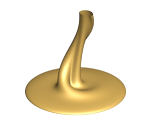
Figure 1. (a) Schematic of the computational domain with the temperature iso-surface ( $T=0.1$) of a thermal plume in its periodic state at
  $Ra=1.5\times 10^6$, in which the centre of the coordinate system aligns with the centre of the heated surface. The dashed lines denote open boundaries adopted in numerical simulations. (b) The probing points
  $P_1=(0, 0, 0.01)$ and
  $P_2=(0, 0, 0.2)$ and lines are used in the following figures. The region highlighted in red denotes the heated surface; the grey part is the adiabatic wall. Line-v denotes a vertical line leaving the centre of the heated surface; line-r and line-c denote radial and circumferential lines, respectively.
According to (2.2)–(2.5), the non-dimensional governing equations are dominated by two controlling parameters, the Rayleigh number ( $Ra$) and the Prandtl number (
 $Pr$), defined as
 \begin{equation} Ra=\frac{g\beta\,\Delta T\,D^3}{\nu\kappa},\quad Pr=\frac{\nu}{\kappa}, \end{equation}
where  $g$ is gravitational acceleration,
  $\beta$ is the coefficient of thermal expansion and
  $\nu$ is the kinematic viscosity.
2.2. Geometry, boundary conditions and grid
In this study, the working fluid is water ( $Pr=7$), which is treated as an incompressible Newtonian fluid. As shown in figure 1(a), the flow develops on a heated circular rigid surface of diameter of
  $D$ that is enclosed by a cylindrical open boundary with diameter of
  $2D$ and height of
  $D$.
$D$.
The following initial and boundary conditions are adopted to investigate the transition and instability of the thermal boundary layer and plume on an isothermally rigid horizontal surface. Here, the bottom boundary is modelled as a no-slip rigid wall with isothermal heating condition for the heated surface and adiabatic condition on the annular extension, which can be written as
 \begin{gather} \left.\begin{gathered} {u}(x, y, 0, t) = {v}(x, y, 0, t)={w}(x, y, 0, t)=0,\\ T(x, y, 0, t)=1\quad \text{for}\ (x^2+y^2)^{{1}/{2}}\leq\tfrac{1}{2}, \end{gathered}\right\} \end{gather}
 \begin{gather} \left.\begin{gathered} {u}(x, y, 0, t) = {v}(x, y, 0, t)={w}(x, y, 0, t)=\frac{{\partial} T(x, y, 0, t)}{{\partial} z}=0\\ \text{for}\ \tfrac{1}{2}<(x^2+y^2)^{{1}/{2}}\leq1. \end{gathered}\right\} \end{gather}
The side and top boundaries of the computational domain are set as open boundaries using pressure outlet conditions, which can be given as
 $$\begin{gather} \frac{{\partial} {u}(x, y, z, t)}{{\partial} n}=\frac{{\partial} {v}(x, y, z, t)}{{\partial} n}= \frac{{\partial} {w}(x, y, z, t)}{{\partial} n} =0\quad \text{for}\ (x^2+y^2)^{{1}/{2}}=1, \end{gather}$$
 $$\begin{gather}\frac{{\partial} {u}(x, y, 1, t)}{{\partial} z}=\frac{{\partial} {v}(x, y, 1, t)}{{\partial} z}=\frac{{\partial} {w}(x, y, 1, t)}{{\partial} z} =0, \end{gather}$$
where  $n$ is the normal direction to the side boundary. The pressure outlet condition just determines the static pressure at the outlet boundaries and also allows the backflow to exist. All other flow quantities are extrapolated from the interior. Thus, the side and top boundaries can be seen as free flow conditions without sidewalls. Besides, the temperature of the inflow at open boundaries is set to the ambient temperature of
  $T=0$, while the temperature of the outflow at open boundaries can be solved. The initial condition of the flow may be motionless and isothermal (or may be the numerical results at different Rayleigh numbers), which gives
 \begin{equation} u(x, y, z, 0) = v(x, y, z, 0)=w(x, y, z, 0)=T(x, y, z, 0)=0. \end{equation}
2.3. Numerical simulation methods
The governing equations are solved using the finite volume method with the SIMPLE scheme. The advection term is discretized by the QUICK scheme, the diffusion term is discretized by a second-order central-difference scheme, and the transient term is discretized by a second-order backward implicit time-marching scheme. This numerical method is used successfully in other studies (Qiao et al. Reference Qiao, Tian, Nie and Xu2018; Jiang et al. Reference Jiang, Nie, Zhao, Carmeliet and Xu2021).
In order to make the grid lines ‘O’ shaped to reduce the skewness of block corners on continuous curves and also to eliminate the coordinate singularity in the centre of the domain, an O-type multi-grid system is established in Cartesian coordinates in which finer grids are applied in the region close to boundaries, and coarse grids in other regions, as shown in figure 2. Such a non-uniform grid system can be used to satisfactorily resolve the regions where larger velocity and temperature gradients are expected to occur.

Figure 2. (a) Top view of the O-grid system discretizing the computational domain, (b) zoomed-in top view of the O-grid system discretizing the computational domain of the red box in (a).
A series of tests are carried out to find the optimal time step, grid and domain size to ensure computing accuracy and the use of affordable computing resources. Four different grid systems with 0.5 million, 1 million, 2 million and 8 million cells, along with three non-dimensional time steps of 0.0005, 0.001 and 0.002 are tested in the case for  $Ra=6.0\times 10^7$. That is, since the critical Rayleigh number is approximately
  $Ra=5.02\times 10^7$ for which the flow becomes chaotic, the Rayleigh number of
  $Ra=6.0\times 10^7$ larger than and close to the critical value is selected to test the time step, grid and domain size to make sure that the numerical results satisfy the computing accuracy for the whole range of Rayleigh numbers. In
  $x$ and
  $y$ directions, the grid system is constructed with
  $\Delta x=\Delta y=0.007$ with an expansion factor of 1.04 (growth rate of the cell length from one cell to the next) from the centre to the boundary edge. In the
  $z$ direction, the grid is constructed with
  $\Delta z=0.007$ and an expansion factor of 1.06 from the bottom to the top boundary. The temperature and velocity in the cases with different grid systems and time steps are monitored at point
  $P_1=(0, 0, 0.01)$, as illustrated in figure 1(b). The average temperature and velocity as well as the relative variations with the reference solution of test 2 are listed in table 1. Based on the results in table 1, the velocity variation is 3.5 %, 0.7 % and 1.1 % between tests 1, 3 and 4 and test 2, respectively. Furthermore, the velocity variation between test 2 and tests 5 and 6 is small. Therefore, the case of test 2 with the grid system of 1 million cells and time step of 0.001 is adopted as the best option, given both computing accuracy and cost.
Table 1. Average  $z$-velocity and temperature at point
  $P_1=(0, 0, 0.01)$ for
  $Ra=6.0\times 10^7$, using different numbers of cells and time steps.

In order to make sure that the open boundaries do not influence the buoyant flows, tests of different sizes of the computational domain are conducted. That is, the size of the domain is diameter of  $2D$ and height of
  $D$ in test 2, diameter of
  $2D$ and height of
  $2D$ in test 7, and diameter of
  $4D$ and height of
  $2D$ in test 8. As shown in table 2, all variations of the temperature and velocity between reference test 2 and other tests are less than 1 %. Since the flow in the thermal boundary layer and the plume stem is near the surface centre, the domain of
  $2D\times D$ is sufficiently large to capture the characteristics and structures of the transitional flows and is adopted in this study under consideration of accuracy and cost.
Table 2. Average  $z$-velocity and temperature at point
  $P_1=(0, 0, 0.01)$ for
  $Ra=6.0\times 10^7$, using different domain sizes.

For a further validation, figure 3 shows numerical results calculated using the present numerical simulation method and experimental data from Khrapunov, Potechin & Chumakov (Reference Khrapunov, Potechin and Chumakov2017). That is, the profile of the local Nusselt number ( $Nu_R=({R}/{(T_0-T_w)})({{\partial } T}/{{\partial } n})$, where
  $R$ is the radius of the disk) along the disk radius is calculated and presented at
  $Ra=3.78\times 10^6$ (or
  $Gr=5.40\times 10^6$). Clearly, the numerical results agree with experimental data from Khrapunov et al. (Reference Khrapunov, Potechin and Chumakov2017), suggesting that the present numerical method is guaranteed to describe the buoyant flows on the surface.

Figure 3. Validation of the local Nusselt number from the present numerical method with experimental results from Khrapunov et al. (Reference Khrapunov, Potechin and Chumakov2017) at  $Ra=3.78\times 10^6$, where
  $R$ is the radius of the disk.
3. Results and discussion
To unravel the transition route of the buoyant flows on the horizontal surface, hundreds of cases for  $Ra=10^1\hbox{--}6.0\times 10^7$ were calculated to distinguish various bifurcations, flow structures and corresponding critical values (critical Rayleigh numbers).
With increasing  $Ra$, the buoyant flows on the horizontal surface are observed to go through a series of bifurcations, starting with the conduction dominated flow, followed by a steady flow, a periodic flow with different states such as puffing, rotating and flapping, then a period-doubling flow and finally transition to chaos. Since a rotating state found in the transition route was rarely discussed in previous studies, we performed initial condition perturbation and direct stability analysis to further understand the rotating state. Random perturbations were imposed on the heated surface to understand the response of the buoyant flows in different transitional states.
3.1. The transition route to chaos
3.1.1. Basic flow
Starting off with  $Ra=10^1$, heat transfer is dominated by conduction from the heated surface to the fluids in a very weak flow. As shown in figure 4, there is no distinct thermal boundary layer or plume, but a steady axisymmetric dome structure. With increasing
  $Ra$ from
  $10^1$ to
  $10^3$, a noticeable convection starts to establish, which leads to the shrinking of the dome structure, where the high temperature region contracts and concentrates towards the centre of the dome.

Figure 4. The  $x$–
$x$– $z$ plane temperature contour plot of conduction-dominated flow at
  $t=50$ for (a)
  $Ra=10^1$, (b)
  $Ra=10^2$, (c)
  $Ra=10^3$; and temperature iso-surface at
  $T=0.1$,
  $t=50$ for (d)
  $Ra=10^1$, (e)
  $Ra=10^2$, (f)
  $Ra=10^3$.
For relatively larger  $Ra$, the convection effect becomes much more pronounced, which takes place over the dominance of the conduction effect. The thermal boundary layer and plume can be readily distinguished in figure 5. The radial temperature gradient and baroclinic effect drive the fluid radially inward and rise upward due to the buoyancy effect, finally forming a distinct plume. The temperature of the plume decreases with increasing height because of the dissipation of heat from the plume to the ambient fluid in the process of plume rising. With increasing
  $Ra$, the thicknesses of the thermal boundary layer and plume reduce, respectively. This is because the convection effect becomes stronger, leading to a larger temperature gradient. The heat transfer in this case is more intense, which is compatible with the scaling laws obtained for a heated horizontal surface model in Jiang, Nie & Xu (Reference Jiang, Nie and Xu2019b). As shown in figure 5, the flow is still steady and axisymmetric.

Figure 5. The  $x$–
$x$– $z$ plane temperature contour plot of convection-dominated flow at
  $t=50$ for (a)
  $Ra=10^4$, (b)
  $Ra=10^5$, (c)
  $Ra=10^6$; and temperature iso-surface at
  $T=0.1$,
  $t=50$ for (d)
  $Ra=10^4$, (e)
  $Ra=10^5$, (f)
  $Ra=10^6$.
For the purpose of illustrating the three-dimensional flow explicitly, time series of temperature profile are presented in vertical axial, radial and circumferential directions, as shown in figure 6. As illustrated in figure 1(b), the vertical line-v originates from the original point and ends at the centre of the top boundary. The radial line-r goes across the centreline and its length is  $4D/5$. The circumferential line-c diameter is also
  $4D/5$. Line-r and line-c are both
  $D/30$ height away from the bottom boundary. Note that at this height, the temperature profiles can describe the structures of both thermal boundary layer and thermal plume more completely. Especially, in the circumferential direction,
  $\theta$ refers to the non-dimensional angle of the circle from 0 to 360
 $^\circ$. For better understanding, we trim and stretch the circle into a straight line and depict the temperature profiles along it. In different directions, the variation of complex flow structures with increasing Rayleigh number can be distinguished clearly.

Figure 6. Temperature time series in (a) vertical, (b) radial and (c) circumferential directions, as illustrated in figure 1(b) for  $Ra=1.0\times 10^6$.
When  $Ra=1.0\times 10^6$, the flow is in a steady state. In the vertical direction in figure 6(a), the temperature declines with increasing height. The heat is transferred from the heated surface into the surrounding fluid by convection and conduction. In figure 6(b), the temperature decreases from the centre to the edge of the surface in the radial direction because the horizontal flow in the thermal boundary layer is heated continuously by the surface. However, the temperature is uniform in the circumferential direction in figure 6(c), because the flow is axisymmetric. Additionally, the temperatures remain constant with time as the flow is in the steady state.
3.1.2. Hopf bifurcation: periodic puffing flow
With further increasing  $Ra$, a Hopf bifurcation occurs, triggering the buoyant flows to transit from steady to periodic state. The flow structures characterized by temperature contours of a complete cycle in
  $x$–
$x$– $y$ and
  $x$–
$x$– $z$ planes at different times are shown in figure 7, from which the evolution of the thermal boundary layer and plume can be readily observed. As
  $Ra$ increases, the radial flow in the thermal boundary layer driven by the baroclinic effect speeds up and the fluid carried away by the rising plume is less than the fluid accumulated due to the radial flow, which leads to the formation of a convective roll. The convective roll sheds from the thermal boundary layer, and it is entrained by the rising plume. After the departure of the convective roll, the flow from the edge of the plate fills in so that the process repeats over time, resulting in a periodic flow that is called the ‘puffing’ state, as illustrated in List (Reference List1982).

Figure 7. The  $x$–
$x$– $z$ plane temperature contour plot for
  $Ra=1.1\times 10^6$ at equilibrium state for one period at (a)
  $t+5.3$, (b)
  $t+5.7$, (c)
  $t+6.4$, (d)
  $t+7.3$. The
  $x$–
$x$– $y$ plane temperature contour plot at height
  $0.01D$ for
  $Ra=1.1\times 10^6$ at equilibrium state for one period at (e)
  $t+5.3$, (f)
  $t+5.7$, (g)
  $t+6.4$, (h)
  $t+7.3$.
As shown in figure 7(a), the flow structure in the puffing state is an axisymmetric plume. A puffing forms in the thermal boundary layer on the outer side of the thermal plume in the  $x$–
$x$– $z$ plane, which is produced by the strong buoyant flows from the edge of the heated circular surface in figure 7(b). The puffing is finally convected to the rising plume, as shown in figure 7(c). In fact, the puffing evolves into a convective roll in the thermal boundary layer around the thermal plume, as shown in figure 7(e). As the puffing moves towards the thermal plume, the convective roll also shrinks in the
  $x$–
$x$– $y$ plane, as depicted in figures 7(e,f). According to the temperature contour plot in the
  $x$–
$x$– $z$ plane, the puffing forms periodically on the edge of the thermal boundary layer, which can be illustrated from the multiple convective rolls in the
  $x$–
$x$– $y$ plane. The temperature contour and iso-surface can be seen in supplementary movies 1 and 2, available at https://doi.org/10.1017/jfm.2024.453.
As shown in figure 8(a), the time series of temperature profile becomes periodic for  $Ra=1.1\times 10^6$ in the vertical direction. The magnitude of the temperature fluctuates and peaks when the puffings merge into the plume and drops when the plume rises up. Periodic stripes appear with time in figure 8(b), implying that the flow is in a periodic state. According to the radial temperature profile, the stripes (puffings) appear simultaneously on both sides of the radial line. In the circumferential direction, the temperature is constant on the circle in the same time, proving that it is also a symmetric state.

Figure 8. Temperature time series in (a) vertical, (b) radial and (c) circumferential directions, as illustrated in figure 1(b) for  $Ra=1.1\times 10^6$. (d) Two-dimensional Fourier transform of the radial temperature in (b) for
  $Ra=1.1\times 10^6$ with the peak
  $(f,k,P)=(0.415,800.781,0.118)$, where
  $f$ and
  $k$ are frequency and wavenumber respectively, and
  $P$ is the power spectral density.
Additionally, the two-dimensional Fourier transform (2-DFT) is used to study both temporal and spatial development of the flows. While the temperature profiles in the radial direction can generally describe the buoyant flows, the 2-DFT is applied on the temperature profiles in the radial direction to obtain both frequency and wavenumber at different Rayleigh numbers. The 2-DFT is performed on a long time period to ensure the accuracy of the results.
Figure 8(d) plots the 2-DFT results for  $Ra=1.1\times 10^6$. The power spectral density is defined as
 \begin{equation} P=\lvert\, fft(w)\rvert^2/(N\cdot\,f_s), \end{equation}
where  $fft(w)$ is to perform Fourier transform to vertical velocity,
  $N$ is the length of data and
  $f_s$ is the sampling frequency. It is clear that one distinct peak appears, indicating its fundamental frequency (non-dimensionalized by
  $(\kappa \,Ra^{1/2})/D^2$)
  $f_f=0.415$, and wavenumber
  $k=800.781$. It is clear that the solution loses its stability and bifurcates into a periodic solution by means of Hopf bifurcation.
3.1.3. Symmetry-breaking bifurcation: periodic rotating flow
In this study, when  $Ra$ increases to
  $1.9\times 10^6$, the periodic puffing state becomes unstable and a different periodic solution presented as a rotating state is observed. As shown in figure 9, the plume begins to rotate in anticlockwise order, as a consequence of which the flow becomes asymmetric. In this rotating state, the puffings do not appear simultaneously in the thermal boundary layer as they do in the puffing state. Instead, they appear on one side and rotate around the
  $z$-axis. The plume in the centre has quite a large heat flux going upwards at this
  $Ra$, which entrains the puffings around it. That is, the asymmetry of the puffings leads to this type of the rotating plume. The temperature contour and isosurface can be seen in supplementary movies 3 and 4.

Figure 9. The  $x$–
$x$– $y$ plane temperature contour plot at height
  $0.01D$ for
  $Ra=2.0\times 10^6$ at equilibrium state for one period at (a)
  $t+4.6$, (b)
  $t+5.2$, (c)
  $t+5.8$, (d)
  $t+6.4$. The temperature iso-surface for
  $T=0.1$ and
  $Ra=2.0\times 10^6$ at equilibrium state for one period at (e)
  $t+4.6$, (f)
  $t+5.2$, (g)
  $t+5.8$, (h)
  $t+6.4$. The arrow denotes that the flow rotates in anti-clockwise direction.
Clearly, when an equilibrium state undergoes a symmetry-breaking bifurcation, new fluid flow states appear with less symmetry and more sophisticated dynamics. According to the study of Crawford & Knobloch (Reference Crawford and Knobloch1991), if a system remains unchanged under arbitrary rotation around the central axis and with reflections over any vertical plane through the central axis, the symmetry group of solutions to the governing equations under such boundary conditions is termed the group  $O(2)$. Breaking
  $O(2)$ symmetry can lead to either standing or rotating waves when the bifurcating eigenvalue is complex. Furthermore, because of the reflection symmetry, the rotating state can be in the clockwise or anticlockwise direction; both solutions bifurcate simultaneously, one of which can be observed, dependent on initial conditions. Most rotating flows are generated through symmetry breaking, as also observed in the stratified fluid in a closed cavity (Murphy & Lopez Reference Murphy and Lopez1984; Navarro & Herrero Reference Navarro and Herrero2011).
The circumferential velocity can be used to distinguish the rotating flows. When the circumferential velocity at one point inside the plume but away from the vertical axis is zero, the flow has no velocity in circumferential direction and thus moves directly upwards without rotation. When the plume begins to rotate in a specific direction, the circumferential velocity will be non-zero. In figure 10, the circumferential velocity is near zero when  $Ra$ is smaller than
  $1.7\times 10^6$, but increases slightly at
  $Ra=1.8\times 10^6$, suggesting that the solution tends to become unstable and potentially approaches the critical value. After the circumferential velocity suddenly rises to 0.018 at
  $Ra=1.9\times 10^6$, the flow becomes asymmetric and this symmetry-breaking process is responsible for the propagation of rotation. It is worth noting that there is a large variance of the circumferential velocity between
  $Ra=1.8\times 10^6$ and
  $1.9\times 10^6$. Accordingly, it may be expected that the bifurcation to the rotating state occurs at
  $Ra=1.9\times 10^6$. It is clear that the circumferential velocity decreases again but will not be zero, as shown in figure 10, because the flapping flows in § 3.1.4 still have circumferential velocity, which is not as strong as that of the rotating flows.

Figure 10. Velocity in the circumferential direction for different Rayleigh numbers.
As shown in figure 11(a), the temperature decreases sharply in the vertical axial direction and the puffing stripes can be hardly distinguished. That is mainly because in the rotating state, the plume rotates around the centre, rather than stationarily appearing at the centre location. As a result, the temperature gradient is quite large in the centre. Given the temperature profile in the other two directions, the puffings appear alternately on different sides of the radial line, which means that the flow is no longer symmetric, as shown in figure 11(b). Further, as depicted in figure 11(c), the temperature at the end of this period is the same as that at the beginning of the next period, which suggests that the plume rotates around the circle. Figure 11(d) shows the 2-DFT results for  $Ra=2.0\times 10^6$. Clearly, the flow in the rotating state is still periodic with discernable harmonic modes. The fundamental frequency of the rotating state (
 $\,f_f=0.452$) is slightly larger than that of the puffing state (
 $\,f_f=0.415$), indicating that the fundamental frequency and wavenumber increase with the Rayleigh number.

Figure 11. Temperature time series in (a) vertical, (b) radial and (c) circumferential directions, as illustrated in figure 1(b) for  $Ra=2.0\times 10^6$. (d) The 2-DFT of the radial temperature in (b) for
  $Ra=2.0\times 10^6$ with the peak
  $(f,k,P)=(0.452,1113.28,0.375)$, where
  $f$ and
  $k$ are frequency and wavenumber, respectively, and
  $P$ is the power spectral density.
3.1.4. Reflection-symmetric state: periodic flapping flow
With increasing  $Ra$, the periodic rotating state breaks but a periodic flapping state with reflection symmetry occurs between
  $Ra=2.1\times 10^6$ and
  $Ra=2.2\times 10^6$. The flow structure is also different from the structures presented in figure 7. Figures 12(a–h) show that the puffings form alternately at the ‘two sides’ (outer region) of the plume in the thermal boundary layer; that is, the convective roll is not symmetric, different from those in the periodic puffing state in figure 7. The tilted puffings make the plume far away from the
  $z$-axis at the centre, leading to a ‘flapping’ plume.

Figure 12. The  $x$–
$x$– $z$ plane temperature contour plot for
  $Ra=2.5\times 10^6$ at equilibrium state for one period at (a)
  $t+3.8$, (b)
  $t+4.4$, (c)
  $t+5.0$, (d)
  $t+5.6$. The
  $x$–
$x$– $y$ plane temperature contour plot at height
  $0.01D$ for
  $Ra=2.5\times 10^6$ at equilibrium state for one period at (e)
  $t+3.8$, (f)
  $t+4.4$, (g)
  $t+5.0$, (h)
  $t+5.6$. The arrow denotes that the flow flaps in this direction.
It is worth noting that in the flapping state, the reflection symmetry is still preserved, while the rotational symmetry has been broken. The buoyant flows are symmetrical with the vertical plane through the central axis, as illustrated by the dashed lines in figures 12(e–h). That is, this kind of asymmetrical convective roll makes the plume flap in a certain direction, as shown in the top view of the temperature contours in the  $x$–
$x$– $y$ plane. The temperature contour and iso-surface can be seen in supplementary movies 5 and 6.
Figure 13 plots temperature time series in vertical, radial and circumferential directions for  $Ra=2.5\times 10^6$. The stripes can be distinguished clearly in the vertical direction, as shown in figure 13(a). The temperature difference between different stripes is also larger than that in the puffing state due to the flapping of the plume. When the plume sways to the edge of the heated surface, the temperature at the centreline decreases significantly. In the radial direction, the puffings appear alternately on different sides of the radial line, and the plume in the centre sways to the left and right to interact and merge with the puffings on different sides, which is referred to as a flapping state. In figure 13(c), the temperature in the circumferential direction is not spatially homogeneous at the same time. The stripes turn into a ‘wave’ shape, and the wave evolves with the change of time, suggesting that the flow is periodic but asymmetric. Figure 13(d) shows that the fundamental frequency of the flapping state is 0.464, which proves that the flapping flow is still under a periodic state. The wavenumber of the flapping state is the same as that of the rotating state.

Figure 13. Temperature time series in (a) vertical, (b) radial and (c) circumferential directions, as illustrated in figure 1(b) for  $Ra=2.5\times 10^6$. (d) The 2-DFT of the radial temperature in (b) for
  $Ra=2.5\times 10^6$ with the peak
  $(f,k,P)=(0.464,1113.28,0.889)$, where
  $f$ and
  $k$ are frequency and wavenumber, respectively, and
  $P$ is the power spectral density.
The fundamental frequency varies under different flow states, as shown in figure 14. The fundamental frequency of the flapping state is similar to that of the rotating state but larger than that of puffing state. The similar fundamental frequency of the rotating and flapping states implies that the flapping and rotating flows have similar time-dependent characteristics.

Figure 14. Fundamental frequency for different Rayleigh numbers.
3.1.5. Period-doubling bifurcation
Figure 15 shows the temperature contours at  $Ra=6.5\times 10^6$. Clearly, the second roll (CR2) interacts with the first roll (CR1) before the first one vanishes. That is, there are two small periods in one complete cycle, which is the period-doubling bifurcation. The flow remains a flapping state, but sways in a different direction compared to that in the periodic state in e.g. figure 12. Note that the difference between the two swaying directions is quite small and hard to distinguish in these figures. The swaying direction of the plume depends on the initial conditions. Additionally, the flapping plume does not sway on the whole heated plate as it does in the periodic flapping state, but sways in a small region, as shown in figures 15(a–d). That is mainly because with the Rayleigh number increasing, the characteristic length of the heated surface that we observed in the flow field also becomes bigger. According to the definition of
  $Ra$, the characteristic length will have growth factor of 1.38 with the increasing of
  $Ra$ from
  $2.5\times 10^6$ to
  $6.5\times 10^6$, which means that the flapping region will have reduction factor of 0.74. As a result, the flapping on the whole heated plate shrinks into a small region. Additionally, two puffings form successively and merge into one puffing near the centre, which is different from the periodic flapping state. According to the temperature contours in figures 15(e–h), two convective rolls (CR1 and CR2) exist simultaneously and are then entrained by the plume and flow upwards, which may explain why the period doubles in this state.

Figure 15. The  $x$–
$x$– $z$ plane temperature contour plot for
  $Ra=6.5\times 10^6$ at equilibrium state for one period at (a)
  $t+2.9$, (b)
  $t+5.2$, (c)
  $t+7.5$, (d)
  $t+9.8$. The
  $x$–
$x$– $y$ plane temperature contour plot at height of
  $0.01D$ for
  $Ra=2.5\times 10^6$ at equilibrium state for one period at (e)
  $t+2.9$, (f)
  $t+5.2$, (g)
  $t+7.5$, (h)
  $t+9.8$. The convective rolls are pointed out in the plot as CR1 and CR2.
Figure 16 shows temperature time series in vertical, radial and circumferential directions for  $Ra=6.5\times 10^6$. As shown in figure 16(a), the period is apparently longer than that of the periodic flow shown in figure 8(a). Two stripes appear in one period, which can be described as a period-doubling state. A different type of flow structure appears in the radial direction. First, a puffing appears at the edge of the heated surface and moves to the plume. Before it arrives at the centre, another puffing also appears and moves just like the previous one. Two puffings meet and merge into one puffing, moving towards the plume and finally being entrained by the plume. As shown in figure 16(b), two stripes meet in the process of flowing towards the centre, and become one stripe. The plume in the centre sways to its left and right, which makes this state an asymmetric flow. This special flow structure is the combination of the puffing and flapping states. In the circumferential direction, the temperature profile is more like an axisymmetric puffing state, as shown in figure 16(c). That is mainly because the circle chosen in the circumferential direction is close to the edge of the heated horizontal surface, where the flow structure captured on this circle is only the puffings flowing away from the centre. For the period-doubling flow in figure 16(d), another peak at a frequency of
  $f_f/2=0.2075$ can be found under a different wavenumber due to interaction between waves (also see figure 16 and Drazin (Reference Drazin2002) for the period-doubling bifurcation).

Figure 16. Temperature time series in (a) vertical, (b) radial and (c) circumferential directions, as illustrated in figure 1(b) for  $Ra=6.5\times 10^6$. The black circles in the inset show the meeting points of puffs. (d) The 2-DFT of the radial temperature in (b) for
  $Ra=6.5\times 10^6$ with the peak
  $(f,k,P)=(0.415,839.8,0.721)$, where
  $f$ and
  $k$ are frequency and wavenumber, respectively, and
  $P$ is the power spectral density.
Figure 17 shows the temperature contours at  $Ra=3.0\times 10^7$. The buoyant flows above the surface at
  $Ra=3.0\times 10^7$ become axisymmetric again; that is, the plume in the centre no longer sways. With further increasing Rayleigh number to
  $Ra=3.0\times 10^7$, the flow is still in a period-doubling state. However, the flow structure differs from that at
  $Ra=6.5\times 10^6$. The puffings form simultaneously on the outer sides and then merge, before they are convected upwards by the plume, as shown in figures 17(a–d). That is, the convective rolls form at the edge of the heated surface and move inwards to the centre axis, which remains symmetric, as shown in figures 17(e–h).

Figure 17. The  $x$–
$x$– $z$ plane temperature contour plot for
  $Ra=3.0\times 10^7$ at equilibrium state for one period at (a)
  $t+3.0$, (b)
  $t+5.4$, (c)
  $t+7.8$, (d)
  $t+10.2$. The
  $x$–
$x$– $y$ plane temperature contour plot at height
  $0.01D$ for
  $Ra=2.5\times 10^6$ at equilibrium state for one period at (e)
  $t+3.0$, (f)
  $t+5.4$, (g)
  $t+7.8$, (h)
  $t+10.2$.
As shown in figure 18(a), the two stripes in the vertical direction at  $Ra=3.0\times 10^7$ are clearer compared to those at
  $Ra=6.5\times 10^6$, which means that the plume does not sway away from the centre but always puffs in the centre. The two stripes are very similar in one period. In the radial direction, the puffings also move the same as before (at
  $Ra=6.5\times 10^6$), but the central plume does not sway and the flow thus becomes axisymmetric again. As shown in figures 16(b) and 18(b), the temperature profiles in the radial direction at
  $Ra=6.5\times 10^6$ and
  $Ra=3.0\times 10^7$ are zoomed in for a better comparison and to understand what causes the change. Although one might reckon that the meeting point of two puffs at
  $Ra=6.5\times 10^6$ is the same as that in figure 18(b), the difference can be observed clearly in the insets of figures 16(b) and 18(b). The meeting points on the two sides are not the same in one period. This asymmetry of puffs finally affects the plume and makes the plume sway in different directions. However, at
  $Ra=3.0\times 10^7$, the meeting points are the same on both sides, which means that there is no symmetry-breaking effect on the plume.

Figure 18. Temperature time series in (a) vertical, (b) radial and (c) circumferential directions, as illustrated in figure 1(b) for  $Ra=3.0\times 10^7$. The black circles in the inset show the meeting points of puffs.
3.1.6. Transition to chaos
The buoyant flows above the horizontal surface become more complex and finally evolve into a chaotic state. Figure 19 displays the temperature contours of the chaotic state at  $Ra=5.02\times 10^7$ in the
  $x$–
$x$– $z$ plane. The plume in the centre is quite chaotic and presents flow structures of various length scales. However, the puffings near the edge of the plate still remain approximately ordered to some extent. According to Hattori et al. (Reference Hattori, Norris, Kirkpatrick and Armfield2013b), instability of the plume stem could be caused by Kelvin–Helmholtz instability. The stability characteristics of the thermal boundary layer flow appear to be affected by oscillations in the stem by a feedback mechanism. That is, the flow in the plume stem becomes randomly oscillatory with feedback to the thermal boundary layer flow. As a result, the flow in the thermal boundary layer is also chaotic with some periodic characteristics at the critical value of the bifurcation to chaos.

Figure 19. The  $x$–
$x$– $z$ plane temperature contour plot for
  $Ra=5.02\times 10^7$ at equilibrium state for one period at (a)
  $t+2.0$, (b)
  $t+3.5$, (c)
  $t+5.0$, (d)
  $t+7.5$.
According to the temperature profiles in figure 20(a), there is no distinct period of the plume and the stripes become irregular. However, the puffings still appear regularly at the edge of the heated surface in figure 20(b), which indicates that the flow has not entered a fully developed chaotic state. It also indicates that chaotic bifurcations occur first in the centre plume part and then in the boundary layer at the outer regions. As shown in figure 20(c), the stripes appear as small waves in the circumferential direction, suggesting that the puffings at the edges still have small differences in the circumferential direction and thus are not in a symmetric state. Additionally, the 2-DFT results of the chaotic flow in figure 20(d) show that there is no distinct fundamental frequency with more flow structures of different wavelengths.

Figure 20. Temperature time series in (a) vertical, (b) radial and (c) circumferential directions as illustrated in figure 1(b) for  $Ra=5.02\times 10^7$. (d) The 2-DFT of the radial temperature in (b) for
  $Ra=5.02\times 10^7$, where
  $f$ and
  $k$ are frequency and wavenumber, respectively, and
  $P$ is power spectral density.
3.1.7. The whole route to chaos
For better understanding of the route to a chaotic state, the trajectories from  $t_f$ to
  $t_f+30$ with about 12 cycles in the
  $u\hbox{--}w\hbox{--}T$ space are plotted in figure 21 for the typical flow states at point
  $P_1$ on the circular surface. The trajectory finally approaches a fixed point at
  $Ra=1.0\times 10^6$ at the steady state in figure 21(a), and a limit cycle at
  $Ra=1.1\times 10^6$ at the periodic puffing state in figure 21(b). For periodic rotating and flapping states at
  $Ra=2.0\times 10^6$ and
  $Ra=2.5\times 10^6$, the trajectory is also a limit circle, but to some extent twisted compared with the puffing case (figures 21c,d). A
  $T^2$ torus appears at
  $Ra=3.0\times 10^7$ in which the flow is in the period-doubling state in figure 21(e). Finally, the trajectory becomes a complex attractor at
  $Ra=5.02\times 10^7$ in which the flow is chaotic, as shown in figure 21(f).

Figure 21. The attractors of  $x$-velocity
  $u$,
$u$,  $z$-velocity
  $w$ and temperature
  $T$ at
  $P_1$ at
  $t_f$ to
  $t_f+30$ for (a)
  $Ra=1.0\times 10^6$, (b)
  $Ra=1.1\times 10^6$, (c)
  $Ra=2.0\times 10^6$, (d)
  $Ra=2.5\times 10^6$, (e)
  $Ra=3.0\times 10^7$, (f)
  $Ra=5.02\times 10^7$.
To identify the chaotic state, the maximum Lyapunov exponent ( $\lambda _L$) of the attractors in figure 21 is calculated, defined as (Odavić, Mali & Tekić Reference Odavić, Mali and Tekić2015)
 \begin{equation} \lambda_L = \frac{1}{t_n-t_0}\sum_{i=1}^{n}\ln\frac{d(t_i)}{d(t_{i-1})}. \end{equation}
In this equation,  $d(t_0)$ is the initial distance of two points selected in the orbit of the attractors (also see figure 21). For the next time
  $t_1=t_0+\Delta t$ (e.g.
  $\Delta t=100$ time steps), the two points arrive at new positions, and the distance between two points becomes
  $d(t_1)$. Further, we can find new points with a distance
  $d(t_0)$, and then we may start the next calculation and iterate several times (
 $n>50$). As shown in figure 22,
  $\lambda _L$ becomes larger than zero for
  $Ra\geq 5.02\times 10^7$, beyond which the flow enters the chaotic state (also see Odavić et al. (Reference Odavić, Mali and Tekić2015), for chaos described by the maximum Lyapunov exponent).

Figure 22. The maximum Lyapunov exponent  $\lambda _L$ for different Rayleigh numbers.
For further understanding of the heat transfer of the transitional flow on the heated circular surface, the Nusselt number on the horizontal surface is also calculated. As shown in figure 23, the Nusselt number of unsteady flows calculated from the present numerical results is consistent with experimental results from Kitamura & Kimura (Reference Kitamura and Kimura2008). With  $Ra$ increasing,
  $Nu$ also increases with the scaling law of
  $Nu\sim Ra^{1/4}$, which means that the heat transfer is enhanced with the increasing of
  $Ra$.
$Ra$.

Figure 23. Nusselt number of unsteady flows from numerical results and experimental data from Kitamura & Kimura (Reference Kitamura and Kimura2008).
3.2. Various states subjected to perturbations
As we discussed above, the onset of the transition usually goes through a series of bifurcations. Adding perturbations is one way to control different flow states and also control chaos (Shinbrot et al. Reference Shinbrot, Grebogi, Yorke and Ott1993; Markman & Bar-Eli Reference Markman and Bar-Eli1994). To examine the stability of the flow near the critical values and especially the stability of different flow states, the effect of initial condition on the bifurcation of the transitional flow is tested. The dependence of initial condition is also termed ‘hysteresis’ in the previous studies by e.g. Ridouane & Campo (Reference Ridouane and Campo2006) and Ma, Sun & Yin (Reference Ma, Sun and Yin2006), in which different flow states and critical values were obtained by increasing or decreasing  $Gr$ or
  $Ra$.
$Ra$.
In this study, numerical tests about how initial condition affects the bifurcation are performed, in which the solutions at critical values are obtained by using the results for other Rayleigh numbers as initial condition. For example, the results at  $Ra=1.1\times 10^6$ (periodic puffing state) are used as initial condition for the simulation at
  $Ra=1.0\times 10^6$ (steady state). As shown in table 3, in most cases, the change of initial condition does not change the flow characteristics except for the rotating state. When the numerical results of a periodic flapping state at
  $Ra=2.5\times 10^6$ are used as initial condition for the simulation of the periodic rotating flow at
  $Ra=2.0\times 10^6$, the flow finally becomes flapping because of the effect of initial condition (hysteresis effect). Further, when the numerical results of a periodic rotating state at
  $Ra=2.0\times 10^6$ are adopted as initial condition for the simulation of the periodic puffing flow at
  $Ra=1.8\times 10^6$, the flow will also become rotating. It is clear that the rotating state is easily affected by initial condition; that is, the rotating flow near the critical value has a distinct hysteresis effect (see Ma et al. (Reference Ma, Sun and Yin2006) for hysteresis effect).
Table 3. Tests of flow states using different initial conditions.

When the initial condition perturbation is added to the system at the beginning, it is easy to be dissipated during the development of the transitional flows. To examine the stability of the flows near critical values with persistent perturbations, a direct stability analysis is performed. That is, random numerical perturbations in both time and space are superimposed onto the boundary condition of the heated horizontal surface. The amplitude of random perturbations is  $5\,\%$ of the difference between the temperatures of the surface and ambient fluid. Furthermore, the effect of the perturbation amplitude is tested to guarantee that the response in the thermal boundary layer is in the linear regime (also see Zhao, Lei & Patterson (Reference Zhao, Lei and Patterson2013), for details).
Numerical results show that when  $Ra=0.9\times 10^6$, the flow is steady both with and without random perturbations. Random perturbations do not grow but decay when they travel downstream.
As shown in figure 6, the flow is also steady for  $Ra=1.0\times 10^6$. Further, we introduce random perturbations into the flow at
  $Ra=1.0\times 10^6$. However, numerical results show that the flow transits into a periodic state in which the bifurcation occurs at this
  $Ra$. That is, the flow is steady without random perturbations but periodic with random perturbations for which the decay of the periodic characteristics is compensated through the persistent perturbations. This means that the flow is conditionally stable at
  $Ra=1.0\times 10^6$.
Further, the puffing state is also tested through introducing random perturbations; that is, the calculation similar to that for  $Ra=1.0\times 10^6$ is repeated for
  $Ra=1.5\times 10^6$. The numerical results demonstrate that the flow of the puffing state is stable.
Additionally, the flow of the rotating state at  $Ra=2.0\times 10^6$ is also examined. Figure 24 shows the numerical results with random perturbations. Clearly, after superimposing random perturbations onto the heating boundary, the flow bifurcates from the rotating state in figure 24(a) to the flapping state in figure 24(b). That is, introducing random perturbations may alter the stability of the rotating state, advancing it to other states. For the purpose of understanding the influence of the perturbation amplitude, a series of random numerical perturbation tests are performed, with
  $1\,\%$,
  $2\,\%$,
  $3\,\%$,
  $4\,\%$,
  $5\,\%$ and
  $10\,\%$ of temperature difference as the random perturbation amplitude. Numerical perturbation tests show that when the perturbation amplitude is sufficiently large (
 ${>}3\,\%$), the rotating state can be disturbed and it enters a flapping state in advance at the same
  $Ra$, implying that the rotating state is conditionally stable, which is also dependent on initial condition as described above.

Figure 24. The  $x$–
$x$– $y$ plane temperature contour plot at height of
  $0.01D$ for
  $Ra=2.0\times 10^6$ at equilibrium state for (a) isothermal heating and (b) isothermal heating with superimposed perturbations.
With further increasing  $Ra$ to
  $6.4\times 10^6$ near the critical value for the bifurcation from the periodic flapping state to the period-doubling flapping state, random perturbations are also introduced to the heating boundary in numerical simulation. Numerical results show that the perturbed flow remains periodic rather than entering the period-doubling state. This is probably because the break of symmetry occurs more easily in the spatial domain but not in the temporal domain (e.g. from periodic to period-doubling).
In summary, perturbations may influence the stability of the flow on a heated horizontal surface; that is, the flow could be conditionally stable with hysteresis effect near the critical values. In the case for small  $Ra$, the perturbations may increase the complexity of the flow and lead the flow to bifurcate in advance to the next transition state. For example, in the rotating state, the flow is conditionally stable. When random perturbations of large amplitude are introduced, the rotating state transits to the flapping state. The whole transition route of the flow on a heated horizontal surface with the increasing of
  $Ra$ with and without random perturbations is shown in figure 25. Without perturbations, the flow goes through a series of bifurcations and has different flow structures, from steady to periodic puffing, rotating, flapping, period-doubling and finally chaos. However, with random perturbations, the flow may be affected by random perturbations and bifurcate into the next transition state such as from steady to periodic puffing and from periodic puffing to flapping without rotating state. It is worth noting that only perturbation tests of typical states are performed because of computing time and cost.

Figure 25. The transition route of the buoyant flow on a heated horizontal surface with the increasing of  $Ra$, in which the dashed line means the extension of the axis.
4. Conclusions
The critical transition route of the buoyant flows on an isothermally heated horizontal circular surface is investigated in this study using three-dimensional numerical simulations. The range of  $Ra$ is covered from
  $10^1$ to
  $6.0\times 10^7$ for
  $Pr=7$ (water). Apart from the transition route, the stability of different states is studied using direct stability analysis, in which the influence of random perturbations on transition is examined using numerical perturbation tests.
In the transition route of the buoyant flows, when  $Ra$ is less than
  $10^3$, the flow is under conduction dominance without presenting a distinct thermal boundary layer or starting plume, exhibiting a heat dome structure. When
  $Ra$ is larger, for instance in the range for
  $10^3< Ra<10^6$, the convective effect becomes more distinct and gradually dominates the flow, which results in the distinct rising plume while the flow is still steady and axisymmetric.
A Hopf bifurcation occurs as  $Ra$ is in the range from
  $1.0\times 10^6$ to
  $1.1\times 10^6$, resulting in a periodic puffing flow with puffings forming in the thermal boundary layer. The puffings are then entrained by the plume and convected upwards eventually. As
  $Ra$ increases further, the flow enters a unique periodic rotating state, and the symmetry of the flow is lost between
  $Ra=1.8\times 10^6$ and
  $Ra=1.9\times 10^6$. Next, the flow enters a periodic flapping state, which is not axisymmetric but is symmetric about the vertical plane only for
  $Ra$ between
  $2.1\times 10^6$ and
  $2.2\times 10^6$. When
  $Ra$ increases to
  $6.5\times 10^6$, a period-doubling bifurcation occurs and the period of the flow becomes twice as large as the period of the preceding state. Finally, the flow evolves into the chaotic state when
  $Ra$ is in the vicinity of
  $5.02\times 10^7$. This study is based on an isothermal heated boundary condition. However, there are certainly a number of applications for which an isoflux heated plate is relevant. According to Jiang, Nie & Xu (Reference Jiang, Nie and Xu2019a) and Jiang et al. (Reference Jiang, Nie and Xu2019b), the dynamics and heat transfer of natural convection on isothermal and isoflux heated surfaces are quite different, which can also lead to the difference in the transition route to chaos. The difference between different boundary conditions can also be investigated in the future.
Direct stability analysis is also conducted to understand different states. Initial condition perturbations and random numerical perturbations are superimposed on the system. We find that for the regimes near critical values for  $Ra=1.0\times 10^6$ and
  $Ra=2.0\times 10^6$, the flow is conditionally stable and it bifurcates to the next state in advance due to the perturbations. The direct stability analysis is focused on the temporal variation of the transitional flows. However, the spatial development of the perturbations, i.e. from upstream to downstream in different states, may be different (convective instability). The spatial characteristics are also worth investigating in future work.
Supplementary movies
Supplementary movies are available at https://doi.org/10.1017/jfm.2024.453.
Funding
The authors would thank the National Natural Science Foundation of China for financial support (no. 11972072). The simulations were undertaken with the assistance of resources from Euler Cluster, which is supported by the Chair of Building Physics at ETH Zurich.
Declaration of interests
The authors report no conflict of interest.
Data availability statement
All data are involved in the paper.


