


Nomenclature
Nomenclature
-
 ${a_o}$
-
projectile acceleration relative to the ground, constant,
${\rm{m/}}{{\rm{s}}^2}$
-
$|{a_o}|$
-
projectile acceleration magnitude,
${\rm{m/}}{{\rm{s}}^2}$
-
${A_{ref}}$
-
cross-sectional base area,
${{\rm{m}}^2}$
-
${c_d}$
-
steady state drag coefficient
-
${c_d}(t)$
-
unsteady drag coefficient due to acceleration or deceleration
-
$D$
-
base diameter, constant, mm
-
$F$
-
steady state drag force, N
-
$F(t)$
-
unsteady drag force due to acceleration or deceleration, N
- g
-
acceleration due to gravity = 9.81
${\rm{m/}}{{\rm{s}}^2}$
-
${L_c}$
-
conical-nose length, mm
-
${L_n}$
-
cylinder length, mm
- min./max.
-
minimum or Maximum
-
${\rm{M}}$
-
steady flight Mach number relative to the ground
-
${{\rm{M}}_i}$
-
initial Mach number relative to the ground
-
${{\rm{M}}_f}$
-
final Mach number relative to the ground
-
${\rm{M}}(t)$
-
unsteady flight Mach number relative to the ground
-
${{\rm{P}}_t}$
-
ambient static pressure, Pa
-
${q_o}$
-
ambient dynamic pressure steady state, Pa, =
$0.5\rho {{\rm{v}}^2}$
-
${q_o}(t)$
-
ambient dynamic pressure during acceleration or deceleration, Pa, =
$0.5\rho {(v(t))^2}$
- R
-
molecular gas constant for dry air = 287 J/kg.K
-
${\rm{R}}{e_d}$
-
Reynolds number based on
$D$
, =
$\frac{{\rho vD}}{\mu }$
or =
$\frac{{\rho uD}}{\mu }$
- ST
-
source Term,
${{\rm{S}}_e}$
and
${{\rm{S}}_m}$
-
${{\rm{S}}_e}$
-
energy source term =
$\rho \textrm{u}\frac{{du}}{{dt}}$
,
${\rm{W/}}{{\rm{m}}^3}$
-
${{\rm{S}}_m}$
-
momentum source term =
$\rho \frac{{du}}{{dt}}$
,
${\rm{N/}}{{\rm{m}}^3}$
-
$t$
-
elapsed time during accelerated flight, s
-
${{\rm{T}}_t}$
-
ambient static temperature, Pa
-
$u$
-
steady free stream fluid velocity relative to the projectile, m/s
-
${u_i}$
-
initial free stream fluid velocity relative to the projectile, m/s
-
$u(t)$
-
unsteady free stream fluid velocity relative to the projectile, m/s
-
$v$
-
steady flight velocity relative to the ground, m/s
-
${v_i}$
-
initial flight velocity relative to the ground, m/s
-
$v(t)$
-
unsteady flight velocity relative to the ground, m/s


Greek symbol
Greek symbol
-
$\gamma $
-
ratio of specific heat, for air = 1.4
-
$\Delta t$
-
time-step, s
-
$\theta $
-
cone half-angle,
$^ \circ $
-
$\rho $
-
density, kg/m3
-
$\mu $
-
viscosity, Pa.s


1.0 Introduction
Transient fluid dynamic effects in the transonic regime generate unique fluid behaviour during rapid acceleration when compared to a steady analysis. There is a change in the pressure loading upon the aerodynamic body during rapid acceleration (or deceleration) where well-known steady prediction methods for aerodynamic coefficients may not be accurate. Knowledge of changes in aerodynamic loads is valuable in obtaining increased agility and manoeuverability, and acceleration magnitudes of 100g, where g is the acceleration due to gravity, are common in missile applications where two cases are now described. The HiBEX (High Booster Experiment) missile attained peak axial acceleration of 400g and lateral acceleration of 60g [Reference van Atta, Reed and Deitchman8]. The 5th generation Denel Dynamics A-darter produced thru,st and lateral acceleration magnitudes of 200 and 60g, respectively [Reference Gledhill, Roohani, Forsberg, Eliasson and Nordström10].
It has been established that novel flow structures occur during significant acceleration or deceleration of an aerodynamic object. While the range of “significant acceleration” is yet to be quantified, earlier research found acceleration effects on a NACA0012 aerofoil in the transonic regime were strongly present at 100g, a value now common in missile manoeuvre. Examples described below include the persistence of detached bow shocks ahead of projectiles decelerating under drag in ballistic ranges to projectile speeds well below the speed of sound [Reference Saito, Hatanaka, Yamashita, Ogawa, Obayashi and Takayama1, Reference Kikuchi, Takayama, Igra, Falcovitz and Ben-Dor2, Reference Roohani, Gledhill, Mahomed and Skews4]; wake and separation shocks which overtake decelerating projectiles, changing the pressure at the stagnation point [Reference Mahomed, Roohani, Gledhill and Skews5]; and shocks that appear critical at Mach numbers well above the steady state equivalents in accelerated flow. As missiles are designed for more agility, it becomes increasingly necessary to provide an overview of the flow physics involved in these cases.
This study contributes to building a systematic understanding of significant acceleration effects such as shock wave propagation and development. A simple aerodynamic shape such as a cone-cylinder and one-dimensional motion are useful to describe the fundamental flow physics during rapid acceleration before proceeding to complex geometry or arbitrary motion. This article describes the unsteady transonic flow field and shock wave motion for a cone-cylinder during constant acceleration and deceleration.
Computational Fluid Dynamics (CFD) models are essential tools because arbitrary acceleration can be modelled, and detailed flow features can be explored, provided that the models are well validated. Suitable validation cases in the range of 100g and at transonic speeds are not common for two reasons. The first is that acceleration of air over a model in a wind tunnel is not equivalent to acceleration of an object in still air, given the necessary pressure gradient required to drive acceleration in a wind tunnel. The second is that suitable transonic data sets are rare in the public domain.
In the present work the free-flight portion from a ballistic range experiment was used to validate numerical techniques that simulate one-dimensional acceleration of an aerodynamic object through undisturbed air. The ballistic range experiments provide insight into unsteady shock wave motion during deceleration with approximately straight and level flight. A few suitable cases are reported in the literature for the transonic and supersonic regime [Reference Saito, Hatanaka, Yamashita, Ogawa, Obayashi and Takayama1, Reference Kikuchi, Takayama, Igra, Falcovitz and Ben-Dor2, Reference Yamashita, Fujiwara, Suzuki, Iwakaka, Sasoh, Mahomed, Roohani, Gledhill and Skews3].
Saito et al. [Reference Saito, Hatanaka, Yamashita, Ogawa, Obayashi and Takayama1] studied transonic deceleration of spheres with experimental and numerical methods. They showed that the bow shock continued to propagate ahead of the sphere, when the sphere, initially at a supersonic Mach number, had decelerated to the subsonic regime due to drag. This finding was demonstrated in detail by Kikuchi et al. [Reference Kikuchi, Takayama, Igra, Falcovitz and Ben-Dor2] in similar experiments.
More recently, ballistic range experiments by Yamashita et al. [Reference Yamashita, Fujiwara, Suzuki, Iwakaka, Sasoh, Mahomed, Roohani, Gledhill and Skews3] investigated the separation shock angle with boundary layer interaction for a hemisphere-cylinder-flare-cylinder projectile with Mach numbers of approximately 2.0. They showed that the separation shock angle decreased with increasing deceleration magnitudes, in the range of 800 to 1 600g. This ballistic range experiment was used to validate the numerical acceleration model implemented for this article.
Acceleration of aerofoils into stationary or stagnant air was investigated by Roohani and Skews [Reference Roohani and Skews6]. They studied acceleration and deceleration for an RAE2822 aerofoil pitched at 2.79 incidence, with constant acceleration magnitudes of approximately 10 and 100g. Acceleration effects were dominant for the transonic regime caused by flow history and unsteady shock wave motion relative to the aerofoil. Kumaravel et al. [Reference Kumaravel, Jeyajothiraj and Rathakrishnan7] investigated transonic shock wave position on a NACA0012 aerofoil during acceleration and deceleration into stationary air. Two constant acceleration magnitudes were tested, there were 5 and 10g. These studies confirmed acceleration effects were present for aerofoils at acceleration magnitudes as low as 10g. [Reference Gledhill, Forsberg, Eliasson, Baloyi and Nordström9, Reference Forsberg, Gledhill, Eliasson and Nordström16] demonstrated approximately 20% drop in the wave drag peak on a flare configuration accelerated at 4 500
 ${\textrm{m/}}{{\textrm{s}}^2}$
through the transonic range, but did not provide flow field conditions.
${\textrm{m/}}{{\textrm{s}}^2}$
through the transonic range, but did not provide flow field conditions.
A slender body of revolution (cone-cylinder) was chosen to study the primary effects of constant acceleration and deceleration in the transonic regime. To provide an understanding of the acceleration-related phenomena without the additional complexity of asymmetric base flow, the angle-of-attack was chosen to be
 ${0^ \circ }$
and the flow field was assumed to be axisymmetric. These assumptions lay a foundation for further studies to address non-zero angles of attack and more complex configurations.
${0^ \circ }$
and the flow field was assumed to be axisymmetric. These assumptions lay a foundation for further studies to address non-zero angles of attack and more complex configurations.
The numerical methodology and validation are described in Section 2. Drag results are shown in Section 3. The delayed development of shock waves during acceleration is shown in Section 4, while in deceleration, shocks propagate forward, overtaking the projectile, and contributing to significant changes in drag as described in Section 5.
2.0 Numerical methodology
2.1 Case description
The numerical requirement was to simulate acceleration of a cone-cylinder at zero angle-of-attack into stagnant air and through the transonic regime. Constant acceleration was modelled; an acceleration magnitude of 100g was chosen as a value at which to observe the fundamental-transonic flow physics relevant to missiles.
The cone-cylinder was accelerated from an initially steady Mach number,
 ${M_i}$
to a final Mach number
${M_i}$
to a final Mach number
 ${M_f}$
at
${M_f}$
at
 $|{a_o}|$
= 100g. The simulation time was 0.2ms. The simulation cases are summarised in Table 1.
$|{a_o}|$
= 100g. The simulation time was 0.2ms. The simulation cases are summarised in Table 1.
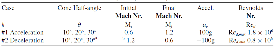
Cone-cylinder dimensions are diameter D = 50mm, and cylinder length
 ${L_c}$
= 250mm. Nose length
${L_c}$
= 250mm. Nose length
 ${L_n}$
varied with
${L_n}$
varied with
 $\theta $
and the slenderness ratio was (
$\theta $
and the slenderness ratio was (
 ${L_c}$
+
${L_c}$
+
 ${L_n}$
)/
${L_n}$
)/
 $(D)$
$(D)$
 $ \approx $
10. Ambient static pressure,
$ \approx $
10. Ambient static pressure,
 ${{\textrm{P}}_t}$
, and temperature,
${{\textrm{P}}_t}$
, and temperature,
 ${{\textrm{T}}_t}$
, were 101 325Pa and 300K, respectively.
${{\textrm{T}}_t}$
, were 101 325Pa and 300K, respectively.
2.2 Acceleration techniques
Simulation of an accelerating object can be carried out in an inertial reference frame (the frame of reference of an observer on the ground, for example), or in a non-inertial reference frame (the frame of reference attached to the accelerating object, for example). The Navier-Stokes equations hold in an inertial frame, but additional terms appear when they are transformed into a non-inertial frame [Reference Gledhill, Forsberg, Eliasson, Baloyi and Nordström9, Reference Combrinck and Dala14, Reference Musehane, Combrink and Dala17, Reference Forsberg18].
The ground distance covered during acceleration for Cases #1 and #2 in Table 1 at ambient conditions is approximately 60m for a which a grid or background corridor is required. Therefore, alternative numerical modeling methods were considered that does not require a background corridor.
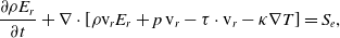
Table 1. Parameter description of the cone-cylinder simulation cases
 $^{\textrm{a}}$
Case #2, deceleration,
$^{\textrm{a}}$
Case #2, deceleration,
 $\theta { = 30^ \circ }$
was used for time-step convergence study.
$\theta { = 30^ \circ }$
was used for time-step convergence study.
 $^{\textrm{b}}$
Case #2, steady-state,
$^{\textrm{b}}$
Case #2, steady-state,
 ${{\textrm{M}}_i}$
= 1.2 was used for grid convergence study.
${{\textrm{M}}_i}$
= 1.2 was used for grid convergence study.
A description of the Navier-Stokes equations in both frames of reference is given in Appendix A constraint to rectilinear acceleration.
2.2.1 Moving reference frame acceleration technique
Consider a projectile whose fluid domain is a body-fixed grid accelerating relative to an inertial or absolute reference frame. Fluid velocities and accelerations for the body-fixed grid are expressed with respect to an absolute reference frame [15] and in absence of a background corridor. This is the basis for the Moving Reference Frame (MRF) acceleration technique where the Navier-Stokes, constitutive and turbulence equations are solved in the absolute reference frame.
The body-fixed grid is a non-inertial reference frame; Gledhill et al. [Reference Gledhill, Forsberg, Eliasson, Baloyi and Nordström9] provided a theoretical description of the general transform of the Navier-Stokes equations between the inertial (absolute) and non-inertial reference frames.
The instantaneous flight velocity,
 $v(t)$
is defined with respect to an absolute frame for the body-fixed grid and given as
$v(t)$
is defined with respect to an absolute frame for the body-fixed grid and given as
 $v(t) = {v_i} + {a_0}t$
, where
$v(t) = {v_i} + {a_0}t$
, where
 ${v_i}$
is the initial, flight velocity,
${v_i}$
is the initial, flight velocity,
 $t$
is the elapsed time from the start of accelerated flight, and
$t$
is the elapsed time from the start of accelerated flight, and
 ${a_0}$
is the projectile acceleration for constant, one-dimensional motion. The far-field boundary conditions are constant and
${a_0}$
is the projectile acceleration for constant, one-dimensional motion. The far-field boundary conditions are constant and
 $v(t)$
is specified for each body-fixed grid node. The unsteady flight Mach number is defined as M
$v(t)$
is specified for each body-fixed grid node. The unsteady flight Mach number is defined as M
 $(t) = {\textrm{v}}(t)/\sqrt {\gamma R{P_t}} $
.
$(t) = {\textrm{v}}(t)/\sqrt {\gamma R{P_t}} $
.
Since results displayed in the relative frame are more familiar to CFD users, results from the MRF acceleration technique are reported in the non-inertial, relative reference frame to maintain flow-field familiarity.
2.2.2 Source term acceleration technique
Consider a projectile whose fluid domain is a body-fixed grid. Projectile motion is described by the unsteady velocity function
 $u(t)$
, and modelled by holding the projectile stationary and the air accelerated relative to the projectile. The air is accelerated simultaneously for each grid cell and by the pressure-far-field boundary of the fluid domain, since no pressure gradient must exist across the fluid domain to generate acceleration of the air [Reference Roohani and Skews6]. This acceleration technique solves the Navier-Stokes, constitutive and turbulence equations in the relative, non-inertial reference frame by introducing appropriate source terms.
$u(t)$
, and modelled by holding the projectile stationary and the air accelerated relative to the projectile. The air is accelerated simultaneously for each grid cell and by the pressure-far-field boundary of the fluid domain, since no pressure gradient must exist across the fluid domain to generate acceleration of the air [Reference Roohani and Skews6]. This acceleration technique solves the Navier-Stokes, constitutive and turbulence equations in the relative, non-inertial reference frame by introducing appropriate source terms.
Energy (
 $\textrm{S}_{e} = \rho u\frac{{du}}{{dt}}$
in
$\textrm{S}_{e} = \rho u\frac{{du}}{{dt}}$
in
 ${\textrm{W/}}{{\textrm{m}}^3}$
) and Momentum (
${\textrm{W/}}{{\textrm{m}}^3}$
) and Momentum (
 ${{\textrm{S}}_m} = \rho \frac{{du}}{{dt}}$
in
${{\textrm{S}}_m} = \rho \frac{{du}}{{dt}}$
in
 ${\textrm{N/}}{{\textrm{m}}^3}$
) source terms are specified for constant, one-dimensional acceleration[19, 6, 9, 14]. The two source terms are added to the energy and momentum Navier-Stokes equations respectively through a User Defined Function feature in the solver. Source terms are applied to accelerate the air within each grid cell and a separate velocity function
${\textrm{N/}}{{\textrm{m}}^3}$
) source terms are specified for constant, one-dimensional acceleration[19, 6, 9, 14]. The two source terms are added to the energy and momentum Navier-Stokes equations respectively through a User Defined Function feature in the solver. Source terms are applied to accelerate the air within each grid cell and a separate velocity function
 $u(t) = - ({u_i} + {a_0}t)$
describes the acceleration of the air at the far-field boundary. The initial, free stream fluid velocity relative to the projectile is
$u(t) = - ({u_i} + {a_0}t)$
describes the acceleration of the air at the far-field boundary. The initial, free stream fluid velocity relative to the projectile is
 ${u_i}$
,
${u_i}$
,
 $t$
is the elapsed time from the start of accelerated flow and
$t$
is the elapsed time from the start of accelerated flow and
 ${a_0}$
now represents the fluid acceleration for constant, one-dimensional flight. Also,
${a_0}$
now represents the fluid acceleration for constant, one-dimensional flight. Also,
 $\frac{{du}}{{dt}}$
=
$\frac{{du}}{{dt}}$
=
 $ - {a_0}$
for definition of
$ - {a_0}$
for definition of
 ${{\textrm{S}}_e}$
and
${{\textrm{S}}_e}$
and
 ${{\textrm{S}}_m}$
.
${{\textrm{S}}_m}$
.
The flow physics for an object accelerating in free flight is equivalent to that for the same object kept stationary with every element of air accelerated over the object [Reference Roohani and Skews6]. Results from the Source Term (ST) acceleration technique are reported in the non-inertial, relative reference frame familiar from constant velocity simulations.
2.3 Solver description
ANSYS Fluent V.19.0 finite volume, compressible flow solver was chosen for implementation since it offered the solver, turbulence, transonic validation and user interfaces required for the acceleration, deceleration and steady models.
The solver configuration was implicit, density based and second-order accurate, with Roe-Flux Difference Splitting scheme for spatial discretisation and dual-time stepping for the unsteady formulation. The MRF one-dimensional acceleration model was used as described in subsection 2.2.
The minimum flight Reynolds number was
 ${\textrm{R}}{e_d}$
= 0.8
${\textrm{R}}{e_d}$
= 0.8
 $ \times $
10
$ \times $
10
 $^6$
based on
$^6$
based on
 ${{\textrm{M}}_i}$
and a maximum at 1.8
${{\textrm{M}}_i}$
and a maximum at 1.8
 $ \times $
10
$ \times $
10
 $^6$
based on
$^6$
based on
 ${{\textrm{M}}_f}$
. The
${{\textrm{M}}_f}$
. The
 ${\textrm{R}}{e_d}$
range was appropriate for the application of Menter’s SST (Shear Stress Transport) k-
${\textrm{R}}{e_d}$
range was appropriate for the application of Menter’s SST (Shear Stress Transport) k-
 $\omega $
turbulence model. This turbulence model was selected after testing of shock-induced boundary-layer separation occurring at Mach numbers near 0.90.
$\omega $
turbulence model. This turbulence model was selected after testing of shock-induced boundary-layer separation occurring at Mach numbers near 0.90.
Extensions from this investigation found that if
 ${\textrm{R}}{e_d}$
was approximately 500 000 or less, a transitional turbulence model was better suited for correct capture of the flow physics instead of a fully turbulent, Reynolds Averaged Navier-Stokes turbulence model under the same conditions.
${\textrm{R}}{e_d}$
was approximately 500 000 or less, a transitional turbulence model was better suited for correct capture of the flow physics instead of a fully turbulent, Reynolds Averaged Navier-Stokes turbulence model under the same conditions.
Grid adaption was applied every time-step to resolve shock waves and high gradient flow features. The adaption variables were static pressure, temperature, density and relative Mach number. Convergence studies to further confirm turbulence model, grid and time-step selection are discussed in the sub-sections to follow.
2.4 Grid detail
Figure 2 illustrates typical axisymmetric grids generated for the grid-convergence study. Pressure-far-field was applied to the domain boundary exterior, and the cone-cylinder surface was specified as a rigid wall. The domain limits were approximately 20 body-lengths in the length-wise and radial directions, measured about the cone-cylinder’s rotation axis.
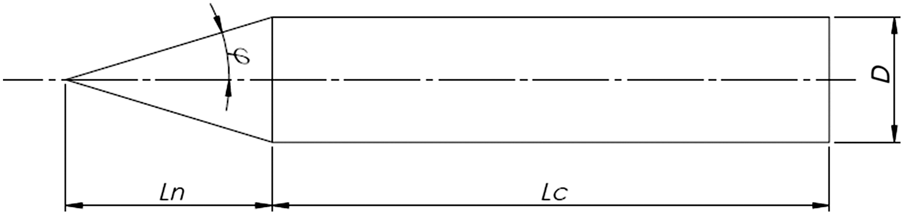
Figure 1. Cone-cylinder sketch with geometry definition. Dashed line indicates symmetry axis.
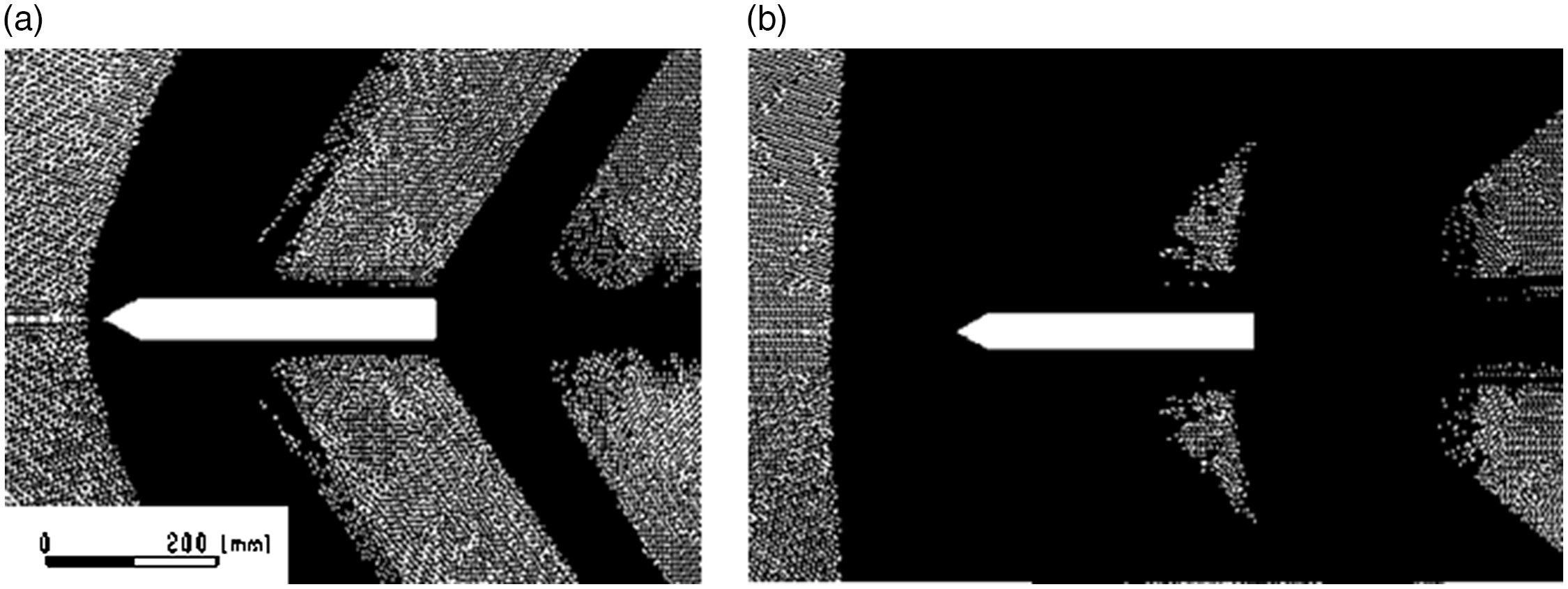
Figure 2. (a) Grid detail illustrated for steady state at M
 $ \approx $
1.2, and (b) instantaneous deceleration 100g at
$ \approx $
1.2, and (b) instantaneous deceleration 100g at
 ${\textrm{M}}(t) \approx $
0.9. Shaded regions indicate high grid density.
${\textrm{M}}(t) \approx $
0.9. Shaded regions indicate high grid density.
The axisymmetric grid consisted of unstructured tetrahedral elements and approximately 30 prism layers for the boundary layer. The first cell of the unadapted grid was located 1.8
 $ \times $
10
$ \times $
10
 $^{ - 4}$
mm from the wall boundary. The global mesh growth rate was 1.2, with a maximum cell skewness of 0.5. The
$^{ - 4}$
mm from the wall boundary. The global mesh growth rate was 1.2, with a maximum cell skewness of 0.5. The
 ${{\textrm{y}}^ + } \le 1$
condition for Menter’s SST k-
${{\textrm{y}}^ + } \le 1$
condition for Menter’s SST k-
 $\omega $
turbulence model was achieved for the entire wall boundary and for the Mach number range shown in Table 1.
$\omega $
turbulence model was achieved for the entire wall boundary and for the Mach number range shown in Table 1.
Approximately 1.5
 $ \times $
10
$ \times $
10
 $^6$
cells were typically used for the steady state solution (adapted), which increased to approximately 8
$^6$
cells were typically used for the steady state solution (adapted), which increased to approximately 8
 $ \times $
10
$ \times $
10
 $^6$
from transient grid adaption applied per time-step during deceleration.
$^6$
from transient grid adaption applied per time-step during deceleration.
2.5 Validation and convergence
Steady and unsteady solver validation was performed using a combination of numerical and experimental methods. Steady validation is discussed first, which compares steady simulation results to a wind tunnel experiment. This is followed by an unsteady validation, which compares unsteady MRF simulation with an alternative numerical technique and a unsteady free-flight portion from a ballistic range experiment. Transient convergence is demonstrated.
2.5.1 Steady
Steady state validation was demonstrated by numerically repeating a transonic wind tunnel experiment by Ramaswamy and Rajendra [Reference Ramaswamy and Rajendra11] with Menter’s k-
 $\omega $
SST turbulence model.
$\omega $
SST turbulence model.
This experiment investigated transonic flow past a blunt cone-cylinder at Mach 0.84 and
 ${\textrm{R}}{e_d}$
= 1.91
${\textrm{R}}{e_d}$
= 1.91
 $ \times $
10
$ \times $
10
 $^6$
, with boundary conditions
$^6$
, with boundary conditions
 ${{\textrm{P}}_t}$
= 172 369Pa and
${{\textrm{P}}_t}$
= 172 369Pa and
 ${{\textrm{T}}_t}$
= 300K. The numerical pressure profile measured in an axial direction was in good agreement with the experimental surface pressure measurement. This comparison of surface pressure is shown in Fig. 3. This result validated the solver’s steady state configuration, established suitability of the grid adaption parameter’s and confirmed the selected turbulence model was acceptable to resolve the dominant flow physics.
${{\textrm{T}}_t}$
= 300K. The numerical pressure profile measured in an axial direction was in good agreement with the experimental surface pressure measurement. This comparison of surface pressure is shown in Fig. 3. This result validated the solver’s steady state configuration, established suitability of the grid adaption parameter’s and confirmed the selected turbulence model was acceptable to resolve the dominant flow physics.
Figure 3. Steady state validation: wind tunnel surface pressure measured along the axial direction [Reference Ramaswamy and Rajendra11] compared with numerical results for Spalart-Allmaras and Menter’s k-
 $\omega $
SST turbulence models.
$\omega $
SST turbulence models.
Steady state simulations were performed for selected Mach numbers between
 ${{\textrm{M}}_i}$
and
${{\textrm{M}}_i}$
and
 ${{\textrm{M}}_f}$
from Table 1. These results resolved the salient flow features for a cone-cylinder in a transonic free-stream compared to experimental wind-tunnel data [Reference Solomon12, Reference Ericsson and Tucker13] for similar cone-cylinder geometries.
${{\textrm{M}}_f}$
from Table 1. These results resolved the salient flow features for a cone-cylinder in a transonic free-stream compared to experimental wind-tunnel data [Reference Solomon12, Reference Ericsson and Tucker13] for similar cone-cylinder geometries.
2.5.2 Unsteady
The MRF acceleration technique was validated using numerical and experimental methods. The numerical method is discussed first, followed by the experimental method.
The free-flight ballistic range experiment by Saito et al. [Reference Saito, Hatanaka, Yamashita, Ogawa, Obayashi and Takayama1] was numerically modelled in ANSYS Fluent by Roohani et al. [Reference Roohani, Gledhill, Mahomed and Skews4] and provided validation of the ST acceleration technique. This ballistic range experiment studied the bow-shock standoff distance for spheres decelerating through the transonic regime. There was excellent agreement in the bow-shock standoff distance between simulation using the ST acceleration technique and bow-shock standoff distance measurements from the ballistic range experiment.
A numerical validation performed by the author in an earlier study [Reference Mahomed, Roohani, Gledhill and Skews5], compared the solution obtained from MRF and ST acceleration techniques using different time-step
 $(\Delta t)$
sizes. The purpose of this numerical validation was to compare the MRF acceleration technique to results obtained from an alternative and validated acceleration technique. The numerical validation results are shown in Fig. 4. The plots indicate that the two acceleration techniques have produced equivalent results.
$(\Delta t)$
sizes. The purpose of this numerical validation was to compare the MRF acceleration technique to results obtained from an alternative and validated acceleration technique. The numerical validation results are shown in Fig. 4. The plots indicate that the two acceleration techniques have produced equivalent results.
Figure 4. (a) Unsteady axial force
 $F(t)$
, comparison between MRF and ST acceleration techniques, (b) Unsteady drag difference
$F(t)$
, comparison between MRF and ST acceleration techniques, (b) Unsteady drag difference
 $\Delta F(t)$
, between the two acceleration techniques and at equivalent
$\Delta F(t)$
, between the two acceleration techniques and at equivalent
 $\Delta t$
(s).
$\Delta t$
(s).
The experimental validation for the MRF acceleration technique is shown in Fig. 5 based on the free-flight ballistic range experiment by Yamashita et al. [Reference Yamashita, Fujiwara, Suzuki, Iwakaka, Sasoh, Mahomed, Roohani, Gledhill and Skews3]. This experiment used a hollow hemisphere-cylinder-flare-cylinder, with a 6.5 slenderness ratio and 6mm effective diameter. The experiment flight Mach number range was
 ${{\textrm{M}}_i}$
= 2.0 to
${{\textrm{M}}_i}$
= 2.0 to
 ${{\textrm{M}}_f}$
= 1.90, with an average deceleration magnitude of 800g and an average Reynolds number of 1.5
${{\textrm{M}}_f}$
= 1.90, with an average deceleration magnitude of 800g and an average Reynolds number of 1.5
 $ \times $
10
$ \times $
10
 $^7$
/m, based on the effective diameter
$^7$
/m, based on the effective diameter
 ${\textrm{R}}{{\textrm{e}}_d}$
= 90 000. Boundary conditions are
${\textrm{R}}{{\textrm{e}}_d}$
= 90 000. Boundary conditions are
 ${{\textrm{P}}_t}$
= 32 300Pa and
${{\textrm{P}}_t}$
= 32 300Pa and
 ${{\textrm{T}}_t}$
= 284K. Density contours were compared to schlieren imaging at equivalent projectile Mach numbers. This comparison is shown in Fig. 5 with the main flow features labeled. These flow features are the location and shape of the bow, flare, separation and re-compression shocks, including the separated shear layer and supersonic expansion regions. There was good agreement in the main flow features between the numerical scheme and the schlieren image.
${{\textrm{T}}_t}$
= 284K. Density contours were compared to schlieren imaging at equivalent projectile Mach numbers. This comparison is shown in Fig. 5 with the main flow features labeled. These flow features are the location and shape of the bow, flare, separation and re-compression shocks, including the separated shear layer and supersonic expansion regions. There was good agreement in the main flow features between the numerical scheme and the schlieren image.
Figure 5. Schlieren image at
 ${\textrm{M}}(t)$
1.98 [Reference Yamashita, Fujiwara, Suzuki, Iwakaka, Sasoh, Mahomed, Roohani, Gledhill and Skews3] and overlaid with density contour plot from MRF acceleration technique implemented in ANSYS Fluent at
${\textrm{M}}(t)$
1.98 [Reference Yamashita, Fujiwara, Suzuki, Iwakaka, Sasoh, Mahomed, Roohani, Gledhill and Skews3] and overlaid with density contour plot from MRF acceleration technique implemented in ANSYS Fluent at
 ${\textrm{M}}(t) \approx 1.98$
.
${\textrm{M}}(t) \approx 1.98$
.
3.0 Drag coefficient
The transonic drag coefficient is shown in Fig. 6 for steady and unsteady simulation cases to identify acceleration effects on shock wave development and propagation.
Figure 6. Steady and acceleration drag coefficient curves for a cone-cylinder at flight Mach numbers 0.7 to 1.2. Acceleration curve is read left to right and deceleration curve is read right to left,
 $|{a_0}|$
= 100g.
$|{a_0}|$
= 100g.
The definition of the drag coefficient for acceleration and deceleration is
 ${c_d}(t)$
=
${c_d}(t)$
=
 $F(t)/({q_o}(t){A_{ref}})$
and for the steady state
$F(t)/({q_o}(t){A_{ref}})$
and for the steady state
 ${c_d}$
=
${c_d}$
=
 $F/({q_o}{A_{ref}})$
. The acceleration and deceleration drag coefficient curves show distinct departures from steady state and are explained with reference to the flow physics in Sections 4 and 5. However, an exception occurred for Mach numbers near
$F/({q_o}{A_{ref}})$
. The acceleration and deceleration drag coefficient curves show distinct departures from steady state and are explained with reference to the flow physics in Sections 4 and 5. However, an exception occurred for Mach numbers near
 ${{\textrm{M}}_i}$
where
${{\textrm{M}}_i}$
where
 $|{c_d}(t) - {c_d}|$
was negligible at the onset of acceleration or deceleration.
$|{c_d}(t) - {c_d}|$
was negligible at the onset of acceleration or deceleration.
In general, the acceleration drag coefficient was smaller than that in the steady state at a given Mach number
 ${\textrm{M}}$
, whereas the deceleration drag coefficient was greater compared to steady state at a given
${\textrm{M}}$
, whereas the deceleration drag coefficient was greater compared to steady state at a given
 ${\textrm{M}}$
. This observation was similar for a NACA0012 aerofoil [Reference Roohani, Gledhill, Mahomed and Skews4] studied for a wider Mach number range between 0.5 and 1.5 at 106g acceleration magnitude and is largely attributable to lag in the flow field, described as flow history.
${\textrm{M}}$
. This observation was similar for a NACA0012 aerofoil [Reference Roohani, Gledhill, Mahomed and Skews4] studied for a wider Mach number range between 0.5 and 1.5 at 106g acceleration magnitude and is largely attributable to lag in the flow field, described as flow history.
4.0 Shock wave development
Temporal effects of acceleration,
 ${a_0}$
= 100g and
${a_0}$
= 100g and
 ${{\textrm{M}}_i}$
= 0.6 to
${{\textrm{M}}_i}$
= 0.6 to
 ${{\textrm{M}}_f}$
= 1.2 (Case #1 in Table 1) were characterised by gradual shock wave development during flight through the transonic regime. Two approximate Mach number ranges are useful for the analysis of shock wave development during transonic acceleration. There are low transonic
${{\textrm{M}}_f}$
= 1.2 (Case #1 in Table 1) were characterised by gradual shock wave development during flight through the transonic regime. Two approximate Mach number ranges are useful for the analysis of shock wave development during transonic acceleration. There are low transonic
 $0.8 \lt {\textrm{M}}(t) \lt 1.0$
and high transonic
$0.8 \lt {\textrm{M}}(t) \lt 1.0$
and high transonic
 $1.0 \lt {\textrm{M}}(t) \lt 1.2$
ranges.
$1.0 \lt {\textrm{M}}(t) \lt 1.2$
ranges.
4.1 Low transonic acceleration
The unsteady drag coefficient curve
 ${c_d}(t)$
for subsonic acceleration in Fig. 6 shows a distinct gradient change in the low transonic regime for
${c_d}(t)$
for subsonic acceleration in Fig. 6 shows a distinct gradient change in the low transonic regime for
 $\theta { = 20^ \circ }$
and
$\theta { = 20^ \circ }$
and
 ${30^ \circ }$
whereas none occurred for
${30^ \circ }$
whereas none occurred for
 $\theta { = 10^ \circ }$
. This behaviour in
$\theta { = 10^ \circ }$
. This behaviour in
 ${c_d}(t)$
is explained with relative Mach number contours shown in Fig. 7 for acceleration through the low transonic regime between
${c_d}(t)$
is explained with relative Mach number contours shown in Fig. 7 for acceleration through the low transonic regime between
 $0.8 \lt {\textrm{M}}(t) \lt 1.0$
, depending on
$0.8 \lt {\textrm{M}}(t) \lt 1.0$
, depending on
 $\theta $
, where
$\theta $
, where
 $\theta { = 10^ \circ }$
,
$\theta { = 10^ \circ }$
,
 ${20^ \circ }$
, and
${20^ \circ }$
, and
 ${30^ \circ }$
; emphasis is on the shoulder flow, however a qualitative comparison can be performed for the different cone half-angles.
${30^ \circ }$
; emphasis is on the shoulder flow, however a qualitative comparison can be performed for the different cone half-angles.
Figure 7. Relative Mach number contours during low transonic acceleration,
 ${a_0}$
= 100g,
${a_0}$
= 100g,
 $0.8 \lt {\textrm{M}}(t) \lt 1.0$
, for case #1 and
$0.8 \lt {\textrm{M}}(t) \lt 1.0$
, for case #1 and
 $\theta { = 10^ \circ }$
,
$\theta { = 10^ \circ }$
,
 ${20^ \circ }$
,
${20^ \circ }$
,
 ${30^ \circ }$
. Flow direction, wave propagation, and image order are left to right. Image sequence in time for this figure is left to right.
${30^ \circ }$
. Flow direction, wave propagation, and image order are left to right. Image sequence in time for this figure is left to right.
Instantaneous contours at
 ${\textrm{M}}(t)$
 $ \approx $
0.80 from Fig. 7 illustrate an attached shoulder flow for
$ \approx $
0.80 from Fig. 7 illustrate an attached shoulder flow for
 $\theta $
= 10
$\theta $
= 10
 $^ \circ $
where flow restructuring is negligible in the low transonic regime. Values for
$^ \circ $
where flow restructuring is negligible in the low transonic regime. Values for
 $\theta { \gt 10^ \circ }$
showed a separated shear layer at the shoulder vertex at low transonic Mach numbers. Increased fluid momentum from continued acceleration abruptly altered or restructured the shoulder flow for
$\theta { \gt 10^ \circ }$
showed a separated shear layer at the shoulder vertex at low transonic Mach numbers. Increased fluid momentum from continued acceleration abruptly altered or restructured the shoulder flow for
 $\theta { = 20^ \circ }$
and
$\theta { = 20^ \circ }$
and
 ${30^ \circ }$
. The shoulder flow restructured during low transonic acceleration from a separated shear layer to an attached boundary layer immediately aft of the shoulder vertex.
${30^ \circ }$
. The shoulder flow restructured during low transonic acceleration from a separated shear layer to an attached boundary layer immediately aft of the shoulder vertex.
Once an attached boundary layer profile was established (aft of the shoulder vertex), a lambda shock structure developed with a shock-wave-boundary layer interaction, shown in Fig. 7 and is shown in column (c) for
 $\theta { = 0^ \circ }$
and
$\theta { = 0^ \circ }$
and
 $\theta { = 30^ \circ }$
.
$\theta { = 30^ \circ }$
.
This lambda shock structure initiated boundary layer separation with re-attachment and an embedded separation bubble. The terminal shock of the lambda shock structure traversed downstream during acceleration of the cone-cylinder with commensurate reduction in the size of the separation bubble. This terminal shock will be discussed in Section 4.2.
The shoulder flow restructure was abrupt and occurred at
 ${\textrm{M}}(t) \approx $
0.90 for
${\textrm{M}}(t) \approx $
0.90 for
 $\theta { = 20^ \circ }$
and
$\theta { = 20^ \circ }$
and
 ${\textrm{M}}(t) \approx 1.0$
for
${\textrm{M}}(t) \approx 1.0$
for
 $\theta { = 30^ \circ }$
. Steady state results had shown the flow restructuring process to occur at
$\theta { = 30^ \circ }$
. Steady state results had shown the flow restructuring process to occur at
 ${\textrm{M}} \approx 0.85$
for
${\textrm{M}} \approx 0.85$
for
 $\theta { = 20^ \circ }$
and at
$\theta { = 20^ \circ }$
and at
 ${\textrm{M}} \approx 0.90$
for
${\textrm{M}} \approx 0.90$
for
 $\theta { = 30^ \circ }$
. The steady state results are shown in Appendix B for
$\theta { = 30^ \circ }$
. The steady state results are shown in Appendix B for
 $\theta { = 20^ \circ }$
and
$\theta { = 20^ \circ }$
and
 ${30^ \circ }$
.
${30^ \circ }$
.
The effect of constant acceleration at 100g through the low transonic regime
 $0.8 \lt {\textrm{M}}(t) \lt 1.0$
was to delay the shoulder flow restructuring process to a later subsonic Mach number when compared to the steady state condition. The lambda shock structure contributed to wave drag, however the flow structuring delay to a later subsonic Mach number caused the unsteady drag coefficient,
$0.8 \lt {\textrm{M}}(t) \lt 1.0$
was to delay the shoulder flow restructuring process to a later subsonic Mach number when compared to the steady state condition. The lambda shock structure contributed to wave drag, however the flow structuring delay to a later subsonic Mach number caused the unsteady drag coefficient,
 ${c_d}(t)$
, to be less than steady drag,
${c_d}(t)$
, to be less than steady drag,
 ${c_d}$
(refer to Fig. 6 for the drag coefficient plots).
${c_d}$
(refer to Fig. 6 for the drag coefficient plots).
4.2 High transonic acceleration
Acceleration at 100g through the high transonic regime 1.0
 $ \lt \textrm{M}(t) \lt$
1.2 is shown in Fig. 8 for
$ \lt \textrm{M}(t) \lt$
1.2 is shown in Fig. 8 for
 $\theta { = 10^ \circ }$
,
$\theta { = 10^ \circ }$
,
 ${20^ \circ }$
and
${20^ \circ }$
and
 ${30^ \circ }$
. This figure illustrates the far-field, unsteady wave development with labels to identify the bow (B), terminal (T) and wake (W) shocks. A detached bow shock occurred for
${30^ \circ }$
. This figure illustrates the far-field, unsteady wave development with labels to identify the bow (B), terminal (T) and wake (W) shocks. A detached bow shock occurred for
 $\theta { = 20^ \circ }$
and
$\theta { = 20^ \circ }$
and
 ${30^ \circ }$
in the supersonic range of Mach numbers considered for this article.
${30^ \circ }$
in the supersonic range of Mach numbers considered for this article.
Figure 8. Relative Mach number contours during high transonic acceleration,
 ${a_0}$
= 100g,
${a_0}$
= 100g,
 $1.0 \lt {\textrm{M}}(t) \lt 1.2$
, for Case #1 and
$1.0 \lt {\textrm{M}}(t) \lt 1.2$
, for Case #1 and
 $\theta $
= 10
$\theta $
= 10
 $^ \circ $
, 20
$^ \circ $
, 20
 $^ \circ $
, 30
$^ \circ $
, 30
 $^ \circ $
. Flow direction and wave propagation are left to right. Image sequence in time for this figure is left to right. Emphasis is on the far-field wave structure. Single color-bar is applicable per cone-half angle.
$^ \circ $
. Flow direction and wave propagation are left to right. Image sequence in time for this figure is left to right. Emphasis is on the far-field wave structure. Single color-bar is applicable per cone-half angle.
Through visual inspection from Fig. 8, the bow shock does not form ahead of the cone-cylinder apex at Mach 1.03, and the bow shock’s development was delayed until
 ${\textrm{M}}(t) \approx $
1.08 for all three cone angles.
${\textrm{M}}(t) \approx $
1.08 for all three cone angles.
This result was further illustrated by axis pressure plots,
 $P/{P_t}$
, taken upstream of the cone-cylinder apex and shown in Fig. 9 for
$P/{P_t}$
, taken upstream of the cone-cylinder apex and shown in Fig. 9 for
 $\theta { = 20^ \circ }$
and
$\theta { = 20^ \circ }$
and
 ${30^ \circ }$
. The bow shock pressure rise gradually steepened as the cone-cylinder accelerated towards
${30^ \circ }$
. The bow shock pressure rise gradually steepened as the cone-cylinder accelerated towards
 ${\textrm{M}}(t) \approx $
1.08.
${\textrm{M}}(t) \approx $
1.08.
Figure 9. Pressure rise (
 $P/{P_t}$
) upstream of the cone-cylinder apex for steady and accelerated flight,
$P/{P_t}$
) upstream of the cone-cylinder apex for steady and accelerated flight,
 ${a_0}$
= 100g acceleration. Results shown at flight Mach numbers 1.08, 1.07 and 1.05 for
${a_0}$
= 100g acceleration. Results shown at flight Mach numbers 1.08, 1.07 and 1.05 for
 $\theta $
=20
$\theta $
=20
 $^ \circ $
(left) and 30
$^ \circ $
(left) and 30
 $^ \circ $
(right).
$^ \circ $
(right).
Appearance of the bow shock once the cone-cylinder accelerated through Mach 1 was not sudden, and instead this shock developed radially outward from the symmetry axis. This contributed to a gradual increase in wave drag and a delayed drag peak. A delayed drag rise was expected to occur in comparison to a steady state condition at Mach numbers near 1.08. This observation correlated with the unsteady drag rise,
 ${c_d}(t)$
, from Fig. 5 in the flight Mach number range, 1.0 to 1.1.
${c_d}(t)$
, from Fig. 5 in the flight Mach number range, 1.0 to 1.1.
The terminal shock is a transonic flow structure that developed during acceleration through the low transonic regime
 $0.8 \lt {\textrm{M}}(t) \lt 1.0$
. This shock wave had not suddenly vanished during acceleration and instead propagated downstream upon the cone-cylinder body. This shock wave is visible at flight Mach numbers 1.03 and 1.08 in Fig. 8 for all three cone angles.
$0.8 \lt {\textrm{M}}(t) \lt 1.0$
. This shock wave had not suddenly vanished during acceleration and instead propagated downstream upon the cone-cylinder body. This shock wave is visible at flight Mach numbers 1.03 and 1.08 in Fig. 8 for all three cone angles.
The unsteady terminal shocks’ prolonged presence upon the cone-cylinder surface during acceleration at low supersonic Mach numbers,
 $0.8 \lt {\textrm{M}}(t) \lt 1.0$
, contributed to wave drag and thus caused an increase in
$0.8 \lt {\textrm{M}}(t) \lt 1.0$
, contributed to wave drag and thus caused an increase in
 ${c_d}(t)$
.
${c_d}(t)$
.
This result can be inferred from Fig. 5, which shows a reduction in gradient for
 ${c_d}(t)$
near Mach 1.1 correlating with downstream propagation of the unsteady terminal shock over the cylinder base in Fig. 8 for
${c_d}(t)$
near Mach 1.1 correlating with downstream propagation of the unsteady terminal shock over the cylinder base in Fig. 8 for
 ${\textrm{M}}(t)$
= 1.03 and 1.08.
${\textrm{M}}(t)$
= 1.03 and 1.08.
The effect of acceleration at 100g through the high transonic Mach regime, 1.2
 $ \gt \textrm{M}(t) \gt$
1, was to delay development of the bow shock until
$ \gt \textrm{M}(t) \gt$
1, was to delay development of the bow shock until
 $ \textrm{M}(t) \approx $
1.08 causing a gradual rise in wave drag. The shoulder terminal shock was developed at low transonic Mach numbers and propagated downstream during acceleration; this wave contributed to wave drag while in contact with the cylinder.
$ \textrm{M}(t) \approx $
1.08 causing a gradual rise in wave drag. The shoulder terminal shock was developed at low transonic Mach numbers and propagated downstream during acceleration; this wave contributed to wave drag while in contact with the cylinder.
5.0 Shock wave propagation
Decelerating flight through the transonic regime at
 ${a_0}$
=
${a_0}$
=
 $ - $
100g from
$ - $
100g from
 ${{\textrm{M}}_i}$
= 1.2 to
${{\textrm{M}}_i}$
= 1.2 to
 ${{\textrm{M}}_f}$
= 0.6 (Case #2 in Table 1), was characterised by shock wave propagation upstream relative to the projectile. The waves propagated upstream at local sound speed and were opposite to the flow direction (results are shown in the relative frame). The upstream wave motion induced new flow structures not found for a transonic steady state condition evaluated between
${{\textrm{M}}_f}$
= 0.6 (Case #2 in Table 1), was characterised by shock wave propagation upstream relative to the projectile. The waves propagated upstream at local sound speed and were opposite to the flow direction (results are shown in the relative frame). The upstream wave motion induced new flow structures not found for a transonic steady state condition evaluated between
 ${{\textrm{M}}_i}$
and
${{\textrm{M}}_i}$
and
 ${{\textrm{M}}_f}$
.
${{\textrm{M}}_f}$
.
The approximate Mach number range used for analysis of upstream shock wave propagation for the cone-cylinder during transonic deceleration was specified as high transonic, 0.95
 $ \lt \textrm{M}(t) \lt $
1.2, and low transonic, 0.85
$ \lt \textrm{M}(t) \lt $
1.2, and low transonic, 0.85
 $ \lt \textrm{M}(t) \lt $
0.95.
$ \lt \textrm{M}(t) \lt $
0.95.
5.1 High transonic deceleration
Fig. 10 shows the far-field, unsteady wave propagation with labels to identify the bow (B), terminal (T) and wake (W) waves for high transonic deceleration, 0.95
 $ \lt \textrm{M}(t) \lt $
1.2 at
$ \lt \textrm{M}(t) \lt $
1.2 at
 $\theta { = 10^ \circ }$
,
$\theta { = 10^ \circ }$
,
 ${20^ \circ }$
, and
${20^ \circ }$
, and
 ${30^ \circ }$
; in Fig. 10, the bow and wake waves shown are shocks.
${30^ \circ }$
; in Fig. 10, the bow and wake waves shown are shocks.

Figure 10. Relative Mach number contours during high transonic deceleration,
 ${a_0}$
= 100g, ascending order for
${a_0}$
= 100g, ascending order for
 $0.95 \lt {\textrm{M}}(t) \lt 1.2$
, case #1 and
$0.95 \lt {\textrm{M}}(t) \lt 1.2$
, case #1 and
 $\theta $
= 10
$\theta $
= 10
 $^ \circ $
, 20
$^ \circ $
, 20
 $^ \circ $
, 30
$^ \circ $
, 30
 $^ \circ $
. Flow direction is left to right and wave propagation is right to left. Image sequence in time for this figure is right to left. Emphasis is on the far-field wave structure. Single color bar is applicable per cone half-angle.
$^ \circ $
. Flow direction is left to right and wave propagation is right to left. Image sequence in time for this figure is right to left. Emphasis is on the far-field wave structure. Single color bar is applicable per cone half-angle.
Roohani et al. studied the transonic bow-shock standoff distance for decelerating spheres including effect of sphere drag in ANSYS Fluen [Reference Roohani, Gledhill, Mahomed and Skews4]. The study found the bow shock propagated upstream while the sphere was travelling at subsonic speeds between 1.0 and 0.9. This effect was observed for the cone-cylinder geometry for this article with constant deceleration through the transonic regime. The deceleration magnitude was similar for both studies, being in the order of 100g.
Behaviour of the bow shock for the cone-cylinder during deceleration was similar for decelerating spheres and aerofoils through the high transonic regime.
The bow shock was attached for
 $\theta { = 10^ \circ }$
at
$\theta { = 10^ \circ }$
at
 ${\textrm{M}}(t)$
= 1.10, but is detached at other conditions shown. This changes the shock angle and the drag. The terminal and wake shocks propagated upstream once the approximately normal position was attained. The bow shock propagated upstream into stagnant air whereas the terminal and wake shocks propagate into an unsteady flow field and are dependent on the geometry of the aerodynamic body.
${\textrm{M}}(t)$
= 1.10, but is detached at other conditions shown. This changes the shock angle and the drag. The terminal and wake shocks propagated upstream once the approximately normal position was attained. The bow shock propagated upstream into stagnant air whereas the terminal and wake shocks propagate into an unsteady flow field and are dependent on the geometry of the aerodynamic body.
The effect of constant deceleration at 100g through the high transonic regime 0.95
 $ \lt $
1.2 caused the bow shock to propagate upstream and alter the shock angles of the terminal and wake shocks. Prolonged presence of the terminal and wake shocks near the cone-cylinder contributed to wave drag and is a reason why the unsteady drag coefficient,
$ \lt $
1.2 caused the bow shock to propagate upstream and alter the shock angles of the terminal and wake shocks. Prolonged presence of the terminal and wake shocks near the cone-cylinder contributed to wave drag and is a reason why the unsteady drag coefficient,
 ${c_d}(t)$
was greater than steady state
${c_d}(t)$
was greater than steady state
 ${c_d}$
for flight Mach numbers between 1.2 and 0.95.
${c_d}$
for flight Mach numbers between 1.2 and 0.95.
5.2 Low transonic deceleration
Rapid changes in the unsteady drag coefficient,
 ${c_d}(t)$
, occurred during deceleration for low transonic Mach numbers 0.85
${c_d}(t)$
, occurred during deceleration for low transonic Mach numbers 0.85
 $ \lt \textrm{M}(t) \lt$
0.95, and shown in Fig. 6. This Mach number range correlated with upstream propagation of the wake and terminal shocks on the cone-cylinder surface. This shock wave motion is shown in Fig. 11 and was emphasised by limiting the relative Mach number contour range between 0.80 and 1.0; supplementary images are shown in Appendix C to illustrate the corresponding far-field wave structure.
$ \lt \textrm{M}(t) \lt$
0.95, and shown in Fig. 6. This Mach number range correlated with upstream propagation of the wake and terminal shocks on the cone-cylinder surface. This shock wave motion is shown in Fig. 11 and was emphasised by limiting the relative Mach number contour range between 0.80 and 1.0; supplementary images are shown in Appendix C to illustrate the corresponding far-field wave structure.

Figure 11. Relative Mach number contours during low transonic deceleration,
 ${a_0}$
= 100g, descending order for
${a_0}$
= 100g, descending order for
 $0.85 \lt {\textrm{M}}(t) \lt 0.95$
, case #2 and
$0.85 \lt {\textrm{M}}(t) \lt 0.95$
, case #2 and
 $\theta $
= 10
$\theta $
= 10
 $^ \circ $
, 20
$^ \circ $
, 20
 $^ \circ $
, 30
$^ \circ $
, 30
 $^ \circ $
. Flow direction is left to right and wave propagation is right to left. Image sequence in time for this figure is right to left. Single color bar is applicable per cone half-angle.
$^ \circ $
. Flow direction is left to right and wave propagation is right to left. Image sequence in time for this figure is right to left. Single color bar is applicable per cone half-angle.
The bow shock for Fig. 11 had propagated upstream and is not shown in these images. The wake and terminal shocks are shown to propagate upon, and eventually overtake the cone-cylinder.
The wake shock was initially located upon the aft shear layer. This shock was sufficiently strong to deform this shear layer to induce a supersonic compression-expansion region. Figure 11, column for
 ${\textrm{M}}(t)$
= 0.92 shows an example of this flow structure. The shock shear layer interaction was similar to a laminar shock boundary layer interaction.
${\textrm{M}}(t)$
= 0.92 shows an example of this flow structure. The shock shear layer interaction was similar to a laminar shock boundary layer interaction.
Figure 12. Relative Mach number contours during low transonic deceleration,
 ${a_0}$
= 100g,
${a_0}$
= 100g,
 $0.75 \lt {\textrm{M}}(t) \lt 0.85$
, for Case #2 and
$0.75 \lt {\textrm{M}}(t) \lt 0.85$
, for Case #2 and
 $\theta $
= 10
$\theta $
= 10
 $^ \circ $
, 20
$^ \circ $
, 20
 $^ \circ $
, 30
$^ \circ $
, 30
 $^ \circ $
. Flow direction is read left to right and wave propagation is read right to left. Image sequence for this figure is right to left.
$^ \circ $
. Flow direction is read left to right and wave propagation is read right to left. Image sequence for this figure is right to left.
The induced supersonic compression-expansion region contained an induced terminal shock, sufficiently strong to deform the shear layer producing a second supersonic compression-expansion pair. This process repeated until the induced expansion-compression was subsonic.
The series of induced terminal shocks was observed to propagate upstream and the shocks were lagging behind the wake shock. These waves are shown in Fig. 11, column for
 ${\textrm{M}}(t)$
= 0.90 at different axial positions on the cone-cylinder surface.
${\textrm{M}}(t)$
= 0.90 at different axial positions on the cone-cylinder surface.
Corresponding steady state results for
 $\theta $
= 20
$\theta $
= 20
 $^ \circ $
are shown in Appendix B to contrast the wave behaviour found in the low transonic deceleration results of Fig. 6. Steady state will not show any downstream wave propagation upon the cone-cylinder.
$^ \circ $
are shown in Appendix B to contrast the wave behaviour found in the low transonic deceleration results of Fig. 6. Steady state will not show any downstream wave propagation upon the cone-cylinder.
The supersonic expansion at the shoulder vertex was dependent on the cone half-angle,
 $\theta $
. The shape and strength of the supersonic expansion and its terminal shock caused the downstream flow velocities to differ for the different cone angles. This explains why the wake shock position was lagging for
$\theta $
. The shape and strength of the supersonic expansion and its terminal shock caused the downstream flow velocities to differ for the different cone angles. This explains why the wake shock position was lagging for
 $\theta $
= 10
$\theta $
= 10
 $^ \circ $
compared to leading for
$^ \circ $
compared to leading for
 $\theta $
= 20
$\theta $
= 20
 $^ \circ $
and 30
$^ \circ $
and 30
 $^ \circ $
.
$^ \circ $
.
The shape and strength of the supersonic shoulder expansion diminished with continuous deceleration of the cone-cylinder from supersonic to subsonic speeds, 0.85
 $ \lt \textrm{M}(t) \lt $
1.10. The terminal shock does not suddenly vanish, and this shock can be identified in Fig. 11 columns for
$ \lt \textrm{M}(t) \lt $
1.10. The terminal shock does not suddenly vanish, and this shock can be identified in Fig. 11 columns for
 ${\textrm{M}}(t)$
= 0.90 and 0.88. This shock continued to propagate upstream during deceleration and overtook the cone-cylinder, shown in
${\textrm{M}}(t)$
= 0.90 and 0.88. This shock continued to propagate upstream during deceleration and overtook the cone-cylinder, shown in
 $\theta $
= 10
$\theta $
= 10
 $^ \circ $
and 20
$^ \circ $
and 20
 $^ \circ $
in Fig. 11 column for
$^ \circ $
in Fig. 11 column for
 ${\textrm{M}}(t)$
= 0.88.
${\textrm{M}}(t)$
= 0.88.
Wave interactions between the terminal shock and supersonic shoulder expansion generated a shock-expansion fan interaction. Furthermore, the wake shock and induced waves are incident on the terminal shock of the supersonic shoulder-expansion creating a shock-shock interaction. These wave interactions represent an opportunity for further analysis.
Flow restructuring at the cone-cylinder shoulder during deceleration is illustrated in Fig. 12 and was abrupt. The restructured unsteady shoulder flow occurred at
 $ \textrm{M}(t) \approx $
0.75 for
$ \textrm{M}(t) \approx $
0.75 for
 $\theta $
= 20
$\theta $
= 20
 $^ \circ $
and
$^ \circ $
and
 $ \textrm{M}(t) \approx $
0.80 for
$ \textrm{M}(t) \approx $
0.80 for
 $\theta $
= 30
$\theta $
= 30
 $^ \circ $
. Steady state results showed the flow restructuring process occurred sooner at
$^ \circ $
. Steady state results showed the flow restructuring process occurred sooner at
 $ \textrm{M}(t) \approx $
0.80 for
$ \textrm{M}(t) \approx $
0.80 for
 $\theta $
= 20
$\theta $
= 20
 $^ \circ $
and
$^ \circ $
and
 $ \textrm{M}(t) \approx $
1.0 for
$ \textrm{M}(t) \approx $
1.0 for
 $\theta $
= 30
$\theta $
= 30
 $^ \circ $
. The steady state results are shown in Appendix B for
$^ \circ $
. The steady state results are shown in Appendix B for
 $\theta $
= 20
$\theta $
= 20
 $^ \circ $
and 30
$^ \circ $
and 30
 $^ \circ $
.
$^ \circ $
.
Gradient change of
 ${c_d}(t)$
in the region 0.75
${c_d}(t)$
in the region 0.75
 $ \lt \textrm{M}(t) \lt$
0.85 correlated with upstream propagation of the lambda shock structure until eventually being replaced with a separated shear layer at the shoulder vertex. The transonic lambda shock structure remained present at the shoulder at lower Mach numbers during deceleration compared to steady state. The lambda shock structure contributes to wave drag; however, the flow structuring delay caused the unsteady drag coefficient,
$ \lt \textrm{M}(t) \lt$
0.85 correlated with upstream propagation of the lambda shock structure until eventually being replaced with a separated shear layer at the shoulder vertex. The transonic lambda shock structure remained present at the shoulder at lower Mach numbers during deceleration compared to steady state. The lambda shock structure contributes to wave drag; however, the flow structuring delay caused the unsteady drag coefficient,
 ${c_d}(t)$
to be greater than steady drag,
${c_d}(t)$
to be greater than steady drag,
 ${c_d}$
. (Refer to Fig. 6 for the drag coefficient plots.)
${c_d}$
. (Refer to Fig. 6 for the drag coefficient plots.)
The effect of constant deceleration at 100g through the low transonic regime
 $0.8 \lt {\textrm{M}}(t) \lt 1.0$
, promoted upstream shock wave propagation. Body shocks had induced flow features by shock shear layer and shock boundary layer interaction that requires further study. Furthermore, flow re-structuring was delayed to Mach numbers less than those observed for steady state.
$0.8 \lt {\textrm{M}}(t) \lt 1.0$
, promoted upstream shock wave propagation. Body shocks had induced flow features by shock shear layer and shock boundary layer interaction that requires further study. Furthermore, flow re-structuring was delayed to Mach numbers less than those observed for steady state.
6.0 Conclusion
Transient fluid dynamic effects in the transonic regime generate unique fluid behaviour during rapid acceleration when compared to a steady analysis. There is a change in the pressure loading upon the aerodynamic body during rapid acceleration (or deceleration) where well-known steady prediction methods for aerodynamic coefficients may not be accurate. Knowledge of changes in aerodynamic loads is valuable in obtaining increased agility and manoeuverability, and acceleration magnitudes of 100g, where g is the acceleration due to gravity, are common in missile applications where two cases are now described.
The effects of significant axial acceleration and deceleration on an axisymmetric body were investigated in order to understand the development of the unsteady flow field and its influence on drag in the transonic region.
Unsteady shock wave development and propagation on a cone-cylinder were modelled numerically at 100g constant acceleration magnitude. Effects at the shoulder were tested by using three cone half-angles: one slender,
 ${10^ \circ }$
, and two wider,
${10^ \circ }$
, and two wider,
 ${20^ \circ }$
and
${20^ \circ }$
and
 ${30^ \circ }$
.
${30^ \circ }$
.
The MRF acceleration technique for one-dimensional flight was implemented in ANSYS Fluent V.19.0 and validated against schlieren data from a ballistic range.
Wave and separation behaviour differed substantially between acceleration and deceleration cases.
Acceleration to higher speeds was dominated by the developments of the bow, terminal, and wake shocks, which appear at higher Mach numbers than in the equivalent steady flow; the effect is due to lagging flow field evolution in unsteady flow. Acceleration caused a shift in the transonic drag rise to higher Mach numbers and acceleration reduced the maximum drag by a factor of 5% for the slender one and 10% for the widest cone.
The angle at the cone-cylinder vertex is responsible for the dynamics of the corner flow and the terminal shock. The corner flow is aft of the shoulder. For the slender cone, flow did not restructure at the corner, and the slope of the transonic drag rise was continuous. For the two wider cones, flow separation at the corner was followed by a rapid restructuring, the development of a lambda shock, and the initiation of a separation bubble, creating a discontinuity in the drag rise slope. The terminal shock does not vanish with further acceleration but propagates downstream from the corner toward the base.
In deceleration, flow history effects are also observed. The drag rise is shifted to lower Mach numbers, and shocks persist from supersonic flight. The bow shock propagates upstream of the nose as the projectile decelerates to subsonic Mach numbers; the existence of this shock for a subsonic projectile is consistent with the observations of others [Reference Saito, Hatanaka, Yamashita, Ogawa, Obayashi and Takayama1, Reference Kikuchi, Takayama, Igra, Falcovitz and Ben-Dor2, Reference Roohani, Gledhill, Mahomed and Skews4].
The bow, terminal and wake shocks all overtake the decelerating projectile, appearing to propagate upstream and affecting the drag significantly.
The wake shock, which is present on the wake shear layer at initial supersonic speeds, deforms the shear layer and produces successive expansion-compression regions with associated terminal shocks. This unsteady structure propagates toward the nose as the projectile decelerates through
 ${\textrm{M}}(t)$
= 1 and traverses the cylinder surface from base to shoulder. During this phase, drag steadily decreases.
${\textrm{M}}(t)$
= 1 and traverses the cylinder surface from base to shoulder. During this phase, drag steadily decreases.
Intensity of the shoulder expansion decreases during deceleration. The terminal shock strength and separation are influenced by the cone angle. For the slender cone angle, the attached downstream flow slows the advancing wake shock system.
Rapid shock-shock interactions occur at the corner flow as the wake shock and associated structures pass forward over the terminal shock remaining at the shoulder. The passage of the wake shock system over the shoulder shows prominently in the drag curve as fluctuation in drag (slender cone) and as plateaus in the drag curve (wider cones). The terminal shock and wake shock system both eventually overtake the nose and pass into the upstream flow.
In summary, both acceleration and deceleration show shifts in the transonic drag rise consistent with flow history, but deceleration is significantly affected by overtaking shock wave systems and shock-shock interactions.
These observations, while they are drawn from a specific example, are likely to prove useful in predicting expected flow features and behaviour in more complex configurations.
The understanding of the unsteady flow field during significant acceleration or deceleration will provide a fundamental understanding to aerodynamic bodies in supermanoeuvre such as missiles during rapid manoeuver. Further work is in progress on acceleration and deceleration of projectiles at non-zero angles of attack, and on turn manoeuvres.
Acknowledgements
The Council for Scientific and Industrial Research (CSIR) as the host institution and the supervision through the University of Witwatersrand, Flow Research Unit, is acknowledged with gratitude. The financial assistance of the National Research Foundation (NRF) towards this research is hereby acknowledged. Opinions expressed and conclusions arrived at are those of the author and are not necessarily to be attributed to the NRF. Grant number: PDP160425163090. This work was made possible by an allocation of resources (programme number MECH0847) at the Centre for High-Performance Computing (CHPC), a part of the South African National Integrated CyberInfrastructure System (NICIS). ANSYS, ANSYS Workbench, AUTODYN, CFX, Fluent and any and all ANSYS, Inc. brand, product, service and feature names, logos and slogans are registered trademarks or trademarks of ANSYS, Inc. or its subsidiaries in the United States or other countries. All other brand, product, service and feature names or trademarks are the property of their respective owners.
A Appendix
This appendix describes the Navier-Stokes equations in differential form for the Moving Reference Frame (MRF) and Source Term (ST) acceleration techniques. Additional nomenclature is defined as necessary in this appendix.
The equations to be solved numerically are as follows [Reference Gledhill, Roohani, Forsberg, Eliasson and Nordström10]. Consider an inertial frame
 $\Sigma $
with origin
$\Sigma $
with origin
 ${\textrm{O}}$
, and a non-inertial frame
${\textrm{O}}$
, and a non-inertial frame
 ${\Sigma ^{\prime}}$
with origin
${\Sigma ^{\prime}}$
with origin
 ${{\textrm{O}}^{\prime}}$
. The frame
${{\textrm{O}}^{\prime}}$
. The frame
 ${\Sigma ^{\prime}}$
is constrained to rectilinear acceleration with respect to
${\Sigma ^{\prime}}$
is constrained to rectilinear acceleration with respect to
 $\Sigma $
; no revolution of
$\Sigma $
; no revolution of
 ${{\textrm{O}}^{\prime}}$
about
${{\textrm{O}}^{\prime}}$
about
 ${\textrm{O}}$
, or rotation of
${\textrm{O}}$
, or rotation of
 ${\Sigma ^{\prime}}$
about
${\Sigma ^{\prime}}$
about
 ${{\textrm{O}}^{\prime}}$
, is described in this case. We designate displacement, velocity and time in
${{\textrm{O}}^{\prime}}$
, is described in this case. We designate displacement, velocity and time in
 $\Sigma $
as
$\Sigma $
as
 ${\textrm{x}}$
,
${\textrm{x}}$
,
 ${\textrm{v}} = \partial {\textrm{x}}/\partial t$
, and
${\textrm{v}} = \partial {\textrm{x}}/\partial t$
, and
 $t$
, respectively. In the relative non-inertial frame
$t$
, respectively. In the relative non-inertial frame
 ${\Sigma ^{\prime}}$
displacement and velocity are designated by
${\Sigma ^{\prime}}$
displacement and velocity are designated by
 ${{\textrm{x}}_r}$
and
${{\textrm{x}}_r}$
and
 ${{\textrm{v}}_r} = \partial {{\textrm{x}}_r}/\partial t$
. We define the displacement of
${{\textrm{v}}_r} = \partial {{\textrm{x}}_r}/\partial t$
. We define the displacement of
 ${{\textrm{O}}^{\prime}}$
from
${{\textrm{O}}^{\prime}}$
from
 ${\textrm{O}}$
as the time-dependent vector
${\textrm{O}}$
as the time-dependent vector
 ${\textrm{r}}$
, so that
${\textrm{r}}$
, so that
 \begin{align}{\textrm{x}} = {\textrm{r}} + {{\textrm{x}}_r},\end{align}
and an interframe velocity
 ${\textrm{u}}$
is defined by
${\textrm{u}}$
is defined by
 \begin{align}{\textrm{u}} = {\textrm{v}} - {{\textrm{v}}_r}.\end{align}
The conservation of mass, momentum and energy equations may then be written in the following form in
 $\Sigma $
.
$\Sigma $
.
 \begin{align}\frac{{\partial \rho }}{{\partial t}} + \nabla \cdot [\rho {{\textrm{v}}_r}] = 0,\end{align}
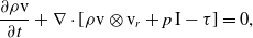 \begin{align}\frac{{\partial \rho {\textrm{v}}}}{{\partial t}} + \nabla \cdot [\rho {\textrm{v}} \otimes {{\textrm{v}}_r} + p\,{\textrm{I}} - \tau ] = 0,\end{align}
 \begin{align}\frac{{\partial \rho E}}{{\partial t}} + \nabla \cdot [\rho {{\textrm{v}}_r}E + p\,{\textrm{v}} - \tau \cdot {\textrm{v}} - \kappa \nabla T] = 0,\end{align}
where
 $\tau $
is the stress tensor,
$\tau $
is the stress tensor,
 $p$
is pressure,
$p$
is pressure,
 ${\textrm{I}}$
is the identity matrix,
${\textrm{I}}$
is the identity matrix,
 $\kappa $
is themal conductivity and
$\kappa $
is themal conductivity and
 $T$
is temperature. The total internal energy
$T$
is temperature. The total internal energy
 $E$
is defined as
$E$
is defined as
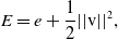 \begin{align}E = e + \frac{1}{2}||{\textrm{v}}{||^2},\end{align}
where
 $e$
is the internal energy. It can be shown that
$e$
is the internal energy. It can be shown that
 $\rho $
,
$\rho $
,
 $p$
,
$p$
,
 $T$
and
$T$
and
 $e$
are invariant, and investigation of the constitutive relations shows that
$e$
are invariant, and investigation of the constitutive relations shows that
 $\tau $
is invariant. Then in
$\tau $
is invariant. Then in
 ${\Sigma ^{\prime}}$
for linear acceleration
${\Sigma ^{\prime}}$
for linear acceleration
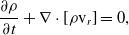 \begin{align}\frac{{\partial \rho }}{{\partial t}} + \nabla \cdot [\rho {{\textrm{v}}_r}] = 0,\end{align}
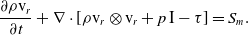 \begin{align}\frac{{\partial \rho {{\textrm{v}}_r}}}{{\partial t}} + \nabla \cdot [\rho {{\textrm{v}}_r} \otimes {{\textrm{v}}_r} + p\,{\textrm{I}} - \tau ] = {S_m}.\end{align}
It is appropriate to define a rothalpy
 ${E_r}$
:
${E_r}$
:
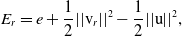 \begin{align}{E_r} = e + \frac{1}{2}||{{\textrm{v}}_r}{||^2} - \frac{1}{2}||{\textrm{u}}{||^2},\end{align}
which allows the transform of equation (5) into
 ${\Sigma ^{\prime}}$
to take the following convenient form
${\Sigma ^{\prime}}$
to take the following convenient form
 \begin{align}\frac{{\partial \rho {E_r}}}{{\partial t}} + \nabla \cdot [\rho {{\textrm{v}}_r}{E_r} + p\,{{\textrm{v}}_r} - \tau \cdot {{\textrm{v}}_r} - \kappa \nabla T] = {S_e},\end{align}
where the respective source terms [Reference Roohani19]
 ${S_m}$
and
${S_m}$
and
 ${S_e}$
are given in Section 2.2.2.
${S_e}$
are given in Section 2.2.2.
B Appendix
This appendix contains a total of five image sets to contrast steady state with acceleration and deceleration results for selected cone angles:
 $\theta $
= 20
$\theta $
= 20
 $^ \circ $
and 30
$^ \circ $
and 30
 $^ \circ $
, the MRF acceleration technique was used.
$^ \circ $
, the MRF acceleration technique was used.
8.1 Steady state and low transonic acceleration
Figure 13 contrasts the shoulder flow between steady state and 100g acceleration at flight Mach numbers 0.80, 0.85, and 0.90 for
 $\theta $
= 20
$\theta $
= 20
 $^ \circ $
.
$^ \circ $
.

Figure 13. Shoulder flow comparison between steady state and 100g acceleration for
 $\theta $
= 20
$\theta $
= 20
 $^ \circ $
at Mach numbers 0.80, 0.85 and 0.90. Top row: steady state, bottom row: low transonic acceleration. Flow direction read left to right and wave motion for the acceleration cases is left to right. Image sequence for this figure is left to right.
$^ \circ $
at Mach numbers 0.80, 0.85 and 0.90. Top row: steady state, bottom row: low transonic acceleration. Flow direction read left to right and wave motion for the acceleration cases is left to right. Image sequence for this figure is left to right.

Figure 14. Shoulder flow comparison between steady state and 100g acceleration for
 $\theta $
= 30
$\theta $
= 30
 $^ \circ $
at Mach numbers 0.90, 0.95 and 1.0. Top row: steady state, bottom row: low transonic acceleration. Flow direction is left to right and wave motion for the acceleration cases is left to right. Image sequence for this figure is left to right.
$^ \circ $
at Mach numbers 0.90, 0.95 and 1.0. Top row: steady state, bottom row: low transonic acceleration. Flow direction is left to right and wave motion for the acceleration cases is left to right. Image sequence for this figure is left to right.

Figure 15. Shoulder flow comparison between steady state and 100g deceleration for
 $\theta $
= 20
$\theta $
= 20
 $^ \circ $
at Mach numbers 0.92, 0.90 and 0.88. Top row: steady state, bottom row: low transonic deceleration. Flow direction is left to right and wave propagation is right to left. Image sequence for this figure is right to left. Single color bar is applicable per cone half-angle.
$^ \circ $
at Mach numbers 0.92, 0.90 and 0.88. Top row: steady state, bottom row: low transonic deceleration. Flow direction is left to right and wave propagation is right to left. Image sequence for this figure is right to left. Single color bar is applicable per cone half-angle.

Figure 16. Shoulder flow comparison between steady state and 100g deceleration for
 $\theta $
= 20
$\theta $
= 20
 $^ \circ $
at Mach numbers 0.75, 0.80 and 0.85. Top row: steady state, bottom row: low transonic deceleration. Flow direction is left to right and wave propagation is right to left. Image sequence for this figure is right to left.
$^ \circ $
at Mach numbers 0.75, 0.80 and 0.85. Top row: steady state, bottom row: low transonic deceleration. Flow direction is left to right and wave propagation is right to left. Image sequence for this figure is right to left.
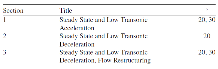
Figure 17. Shoulder flow comparison between steady state and 100g deceleration for
 $\theta $
= 30
$\theta $
= 30
 $^ \circ $
at Mach numbers 0.75, 0.80 and 0.85. Top row: steady state, bottom row: low transonic deceleration. Flow direction is left to right and wave propagation is right to left. Image sequence for this figure is right to left.
$^ \circ $
at Mach numbers 0.75, 0.80 and 0.85. Top row: steady state, bottom row: low transonic deceleration. Flow direction is left to right and wave propagation is right to left. Image sequence for this figure is right to left.
Figure 14 contrasts the shoulder flow between steady state and 100g acceleration at flight Mach numbers 0.90, 0.95, and 1.0 for
 $\theta $
= 30
$\theta $
= 30
 $^ \circ $
.
$^ \circ $
.
8.2 Steady state and low transonic deceleration
Figure 15 illustrates the absence of shock wave propagation upon the cone-cylinder with focus on the shoulder region for steady state flow in comparison to 100g deceleration at flight Mach numbers 0.92, 0.90, and 0.88 for
 $\theta $
= 20
$\theta $
= 20
 $^ \circ $
only.
$^ \circ $
only.
Figure 18. Relative Mach number contours during low transonic deceleration,
 ${a_0}$
= 100g, descending order for
${a_0}$
= 100g, descending order for
 $0.85 \lt {\textrm{M}} \lt 0.95$
, case #2 and
$0.85 \lt {\textrm{M}} \lt 0.95$
, case #2 and
 $\theta $
= 10
$\theta $
= 10
 $^ \circ $
, 20
$^ \circ $
, 20
 $^ \circ $
, 30
$^ \circ $
, 30
 $^ \circ $
. Flow direction is left to right and wave propagation is right to left. Image sequence in time for this figure is right to left.
$^ \circ $
. Flow direction is left to right and wave propagation is right to left. Image sequence in time for this figure is right to left.
8.3 Steady state and low transonic deceleration (Flow restructuring)
Figure 16 compares the shoulder flow between steady and 100g deceleration at flight Mach numbers 0.75, 0.80, and 0.85 for
 $\theta $
= 20
$\theta $
= 20
 $^ \circ $
.
$^ \circ $
.


 Open access