1. Introduction
In the spatial Johnson–Mehl growth model, seeds arrive at random times
![]() $t_i$
,
$t_i$
,
![]() $i \in \mathbb{N}$
, at random locations
$i \in \mathbb{N}$
, at random locations
![]() $x_i$
,
$x_i$
,
![]() $i \in \mathbb{N}$
, in
$i \in \mathbb{N}$
, in
![]() $\mathbb{R}^d$
, according to a Poisson process
$\mathbb{R}^d$
, according to a Poisson process
![]() $(x_i,t_i)_{i \in \mathbb{N}}$
on
$(x_i,t_i)_{i \in \mathbb{N}}$
on
![]() $\mathbb{R}^d \times \mathbb{R}_+$
, where
$\mathbb{R}^d \times \mathbb{R}_+$
, where
![]() $\mathbb{R}_+\,:\!=\,[0,\infty)$
. Once a seed is born at time t, it begins to form a cell by growing radially in all directions at a constant speed
$\mathbb{R}_+\,:\!=\,[0,\infty)$
. Once a seed is born at time t, it begins to form a cell by growing radially in all directions at a constant speed
![]() $v\geq 0$
, so that by time
$v\geq 0$
, so that by time
![]() $t^{\prime}$
it occupies the ball of radius
$t^{\prime}$
it occupies the ball of radius
![]() $v(t'-t)$
. The parts of the space claimed by the seeds form the so-called Johnson–Mehl tessellation; see [Reference Chiu, Stoyan, Kendall and Mecke7] and [Reference Okabe, Boots, Sugihara and Chiu16]. This is a generalization of the classical Voronoi tessellation, which is obtained if all births occur simultaneously at time zero.
$v(t'-t)$
. The parts of the space claimed by the seeds form the so-called Johnson–Mehl tessellation; see [Reference Chiu, Stoyan, Kendall and Mecke7] and [Reference Okabe, Boots, Sugihara and Chiu16]. This is a generalization of the classical Voronoi tessellation, which is obtained if all births occur simultaneously at time zero.
The study of such birth–growth processes started with the work of Kolmogorov [Reference Kolmogorov11] to model crystal growth in two dimensions. Since then, this model has seen applications in various contexts, such as phase transition kinetics, polymers, ecological systems, and DNA replications, to name a few; see [Reference Bollobás and Riordan4, Reference Chiu, Stoyan, Kendall and Mecke7, Reference Okabe, Boots, Sugihara and Chiu16] and references therein. A central limit theorem for the Johnson–Mehl model with inhomogeneous arrivals of the seeds was obtained in [Reference Chiu and Quine5].
Variants of the classical spatial birth–growth model can be found, sometimes as a particular case of other models, in many papers. Among them, we mention [Reference Baryshnikov and Yukich2] and [Reference Penrose and Yukich17], where the birth–growth model appears as a particular case of a random sequential packing model, and [Reference Schreiber and Yukich20], which studied a variant of the model with non-uniform deterministic growth patterns. The main tools rely on the concept of stabilization by considering regions where the appearance of new seeds influences the functional of interest.
In this paper, we consider a generalization of the Johnson–Mehl model by introducing random growth speeds for the seeds. This gives rise to many interesting features in the model, most importantly, long-range interactions if the speed can take arbitrarily large values with positive probability. Therefore, the model with random speed is no longer stabilizing in the classical sense of [Reference Lachièze-Rey, Schulte and Yukich13] and [Reference Penrose and Yukich18], since distant points may influence the growth pattern if their speeds are sufficiently high. It should be noted that, even in the constant-speed setting, we substantially improve and extend limit theorems obtained in [Reference Chiu and Quine5].
We consider a birth–growth model, determined by a Poisson process
![]() $\eta$
in
$\eta$
in
![]() $\mathbb{X}\,:\!=\,\mathbb{R}^d\times\mathbb{R}_+\times\mathbb{R}_+$
with intensity measure
$\mathbb{X}\,:\!=\,\mathbb{R}^d\times\mathbb{R}_+\times\mathbb{R}_+$
with intensity measure
![]() $\mu\,:\!=\,\lambda\otimes\theta\otimes\nu$
, where
$\mu\,:\!=\,\lambda\otimes\theta\otimes\nu$
, where
![]() $\lambda$
is the Lebesgue measure on
$\lambda$
is the Lebesgue measure on
![]() $\mathbb{R}^d$
,
$\mathbb{R}^d$
,
![]() $\theta$
is a non-null locally finite measure on
$\theta$
is a non-null locally finite measure on
![]() $\mathbb{R}_+$
, and
$\mathbb{R}_+$
, and
![]() $\nu$
is a probability distribution on
$\nu$
is a probability distribution on
![]() $\mathbb{R}_+$
with
$\mathbb{R}_+$
with
![]() $\nu(\{0\})<1$
. Each point
$\nu(\{0\})<1$
. Each point
![]() ${\boldsymbol{x}}$
of this point process
${\boldsymbol{x}}$
of this point process
![]() $\eta$
has three components
$\eta$
has three components
![]() $(x,t_x,v_x)$
, where
$(x,t_x,v_x)$
, where
![]() $v_x \in \mathbb{R}_+$
denotes the random speed of a seed born at location
$v_x \in \mathbb{R}_+$
denotes the random speed of a seed born at location
![]() $x \in \mathbb{R}^d$
and whose growth commences at time
$x \in \mathbb{R}^d$
and whose growth commences at time
![]() $t_x\in \mathbb{R}_+$
. In a given point configuration, a point
$t_x\in \mathbb{R}_+$
. In a given point configuration, a point
![]() ${\boldsymbol{x}}\,:\!=\,(x,t_x,v_x)$
is said to be exposed if there is no other point
${\boldsymbol{x}}\,:\!=\,(x,t_x,v_x)$
is said to be exposed if there is no other point
![]() $(y,t_y,v_y)$
in the configuration with
$(y,t_y,v_y)$
in the configuration with
![]() $t_y <t_x$
and
$t_y <t_x$
and
![]() $\|x-y\| \le v_y(t_x-t_y)$
, where
$\|x-y\| \le v_y(t_x-t_y)$
, where
![]() $\|\cdot\|$
denotes the Euclidean norm. Notice that the event that a point
$\|\cdot\|$
denotes the Euclidean norm. Notice that the event that a point
![]() $(x,t_x,v_x)\in \eta$
is exposed depends only on the point configuration in the region
$(x,t_x,v_x)\in \eta$
is exposed depends only on the point configuration in the region
Namely,
![]() ${\boldsymbol{x}}$
is exposed if and only if
${\boldsymbol{x}}$
is exposed if and only if
![]() $\eta$
has no points (apart from
$\eta$
has no points (apart from
![]() ${\boldsymbol{x}}$
) in
${\boldsymbol{x}}$
) in
![]() $L_{x,t_x}$
.
$L_{x,t_x}$
.
The growth frontier of the model can be defined as the random field
This is an example of an extremal shot-noise process; see [Reference Heinrich and Molchanov10]. Its value at a point
![]() $y \in \mathbb{R}^d$
corresponds to a seed from
$y \in \mathbb{R}^d$
corresponds to a seed from
![]() $\eta$
whose growth region covers y first. It should be noted here that this covering seed need not be an exposed one. In other words, because of random speeds, it may happen that the cell grown from a non-exposed seed shades a subsequent seed which would be exposed otherwise. This excludes possible applications of our model with random growth speed to crystallisation, where a more natural model would be to not allow a non-exposed seed to affect any future seeds. But this creates a causal chain of influences that seems quite difficult to study with the currently known methods of stabilization for Gaussian approximation.
$\eta$
whose growth region covers y first. It should be noted here that this covering seed need not be an exposed one. In other words, because of random speeds, it may happen that the cell grown from a non-exposed seed shades a subsequent seed which would be exposed otherwise. This excludes possible applications of our model with random growth speed to crystallisation, where a more natural model would be to not allow a non-exposed seed to affect any future seeds. But this creates a causal chain of influences that seems quite difficult to study with the currently known methods of stabilization for Gaussian approximation.
Nonetheless, models such as ours are natural in telecommunication applications, with the speed playing the role of the weight or strength of a particular transmission node, where the growth frontier defined above can be used as a variant of the additive signal-to-interference model from [Reference Baccelli and Błaszczyszyn1, Chapter 5]. Furthermore, similar models can be applied in the ecological or epidemiological context, where a non-visible event influences appearances of others. Suppose we have a barren land and a drone/machine is planting seeds from a mixture of plant species at random times and random locations for reforestation. Each seed, after falling on the ground, starts growing a bush around it at a random speed depending on its species. If a new seed falls on a part of the ground that is already covered in bushes, it is still allowed to form its own bush; i.e., there is no exclusion. Now the number of exposed points in our model above translates to the number of seeds that start a bush on a then barren piece of land, rather than starting on a piece of ground already covered in bushes. This, in some sense, can explain the efficiency of the reforestation process, i.e., what fraction of the seeds were planted on barren land, in contrast to being planted on already existing bushes.
Given a measurable weight function
![]() $h\;:\;\mathbb{R}^d \times \mathbb{R}_+ \to \mathbb{R}_+$
, the main object of interest in this paper is the sum of h over the space–time coordinates
$h\;:\;\mathbb{R}^d \times \mathbb{R}_+ \to \mathbb{R}_+$
, the main object of interest in this paper is the sum of h over the space–time coordinates
![]() $(x,t_x)$
of the exposed points in
$(x,t_x)$
of the exposed points in
![]() $\eta$
. These can be defined as those points
$\eta$
. These can be defined as those points
![]() $(y,t_y)$
where the growth frontier defined at (1.2) has a local minimum (see Section 2 for a precise definition). Our aim is to provide sufficient conditions for Gaussian convergence of such sums. A standard approach for proving Gaussian convergence for such statistics relies on stabilization theory [Reference Baryshnikov and Yukich2, Reference Eichelsbacher, Raič and Schreiber8, Reference Penrose and Yukich17, Reference Schreiber and Yukich20]. While in the stabilization literature one commonly assumes that the so-called stabilization region is a ball around a given reference point, the region
$(y,t_y)$
where the growth frontier defined at (1.2) has a local minimum (see Section 2 for a precise definition). Our aim is to provide sufficient conditions for Gaussian convergence of such sums. A standard approach for proving Gaussian convergence for such statistics relies on stabilization theory [Reference Baryshnikov and Yukich2, Reference Eichelsbacher, Raič and Schreiber8, Reference Penrose and Yukich17, Reference Schreiber and Yukich20]. While in the stabilization literature one commonly assumes that the so-called stabilization region is a ball around a given reference point, the region
![]() $L_{x,t_x}$
is unbounded and it seems that it is not expressible as a ball around
$L_{x,t_x}$
is unbounded and it seems that it is not expressible as a ball around
![]() ${\boldsymbol{x}}$
in some different metric. Moreover, our stabilization region is set to be empty if
${\boldsymbol{x}}$
in some different metric. Moreover, our stabilization region is set to be empty if
![]() ${\boldsymbol{x}}$
is not exposed.
${\boldsymbol{x}}$
is not exposed.
The main challenge when working with random unbounded speeds of growth is that there are possibly very long-range interactions between seeds. This makes the use of balls as stabilization regions vastly suboptimal and necessitates the use of regions of a more general shape. In particular, we only assume that the random growth speed in our model has finite moment of order 7d (see the assumption (C) in Section 2), and this allows for some power-tailed distributions for the speed.
The recent work [Reference Bhattacharjee and Molchanov3] introduced a new notion of region-stabilization which allows for more general regions than balls and, building on the seminal work [Reference Last, Peccati and Schulte14], provides bounds on the rate of Gaussian convergence for certain sums of region-stabilizing score functions. We will utilize this to derive bounds on the Wasserstein and Kolmogorov distances, defined below, between a suitably normalized sum of weights and the standard Gaussian distribution. For real-valued random variables X and Y, the Wasserstein distance between their distributions is given by
where
![]() $\operatorname{Lip}_1$
denotes the class of all Lipschitz functions
$\operatorname{Lip}_1$
denotes the class of all Lipschitz functions
![]() $f\;:\; \mathbb{R} \to \mathbb{R}$
with Lipschitz constant at most one. The Kolmogorov distance between the distributions is given by
$f\;:\; \mathbb{R} \to \mathbb{R}$
with Lipschitz constant at most one. The Kolmogorov distance between the distributions is given by
The rest of the paper is organized as follows. In Section 2, we describe the model and state our main results. In Section 3, we prove a result providing necessary upper and lower bounds for the variance of our statistic of interest. Section 4 presents the proofs of our quantitative bounds.
2. Model and main results
Recall that we work in the space
![]() $\mathbb{X}\,:\!=\,\mathbb{R}^d\times\mathbb{R}_+\times\mathbb{R}_+$
,
$\mathbb{X}\,:\!=\,\mathbb{R}^d\times\mathbb{R}_+\times\mathbb{R}_+$
,
![]() $d \in \mathbb{N}$
, with the Borel
$d \in \mathbb{N}$
, with the Borel
![]() $\sigma$
-algebra. The points from
$\sigma$
-algebra. The points from
![]() $\mathbb{X}$
are written as
$\mathbb{X}$
are written as
![]() ${\boldsymbol{x}}\,:\!=\,(x,t_x,v_x)$
, so that
${\boldsymbol{x}}\,:\!=\,(x,t_x,v_x)$
, so that
![]() ${\boldsymbol{x}}$
designates a seed born in position x at time
${\boldsymbol{x}}$
designates a seed born in position x at time
![]() $t_x$
, which then grows radially in all directions with speed
$t_x$
, which then grows radially in all directions with speed
![]() $v_x$
. For
$v_x$
. For
![]() ${\boldsymbol{x}}\in \mathbb{X}$
, the set
${\boldsymbol{x}}\in \mathbb{X}$
, the set
is the growth region of the seed
![]() ${\boldsymbol{x}}$
. Denote by
${\boldsymbol{x}}$
. Denote by
![]() $\textbf{N}$
the family of
$\textbf{N}$
the family of
![]() $\sigma$
-finite counting measures
$\sigma$
-finite counting measures
![]() $\mathcal{M}$
on
$\mathcal{M}$
on
![]() $\mathbb{X}$
equipped with the smallest
$\mathbb{X}$
equipped with the smallest
![]() $\sigma$
-algebra
$\sigma$
-algebra
![]() $\mathscr{N}\ $
such that the maps
$\mathscr{N}\ $
such that the maps
![]() $\mathcal{M} \mapsto \mathcal{M}(A)$
are measurable for all Borel A. We write
$\mathcal{M} \mapsto \mathcal{M}(A)$
are measurable for all Borel A. We write
![]() ${\boldsymbol{x}}\in\mathcal{M}$
if
${\boldsymbol{x}}\in\mathcal{M}$
if
![]() $\mathcal{M}(\{{\boldsymbol{x}}\})\geq 1$
. For
$\mathcal{M}(\{{\boldsymbol{x}}\})\geq 1$
. For
![]() $\mathcal{M} \in \textbf{N}$
, a point
$\mathcal{M} \in \textbf{N}$
, a point
![]() ${\boldsymbol{x}} \in \mathcal{M}$
is said to be exposed in
${\boldsymbol{x}} \in \mathcal{M}$
is said to be exposed in
![]() $\mathcal{M}$
if it does not belong to the growth region of any other point
$\mathcal{M}$
if it does not belong to the growth region of any other point
![]() ${\boldsymbol{y}}\in\mathcal{M}$
,
${\boldsymbol{y}}\in\mathcal{M}$
,
![]() ${\boldsymbol{y}} \neq {\boldsymbol{x}}$
. Note that the property of being exposed is not influenced by the speed component of
${\boldsymbol{y}} \neq {\boldsymbol{x}}$
. Note that the property of being exposed is not influenced by the speed component of
![]() ${\boldsymbol{x}}$
.
${\boldsymbol{x}}$
.
The influence set
![]() $L_{\boldsymbol{x}}=L_{x,t_x}$
,
$L_{\boldsymbol{x}}=L_{x,t_x}$
,
![]() ${\boldsymbol{x}} \in \mathbb{X}$
, defined at (1.1), is exactly the set of points that were born before time
${\boldsymbol{x}} \in \mathbb{X}$
, defined at (1.1), is exactly the set of points that were born before time
![]() $t_x$
and which at time
$t_x$
and which at time
![]() $t_x$
occupy a region that covers the location x, thereby shading it. Note that
$t_x$
occupy a region that covers the location x, thereby shading it. Note that
![]() ${\boldsymbol{y}}\in L_{\boldsymbol{x}}$
if and only if
${\boldsymbol{y}}\in L_{\boldsymbol{x}}$
if and only if
![]() ${\boldsymbol{x}}\in G_{\boldsymbol{y}}$
. Clearly, a point
${\boldsymbol{x}}\in G_{\boldsymbol{y}}$
. Clearly, a point
![]() ${\boldsymbol{x}}\in\mathcal{M}$
is exposed in
${\boldsymbol{x}}\in\mathcal{M}$
is exposed in
![]() $\mathcal{M}$
if and only if
$\mathcal{M}$
if and only if
![]() $\mathcal{M} (L_{\boldsymbol{x}}\setminus\{x\})=0$
. We write
$\mathcal{M} (L_{\boldsymbol{x}}\setminus\{x\})=0$
. We write
![]() $(y,t_y,v_y)\preceq (x,t_x)$
or
$(y,t_y,v_y)\preceq (x,t_x)$
or
![]() ${\boldsymbol{y}} \preceq {\boldsymbol{x}}$
if
${\boldsymbol{y}} \preceq {\boldsymbol{x}}$
if
![]() ${\boldsymbol{y}}\in L_{x,t_x}$
(recall that the speed component of
${\boldsymbol{y}}\in L_{x,t_x}$
(recall that the speed component of
![]() ${\boldsymbol{x}}$
is irrelevant in such a relation), and so
${\boldsymbol{x}}$
is irrelevant in such a relation), and so
![]() ${\boldsymbol{x}}$
is not an exposed point with respect to
${\boldsymbol{x}}$
is not an exposed point with respect to
![]() $\delta_{{\boldsymbol{y}}}$
, where
$\delta_{{\boldsymbol{y}}}$
, where
![]() $\delta_{{\boldsymbol{y}}}$
denotes the Dirac measure at
$\delta_{{\boldsymbol{y}}}$
denotes the Dirac measure at
![]() ${\boldsymbol{y}}$
.
${\boldsymbol{y}}$
.
For
![]() $\mathcal{M} \in \textbf{N}$
and
$\mathcal{M} \in \textbf{N}$
and
![]() ${\boldsymbol{x}} \in \mathcal{M}$
, define
${\boldsymbol{x}} \in \mathcal{M}$
, define
A generic way to construct an additive functional on the exposed points is to consider the sum of weights of these points, where each exposed point
![]() ${\boldsymbol{x}}$
contributes a weight
${\boldsymbol{x}}$
contributes a weight
![]() $h({\boldsymbol{x}})$
for some measurable
$h({\boldsymbol{x}})$
for some measurable
![]() $h\;: \; \mathbb{X} \to \mathbb{R}_+$
. In the following we consider weight functions
$h\;: \; \mathbb{X} \to \mathbb{R}_+$
. In the following we consider weight functions
![]() $h({\boldsymbol{x}})$
which are products of two measurable functions
$h({\boldsymbol{x}})$
which are products of two measurable functions
![]() $h_1\; :\;\mathbb {R}^d \to \mathbb{R}_+$
and
$h_1\; :\;\mathbb {R}^d \to \mathbb{R}_+$
and
![]() $h_2\;: \; \mathbb{R}_+ \to \mathbb{R}_+$
of the locations and birth times, respectively, of the exposed points. In particular, we let
$h_2\;: \; \mathbb{R}_+ \to \mathbb{R}_+$
of the locations and birth times, respectively, of the exposed points. In particular, we let
![]() $h_1(x) = \unicode{x1d7d9}_W(x)=\unicode{x1d7d9}\{x \in W\}$
for a window
$h_1(x) = \unicode{x1d7d9}_W(x)=\unicode{x1d7d9}\{x \in W\}$
for a window
![]() $W \subset \mathbb{R}^d$
, and
$W \subset \mathbb{R}^d$
, and
![]() $h_2(t) = \unicode{x1d7d9}\{t \le a\}$
for
$h_2(t) = \unicode{x1d7d9}\{t \le a\}$
for
![]() $a \in (0,\infty)$
. Then
$a \in (0,\infty)$
. Then
is the number of exposed points from
![]() $\mathcal{M}$
located in W and born before time a. Note here that when we add a new point
$\mathcal{M}$
located in W and born before time a. Note here that when we add a new point
![]() ${\boldsymbol{y}}=(y,t_y,v_y) \in \mathbb{R}^d \times \mathbb{R}_+ \times \mathbb{R}_+$
to a configuration
${\boldsymbol{y}}=(y,t_y,v_y) \in \mathbb{R}^d \times \mathbb{R}_+ \times \mathbb{R}_+$
to a configuration
![]() $\mathcal{M} \in \textbf{N}$
not containing it, the change in the value of F is not a function of only
$\mathcal{M} \in \textbf{N}$
not containing it, the change in the value of F is not a function of only
![]() ${\boldsymbol{y}}$
and some local neighborhood of it, but rather depends on points in the configuration that might be very far away. Indeed, for
${\boldsymbol{y}}$
and some local neighborhood of it, but rather depends on points in the configuration that might be very far away. Indeed, for
![]() ${\boldsymbol{y}} \notin \mathcal{M}$
we have
${\boldsymbol{y}} \notin \mathcal{M}$
we have
that is, F may increase by one when
![]() ${\boldsymbol{y}}$
is exposed in
${\boldsymbol{y}}$
is exposed in
![]() $\mathcal{M} + \delta_{{\boldsymbol{y}}}$
, while simultaneously, any point
$\mathcal{M} + \delta_{{\boldsymbol{y}}}$
, while simultaneously, any point
![]() ${\boldsymbol{x}}\in\mathcal{M}$
which was previously exposed in
${\boldsymbol{x}}\in\mathcal{M}$
which was previously exposed in
![]() $\mathcal{M}$
may not be so anymore after the addition of
$\mathcal{M}$
may not be so anymore after the addition of
![]() ${\boldsymbol{y}}$
, if it happens to fall in the influence set
${\boldsymbol{y}}$
, if it happens to fall in the influence set
![]() $L_{(y,t_y)}$
of
$L_{(y,t_y)}$
of
![]() ${\boldsymbol{y}}$
. This necessitates the use of region-stabilization.
${\boldsymbol{y}}$
. This necessitates the use of region-stabilization.
Recall that
![]() $\eta$
is a Poisson process in
$\eta$
is a Poisson process in
![]() $\mathbb{X}$
with intensity measure
$\mathbb{X}$
with intensity measure
![]() $\mu$
, being the product of the Lebesgue measure
$\mu$
, being the product of the Lebesgue measure
![]() $\lambda$
on
$\lambda$
on
![]() $\mathbb{R}^d$
, a non-null locally finite measure
$\mathbb{R}^d$
, a non-null locally finite measure
![]() $\theta$
on
$\theta$
on
![]() $\mathbb{R}_+$
, and a probability measure
$\mathbb{R}_+$
, and a probability measure
![]() $\nu$
on
$\nu$
on
![]() $\mathbb{R}_+$
with
$\mathbb{R}_+$
with
![]() $\nu(\{0\})<1$
. Note that
$\nu(\{0\})<1$
. Note that
![]() $\eta$
is a simple random counting measure. The main goal of this paper is to find sufficient conditions for a Gaussian convergence of
$\eta$
is a simple random counting measure. The main goal of this paper is to find sufficient conditions for a Gaussian convergence of
![]() $F\equiv F(\eta)$
as defined at (2.1). The functional
$F\equiv F(\eta)$
as defined at (2.1). The functional
![]() $F(\eta)$
is a region-stabilizing functional, in the sense of [Reference Bhattacharjee and Molchanov3], and can be represented as
$F(\eta)$
is a region-stabilizing functional, in the sense of [Reference Bhattacharjee and Molchanov3], and can be represented as
![]() $F(\eta)=\sum_{{\boldsymbol{x}} \in \eta} \xi({\boldsymbol{x}}, \eta)$
, where the score function
$F(\eta)=\sum_{{\boldsymbol{x}} \in \eta} \xi({\boldsymbol{x}}, \eta)$
, where the score function
![]() $\xi$
is given by
$\xi$
is given by
with the region of stabilization being
![]() $L_{x,t_x}$
when
$L_{x,t_x}$
when
![]() ${\boldsymbol{x}}$
is an exposed point (see Section 4 for more details). As a convention, let
${\boldsymbol{x}}$
is an exposed point (see Section 4 for more details). As a convention, let
![]() $\xi({\boldsymbol{x}},\mathcal{M})=0$
if
$\xi({\boldsymbol{x}},\mathcal{M})=0$
if
![]() $\mathcal{M}=0$
or if
$\mathcal{M}=0$
or if
![]() $x\notin\mathcal{M}$
. Theorem 2.1 in [Reference Bhattacharjee and Molchanov3] yields ready-to-use bounds on the Wasserstein and Kolmogorov distances between F, suitably normalized, and a standard Gaussian random variable N upon validating Equation (2.1) and the conditions (A1) and (A2) therein. We consistently follow the notation of [Reference Bhattacharjee and Molchanov3].
$x\notin\mathcal{M}$
. Theorem 2.1 in [Reference Bhattacharjee and Molchanov3] yields ready-to-use bounds on the Wasserstein and Kolmogorov distances between F, suitably normalized, and a standard Gaussian random variable N upon validating Equation (2.1) and the conditions (A1) and (A2) therein. We consistently follow the notation of [Reference Bhattacharjee and Molchanov3].
Now we are ready to state our main results. First, we list the necessary assumptions on our model. In the sequel, we drop the
![]() $\lambda$
in Lebesgue integrals and simply write
$\lambda$
in Lebesgue integrals and simply write
![]() ${\textrm{d}} x$
instead of
${\textrm{d}} x$
instead of
![]() $\lambda({\textrm{d}} x)$
. Our assumptions are as follows:
$\lambda({\textrm{d}} x)$
. Our assumptions are as follows:
-
(A) The window W is compact convex with non-empty interior.
-
(B) For all
 $x>0$
, where
 \begin{equation*} \int_0^\infty e^{-x \Lambda(t)} \, \theta({\textrm{d}} t)<\infty, \end{equation*}
(2.3)and
 \begin{equation} \Lambda(t)\,:\!=\,\omega_d\int_0^t (t-s)^d \theta({\textrm{d}} s) \end{equation}
 $\omega_d$
is the volume of the d-dimensional unit Euclidean ball.
-
(C) The moment of
 $\nu$
of order 7d is finite, i.e.,
 $\nu_{7d}<\infty$
, where
 \begin{equation*}\nu_{u}\,:\!=\,\int_0^\infty v^u \nu({\textrm{d}} v),\quad u\geq 0. \end{equation*}
Note that the function
![]() $\Lambda(t)$
given at (2.3) is, up to a constant, the measure of the influence set of any point
$\Lambda(t)$
given at (2.3) is, up to a constant, the measure of the influence set of any point
![]() ${\boldsymbol{x}} \in \mathbb{X}$
with time component
${\boldsymbol{x}} \in \mathbb{X}$
with time component
![]() $t_x=t$
(the measure of the influence set does not depend on the location and speed components of
$t_x=t$
(the measure of the influence set does not depend on the location and speed components of
![]() ${\boldsymbol{x}}$
). Indeed, the
${\boldsymbol{x}}$
). Indeed, the
![]() $\mu$
-content of
$\mu$
-content of
![]() $L_{x,t_x}$
is given by
$L_{x,t_x}$
is given by
 \begin{align} \mu(L_{x,t_x}) &=\int_{0}^\infty \int_0^{t_x} \int_{\mathbb{R}^d} \unicode{x1d7d9}_{y \in B_{v_y(t_x-t_y)}(x)} \,{\textrm{d}} y\,\theta({\textrm{d}} t_y)\nu({\textrm{d}} v_y)\\ & =\int_0^\infty \nu({\textrm{d}} v_y) \int_0^{t_x} \omega_d v_y^d(t_x-t_y)^d \theta({\textrm{d}} t_y)=\nu_{d} \Lambda(t_x),\end{align}
where
![]() $B_r(x)$
denotes the closed d-dimensional Euclidean ball of radius r centered at
$B_r(x)$
denotes the closed d-dimensional Euclidean ball of radius r centered at
![]() $x \in\mathbb{R}^d$
. In particular, if
$x \in\mathbb{R}^d$
. In particular, if
![]() $\theta$
is the Lebesgue measure on
$\theta$
is the Lebesgue measure on
![]() $\mathbb{R}_+$
, then
$\mathbb{R}_+$
, then
![]() $\Lambda(t)=\omega_d\,t^{d+1}/(d+1)$
.
$\Lambda(t)=\omega_d\,t^{d+1}/(d+1)$
.
The following theorem is our first main result. We denote by
![]() $(V_j(W))_{0 \le j \le d }$
the intrinsic volumes of W (see [Reference Schneider19, Section 4.1]), and let
$(V_j(W))_{0 \le j \le d }$
the intrinsic volumes of W (see [Reference Schneider19, Section 4.1]), and let
Theorem 2.1. Let
![]() $\eta$
be a Poisson process on
$\eta$
be a Poisson process on
![]() $\mathbb{X}$
with intensity measure
$\mathbb{X}$
with intensity measure
![]() $\mu$
as above, such that the assumptions (A)–(C) hold. Then, for
$\mu$
as above, such that the assumptions (A)–(C) hold. Then, for
![]() $F\,:\!=\,F(\eta)$
as in (2.1) with
$F\,:\!=\,F(\eta)$
as in (2.1) with
![]() $a \in (0,\infty)$
,
$a \in (0,\infty)$
,
 \begin{equation*} d_{\textrm{W}}\left(\frac{F - \mathbb{E} F}{\sqrt{\textrm{Var}\, F}},N\right) \le C \Bigg[\frac{\sqrt{V(W)}}{\textrm{Var}\, F} +\frac{V(W)}{(\textrm{Var}\, F)^{3/2}}\Bigg] \end{equation*}
and
 \begin{equation*} d_{\textrm{K}}\left(\frac{F - \mathbb{E} F}{\sqrt{\textrm{Var}\, F}},N\right) \le C \Bigg[\frac{\sqrt{V(W)}}{\textrm{Var}\, F}\\ +\frac{V(W)}{(\textrm{Var}\, F)^{3/2}} +\frac{V(W)^{5/4} + V(W)^{3/2}}{(\textrm{Var}\, F)^{2}}\Bigg] \end{equation*}
for a constant
![]() $C \in (0,\infty)$
which depends on a, d, the first 7d moments of
$C \in (0,\infty)$
which depends on a, d, the first 7d moments of
![]() $\nu$
, and
$\nu$
, and
![]() $\theta$
.
$\theta$
.
To derive a quantitative central limit theorem from Theorem 2.1, a lower bound on the variance is needed. The following proposition provides general lower and upper bounds on the variance, which are then specialized for measures on
![]() $\mathbb{R}_+$
given by
$\mathbb{R}_+$
given by
In the following,
![]() $t_1 \wedge t_2$
denotes
$t_1 \wedge t_2$
denotes
![]() $\min\{t_1,t_2\}$
for
$\min\{t_1,t_2\}$
for
![]() $t_1, t_2 \in \mathbb{R}$
. For
$t_1, t_2 \in \mathbb{R}$
. For
![]() $a \in (0,\infty)$
and
$a \in (0,\infty)$
and
![]() $\tau>-1$
, define the function
$\tau>-1$
, define the function
where
![]() $\gamma(p,z)\,:\!=\,\int_0^z t^{p-1}e^{-t}{\textrm{d}} t $
is the lower incomplete gamma function.
$\gamma(p,z)\,:\!=\,\int_0^z t^{p-1}e^{-t}{\textrm{d}} t $
is the lower incomplete gamma function.
Proposition 2.1. Let the assumptions (A)–(C) be in force. For a Poisson process
![]() $\eta$
with intensity measure
$\eta$
with intensity measure
![]() $\mu$
as above and
$\mu$
as above and
![]() $F\,:\!=\,F(\eta)$
as in (2.1),
$F\,:\!=\,F(\eta)$
as in (2.1),
 \begin{equation} \frac{\textrm{Var}(F)}{\lambda(W)} \ge \Bigg[\int_{0}^a w(t) \theta({\textrm{d}} t) - 2 \omega_d \nu_{d} \int_0^a \int_0^{t} (t-s)^d w(s) w(t) \theta({\textrm{d}} s) \theta({\textrm{d}} t)\Bigg] \end{equation}
and
 \begin{multline} \frac{\textrm{Var}(F)}{\lambda(W)} \le \Bigg[2 \int_{0}^a w(t)^{1/2} \theta({\textrm{d}} t)\\ \quad + \omega_d^2 \nu_{2d} \int_{[0,a]^2} \int_{0}^{t_1 \wedge t_2} (t_1-s)^d (t_2-s)^d w(t_1)^{1/2} w(t_2)^{1/2} \theta({\textrm{d}} s) \theta^2({\textrm{d}}(t_1,t_2))\Bigg], \end{multline}
where
If
![]() $\theta$
is given by (2.5), then
$\theta$
is given by (2.5), then
for constants
![]() $C_1, C_1', C_2$
depending on the dimension d and
$C_1, C_1', C_2$
depending on the dimension d and
![]() $\tau$
, and
$\tau$
, and
![]() $C_1,C_2>0$
.
$C_1,C_2>0$
.
We remark here that the lower bound in (2.10) is useful only when
![]() $\tau \le d-1$
. We believe that a positive lower bound still exists when
$\tau \le d-1$
. We believe that a positive lower bound still exists when
![]() $\tau>d-1$
, even though our arguments in general do not apply for such
$\tau>d-1$
, even though our arguments in general do not apply for such
![]() $\tau$
.
$\tau$
.
In the case of a deterministic speed v, Proposition 2.1 provides an explicit condition on
![]() $\theta$
ensuring that the variance scales like the volume of the observation window in the classical Johnson–Mehl growth model. The problem of finding such a condition, explicitly formulated in [Reference Chiu and Quine6, p. 754], arose in [Reference Chiu and Quine5], where asymptotic normality for the number of exposed seeds in a region, as the volume of the region approaches infinity, is obtained under the assumption that the variance scales properly. This was by then only shown numerically for the case when
$\theta$
ensuring that the variance scales like the volume of the observation window in the classical Johnson–Mehl growth model. The problem of finding such a condition, explicitly formulated in [Reference Chiu and Quine6, p. 754], arose in [Reference Chiu and Quine5], where asymptotic normality for the number of exposed seeds in a region, as the volume of the region approaches infinity, is obtained under the assumption that the variance scales properly. This was by then only shown numerically for the case when
![]() $\theta$
is the Lebesgue measure and
$\theta$
is the Lebesgue measure and
![]() $d=1,2,3,4$
. Subsequent papers [Reference Penrose and Yukich17, Reference Schreiber and Yukich20] derived the variance scaling for
$d=1,2,3,4$
. Subsequent papers [Reference Penrose and Yukich17, Reference Schreiber and Yukich20] derived the variance scaling for
![]() $\theta$
being the Lebesgue measure and some generalizations of it, but in a slightly different formulation of the model, in which seeds that do not appear in the observation window are automatically rejected and cannot influence the growth pattern in the region W.
$\theta$
being the Lebesgue measure and some generalizations of it, but in a slightly different formulation of the model, in which seeds that do not appear in the observation window are automatically rejected and cannot influence the growth pattern in the region W.
It should be noted that it might also be possible to use [Reference Lachièze-Rey12, Theorem 1.2] to obtain a quantitative central limit theorem and variance asymptotics for statistics of the exposed points in a domain W which is the union of unit cubes around a subset of points in
![]() $\mathbb{Z}^d$
. For this, one would need to check Assumption 1.1 from the cited paper, which ensures non-degeneracy of the variance, and a moment condition in the form of Equation (1.10) therein. It seems to us that checking Assumption 1.1 may be a challenging task and would involve further assumptions on the model, such as the one we also need in our Proposition 2.1. Controls on the long-range interactions would also be necessary to check [Reference Lachièze-Rey12, Equation (1.10)]. Thus, while this might indeed yield results similar to ours, the goal of the present work is to highlight the application of region-stabilization in this context, which in general is of a different nature from the methods in [Reference Lachièze-Rey12]. For example, the approach in [Reference Lachièze-Rey12] does not apply for Pareto-minimal points in a hypercube considered in [Reference Bhattacharjee and Molchanov3], since there is no polynomial decay in long-range interactions, while region-stabilization yields optimal rates for the Gaussian convergence.
$\mathbb{Z}^d$
. For this, one would need to check Assumption 1.1 from the cited paper, which ensures non-degeneracy of the variance, and a moment condition in the form of Equation (1.10) therein. It seems to us that checking Assumption 1.1 may be a challenging task and would involve further assumptions on the model, such as the one we also need in our Proposition 2.1. Controls on the long-range interactions would also be necessary to check [Reference Lachièze-Rey12, Equation (1.10)]. Thus, while this might indeed yield results similar to ours, the goal of the present work is to highlight the application of region-stabilization in this context, which in general is of a different nature from the methods in [Reference Lachièze-Rey12]. For example, the approach in [Reference Lachièze-Rey12] does not apply for Pareto-minimal points in a hypercube considered in [Reference Bhattacharjee and Molchanov3], since there is no polynomial decay in long-range interactions, while region-stabilization yields optimal rates for the Gaussian convergence.
The bounds in Theorem 2.1 can be specified under two different scenarios. When considering a sequence of weight functions, under suitable conditions Theorem 2.1 provides a quantitative central limit theorem for the corresponding functionals
![]() $(F_n)_{n \in \mathbb{N}}$
. Keeping all other quantities fixed with respect to n, consider the sequence of non-negative location-weight functions on
$(F_n)_{n \in \mathbb{N}}$
. Keeping all other quantities fixed with respect to n, consider the sequence of non-negative location-weight functions on
![]() $\mathbb{R}^d$
given by
$\mathbb{R}^d$
given by
![]() $h_{1,n} = \unicode{x1d7d9}_{n^{1/d} W}$
for a fixed convex body
$h_{1,n} = \unicode{x1d7d9}_{n^{1/d} W}$
for a fixed convex body
![]() $W \subset \mathbb{R}^d$
satisfying (A). In view of Proposition 2.1, this provides the following quantitative central limit theorem.
$W \subset \mathbb{R}^d$
satisfying (A). In view of Proposition 2.1, this provides the following quantitative central limit theorem.
Theorem 2.2. Let the assumptions (A)–(C) be in force. For
![]() $n \in \mathbb{N}$
and
$n \in \mathbb{N}$
and
![]() $\eta$
as in Theorem 2.1, let
$\eta$
as in Theorem 2.1, let
![]() $F_n\,:\!=\,F_n(\eta)$
, where
$F_n\,:\!=\,F_n(\eta)$
, where
![]() $F_n$
is defined as in (2.1) with a independent of n and
$F_n$
is defined as in (2.1) with a independent of n and
![]() $h_1=h_{1,n} = \unicode{x1d7d9}_{n^{1/d}W}$
. Assume that
$h_1=h_{1,n} = \unicode{x1d7d9}_{n^{1/d}W}$
. Assume that
![]() $\theta$
and
$\theta$
and
![]() $\nu$
satisfy
$\nu$
satisfy
where w(t) is given at (2.9). Then there exists a constant
![]() $C \in (0,\infty)$
, depending on a, d, the first 7d moments of
$C \in (0,\infty)$
, depending on a, d, the first 7d moments of
![]() $\nu$
,
$\nu$
,
![]() $\theta$
, and W, such that
$\theta$
, and W, such that
for all
![]() $n\in\mathbb{N}$
. In particular, (2.11) is satisfied for
$n\in\mathbb{N}$
. In particular, (2.11) is satisfied for
![]() $\theta$
given at (2.5) with
$\theta$
given at (2.5) with
![]() $\tau \in ({-}1,d-1]$
.
$\tau \in ({-}1,d-1]$
.
Furthermore, the bound on the Kolmogorov distance is of optimal order; i.e., when (2.11) holds, there exists a constant
![]() $0 < C' \le C$
depending only on a, d, the first 2d moments of
$0 < C' \le C$
depending only on a, d, the first 2d moments of
![]() $\nu$
,
$\nu$
,
![]() $\theta$
, and W, such that
$\theta$
, and W, such that
When (2.11) is satisfied, Theorem 2.2 yields a central limit theorem for the number of exposed seeds born before time
![]() $a\in (0,\infty)$
, with rate of convergence of order
$a\in (0,\infty)$
, with rate of convergence of order
![]() $n^{-1/2}$
. This extends the central limit theorem for the number of exposed seeds from [Reference Chiu and Quine5] in several directions: the model is generalized to random growth speeds, there is no constraint of any kind on the shape of the window W except convexity, and a logarithmic factor is removed from the rate of convergence.
$n^{-1/2}$
. This extends the central limit theorem for the number of exposed seeds from [Reference Chiu and Quine5] in several directions: the model is generalized to random growth speeds, there is no constraint of any kind on the shape of the window W except convexity, and a logarithmic factor is removed from the rate of convergence.
In a different scenario, if
![]() $\theta$
has a power-law density (2.5) with
$\theta$
has a power-law density (2.5) with
![]() $\tau \in ({-}1,d-1]$
, it is possible to explicitly specify the dependence of the bound in Theorem 2.1 on the moments of
$\tau \in ({-}1,d-1]$
, it is possible to explicitly specify the dependence of the bound in Theorem 2.1 on the moments of
![]() $\nu$
, as stated in the following result. Note that for the above choice of
$\nu$
, as stated in the following result. Note that for the above choice of
![]() $\theta$
, the assumption (B) is trivially satisfied. Define
$\theta$
, the assumption (B) is trivially satisfied. Define
 \begin{align}V_\nu(W)\,:\!=\,\sum_{i=0}^d V_{d-i}(W) \nu_{d+i},\end{align}
which is the sum of the intrinsic volumes of W weighted by the moments of the speed.
Theorem 2.3. Let the assumptions (A) and (C) be in force. For
![]() $\theta$
given at (2.5) with
$\theta$
given at (2.5) with
![]() $\tau \in ({-}1,$
$\tau \in ({-}1,$
![]() $d-1]$
, consider
$d-1]$
, consider
![]() $F=F(\eta)$
, where
$F=F(\eta)$
, where
![]() $\eta$
is as in Theorem 2.1 and F is defined as in (2.1) with
$\eta$
is as in Theorem 2.1 and F is defined as in (2.1) with
![]() $a \in (0,\infty)$
. Then there exists a constant
$a \in (0,\infty)$
. Then there exists a constant
![]() $C \in (0,\infty)$
, depending only on d and
$C \in (0,\infty)$
, depending only on d and
![]() $\tau$
, such that
$\tau$
, such that
 \begin{equation*} d_{\textrm{W}}\left(\frac{F - \mathbb{E} F}{\sqrt{\textrm{Var}\, F}},N\right)\\ \leq C (1+a^d) \left(1+\nu_{7d}\nu_{d}^{-7}\right)^{2} \Bigg[ \frac {\nu_{d}^{-\frac{1}{2}\left(\frac{\tau+1}{d+\tau+1}+1\right)} \sqrt{V_\nu(W)}}{l_{a,\tau}(\nu_d) \lambda(W)} + \frac{\nu_{d}^{-\frac{\tau+1}{d+\tau+1}-1} V_\nu(W)} {l_{a,\tau}(\nu_d)^{3/2}\lambda(W)^{3/2}} \Bigg]\,, \end{equation*}
and
 \begin{equation*} d_{\textrm{K}}\left(\frac{F - \mathbb{E} F}{\sqrt{\textrm{Var}\, F}},N\right) \leq C (1+a^d)^{3/2} \left(1+\nu_{7d}\nu_{d}^{-7}\right)^{2} \Bigg[ \frac {\nu_{d}^{-\frac{1}{2}\left(\frac{\tau+1}{d+\tau+1}+1\right)} \sqrt{V_\nu(W)}}{l_{a,\tau}(\nu_d) \lambda(W)} \\ + \frac{\nu_{d}^{-\frac{\tau+1}{d+\tau+1}-1} V_\nu(W)} {l_{a,\tau}(\nu_d)^{3/2}\lambda(W)^{3/2}} + \frac {\nu_{d}^{-\frac{5}{4}\left(\frac{\tau+1}{d+\tau+1}+1\right)}V_\nu(W)^{5/4} + \nu_{d}^{-\frac{3}{2}\left(\frac{\tau+1}{d+\tau+1}+1\right)} V_\nu(W)^{3/2}} {l_{a,\tau}(\nu_d)^2 \lambda(W)^{2}} \Bigg], \end{equation*}
where
![]() $l_{a,\tau}$
is defined at (2.6).
$l_{a,\tau}$
is defined at (2.6).
Note that our results for the number of exposed points can also be interpreted as quantitative central limit theorems for the number of local minima of the growth frontier, which is of independent interest. As an application of Theorem 2.3, we consider the case when the intensity of the underlying point process grows to infinity. The quantitative central limit theorem for this case is contained in the following result.
Corollary 2.1. Let the assumptions (A) and (C) be in force. Consider
![]() $F(\eta_s)$
defined at (2.1) with
$F(\eta_s)$
defined at (2.1) with
![]() $a \in (0,\infty)$
, evaluated at the Poisson process
$a \in (0,\infty)$
, evaluated at the Poisson process
![]() $\eta_s$
with intensity
$\eta_s$
with intensity
![]() $s\lambda\otimes\theta\otimes\nu$
for
$s\lambda\otimes\theta\otimes\nu$
for
![]() $s \ge 1$
and
$s \ge 1$
and
![]() $\theta$
given at (2.5) with
$\theta$
given at (2.5) with
![]() $\tau \in ({-}1,d-1]$
. Then there exists a finite constant
$\tau \in ({-}1,d-1]$
. Then there exists a finite constant
![]() $C \in (0,\infty)$
depending only on W, d, a,
$C \in (0,\infty)$
depending only on W, d, a,
![]() $\tau$
,
$\tau$
,
![]() $\nu_{d}$
, and
$\nu_{d}$
, and
![]() $\nu_{7d}$
, such that, for all
$\nu_{7d}$
, such that, for all
![]() $s\ge 1$
,
$s\ge 1$
,
Furthermore, the bound on the Kolmogorov distance is of optimal order.
3. Variance estimation
In this section, we estimate the mean and variance of the statistic F, thus providing a proof of Proposition 2.1. Recall the weight function
![]() $h({\boldsymbol{x}})\,:\!=\,h_1(x) h_2(t_x)$
, where
$h({\boldsymbol{x}})\,:\!=\,h_1(x) h_2(t_x)$
, where
![]() $h_1(x)=\unicode{x1d7d9}\{x \in W\}$
and
$h_1(x)=\unicode{x1d7d9}\{x \in W\}$
and
![]() $h_2(t) = \unicode{x1d7d9}\{t \le a\}$
. Notice that by the Mecke formula, the mean of F is given by
$h_2(t) = \unicode{x1d7d9}\{t \le a\}$
. Notice that by the Mecke formula, the mean of F is given by
 \begin{align} \mathbb{E} F(\eta)&=\int_\mathbb{X} h({\boldsymbol{x}})\mathbb{E} H_{\boldsymbol{x}}(\eta+\delta_{\boldsymbol{x}})\mu({\textrm{d}} {\boldsymbol{x}}) \nonumber\\ &=\int_{\mathbb{R}^d}h_1(x) {\textrm{d}} x \int_0^\infty h_2(t) w(t) \theta({\textrm{d}} t) =\lambda(W)\int_0^a w(t) \theta({\textrm{d}} t),\end{align}
where w(t) is defined at (2.9). In many instances, we will use the simple inequality
Also notice that for
![]() $x \in \mathbb{R}^d$
,
$x \in \mathbb{R}^d$
,
The multivariate Mecke formula (see, e.g., [Reference Last and Penrose15, Theorem 4.4]) yields that
 \begin{equation*} \textrm{Var}(F)=\int_\mathbb{X} h({\boldsymbol{x}})^2 \mathbb{E} H_{{\boldsymbol{x}}}(\eta+\delta_{\boldsymbol{x}}) \mu({\textrm{d}} {\boldsymbol{x}}) -\Big(\int_\mathbb{X} h({\boldsymbol{x}}) \mathbb{E} H_{{\boldsymbol{x}}}(\eta+\delta_{\boldsymbol{x}}) \mu({\textrm{d}} {\boldsymbol{x}})\Big)^2 \\ +\int_{D} h({\boldsymbol{x}})h({\boldsymbol{y}}) \mathbb{E} \big[H_{{\boldsymbol{x}}}(\eta+\delta_{{\boldsymbol{y}}}+\delta_{\boldsymbol{x}}) H_{{\boldsymbol{y}}}(\eta+\delta_{{\boldsymbol{x}}}+\delta_{\boldsymbol{y}})\big] \mu^2({\textrm{d}}( {\boldsymbol{x}}, {\boldsymbol{y}})),\end{equation*}
where the double integration is over the region
![]() $D\subset \mathbb{X}$
where the points
$D\subset \mathbb{X}$
where the points
![]() ${\boldsymbol{x}}$
and
${\boldsymbol{x}}$
and
![]() ${\boldsymbol{y}}$
are incomparable (
${\boldsymbol{y}}$
are incomparable (
![]() ${\boldsymbol{x}} \not \preceq {\boldsymbol{y}}$
and
${\boldsymbol{x}} \not \preceq {\boldsymbol{y}}$
and
![]() ${\boldsymbol{y}} \not \preceq {\boldsymbol{x}}$
), i.e.,
${\boldsymbol{y}} \not \preceq {\boldsymbol{x}}$
), i.e.,
It is possible to get rid of one of the Dirac measures in the inner integral, since on D the points are incomparable. Thus, using the translation-invariance of
![]() $\mathbb{E} H_{{\boldsymbol{x}}}(\eta)$
, we have
$\mathbb{E} H_{{\boldsymbol{x}}}(\eta)$
, we have
where
and
Finally, we will use the following simple inequality for the incomplete gamma function:
which holds for all
![]() $x \in \mathbb{R}_+$
and
$x \in \mathbb{R}_+$
and
![]() $b,y>0$
.
$b,y>0$
.
Proof of Proposition
2.1. First, notice that the term
![]() $I_1$
in (3.3) is non-negative, since
$I_1$
in (3.3) is non-negative, since
Furthermore, (3.1) yields that
 \begin{align} I_0 \le \int_\mathbb{X} & h_1(x)^2 h_2(t_x) w(t_x) \left[\int_{\mathbb{X}} \unicode{x1d7d9}_{{\boldsymbol{y}} \preceq {\boldsymbol{x}}} h_2(t_y) w(t_y) \mu({\textrm{d}} {\boldsymbol{y}})\right] \mu({\textrm{d}} {\boldsymbol{x}})\\ & + \int_\mathbb{X} h_1(y)^2 h_2(t_y) w(t_y) \left[\int_{\mathbb{X}} \unicode{x1d7d9}_{{\boldsymbol{y}} \preceq {\boldsymbol{x}}} h_2(t_x) w(t_x) \mu({\textrm{d}} {\boldsymbol{x}})\right]\mu({\textrm{d}} {\boldsymbol{y}}). \end{align}
Since
![]() ${\boldsymbol{y}} \preceq {\boldsymbol{x}}$
is equivalent to
${\boldsymbol{y}} \preceq {\boldsymbol{x}}$
is equivalent to
![]() $\|y-x\| \le v_y(t_x-t_y)$
, the first summand on the right-hand side above can be simplified as
$\|y-x\| \le v_y(t_x-t_y)$
, the first summand on the right-hand side above can be simplified as
 \begin{align} &\int_\mathbb{X} h_1(x)^2 h_2(t_x) w(t_x) \left[\int_{\mathbb{X}} \unicode{x1d7d9}_{{\boldsymbol{y}} \preceq {\boldsymbol{x}}} h_2(t_y) w(t_y) \mu({\textrm{d}} {\boldsymbol{y}})\right] \mu({\textrm{d}} {\boldsymbol{x}}) \\ &=\int_{\mathbb{R}^d}\int_{0}^\infty h_1(x)^2 h_2(t_x) w(t_x) \theta({\textrm{d}} t_x) {\textrm{d}} x \int_0^\infty \int_{0}^{t_x} \omega_d v_y^d (t_x-t_y)^d h_2(t_y) w (t_y) \theta({\textrm{d}} t_y) \nu({\textrm{d}} v_y)\\ & =\omega_d \nu_{d} \lambda(W) \int_0^a \int_0^{t} (t-s)^dw(s) w(t) \theta({\textrm{d}} s) \theta({\textrm{d}} t). \end{align}
The second summand in the bound on
![]() $I_0$
, upon interchanging integrals for the second step, turns into
$I_0$
, upon interchanging integrals for the second step, turns into
 \begin{align} &\int_\mathbb{X} h_1(y)^2 h_2(t_y) w(t_y) \left[\int_{\mathbb{X}} \unicode{x1d7d9}_{{\boldsymbol{y}} \preceq {\boldsymbol{x}}} h_2(t_x) w(t_x) \mu({\textrm{d}} {\boldsymbol{x}})\right]\mu({\textrm{d}} {\boldsymbol{y}})\\ &=\int_{\mathbb{R}^d}\int_{0}^\infty h_1(y)^2 h_2(t_y) w(t_y) \theta({\textrm{d}} t_y) {\textrm{d}} y \int_0^\infty \int_{t_y}^{\infty} \omega_d v_y^d (t_x-t_y)^d h_2(t_x) w (t_x) \theta({\textrm{d}} t_x) \nu({\textrm{d}} v_y)\\ & =\omega_d \nu_{d} \lambda(W) \int_0^a \int_0^{t} (t-s)^d w(s) w(t) \theta({\textrm{d}} s) \theta({\textrm{d}} t). \end{align}
Combining, by (3.3) we obtain (2.7).
To prove (2.8), note that by the Poincaré inequality (see [Reference Last and Penrose15, Section 18.3]),
Observe that
![]() $\eta$
is simple, and for
$\eta$
is simple, and for
![]() $x\notin\eta$
,
$x\notin\eta$
,
The inequality
in the first step and the Mecke formula in the second step yield that
 \begin{align} &\int_\mathbb{X} \mathbb{E}\big|F(\eta + \delta_{{\boldsymbol{x}}})- F(\eta)\big|^2 \mu({\textrm{d}} {\boldsymbol{x}})\nonumber\\ &\leq \int_{\mathbb{X}} \mathbb{E}\big[h({\boldsymbol{x}})^2 H_{\boldsymbol{x}}(\eta+\delta_{\boldsymbol{x}})\big]\mu({\textrm{d}}{\boldsymbol{x}}) +\int_{\mathbb{X}} \mathbb{E}\Big[\sum_{{\boldsymbol{y}},{\boldsymbol{z}} \in \eta} \unicode{x1d7d9}_{{\boldsymbol{y}} \succeq {\boldsymbol{x}}}\unicode{x1d7d9}_{{\boldsymbol{z}} \succeq {\boldsymbol{x}}} h({\boldsymbol{y}})h({\boldsymbol{z}}) H_{\boldsymbol{y}}(\eta)H_{\boldsymbol{z}}(\eta)\Big]\mu({\textrm{d}}{\boldsymbol{x}})\nonumber \\ &=\int_\mathbb{X} h({\boldsymbol{x}})^2 w(t_x) \mu({\textrm{d}} {\boldsymbol{x}}) + \int_{\mathbb{X}^2} \unicode{x1d7d9}_{{\boldsymbol{y}} \succeq {\boldsymbol{x}}} h({\boldsymbol{y}})^2 w(t_y) \mu^2({\textrm{d}} ({\boldsymbol{x}},{\boldsymbol{y}}))\nonumber \\ &\qquad\qquad\qquad\qquad \qquad\qquad+ \int_\mathbb{X} \int_{D_{\boldsymbol{x}}} h({\boldsymbol{y}}) h({\boldsymbol{z}}) e^{-\mu(L_{{\boldsymbol{y}}} \cup L_{{\boldsymbol{z}}})} \mu^2({\textrm{d}} ({\boldsymbol{y}},{\boldsymbol{z}})) \mu({\textrm{d}} {\boldsymbol{x}}), \end{align}
where
Using that
![]() $x e^{-x/2} \le 1$
for
$x e^{-x/2} \le 1$
for
![]() $x \in \mathbb{R}_+$
, observe that
$x \in \mathbb{R}_+$
, observe that
 \begin{align} \int_{\mathbb{X}^2} \unicode{x1d7d9}_{{\boldsymbol{y}} \succeq {\boldsymbol{x}}} h({\boldsymbol{y}})^2 w(t_y) \mu^2({\textrm{d}} ({\boldsymbol{x}},{\boldsymbol{y}}))&= \int_\mathbb{X} h({\boldsymbol{y}})^2 w(t_y) \mu(L_{\boldsymbol{y}}) \mu({\textrm{d}} {\boldsymbol{y}}) \nonumber\\ &\le \int_\mathbb{X} h({\boldsymbol{y}})^2 w(t_y)^{1/2} \mu({\textrm{d}} {\boldsymbol{y}}). \end{align}
Next, using that
![]() $\mu(L_{{\boldsymbol{y}}} \cup L_{{\boldsymbol{z}}}) \ge (\mu(L_{{\boldsymbol{y}}}) + \mu(L_{{\boldsymbol{z}}}))/2$
and that
$\mu(L_{{\boldsymbol{y}}} \cup L_{{\boldsymbol{z}}}) \ge (\mu(L_{{\boldsymbol{y}}}) + \mu(L_{{\boldsymbol{z}}}))/2$
and that
![]() $D_{\boldsymbol{x}} \subseteq \{{\boldsymbol{y}},{\boldsymbol{z}} \succeq {\boldsymbol{x}}\}$
for the first inequality, and (3.1) for the second one, we have
$D_{\boldsymbol{x}} \subseteq \{{\boldsymbol{y}},{\boldsymbol{z}} \succeq {\boldsymbol{x}}\}$
for the first inequality, and (3.1) for the second one, we have
 \begin{align} &\int_\mathbb{X} \int_{D_{\boldsymbol{x}}} h({\boldsymbol{y}}) h({\boldsymbol{z}}) e^{-\mu(L_{{\boldsymbol{y}}} \cup L_{{\boldsymbol{z}}})} \mu^2({\textrm{d}} ({\boldsymbol{y}},{\boldsymbol{z}})) \mu({\textrm{d}} {\boldsymbol{x}}) \nonumber\\ &\le \int_\mathbb{X} \int_{\mathbb{X}^2} \unicode{x1d7d9}_{{\boldsymbol{y}},{\boldsymbol{z}} \succeq {\boldsymbol{x}}} h({\boldsymbol{y}}) h({\boldsymbol{z}}) w(t_y)^{1/2}w(t_z)^{1/2} \mu^2({\textrm{d}} ({\boldsymbol{y}},{\boldsymbol{z}})) \mu({\textrm{d}} {\boldsymbol{x}})\nonumber\\ &\le \int_{[0,a]^2} w(t_y)^{1/2}w(t_z)^{1/2} \int_{\mathbb{R}^{2d}} h_1(z)^2 \left(\int_{\mathbb{X}} \unicode{x1d7d9}_{{\boldsymbol{x}} \preceq {\boldsymbol{y}},{\boldsymbol{z}}} \mu({\textrm{d}} {\boldsymbol{x}})\right) {\textrm{d}}(y,z) \theta^2({\textrm{d}}(t_y,t_z)). \end{align}
By (3.2),
 \begin{align} &\int_{\mathbb{R}^d} \int_{\mathbb{X}} \unicode{x1d7d9}_{{\boldsymbol{x}} \preceq {\boldsymbol{y}},{\boldsymbol{z}}} \mu({\textrm{d}} {\boldsymbol{x}}) {\textrm{d}} y \\ &=\int_{0}^{t_y \wedge t_z} \int_{0}^\infty \nu({\textrm{d}} v_x) \theta({\textrm{d}} t_x) \int_{\mathbb{R}^d} \lambda\big(B_{v_x(t_y-t_x)}(y) \cap B_{v_x(t_z-t_x)}(z)\big) {\textrm{d}} y\\ &=\omega_d^2 \nu_{2d} \int_{0}^{t_y \wedge t_z}(t_y-t_x)^d (t_z-t_x)^d \theta({\textrm{d}} t_x). \end{align}
Plugging in (3.7), we obtain
 \begin{equation*} \int_\mathbb{X} \int_{D_{\boldsymbol{x}}} h({\boldsymbol{y}}) h({\boldsymbol{z}}) e^{-\mu(L_{{\boldsymbol{y}}} \cup L_{{\boldsymbol{z}}})} \mu^2({\textrm{d}} ({\boldsymbol{y}},{\boldsymbol{z}})) \mu({\textrm{d}} {\boldsymbol{x}}) \\ \le \omega_d^2 \nu_{2d} \lambda(W) \int_{[0,a]^2} \int_{0}^{t_1 \wedge t_2}(t_1-s)^d (t_2-s)^d w(t_1)^{1/2}w(t_2)^{1/2} \theta({\textrm{d}} s) \theta^2({\textrm{d}}(t_1,t_2)). \end{equation*}
This in combination with (3.5) and (3.6) proves (2.8).
Now we move on to prove (2.10). We first confirm the lower bound. Fix
![]() $\tau \in ({-}1,d-1]$
, as otherwise the bound is trivial, and
$\tau \in ({-}1,d-1]$
, as otherwise the bound is trivial, and
![]() $a \in (0,\infty)$
. Then
$a \in (0,\infty)$
. Then
where
![]() $B\,:\!=\,B(d+1,\tau+1)$
is a value of the beta function. Hence, we have
$B\,:\!=\,B(d+1,\tau+1)$
is a value of the beta function. Hence, we have
![]() $w(t)=\exp\{-B \,\omega_d \nu_{d} t^{d+\tau + 1}\}$
. Plugging in, we obtain
$w(t)=\exp\{-B \,\omega_d \nu_{d} t^{d+\tau + 1}\}$
. Plugging in, we obtain
 \begin{align} &\frac{\textrm{Var}(F)}{\lambda(W)} \ge \int_{0}^a e^{-B \,\omega_d \nu_{d} t^{d+\tau + 1}} \theta({\textrm{d}} t) \nonumber\\ & \qquad \qquad\qquad \qquad - 2 \omega_d \nu_{d} \int_0^a \int_0^{t} (t-s)^d e^{-B \,\omega_d \nu_{d} (s^{d+\tau +1}+t^{d+\tau+1})} \theta({\textrm{d}} s) \theta({\textrm{d}} t)\nonumber\\ &\, =\left(\frac{1}{B\,\omega_d \nu_{d} }\right)^{\frac{\tau+1}{d+\tau+1}} \Bigg[\int_{0}^b e^{- t^{d+\tau+1}}t^{\tau} {\textrm{d}} t -\frac{2}{B} \int_0^b \int_0^{t} (t-s)^d e^{-(s^{d+\tau+1}+t^{d+\tau+1})} t^{\tau} s^{\tau} {\textrm{d}} s {\textrm{d}} t\Bigg], \end{align}
where
![]() $b\,:\!=\,a(B \,\omega_d \nu_{d})^{1/(d+\tau+1)}$
. Writing
$b\,:\!=\,a(B \,\omega_d \nu_{d})^{1/(d+\tau+1)}$
. Writing
![]() $s=tu$
for some
$s=tu$
for some
![]() $u \in [0,1]$
, we have
$u \in [0,1]$
, we have
 \begin{align} &\frac{2}{B} \int_0^b \int_0^{t} (t-s)^d e^{-(s^{d+\tau+1}+t^{d+\tau+1})} t^{\tau} s^{\tau}{\textrm{d}} s {\textrm{d}} t\\ & \le \frac{2}{B} \int_0^b t^{d+2\tau+1} \int_0^{1} (1-u)^d u^{\tau} e^{-t^{d+\tau+1}(u^{d+\tau+1}+1)} {\textrm{d}} u {\textrm{d}} t < 2\int_0^b t^{d+2\tau+1} e^{-t^{d+\tau+1}} {\textrm{d}} t.\end{align}
By substituting
![]() $t^{d+\tau+1}=z$
, it is easy to check that for any
$t^{d+\tau+1}=z$
, it is easy to check that for any
![]() $\rho>-1$
,
$\rho>-1$
,
where
![]() $\gamma$
is the lower incomplete gamma function. In particular, using that
$\gamma$
is the lower incomplete gamma function. In particular, using that
![]() $x\gamma(x,y)>\gamma(x+1,y)$
for
$x\gamma(x,y)>\gamma(x+1,y)$
for
![]() $x,y>0$
, we have
$x,y>0$
, we have
 \begin{align} \int_{0}^b e^{- t^{d+\tau+1}}t^{d+2\tau+1} {\textrm{d}} t&=\frac{1}{d+\tau+1} \gamma\left(1+\frac{\tau+1}{d+\tau+1},b^{d+\tau+1}\right)\\ &<\frac{\tau+1}{(d+\tau+1)^2} \gamma\left(\frac{\tau+1}{d+\tau+1},b^{d+\tau+1}\right).\end{align}
Thus, since
![]() $\tau\in ({-}1,d-1]$
,
$\tau\in ({-}1,d-1]$
,
 \begin{equation*} \int_{0}^b e^{- t^{d+\tau+1}}t^\tau {\textrm{d}} t -\frac{2}{B} \int_0^b \int_0^{t} (t-s)^d e^{-(s^{d+\tau+1}+t^{d+\tau+1})} t^\tau s^\tau {\textrm{d}} s {\textrm{d}} t\\ >\gamma\left(\frac{\tau+1}{d+\tau+1},b^{d+\tau+1}\right) \frac{1}{d+\tau+1}\left[1- \frac{2(\tau+1)}{d+\tau+1} \right]\ge 0.\end{equation*}
By (3.8) and (3.4), we obtain the lower bound in (2.10).
For the upper bound in (2.10), for
![]() $\theta$
as in (2.5), arguing as above we have
$\theta$
as in (2.5), arguing as above we have
Finally, substituting
![]() $s'=(B \,\omega_d \nu_{d})^{\frac{1}{d+\tau+1}} s$
and similarly for
$s'=(B \,\omega_d \nu_{d})^{\frac{1}{d+\tau+1}} s$
and similarly for
![]() $t_1$
and
$t_1$
and
![]() $t_2$
, it is straightforward to see that
$t_2$
, it is straightforward to see that
 \begin{align} \nu_{2d} \int_{[0,a)^2} &\int_{0}^{t_1 \wedge t_1} (t_1-s)^d (t_2-s)^d w(t_1)^{1/2}w(t_2)^{1/2} \theta({\textrm{d}} s) \theta^2({\textrm{d}}(t_1,t_2)) \\ &\le C \nu_{2d} \nu_d^{-2} \nu_d^{-\frac{\tau+1}{d+\tau+1}} \left(\int_{\mathbb{R}_+} t^{d+\tau} e^{-t^{d+\tau+1}/4} {\textrm{d}} t\right)^2 \int_{0}^{b} s'^\tau e^{-s'^{d+\tau+1}/2} {\textrm{d}} s'\\ & \le C' \nu_{2d} \nu_d^{-2} \nu_d^{-\frac{\tau+1}{d+\tau+1}} \gamma\left(\frac{\tau+1}{d+\tau+1},\frac{b^{d+\tau+1}}{2}\right)\end{align}
for some constants
![]() $C,C^{\prime}$
depending only on d and
$C,C^{\prime}$
depending only on d and
![]() $\tau$
. The upper bound in (2.10) now follows from (2.8) upon using the above computation and (3.4).
$\tau$
. The upper bound in (2.10) now follows from (2.8) upon using the above computation and (3.4).
4. Proofs of the theorems
In this section, we derive our main results using [Reference Bhattacharjee and Molchanov3, Theorem 2.1]. While we do not restate this theorem here, referring the reader to [Reference Bhattacharjee and Molchanov3, Section 2], it is important to note that the Poisson process considered in [Reference Bhattacharjee and Molchanov3, Theorem 2.1] has the intensity measure
![]() $s\mathbb{Q}$
obtained by scaling a fixed measure
$s\mathbb{Q}$
obtained by scaling a fixed measure
![]() $\mathbb{Q}$
on
$\mathbb{Q}$
on
![]() $\mathbb{X}$
with s. Nonetheless, the main result is non-asymptotic, and while in the current paper we consider a Poisson process with fixed intensity measure
$\mathbb{X}$
with s. Nonetheless, the main result is non-asymptotic, and while in the current paper we consider a Poisson process with fixed intensity measure
![]() $\mu$
(without a scaling parameter), we can still use [Reference Bhattacharjee and Molchanov3, Theorem 2.1] with
$\mu$
(without a scaling parameter), we can still use [Reference Bhattacharjee and Molchanov3, Theorem 2.1] with
![]() $s=1$
and the measure
$s=1$
and the measure
![]() $\mathbb{Q}$
replaced by
$\mathbb{Q}$
replaced by
![]() $\mu$
. While still following the notation from [Reference Bhattacharjee and Molchanov3], we drop the subscript s for ease of notation.
$\mu$
. While still following the notation from [Reference Bhattacharjee and Molchanov3], we drop the subscript s for ease of notation.
Recall that for
![]() $\mathcal{M} \in \textbf{N}$
, the score function
$\mathcal{M} \in \textbf{N}$
, the score function
![]() $\xi({\boldsymbol{x}},\mathcal{M})$
is defined at (2.2). It is straightforward to check that if
$\xi({\boldsymbol{x}},\mathcal{M})$
is defined at (2.2). It is straightforward to check that if
![]() $\xi ({\boldsymbol{x}}, \mathcal{M}_1)=\xi ({\boldsymbol{x}}, \mathcal{M}_2)$
for some
$\xi ({\boldsymbol{x}}, \mathcal{M}_1)=\xi ({\boldsymbol{x}}, \mathcal{M}_2)$
for some
![]() $\mathcal{M}_1,\mathcal{M}_2 \in \textbf{N}$
with
$\mathcal{M}_1,\mathcal{M}_2 \in \textbf{N}$
with
![]() $0\neq \mathcal{M}_1 \leq \mathcal{M}_2$
(meaning that
$0\neq \mathcal{M}_1 \leq \mathcal{M}_2$
(meaning that
![]() $\mathcal{M}_2-\mathcal{M}_1$
is a nonnegative measure) and
$\mathcal{M}_2-\mathcal{M}_1$
is a nonnegative measure) and
![]() ${\boldsymbol{x}} \in \mathcal{M}_1$
, then
${\boldsymbol{x}} \in \mathcal{M}_1$
, then
![]() $\xi ({\boldsymbol{x}}, \mathcal{M}_1)=\xi ({\boldsymbol{x}}, \mathcal{M})$
for all
$\xi ({\boldsymbol{x}}, \mathcal{M}_1)=\xi ({\boldsymbol{x}}, \mathcal{M})$
for all
![]() $\mathcal{M}\in\textbf{N}$
such that
$\mathcal{M}\in\textbf{N}$
such that
![]() $\mathcal{M}_1\leq \mathcal{M}\leq \mathcal{M}_2$
, so that [Reference Bhattacharjee and Molchanov3, Equation (2.1)] holds. Next we check the assumptions (A1) and (A2) in [Reference Bhattacharjee and Molchanov3].
$\mathcal{M}_1\leq \mathcal{M}\leq \mathcal{M}_2$
, so that [Reference Bhattacharjee and Molchanov3, Equation (2.1)] holds. Next we check the assumptions (A1) and (A2) in [Reference Bhattacharjee and Molchanov3].
For
![]() $\mathcal{M} \in \textbf{N}$
and
$\mathcal{M} \in \textbf{N}$
and
![]() $x\in\mathcal{M}$
, define the stabilization region
$x\in\mathcal{M}$
, define the stabilization region
 \begin{equation*}R({\boldsymbol{x}},\mathcal{M})\,:\!=\,\begin{cases}L_{x,t_x} & \text{if}\; {\boldsymbol{x}} \;\text{is exposed in\ $\mathcal{M}$},\\\varnothing & \text{otherwise}.\end{cases}\end{equation*}
Notice that
and that
and
are measurable functions of
![]() $({\boldsymbol{x}},{\boldsymbol{y}})\in\mathbb{X}^2$
and
$({\boldsymbol{x}},{\boldsymbol{y}})\in\mathbb{X}^2$
and
![]() $({\boldsymbol{x}},{\boldsymbol{y}},{\boldsymbol{z}})\in\mathbb{X}^3$
respectively, with w(t) defined at (2.9). It is not hard to see that R is monotonically decreasing in the second argument, and that for all
$({\boldsymbol{x}},{\boldsymbol{y}},{\boldsymbol{z}})\in\mathbb{X}^3$
respectively, with w(t) defined at (2.9). It is not hard to see that R is monotonically decreasing in the second argument, and that for all
![]() $\mathcal{M}\in\textbf{N}$
and
$\mathcal{M}\in\textbf{N}$
and
![]() ${\boldsymbol{x}}\in\mathcal{M}$
,
${\boldsymbol{x}}\in\mathcal{M}$
,
![]() $\mathcal{M}(R(x,\mathcal{M}))\geq 1$
implies that
$\mathcal{M}(R(x,\mathcal{M}))\geq 1$
implies that
![]() ${\boldsymbol{x}}$
is exposed, so that
${\boldsymbol{x}}$
is exposed, so that
![]() $(\mathcal{M}+\delta_{\boldsymbol{y}})(R(x,\mathcal{M}+\delta_{\boldsymbol{y}}))\geq1$
for all
$(\mathcal{M}+\delta_{\boldsymbol{y}})(R(x,\mathcal{M}+\delta_{\boldsymbol{y}}))\geq1$
for all
![]() ${\boldsymbol{y}}\not\in R({\boldsymbol{x}},\mathcal{M})$
. Moreover, the function R satisfies
${\boldsymbol{y}}\not\in R({\boldsymbol{x}},\mathcal{M})$
. Moreover, the function R satisfies
where
![]() $\mathcal{M}_{R({\boldsymbol{x}},\mathcal{M})}$
denotes the restriction of the measure
$\mathcal{M}_{R({\boldsymbol{x}},\mathcal{M})}$
denotes the restriction of the measure
![]() $\mathcal{M}$
to the region
$\mathcal{M}$
to the region
![]() $R({\boldsymbol{x}},\mathcal{M})$
. It is important to note here that this holds even when
$R({\boldsymbol{x}},\mathcal{M})$
. It is important to note here that this holds even when
![]() ${\boldsymbol{x}}$
is not exposed in
${\boldsymbol{x}}$
is not exposed in
![]() $\mathcal{M}$
, since in this case, the left-hand side is 0 where the right-hand side is 0 by our convention that
$\mathcal{M}$
, since in this case, the left-hand side is 0 where the right-hand side is 0 by our convention that
![]() $\xi({\boldsymbol{x}},0)=0$
. Hence, the assumptions (A1.1)–(A1.4) in [Reference Bhattacharjee and Molchanov3] are satisfied. Furthermore, notice that for any
$\xi({\boldsymbol{x}},0)=0$
. Hence, the assumptions (A1.1)–(A1.4) in [Reference Bhattacharjee and Molchanov3] are satisfied. Furthermore, notice that for any
![]() $p \in (0,1]$
, for all
$p \in (0,1]$
, for all
![]() $\mathcal{M}\in\textbf{N}$
with
$\mathcal{M}\in\textbf{N}$
with
![]() $\mathcal{M}(\mathbb{X}) \le 7$
, we have
$\mathcal{M}(\mathbb{X}) \le 7$
, we have
confirming the condition (A2) in [Reference Bhattacharjee and Molchanov3] with
![]() $M_p({\boldsymbol{x}})\,:\!=\,\unicode{x1d7d9}\{x \in W, t_x \le a\}$
. For definiteness, we take
$M_p({\boldsymbol{x}})\,:\!=\,\unicode{x1d7d9}\{x \in W, t_x \le a\}$
. For definiteness, we take
![]() $p=1$
and define
$p=1$
and define
Finally, define
 \begin{equation*}r({\boldsymbol{x}},{\boldsymbol{y}})\,:\!=\,\begin{cases}\nu_{d} \Lambda(t_x)\ &\text{if}\ {\boldsymbol{y}}\preceq {\boldsymbol{x}},\\\infty\ &\text{if}\ {\boldsymbol{y}}\not\preceq {\boldsymbol{x}},\end{cases}\end{equation*}
so that
which corresponds to [Reference Bhattacharjee and Molchanov3, Equation (2.4)]. Now that we have checked all the necessary conditions, we can invoke [Reference Bhattacharjee and Molchanov3, Theorem 2.1]. Let
![]() $\zeta\,:\!=\,\frac{p}{40+10p}=1/50$
, and define functions of
$\zeta\,:\!=\,\frac{p}{40+10p}=1/50$
, and define functions of
![]() ${\boldsymbol{y}}\in\mathbb{X}$
by
${\boldsymbol{y}}\in\mathbb{X}$
by
For
![]() ${\boldsymbol{x}},{\boldsymbol{y}} \in \mathbb{X}$
, let
${\boldsymbol{x}},{\boldsymbol{y}} \in \mathbb{X}$
, let
For
![]() $\alpha>0$
, let
$\alpha>0$
, let
where, for
![]() ${\boldsymbol{y}} \in \mathbb{X}$
,
${\boldsymbol{y}} \in \mathbb{X}$
,
 \begin{align}f_\alpha^{(1)}({\boldsymbol{y}})&\,:\!=\,\int_\mathbb{X} G({\boldsymbol{x}}) e^{- \alpha r({\boldsymbol{x}},{\boldsymbol{y}})}\;\mu({\textrm{d}} {\boldsymbol{x}})=\int_{{\boldsymbol{y}}\preceq{\boldsymbol{x}}} G({\boldsymbol{x}})w(t_x)^\alpha \mu({\textrm{d}} {\boldsymbol{x}}), \nonumber\\f_\alpha^{(2)} ({\boldsymbol{y}})&\,:\!=\,\int_\mathbb{X} G({\boldsymbol{x}}) e^{- \alpha r({\boldsymbol{y}},{\boldsymbol{x}})}\;\mu({\textrm{d}} {\boldsymbol{x}})=w(t_y)^\alpha\int_{{\boldsymbol{x}}\preceq{\boldsymbol{y}}}G({\boldsymbol{x}})\mu({\textrm{d}} {\boldsymbol{x}}), \nonumber\\f_\alpha^{(3)}({\boldsymbol{y}})&\,:\!=\,\int_{\mathbb{X}} G({\boldsymbol{x}}) q({\boldsymbol{x}},{\boldsymbol{y}})^\alpha \;\mu({\textrm{d}} {\boldsymbol{x}}).\end{align}
Finally, let
For an integrable function
![]() $f \;: \; \mathbb{X} \to \mathbb{R}$
, denote
$f \;: \; \mathbb{X} \to \mathbb{R}$
, denote
![]() $\mu f\,:\!=\,\int_\mathbb{X} f({\boldsymbol{x}}) \mu({\textrm{d}} {\boldsymbol{x}})$
. With
$\mu f\,:\!=\,\int_\mathbb{X} f({\boldsymbol{x}}) \mu({\textrm{d}} {\boldsymbol{x}})$
. With
![]() $\beta\,:\!=\,\frac{p}{32+4p}=1/36$
, [Reference Bhattacharjee and Molchanov3, Theorem 2.1] yields that
$\beta\,:\!=\,\frac{p}{32+4p}=1/36$
, [Reference Bhattacharjee and Molchanov3, Theorem 2.1] yields that
![]() $F=F(\eta)$
as in (2.1) satisfies
$F=F(\eta)$
as in (2.1) satisfies
 \begin{equation}d_{\textrm{W}}\left(\frac{F-\mathbb{E} F}{\sqrt{\textrm{Var}\, F}}, N\right)\leq C \Bigg[\frac{\sqrt{ \mu f_\beta^2}}{\textrm{Var}\, F}+\frac{ \mu ((\kappa+g)^{2\beta}G)}{(\textrm{Var}\, F)^{3/2}}\Bigg]\end{equation}
and
 \begin{multline}d_{\textrm{K}}\left(\frac{F-\mathbb{E} F}{\sqrt{\textrm{Var}\, F}},N\right)\leq C \Bigg[\frac{\sqrt{\mu f_\beta^2}+ \sqrt{\mu f_{2\beta}}}{\textrm{Var}\, F}+\frac{\sqrt{ \mu ((\kappa+g)^{2\beta}G)}}{\textrm{Var}\, F}\\+\frac{ \mu ((\kappa+g)^{2\beta} G)}{(\textrm{Var}\, F)^{3/2}}+\frac{( \mu ((\kappa+g)^{2\beta} G))^{5/4}+ ( \mu ((\kappa+g)^{2\beta} G))^{3/2}}{(\textrm{Var}\, F)^{2}}\Bigg],\end{multline}
where N is a standard normal random variable and
![]() $C \in (0,\infty)$
is a constant.
$C \in (0,\infty)$
is a constant.
In the rest of this section, we estimate the summands on the right-hand side of the above two bounds to obtain our main results. While the bounds above are admittedly quite difficult to interpret, they essentially involve integrals of functions which are products involving an exponential part and a polynomial part. Because of the faster decay of the exponential part, the integrals grow at a rate that is at most some small enough power of the variance of F, and this yields the presumably optimal rates of convergence in Theorem 2.2. We start with a simple lemma.
Lemma 4.1. For all
![]() $x \in \mathbb{R}_+$
and
$x \in \mathbb{R}_+$
and
![]() $y>0$
,
$y>0$
,
Proof. Assume that
![]() $\theta([0,c])>0$
for some
$\theta([0,c])>0$
for some
![]() $c \in (0,\infty)$
, since otherwise the result holds trivially. Notice that
$c \in (0,\infty)$
, since otherwise the result holds trivially. Notice that
by the assumption (B). Hence, it suffices to show the finiteness of the integral over
![]() $[2c,\infty)$
. The inequality
$[2c,\infty)$
. The inequality
![]() $w^{x/d}e^{-w/2}\leq C$
for some finite constant
$w^{x/d}e^{-w/2}\leq C$
for some finite constant
![]() $C>0$
yields that
$C>0$
yields that
For
![]() $t \ge 2c$
,
$t \ge 2c$
,
Thus,
by the assumption (B), yielding the result.
To compute the bounds in (4.6) and (4.7), we need to bound
![]() $\mu f_{2\beta}$
and
$\mu f_{2\beta}$
and
![]() $\mu f_\beta^2$
, with
$\mu f_\beta^2$
, with
![]() $\beta=1/36$
. Nonetheless, we provide bounds on
$\beta=1/36$
. Nonetheless, we provide bounds on
![]() $\mu f_\alpha$
and
$\mu f_\alpha$
and
![]() $\mu f_\alpha^2$
for any
$\mu f_\alpha^2$
for any
![]() $\alpha>0$
. By Jensen’s inequality, it suffices to bound
$\alpha>0$
. By Jensen’s inequality, it suffices to bound
![]() $\mu f_{\alpha}^{(i)}$
and
$\mu f_{\alpha}^{(i)}$
and
![]() $\mu (f_\alpha^{(i)})^2$
for
$\mu (f_\alpha^{(i)})^2$
for
![]() $i=1,2,3$
. This is the objective of the following three lemmas.
$i=1,2,3$
. This is the objective of the following three lemmas.
For g defined at (4.1),
 \begin{align}g({\boldsymbol{y}})&=\int_\mathbb{X} \unicode{x1d7d9}_{{\boldsymbol{y}}\preceq {\boldsymbol{x}}} w(t_x)^\zeta\mu({\textrm{d}} {\boldsymbol{x}})=\int_{t_y}^\infty \int_{\mathbb{R}^d} \unicode{x1d7d9}_{x \in B_{v_y(t_x-t_y)}(y)} w(t_x)^\zeta\;{\textrm{d}} x \theta({\textrm{d}} t_x)\\&=\omega_d v_y^d\int_{t_y}^\infty(t_x-t_y)^dw(t_x)^\zeta\, \theta({\textrm{d}} t_x)\leq \omega_d v_y^d\int_0^\infty t_x^dw(t_x)^\zeta \,\theta({\textrm{d}} t_x)= \omega_d Q(d,\zeta\nu_{d}) \, v_y^d,\end{align}
where Q is defined at (4.8). Similarly, for h as in (4.2) with
![]() $a \in (0,\infty)$
, we have
$a \in (0,\infty)$
, we have
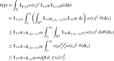 \begin{align}h({\boldsymbol{y}})&=\int_\mathbb{X} \unicode{x1d7d9}_{{\boldsymbol{y}}\preceq {\boldsymbol{x}}} w(t_x)^\zeta\unicode{x1d7d9}_{x\in W}\unicode{x1d7d9}_{t_x\le a} \mu({\textrm{d}} {\boldsymbol{x}})\\&=\unicode{x1d7d9}_{t_y \le a} \int_{t_y}^a \left(\int_{\mathbb{R}^d} \unicode{x1d7d9}_{x \in B_{v_y(t_x-t_y)}(y)}\unicode{x1d7d9}_{x\in W} \;{\textrm{d}} x \right) w(t_x)^\zeta\; \theta({\textrm{d}} t_x)\\& \le \unicode{x1d7d9}_{y \in W+B_{v_y(a-t_y)}(0)} \int_{t_y}^\infty\int_{\mathbb{R}^d}\unicode{x1d7d9}_{x \in B_{v_y(t_x-t_y)}(y)} w(t_x)^\zeta\;{\textrm{d}} x \theta({\textrm{d}} t_x) \\& \le \unicode{x1d7d9}_{y \in W+B_{v_y(a-t_y)}(0)} \int_{t_y}^\infty\omega_d v_y^d t_x^d w(t_x)^\zeta \;\theta({\textrm{d}} t_x) \\&\le \unicode{x1d7d9}_{y \in W+B_{v_y a}(0)} \omega_d Q(d,\zeta\nu_{d}) \, v_y^d.\end{align}
Therefore, the function G defined at (4.3) for
![]() $a \in (0,\infty)$
is bounded by
$a \in (0,\infty)$
is bounded by
 \begin{align}G({\boldsymbol{y}}) &\le \unicode{x1d7d9}_{y \in W} + \unicode{x1d7d9}_{y \in W+B_{v_y a}(0)} (1+\omega_d Q(d,\zeta\nu_{d}) \, v_y^d)(1+\omega_d^4 Q(d,\zeta\nu_{d})^4 \, v_y^{4d})\nonumber\\& \le 6 \omega_d^5 \unicode{x1d7d9}_{y \in W+B_{v_y a}(0)}p(v_y)\,,\end{align}
with
Define
In particular,
and
Recall V(W) defined at (2.4), and let
![]() $\omega=\max_{0 \le j \le d} \omega_j$
. The Steiner formula (see [Reference Schneider19, Section 4.1]) yields that
$\omega=\max_{0 \le j \le d} \omega_j$
. The Steiner formula (see [Reference Schneider19, Section 4.1]) yields that
 \begin{align}\int_{\mathbb{R}_+}\lambda(W+B_{v_xa}(0)) p(v_x) \nu({\textrm{d}} v_x)&= \sum_{i=0}^d \int_{\mathbb{R}_+}\omega_i v_x^i a^i V_{d-i}(W) \,p(v_x)\nu({\textrm{d}} v_x) \nonumber\\&\le \omega (1+a^d) \sum_{i=0}^d V_{d-i}(W) M_i \end{align}
with
![]() $c_d=(d+1)\omega$
, where in the final step we have used the simple inequality
$c_d=(d+1)\omega$
, where in the final step we have used the simple inequality
![]() $v_x^a \le 1+v_x^b$
for any
$v_x^a \le 1+v_x^b$
for any
![]() $0\le a\le b<\infty$
. We will use this fact many times in the sequel without mentioning it explicitly.
$0\le a\le b<\infty$
. We will use this fact many times in the sequel without mentioning it explicitly.
We will also often use the fact that for an increasing function f of the speed v, since p is also increasing, by positive association, we have
Lemma 4.2. For
![]() $a \in (0,\infty)$
,
$a \in (0,\infty)$
,
![]() $\alpha>0$
, and
$\alpha>0$
, and
![]() $f_\alpha^{(1)}$
defined at (4.5),
$f_\alpha^{(1)}$
defined at (4.5),
where
 \begin{align}C_1&\,:\!=\,C (1+a^d) M \frac{Q(0,\alpha \nu_{d}/2)}{\alpha},\\C_2&\,:\!=\,C (1+a^d) \, M_0 M \nu_{2d} Q(d,\alpha\nu_{d}/2)^2 Q(0,\alpha\nu_{d}),\end{align}
for a constant
![]() $C \in (0,\infty)$
depending only on d.
$C \in (0,\infty)$
depending only on d.
Proof. Using (4.9), we can write
 \begin{equation*}\int_{\mathbb{X}} f_\alpha^{(1)}({\boldsymbol{y}})\mu({\textrm{d}} {\boldsymbol{y}}) = \int_{\mathbb{X}}\int_{{\boldsymbol{y}}\preceq {\boldsymbol{x}}} G({\boldsymbol{x}})w(t_{x})^\alpha \mu({\textrm{d}} {\boldsymbol{x}})\mu({\textrm{d}} {\boldsymbol{y}})\\\le 6 \omega_d^5 \nu_{d} \int_{\mathbb{X}} \Lambda(t_x) \unicode{x1d7d9}_{x \in W+B_{v_xa}(0)}p(v_x) w(t_{x})^\alpha \mu({\textrm{d}} {\boldsymbol{x}}) \,=\!:\, 6 \omega_d^5 \nu_{d} \, I_1,\end{equation*}
whence, using (4.11) and the fact that
![]() $xe^{-x/2} \le 1$
for
$xe^{-x/2} \le 1$
for
![]() $x \in \mathbb{R}_+$
, we obtain
$x \in \mathbb{R}_+$
, we obtain
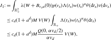 \begin{align}I_1 :&=\int_{\mathbb{R}_+^2}\lambda(W+B_{v_xa}(0)) p(v_x) \Lambda(t_x)w(t_{x})^\alpha \theta({\textrm{d}} t_x) \nu({\textrm{d}} v_x)\\&\le c_d (1+a^d) M \, V(W) \int_{\mathbb{R}_+} \Lambda(t_x)w(t_{x})^\alpha \theta({\textrm{d}} t_x) \\&\le c_d (1+a^d) M \frac{Q(0,\alpha \nu_{d}/2)}{\alpha \nu_{d}}\, V(W),\end{align}
proving the first assertion.
For the second assertion, first, by (3.2), for any
![]() $t_1,t_2 \in \mathbb{R}_+$
we have
$t_1,t_2 \in \mathbb{R}_+$
we have
 \begin{align}\int_{\mathbb{R}^d}&\mu(L_{0,t_1}\cap L_{x,t_2}){\textrm{d}} x=\int_0^{t_1\wedge t_2} \theta({\textrm{d}} s)\int_0^\infty \nu({\textrm{d}} v)\int_{\mathbb{R}^d} \lambda(B_{v(t_1-s)}(0)\cap B_{v(t_2-s)}(x)){\textrm{d}} x \nonumber\\&=\omega_d^2 \int_0^\infty v^{2d}\nu({\textrm{d}} v) \int_0^{t_1\wedge t_2}(t_1-s)^d(t_2-s)^d\theta({\textrm{d}} s) \nonumber\\&=\omega_d^2\nu_{2d} \int_0^{t_1\wedge t_2}(t_1-s)^d(t_2-s)^d\theta({\textrm{d}} s)\,=\!:\, \ell(t_1,t_2),\end{align}
which is symmetric in
![]() $t_1$
and
$t_1$
and
![]() $t_2$
. Thus, changing the order of the integrals in the second step and using (4.9) for the final step, we get
$t_2$
. Thus, changing the order of the integrals in the second step and using (4.9) for the final step, we get
 \begin{align}\int_{\mathbb{X}} &f_\alpha^{(1)}({\boldsymbol{y}})^2\mu({\textrm{d}} {\boldsymbol{y}})=\int_{\mathbb{X}}\int_{{\boldsymbol{y}}\preceq {\boldsymbol{x}}_1}\int_{{\boldsymbol{y}}\preceq {\boldsymbol{x}}_2} G({\boldsymbol{x}}_1)w(t_{x_1})^\alpha G({\boldsymbol{x}}_2)w(t_{x_2})^\alpha \mu({\textrm{d}} {\boldsymbol{x}}_1)\mu({\textrm{d}} {\boldsymbol{x}}_2)\mu({\textrm{d}} {\boldsymbol{y}})\nonumber\\&=\int_\mathbb{X}\int_\mathbb{X}\left(\int_{{\boldsymbol{y}}\preceq {\boldsymbol{x}}_1,{\boldsymbol{y}}\preceq{\boldsymbol{x}}_2}\mu({\textrm{d}} {\boldsymbol{y}})\right)G({\boldsymbol{x}}_1)G({\boldsymbol{x}}_2)\big(w(t_{x_1})w(t_{x_2}) \big)^\alpha\mu({\textrm{d}} {\boldsymbol{x}}_1)\mu({\textrm{d}} {\boldsymbol{x}}_2)\nonumber\\&=\int_\mathbb{X}\int_\mathbb{X}\mu(L_{x_1,t_{x_1}}\cap L_{x_2,t_{x_2}})G({\boldsymbol{x}}_1)G({\boldsymbol{x}}_2)\big (w(t_{x_1})w(t_{x_2}) \big)^\alpha\mu({\textrm{d}} {\boldsymbol{x}}_1)\mu({\textrm{d}} {\boldsymbol{x}}_2)\nonumber\\&\leq 36 \omega_d^{10} \, M_0 I_2,\end{align}
where
 \begin{equation*}I_2\,:\!=\,\int_{\mathbb{R}_+^3}\left(\int_{\mathbb{R}^d} \left(\int_{\mathbb{R}^d}\mu(L_{0,t_{x_1}}\cap L_{x_2-x_1,t_{x_2}}) {\textrm{d}} x_2 \right)\unicode{x1d7d9}_{x_1 \in W + B_{v_{x_1}a}(0)} {\textrm{d}} x_1 \right)\\\times p(v_{x_1}) \big (w(t_{x_1})w(t_{x_2}) \big)^\alpha\theta^2({\textrm{d}} (t_{x_1}, t_{x_2}) \nu ({\textrm{d}} v_{x_1}).\end{equation*}
 \begin{align}I_2&=\int_{\mathbb{R}_+^3} \ell(t_{x_1},t_{x_2})\lambda(W + B_{v_{x_1}a}(0)) p(v_{x_1}) \big (w(t_{x_1})w(t_{x_2}) \big)^\alpha\theta^2({\textrm{d}} (t_{x_1}, t_{x_2}) \nu ({\textrm{d}} v_{x_1})\\& \le c_d (1+a^d) M \, V(W) \,\int_{\mathbb{R}_+^2} \ell(t_{x_1},t_{x_2}) \big (w(t_{x_1})w(t_{x_2}) \big)^\alpha \theta^2({\textrm{d}} (t_{x_1}, t_{x_2})).\end{align}
Using that w is a decreasing function, the result now follows from (4.13) and (4.12) by noticing that
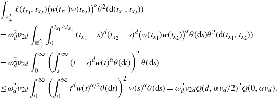 \begin{align}&\int_{\mathbb{R}_+^2} \ell(t_{x_1},t_{x_2}) \big (w(t_{x_1})w(t_{x_2}) \big)^\alpha \theta^2({\textrm{d}} (t_{x_1}, t_{x_2})) \\&= \omega_d^{2} \nu_{2d}\int_{\mathbb{R}_+^2}\int_0^{t_{x_1}\wedge t_{x_2}}(t_{x_1}-s)^d(t_{x_2}-s)^d\big (w(t_{x_1})w(t_{x_2}) \big)^\alpha\theta({\textrm{d}} s) \theta^2({\textrm{d}} (t_{x_1}, t_{x_2}))\\&=\omega_d^{2} \nu_{2d}\int_0^\infty \left(\int_s^\infty(t-s)^dw(t)^\alpha\theta({\textrm{d}} t)\right)^2\theta({\textrm{d}} s) \\& \le \omega_d^{2} \nu_{2d}\int_0^\infty \left(\int_0^\infty t^dw(t)^{\alpha/2}\theta({\textrm{d}} t)\right)^2 w(s)^\alpha\theta({\textrm{d}} s) = \omega_d^{2}\nu_{2d} Q(d,\alpha\nu_{d}/2)^2 Q(0,\alpha\nu_{d}).\end{align}
Arguing as in (4.11), we also have
 \begin{align}\int_{\mathbb{R}_+}\lambda(W+B_{v_xa}(0)) v_x^d p(v_x) \nu({\textrm{d}} v_x) &\le \omega (1+a^d) \sum_{i=0}^d V_{d-i}(W) M_{d+i}\end{align}
with
Note that by positive association, we have
![]() $\nu_{d} M \le M'$
.
$\nu_{d} M \le M'$
.
Lemma 4.3. For
![]() $a \in (0,\infty)$
,
$a \in (0,\infty)$
,
![]() $\alpha>0$
, and
$\alpha>0$
, and
![]() $f_\alpha^{(2)}$
defined at (4.5),
$f_\alpha^{(2)}$
defined at (4.5),
for
for a constant
![]() $C \in (0,\infty)$
depending only on d.
$C \in (0,\infty)$
depending only on d.
Proof. By the definition of
![]() $f_\alpha^{(2)}$
, (4.9), and (4.15), we obtain
$f_\alpha^{(2)}$
, (4.9), and (4.15), we obtain
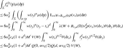 \begin{align}&\int_{\mathbb{X}} f_\alpha^{(2)}({\boldsymbol{y}}) \mu({\textrm{d}} {\boldsymbol{y}})\\&\leq 6 \omega_d^5 \,\int_\mathbb{X}\left(\int_{{\boldsymbol{x}}\preceq {\boldsymbol{y}}} w(t_y)^{\alpha} \mu({\textrm{d}}{\boldsymbol{y}})\right)\unicode{x1d7d9}_{x \in W+B_{v_xa}(0)} p(v_x) \mu({\textrm{d}} {\boldsymbol{x}})\\&=6 \omega_d^6\int_0^\infty \int_{t_x}^\infty w(t_y)^\alpha (t_y-t_x)^d \int_0^\infty \lambda(W+B_{v_xa}(0)) v_x^d p(v_x) \nu({\textrm{d}} v_x) \theta({\textrm{d}} t_y)\theta({\textrm{d}} t_x) \\& \le 6 \omega_d^6 c_d (1+a^d) M' \, V(W)\int_0^\infty w(t_x)^{\alpha/2} \theta({\textrm{d}} t_x)\int_{0}^\infty t_y^d w(t_y)^{\alpha/2} \theta({\textrm{d}} t_y)\\&\le 6 \omega_d^6 c_d (1+a^d) M' \,Q(0,\alpha\nu_{d}/2)Q(d,\alpha\nu_{d}/2)\, V(W),\end{align}
where in the penultimate step we have used that w is decreasing. This proves the first assertion.
For the second assertion, using (4.9), we have
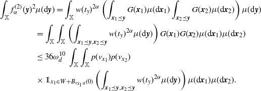 \begin{align}\int_\mathbb{X} f_\alpha^{(2)}({\boldsymbol{y}})^2&\mu({\textrm{d}} {\boldsymbol{y}})=\int_\mathbb{X} w(t_y)^{2\alpha} \left(\int_{{\boldsymbol{x}}_1\preceq {\boldsymbol{y}}}G({\boldsymbol{x}}_1)\mu({\textrm{d}} {\boldsymbol{x}}_1)\int_{{\boldsymbol{x}}_2\preceq {\boldsymbol{y}}}G({\boldsymbol{x}}_2)\mu({\textrm{d}} {\boldsymbol{x}}_2)\right)\mu({\textrm{d}} {\boldsymbol{y}})\nonumber\\&=\int_\mathbb{X}\int_\mathbb{X}\left(\int_{{\boldsymbol{x}}_1\preceq {\boldsymbol{y}},{\boldsymbol{x}}_2\preceq{\boldsymbol{y}}}w(t_y)^{2\alpha}\mu({\textrm{d}}{\boldsymbol{y}})\right)G({\boldsymbol{x}}_1)G({\boldsymbol{x}}_2)\mu({\textrm{d}} {\boldsymbol{x}}_1)\mu({\textrm{d}} {\boldsymbol{x}}_2)\nonumber\\&\leq 36 \omega_d^{10} \,\int_\mathbb{X}\int_\mathbb{X}p(v_{x_1})p(v_{x_2})\nonumber\\&\times\unicode{x1d7d9}_{x_1 \in W+B_{v_{x_1}a}(0)}\left(\int_{{\boldsymbol{x}}_1\preceq {\boldsymbol{y}},{\boldsymbol{x}}_2\preceq{\boldsymbol{y}}}w(t_y)^{2\alpha}\mu({\textrm{d}} {\boldsymbol{y}})\right)\mu({\textrm{d}} {\boldsymbol{x}}_1)\mu({\textrm{d}} {\boldsymbol{x}}_2).\end{align}
For fixed
![]() ${\boldsymbol{x}}_1$
,
${\boldsymbol{x}}_1$
,
![]() $t_{x_2}$
, and
$t_{x_2}$
, and
![]() $v_{x_2}$
, we have
$v_{x_2}$
, we have
 \begin{align}&\int_{\mathbb{R}^d}\int_{{\boldsymbol{x}}_1\preceq {\boldsymbol{y}},{\boldsymbol{x}}_2\preceq{\boldsymbol{y}}}w(t_y)^{2\alpha} \mu({\textrm{d}}{\boldsymbol{y}}){\textrm{d}} x_2\\&=\int_{t_{x_1}\vee t_{x_2}}^\infty w(t_y)^{2\alpha}\left(\int_{\mathbb{R}^d}\lambda \big (B_{v_{x_1}(t_y-t_{x_1})}(0)\cap B_{v_{x_2}(t_y-t_{x_2})}(x) \big){\textrm{d}} x\right)\theta({\textrm{d}} t_y)\\&=\omega_d^2 v_{x_1}^d v_{x_2}^d \int_{t_{x_1}\vee t_{x_2}}^\infty(t_y-t_{x_1})^d(t_y-t_{x_2})^d w(t_y)^{2\alpha} \theta({\textrm{d}} t_y)\,.\end{align}
Arguing similarly as for
![]() $\mu(f_\alpha^{(2)})$
above, we obtain from (4.16) and (4.15) that
$\mu(f_\alpha^{(2)})$
above, we obtain from (4.16) and (4.15) that
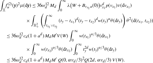 \begin{align}\int_\mathbb{X} &f_\alpha^{(2)}({\boldsymbol{y}})^2 \mu({\textrm{d}} {\boldsymbol{y}})\leq 36 \omega_d^{12} \,M_d\int_0^\infty \lambda \big (W+B_{v_{x_1}a}(0) \big) v_{x_1}^d p(v_{x_1})\nu({\textrm{d}} v_{x_1})\\&\qquad\qquad\times\int_{\mathbb{R}_+^2} \left(\int_{t_{x_1}\vee t_{x_2}}^\infty (t_y-t_{x_1})^d(t_y-t_{x_2})^dw(t_y)^\alpha \theta({\textrm{d}} t_y)\right)\theta^2({\textrm{d}} (t_{x_1},t_{x_2}))\\&\leq 36 \omega_d^{12} c_d (1+a^d) \,M_d M' V(W)\int_0^\infty w(t_{x_1})^{\alpha/3} \theta({\textrm{d}} t_{x_1})\\& \qquad \qquad \times \int_0^\infty w(t_{x_2})^{\alpha/3} \theta({\textrm{d}} t_{x_2}) \int_0^\infty t_y^{2d}w(t_y)^{\alpha/3}\theta({\textrm{d}} t_y)\\&\le 36 \omega_d^{12} c_d (1+a^d) \,M_d M'\,Q(0,\alpha\nu_{d}/3)^2 Q(2d,\alpha\nu_{d}/3)\, V(W).\end{align}
Before proceeding to bound the integrals of
![]() $f^{(3)}$
, notice that, since
$f^{(3)}$
, notice that, since
![]() $\theta$
is a non-null measure,
$\theta$
is a non-null measure,
 \begin{multline}M^{\prime}_{\alpha}=M^{\prime}_{\alpha}(\nu_{d})\,:\!=\,\int_0^\infty t^{d-1} e^{-\frac{\alpha\nu_{d}}{3}\Lambda(t)} {\textrm{d}} t=\int_0^\infty t^{d-1} e^{-\frac{\alpha\omega_d \nu_{d}}{3}\int_0^t (t-s)^d\theta({\textrm{d}} s)} {\textrm{d}} t\\\leq \int_0^\infty t^{d-1} e^{-\frac{\alpha\omega_d \nu_{d}}{3}\int_0^{t/2} (t/2)^d\theta({\textrm{d}} s)} {\textrm{d}} t=\int_0^\infty t^{d-1} e^{-\frac{\alpha\omega_d \nu_{d}}{3}\,\theta([0,t/2))(t/2)^d} {\textrm{d}} t<\infty\,.\end{multline}
Lemma 4.4. For
![]() $a \in (0,\infty)$
,
$a \in (0,\infty)$
,
![]() $\alpha \in (0,1]$
, and
$\alpha \in (0,1]$
, and
![]() $f_\alpha^{(3)}$
defined at (4.5),
$f_\alpha^{(3)}$
defined at (4.5),
where
 \begin{align}C_1&\,:\!=\,C\, (1+a^d) M' Q(0,\alpha\nu_{d}/3)^2\Big[M^{\prime}_{\alpha} +Q(2d,\alpha\nu_{d}/3)\nu_{d} \Big]\,,\\C_2&\,:\!=\,C\, (1+a^d) M_d M' (1+\nu_{2d}\nu_{d}^{-2})Q(0,\alpha\nu_{d}/3)^3 \\&\qquad \qquad\qquad\times \left({M^{\prime}_{\alpha}}^2+M^{\prime}_{\alpha} Q(2d,\alpha\nu_{d}/3) \nu_{d} +Q(2d,\alpha\nu_{d}/3)^2 \nu_{2d}\right),\end{align}
for a constant
![]() $C \in (0,\infty)$
depending only on d.
$C \in (0,\infty)$
depending only on d.
Proof. Note that
![]() ${\boldsymbol{x}},{\boldsymbol{y}} \preceq {\boldsymbol{z}}$
implies
${\boldsymbol{x}},{\boldsymbol{y}} \preceq {\boldsymbol{z}}$
implies
For q defined at (4.4), we have
where
Therefore,
 \begin{align}q({\boldsymbol{x}},{\boldsymbol{y}})^\alpha&\leq e^{-\alpha\nu_{d} \Lambda(r_0)} \nonumber \\& \qquad \times \left(1+\int_{r_0}^\infty \lambda \big (B_{v_x(t_z-t_x)}(0) \cap B_{v_y(t_z-t_y)}(y-x) \big)e^{-\nu_{d} (\Lambda(t_z)-\Lambda(r_0))} \theta({\textrm{d}} t_z)\right)\nonumber\\&\leq e^{-\alpha\nu_{d} \Lambda(r_0)}+ \int_{r_0}^\infty \lambda \big (B_{v_x(t_z-t_x)}(0) \cap B_{v_y(t_z-t_y)}(y-x) \big)e^{-\alpha\nu_{d} \Lambda(t_z)} \theta({\textrm{d}} t_z)\,.\end{align}
Then, with
![]() $f_\alpha^{(3)}$
defined at (4.5),
$f_\alpha^{(3)}$
defined at (4.5),
 \begin{align}\int_\mathbb{X} &f_\alpha^{(3)}({\boldsymbol{y}})\mu({\boldsymbol{y}})\leq\int_{\mathbb{X}^2} G({\boldsymbol{x}})e^{-\alpha\nu_{d} \Lambda(r_0)}\mu^2({\textrm{d}}({\boldsymbol{x}}, {\boldsymbol{y}}))\nonumber\\&\quad +\int_{\mathbb{X}^2} G({\boldsymbol{x}})\int_{r_0}^\infty\lambda \big (B_{v_x(t_z-t_x)}(0) \cap B_{v_y(t_z-t_y)}(y-x) \big)e^{-\alpha\nu_{d} \Lambda(t_z)} \theta({\textrm{d}} t_z)\mu^2({\textrm{d}}({\boldsymbol{x}}, {\boldsymbol{y}})).\end{align}
Since
![]() $\Lambda$
is increasing,
$\Lambda$
is increasing,
and, by a change of variable and passing to polar coordinates, we obtain
Thus, using (4.9), (4.20), and (4.21), we can bound the first summand on the right-hand side of (4.19) as
 \begin{align}\int_{\mathbb{X}^2} G({\boldsymbol{x}})&e^{-\alpha\nu_{d} \Lambda(r_0)}\mu^2({\textrm{d}}({\boldsymbol{x}}, {\boldsymbol{y}}))\leq6 \omega_d^5\int_0^\infty e^{-\frac{\alpha\nu_{d} }{3}\Lambda(t_x)}{\textrm{d}} t_x\int_0^\infty e^{-\frac{\alpha\nu_{d} }{3}\Lambda(t_y)} {\textrm{d}} t_y\\&\quad \times \int_{\mathbb{R}^d}\unicode{x1d7d9}_{x \in W+B_{v_x a}(0)} {\textrm{d}} x\iint_{\mathbb{R}_+^2\times\mathbb{R}^d} p(v_x)e^{-\frac{\alpha\nu_{d} }{3}\Lambda\left(\frac{|x-y|}{v_x+v_y}\right)}{\textrm{d}} y\,\nu^2({\textrm{d}} (v_x, v_y))\\&\leq6 \omega_d^6 d Q(0,\alpha\nu_{d}/3)^2 M^{\prime}_{\alpha}\,\int_{\mathbb{R}_+^2}\lambda \big (W+B_{v_x a}(0) \big) p(v_x)(v_x+v_y)^d\nu^2({\textrm{d}} (v_x, v_y))\\&\leq 2^{d+3} \omega_d^6 d c_d (1+a^d) M' M^{\prime}_{\alpha} Q(0,\alpha\nu_{d}/3)^2\,V(W)\,,\end{align}
where for the final step we have used Jensen’s inequality, (4.11) and (4.15), and the fact that
![]() $\nu_{d} M \le M'$
. Arguing similarly for the second summand in (4.19), using (4.9) and the fact that
$\nu_{d} M \le M'$
. Arguing similarly for the second summand in (4.19), using (4.9) and the fact that
![]() $r_0 \ge t_x \vee t_y$
in the first step, (3.2) in the second step, and (4.15) in the final step, we obtain
$r_0 \ge t_x \vee t_y$
in the first step, (3.2) in the second step, and (4.15) in the final step, we obtain
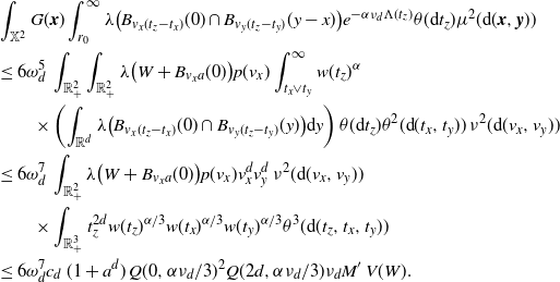 \begin{align}&\int_{\mathbb{X}^2} G({\boldsymbol{x}})\int_{r_0}^\infty\lambda \big (B_{v_x(t_z-t_x)}(0) \cap B_{v_y(t_z-t_y)}(y-x) \big)e^{-\alpha\nu_{d} \Lambda(t_z)} \theta({\textrm{d}} t_z)\mu^2({\textrm{d}}({\boldsymbol{x}}, {\boldsymbol{y}}))\\&\leq 6 \omega_d^5\,\int_{\mathbb{R}_+^2} \int_{\mathbb{R}_+^2} \lambda \big ( W+B_{v_x a}(0) \big) p(v_x) \int_{t_x\vee t_y}^\infty w(t_z)^\alpha\\&\qquad \times \left(\int_{\mathbb{R}^d}\lambda \big (B_{v_x(t_z-t_x)}(0) \cap B_{v_y(t_z-t_y)}(y) \big){\textrm{d}} y\right) \theta({\textrm{d}} t_z) \theta^2( {\textrm{d}} (t_x, t_y))\,\nu^2({\textrm{d}} (v_x, v_y))\\&\leq 6 \omega_d^7 \,\int_{\mathbb{R}_+^2} \lambda \big ( W+B_{v_x a}(0) \big) p(v_x) v_x^d v_y^d\,\nu^2({\textrm{d}} (v_x, v_y))\\&\qquad\times\int_{\mathbb{R}_+^3} t_z^{2d}w(t_z)^{\alpha/3}w(t_x)^{\alpha/3}w(t_y)^{\alpha/3}\theta^3({\textrm{d}} (t_z, t_x, t_y))\\&\leq6 \omega_d^7 c_d \, (1+a^d) \, Q(0,\alpha\nu_{d}/3)^2Q(2d,\alpha\nu_{d}/3)\nu_{d} M'\,V(W).\end{align}
This concludes the proof of the first assertion.
Next, we prove the second assertion. For ease of notation, we drop obvious subscripts and write
![]() ${\boldsymbol{y}}=(y,s,v)$
,
${\boldsymbol{y}}=(y,s,v)$
,
![]() ${\boldsymbol{x}}_1=(x_1,t_1,u_1)$
, and
${\boldsymbol{x}}_1=(x_1,t_1,u_1)$
, and
![]() ${\boldsymbol{x}}_2=(x_2,t_2,u_2)$
. Using (4.18), write
${\boldsymbol{x}}_2=(x_2,t_2,u_2)$
. Using (4.18), write
 \begin{align}\int_\mathbb{X} f_\alpha^{(3)}({\boldsymbol{y}})^2\mu({\boldsymbol{y}})&=\int_{\mathbb{X}^3} G({\boldsymbol{x}}_1)G({\boldsymbol{x}}_2)q({\boldsymbol{x}}_1,{\boldsymbol{y}})^\alpha q({\boldsymbol{x}}_2,{\boldsymbol{y}})^\alpha\mu^3({\textrm{d}} ({\boldsymbol{x}}_1, {\boldsymbol{x}}_2, {\boldsymbol{y}}))\nonumber\\&\leq \int_{\mathbb{X}^3} G({\boldsymbol{x}}_1)G({\boldsymbol{x}}_2)(\mathfrak I_1+2\mathfrak I_2+\mathfrak I_3)\mu^3({\textrm{d}} ({\boldsymbol{x}}_1, {\boldsymbol{x}}_2, {\boldsymbol{y}}))\,,\end{align}
with
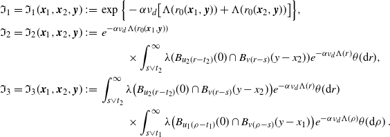 \begin{align}\mathfrak I_1&=\mathfrak I_1({\boldsymbol{x}}_1,{\boldsymbol{x}}_2,{\boldsymbol{y}})\,:\!=\,\exp\Big\{-\alpha\nu_{d} \big[\Lambda(r_0({\boldsymbol{x}}_1,{\boldsymbol{y}}))+\Lambda(r_0({\boldsymbol{x}}_2,{\boldsymbol{y}}))\big]\Big\},\\\mathfrak I_2&=\mathfrak I_2({\boldsymbol{x}}_1,{\boldsymbol{x}}_2,{\boldsymbol{y}})\,:\!=\,e^{-\alpha\nu_{d} \Lambda(r_0({\boldsymbol{x}}_1,{\boldsymbol{y}}))}\\&\qquad\qquad\qquad\qquad\qquad\times\int_{s\vee t_2}^\infty\lambda(B_{u_2(r-t_2)}(0)\cap B_{v(r-s)}(y-x_2))e^{-\alpha\nu_{d} \Lambda(r)} \theta( {\textrm{d}} r),\\\mathfrak I_3&=\mathfrak I_3({\boldsymbol{x}}_1,{\boldsymbol{x}}_2,{\boldsymbol{y}})\,:\!=\,\int_{s\vee t_2}^\infty\lambda \big (B_{u_2(r-t_2)}(0)\cap B_{v(r-s)}(y-x_2) \big)e^{-\alpha\nu_{d} \Lambda(r)} \theta({\textrm{d}} r)\;\\&\qquad\qquad\qquad\qquad\qquad\times\int_{s\vee t_1}^\infty\lambda \big (B_{u_1(\rho-t_1)}(0)\cap B_{v(\rho-s)}(y-x_1) \big)e^{-\alpha\nu_{d} \Lambda(\rho)} \theta({\textrm{d}} \rho)\,.\end{align}
By (4.21),
 \begin{align}&\iint_{\mathbb{R}^{2d}}\exp\Big\{-\frac{\alpha\nu_{d} }{3}\left[\Lambda\left(\frac{|y|}{u_1+v}\right)+\Lambda\left(\frac{|x-y|}{u_2+v}\right)\right]\Big\}\,{\textrm{d}} x {\textrm{d}} y\\&\leq\int_{\mathbb{R}^d} \exp\Big\{-\frac{\alpha\nu_{d} }{3}\Lambda\left(\frac{|y|}{u_1+v}\right)\Big\}{\textrm{d}} y\int_{\mathbb{R}^d} \exp\Big\{-\frac{\alpha\nu_{d} }{3}\Lambda\left(\frac{|x|}{u_2+v}\right)\Big\}{\textrm{d}} x\\&\leq {d}^2{\omega}_d^2 {(u_1+v)}^d {(u_2+v)}^d{M^{\prime}_{\alpha}}^2.\end{align}
Hence, using (4.9) and (4.20) for the first step, we have
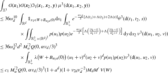 \begin{align}&\int_{\mathbb{X}^3} G({\boldsymbol{x}}_1)G({\boldsymbol{x}}_2) \mathfrak I_1({\boldsymbol{x}}_1,{\boldsymbol{x}}_2,{\boldsymbol{y}})\ \mu^3({\textrm{d}} ({\boldsymbol{x}}_1,{\boldsymbol{x}}_2,{\boldsymbol{y}}))\\&\leq 36 \omega_d^{10}\, \int_{\mathbb{R}^{d}} \unicode{x1d7d9}_{x_1 \in W+B_{u_1 a}(0)} {\textrm{d}} x_1\int_{\mathbb{R}_+^3} e^{-\frac{\alpha\nu_{d} }{3} \left[\Lambda(t_1)+\Lambda(t_2)+2\Lambda(s)\right]}\theta^3({\textrm{d}} (t_1, t_2,s))\\&\qquad\qquad\times \iint_{{\mathbb{R}}_+^3\times{(\mathbb{R}^d)}^2}p(u_1) p(u_2)e^{-\frac{\alpha\nu_{d}}{3}\left[ \Lambda\left(\frac{|x_1-y|}{u_1+v}\right) +\Lambda\left(\frac{|x_2-y|}{u_2+v}\right)\right]}\,{\textrm{d}} y\,{\textrm{d}} x_2\,\nu^3({\textrm{d}} (u_1,u_2,v))\\&\leq 36 {\omega}_d^{12} {d}^2\,M_{{\alpha}}^{'2}Q{(0,\alpha\nu_{d}/3)}^{3} \\& \qquad\qquad \times \int_{\mathbb{R}_+^3} \lambda \big (W+B_{u_1 a}(0) \big)\,{(u_1+v)}^d {(u_2+v)}^dp(u_1) p(u_2)\nu^3({\textrm{d}} (u_1,u_2,v))\\&\leq c_1 \,M_{{\alpha}}^{'2}Q{(0,\alpha\nu_{d}/3)}^{3} (1+{a}^d) (1+\nu_{2d}\nu_{d}^{-2}) M_d M' \, V(W)\,\end{align}
for some constant
![]() $c_1 \in (0,\infty)$
depending only on d. Here we have used the monotonicity of Q with respect to its second argument in the penultimate step, and in the final step we have used Jensen’s inequality and (4.15) along with the fact that
$c_1 \in (0,\infty)$
depending only on d. Here we have used the monotonicity of Q with respect to its second argument in the penultimate step, and in the final step we have used Jensen’s inequality and (4.15) along with the fact that
for some constant
![]() $C \in (0,\infty)$
depending only on d.
$C \in (0,\infty)$
depending only on d.
Next we bound the second summand in (4.22). Using (3.2) in the second step, the monotonicity of
![]() $\Lambda$
and (4.20) in the third step, and (4.21) in the final step, we have
$\Lambda$
and (4.20) in the third step, and (4.21) in the final step, we have
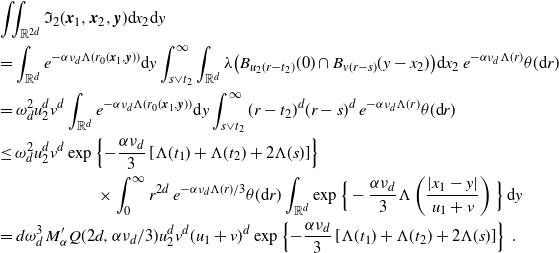 \begin{align}&\iint_{\mathbb{R}^{2d}} \mathfrak I_2({\boldsymbol{x}}_1,{\boldsymbol{x}}_2,{\boldsymbol{y}}) {\textrm{d}} x_2 {\textrm{d}} y\\&=\int_{\mathbb{R}^{d}}e^{-\alpha\nu_{d} \Lambda(r_0({\boldsymbol{x}}_1,{\boldsymbol{y}}))} {\textrm{d}} y\int_{s\vee t_2}^\infty\int_{\mathbb{R}^d}\lambda \big (B_{u_2(r-t_2)}(0) \cap B_{v(r-s)}(y-x_2) \big) {\textrm{d}} x_2\,e^{-\alpha\nu_{d} \Lambda(r)} \theta({\textrm{d}} r)\\&=\omega_d^2 u_2^d v^d \int_{\mathbb{R}^{d}}e^{-\alpha\nu_{d} \Lambda(r_0({\boldsymbol{x}}_1,{\boldsymbol{y}}))} {\textrm{d}} y\int_{s\vee t_2}^\infty (r-t_2)^d (r-s)^d\,e^{-\alpha\nu_{d} \Lambda(r)} \theta({\textrm{d}} r)\\&\le \omega_d^2 u_2^d v^d \exp\left\{-\frac{\alpha\nu_{d} }{3}\left[\Lambda(t_1)+\Lambda(t_2)+2\Lambda(s)\right]\right\}\\&\qquad \qquad \qquad \times \int_0^\infty r^{2d}\,e^{-\alpha\nu_{d} \Lambda(r)/3} \theta({\textrm{d}} r)\int_{\mathbb{R}^d} \exp\Big\{-\frac{\alpha\nu_{d} }{3}\Lambda\left(\frac{|x_1-y|}{u_1+v}\right)\Big\}\,{\textrm{d}} y\\&=d \omega_d^3 \,M^{\prime}_{\alpha} Q(2d,\alpha\nu_{d}/3)u_2^d v^d (u_1+v)^d\exp\left\{-\frac{\alpha \nu_{d} }{3}\left[\Lambda(t_1)+\Lambda(t_2)+2\Lambda(s)\right]\right\}\,.\end{align}
Therefore, arguing similarly as before, we obtain
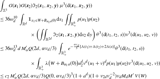 \begin{align}&\int_{\mathbb{X}^3} G({\boldsymbol{x}}_1)G({\boldsymbol{x}}_2) \mathfrak I_2({\boldsymbol{x}}_1,{\boldsymbol{x}}_2,{\boldsymbol{y}})\ \mu^3({\textrm{d}} ({\boldsymbol{x}}_1, {\boldsymbol{x}}_2, {\boldsymbol{y}}))\\&\leq36 \omega_d^{10} \,\int_{\mathbb{R}^{d}}\unicode{x1d7d9}_{x_1 \in W+B_{u_1 a}(0)} {\textrm{d}} x_1\iint_{\mathbb{R}_+^6} p(u_1)p(u_2) \\& \qquad \qquad\qquad\times\left( \iint_{\mathbb{R}^{2d}} \mathfrak I_2({\boldsymbol{x}}_1,{\boldsymbol{x}}_2,{\boldsymbol{y}}){\textrm{d}} x_2\,{\textrm{d}} y \right)\theta^3 ({\textrm{d}} (t_1,t_2,s))\nu^3 ({\textrm{d}} (u_1,u_2,v))\\&\leq 36 \omega_d^{13} d \,M^{\prime}_{\alpha} Q(2d,\alpha\nu_{d}/3)\, \int_{\mathbb{R}_+^3}e^{-\frac{\alpha\nu_{d} }{3}\left[ \Lambda(t_1)+\Lambda(t_2)+2\Lambda(s)\right]}\theta^3 ({\textrm{d}}( t_1,t_2,s))\\&\qquad\qquad\qquad \times \int_{\mathbb{R}_+^3} \lambda \big (W+B_{u_1 a}(0) \big) u_2^dv^d (u_1+v)^d p(u_1)p(u_2)\nu^3 ({\textrm{d}} (u_1,u_2,v))\\&\leq c_2 \, M^{\prime}_{\alpha} Q(2d,\alpha\nu_{d}/3)Q(0,\alpha\nu_{d}/3)^{3} (1+a^d) (1+\nu_{2d}\nu_{d}^{-2}) \nu_{d} M_d M' \, V(W)\,\end{align}
for some constant
![]() $c_2 \in (0,\infty)$
depending only on d, where for the final step we have used
$c_2 \in (0,\infty)$
depending only on d, where for the final step we have used
for some constant
![]() $C' \in (0,\infty)$
depending only on d.
$C' \in (0,\infty)$
depending only on d.
Finally, we bound the third summand in (4.22). Arguing as above,
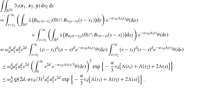 \begin{align}&\iint_{\mathbb{R}^{2d}} \mathfrak I_3({\boldsymbol{x}}_1,{\boldsymbol{x}}_2,{\boldsymbol{y}})\,{\textrm{d}} x_2\,{\textrm{d}} y\\&=\int_{s\vee t_1}^\infty\left(\int_{\mathbb{R}^d}\lambda \big (B_{u_1(\rho-t_1)}(0)\cap B_{v(\rho-s)}(y-x_1) \big) {\textrm{d}} y\right)e^{-\alpha\nu_{d} \Lambda(\rho)} \theta({\textrm{d}} \rho)\\&\qquad\qquad \qquad\times\int_{s\vee t_2}^\infty\left(\int_{\mathbb{R}^d}\lambda \big (B_{u_2(r-t_2)}(0) \cap B_{v(r-s)}(y-x_2) \big) {\textrm{d}} x_2\right)e^{-\alpha\nu_{d} \Lambda(r)} \theta({\textrm{d}} r)\\&=\omega_d^4 u_1^d u_2^d v^{2d}\int_{s\vee t_1}^\infty(\rho-t_1)^d(\rho-s)^de^{-\alpha\nu_{d} \Lambda(\rho)} \theta({\textrm{d}} \rho)\int_{s\vee t_2}^\infty(r-t_1)^d(r-s)^de^{-\alpha\nu_{d} \Lambda(r)} \theta({\textrm{d}} r)\\&\leq \omega_d^4 u_1^d u_2^d v^{2d} \left(\int_0^\infty r^{2d}\,e^{-\alpha\nu_{d} \Lambda(r)/3} \theta({\textrm{d}} r)\right)^2\exp\Big\{-\frac{\alpha}{3}\nu_{d} \big[\Lambda(t_1)+\Lambda(t_2)+2\Lambda(s)\big]\Big\}\\&\le \omega_d^4\,Q(2d,\alpha\nu_{d}/3)^2 u_1^d u_2^d v^{2d}\exp\Big\{-\frac{\alpha}{3} \nu_{d} \big[\Lambda(t_1)+\Lambda(t_2)+2\Lambda(s)\big]\Big\}\,.\end{align}
Thus,
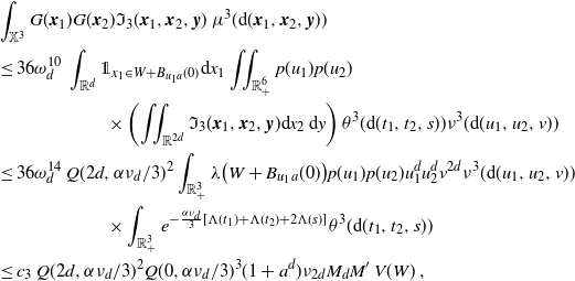 \begin{align}&\int_{\mathbb{X}^3} G({\boldsymbol{x}}_1)G({\boldsymbol{x}}_2) \mathfrak I_3({\boldsymbol{x}}_1,{\boldsymbol{x}}_2,{\boldsymbol{y}})\ \mu^3({\textrm{d}}( {\boldsymbol{x}}_1,{\boldsymbol{x}}_2,{\boldsymbol{y}}))\\&\leq 36 \omega_d^{10}\,\int_{\mathbb{R}^{d}} \unicode{x1d7d9}_{x_1 \in W+B_{u_1 a}(0)} {\textrm{d}} x_1\iint_{\mathbb{R}_+^6} p(u_1) p(u_2)\\&\qquad\qquad\qquad\times\left( \iint_{\mathbb{R}^{2d}} \mathfrak I_3({\boldsymbol{x}}_1,{\boldsymbol{x}}_2,{\boldsymbol{y}}) {\textrm{d}} x_2\,{\textrm{d}} y \right)\theta^3 ({\textrm{d}} (t_1,t_2,s))\nu^3 ({\textrm{d}} (u_1, u_2, v))\\&\leq 36 \omega_d^{14} \,Q(2d,\alpha\nu_{d}/3)^2\int_{\mathbb{R}_+^3} \lambda \big (W+B_{u_1 a}(0) \big)p(u_1) p(u_2)u_1^d u_2^d v^{2d}\nu^3 ({\textrm{d}} (u_1, u_2, v))\\&\qquad\qquad\qquad\times\int_{\mathbb{R}_+^3}e^{-\frac{\alpha\nu_{d} }{3}\left[ \Lambda(t_1)+\Lambda(t_2)+2\Lambda(s)\right]}\theta^3 ({\textrm{d}} (t_1,t_2,s))\\&\leq c_3\,Q(2d,\alpha\nu_{d}/3)^2 Q(0,\alpha\nu_{d}/3)^{3} (1+a^d)\nu_{2d} M_d M'\, V(W)\,,\end{align}
for some constant
![]() $c_3 \in (0,\infty)$
depending only on d. Combining the bounds for the summands on the right-hand side of (4.22) yields the desired conclusion.
$c_3 \in (0,\infty)$
depending only on d. Combining the bounds for the summands on the right-hand side of (4.22) yields the desired conclusion.
To compute the bounds in (4.6) and (4.7), we now only need to bound
![]() $\mu ((\kappa+g)^{2\beta} G)$
.
$\mu ((\kappa+g)^{2\beta} G)$
.
Lemma 4.5. For
![]() $a \in (0,\infty)$
and
$a \in (0,\infty)$
and
![]() $\alpha \in (0,1]$
,
$\alpha \in (0,1]$
,
where
for a constant
![]() $C \in (0,\infty)$
depending only on d.
$C \in (0,\infty)$
depending only on d.
Proof. Define the function
so that
![]() $g({\boldsymbol{x}})=\omega_d v_x^d\psi(t_x)$
. By subadditivity, it suffices to separately bound
$g({\boldsymbol{x}})=\omega_d v_x^d\psi(t_x)$
. By subadditivity, it suffices to separately bound
 \begin{align}\int_\mathbb{X} \kappa^{\alpha}({\boldsymbol{x}})G({\boldsymbol{x}})\mu({\textrm{d}} {\boldsymbol{x}})&\leq 6 \omega_d^5 \int_\mathbb{X} \unicode{x1d7d9}_{x \in W+B_{v_x a}(0)}p(v_x)e^{-\alpha\nu_{d} \Lambda(t_x)} \,{\textrm{d}} x\,\theta({\textrm{d}} t_x)\,\nu({\textrm{d}} v_x)\\&\le 6\omega_d^5 c_d (1+a^d) Q(0,\alpha \zeta\nu_{d}/2)M\, V(W)\,.\end{align}
For the second integral, using (4.15) write
 \begin{align}\int g({\boldsymbol{x}})^{\alpha}G({\boldsymbol{x}})\mu({\textrm{d}} {\boldsymbol{x}})&\leq 6 \omega_d^{5+\alpha}\int_0^\infty\int_0^\infty \psi(t_x)^\alpha \lambda(W+B_{v_x a}(0)) v_x^{\alpha d}p(v_x)\nu({\textrm{d}} v_x)\theta({\textrm{d}} t_x)\\&\le 6 \omega_d^{6} c_d (1+a^d) (M+M') \, V(W) \,\int_0^\infty \psi(t_x)^\alpha \theta({\textrm{d}} t_x).\end{align}
Note that
 \begin{align}\int_0^\infty\psi(t)^\alpha \theta({\textrm{d}} t)&=\int_0^\infty \left(\int_t^\infty (s-t)^de^{-\zeta\nu_{d}\Lambda(s)}\theta({\textrm{d}} s)\right)^\alpha \theta({\textrm{d}} t)\\&\leq\int_0^\infty e^{-\alpha \zeta\nu_{d}\Lambda(t)/2} \theta({\textrm{d}} t)\left(\int_0^\infty s^d e^{-\zeta\nu_{d}\Lambda(s)/2}\theta({\textrm{d}} s)\right)^\alpha\\&=Q(0,\alpha \zeta\nu_{d}/2)Q(d,\zeta\nu_{d}/2)^\alpha\,,\end{align}
where we have used the monotonicity of
![]() $\Lambda$
in the second step. Combining this with the above bounds yields the result.
$\Lambda$
in the second step. Combining this with the above bounds yields the result.
Proofs of Theorems 2.1 and 2.2. Theorem 2.1 follows from (4.6) and (4.7) upon using Lemmas 4.2, 4.3, 4.4, and 4.5 and including the factors involving the moments of the speed in the constants.
The upper bound in Theorem 2.2 follows by combining Theorem 2.1 and Proposition 2.1, upon noting that
![]() $V(n^{1/d} W) \le n V(W)$
for
$V(n^{1/d} W) \le n V(W)$
for
![]() $n \in \mathbb{N}$
.
$n \in \mathbb{N}$
.
The optimality of the bound in Theorem 2.2 in the Kolmogorov distance follows by a general argument employed in the proof of [Reference Englund9, Theorem 1.1, Equation (1.6)], which shows that the Kolmogorov distance between any integer-valued random variable, suitably normalized, and a standard normal random variable is always lower-bounded by a universal constant times the inverse of the standard deviation; see [Reference Englund9, Section 6] for further details. The variance upper bound in (2.10) now yields the result.
Proof of Theorem
2.3. Let
![]() $\theta$
be as given at (2.5). Then, as in the proof of Proposition 2.1,
$\theta$
be as given at (2.5). Then, as in the proof of Proposition 2.1,
where
![]() $B\,:\!=\,B(d+1,\tau+1)$
. By (4.8), for
$B\,:\!=\,B(d+1,\tau+1)$
. By (4.8), for
![]() $x \in \mathbb{R}_+$
and
$x \in \mathbb{R}_+$
and
![]() $y>0$
,
$y>0$
,
for some constant
![]() $C_1 \in (0,\infty)$
depending only on x,
$C_1 \in (0,\infty)$
depending only on x,
![]() $\tau$
, and d. Then, using the inequality
$\tau$
, and d. Then, using the inequality
![]() $\nu_{\delta} \nu_{7d-\delta} \le \nu_{7d}$
for any
$\nu_{\delta} \nu_{7d-\delta} \le \nu_{7d}$
for any
![]() $\delta \in [0,7d]$
, we have that for any
$\delta \in [0,7d]$
, we have that for any
![]() $u \in [0,2d]$
,
$u \in [0,2d]$
,
 \begin{align}M_u= \int_{\mathbb{R}_+} v^u p(v) \nu({\textrm{d}} v)&=\nu_{u}+ Q(d,\zeta\nu_{d})^5 \nu_{5d+u}\\&\le C_2 \nu_{u}(1+\nu_{5d+u}\nu_{u}^{-1}\nu_{d}^{-5}) \le C_2 \nu_{u}\big(1+\nu_{7d}\nu_{d}^{-7}\big)\end{align}
for
![]() $C_2 \in (0,\infty)$
depending only on
$C_2 \in (0,\infty)$
depending only on
![]() $\tau$
and d, where in the last step we have used positive association and the Cauchy–Schwartz inequality to obtain
$\tau$
and d, where in the last step we have used positive association and the Cauchy–Schwartz inequality to obtain
In particular,
Similarly, by (4.17),
for some constant
![]() $C_3 \in (0,\infty)$
depending only on
$C_3 \in (0,\infty)$
depending only on
![]() $\alpha$
,
$\alpha$
,
![]() $\tau$
, and d. Also, by (4.23), for
$\tau$
, and d. Also, by (4.23), for
![]() $b>0$
,
$b>0$
,
Recall the parameters
![]() $p=1$
,
$p=1$
,
![]() $\beta=1/36$
, and
$\beta=1/36$
, and
![]() $\zeta=1/50$
. We will need a slightly refined version of Lemmas 4.2–4.4 that uses (4.10) and (4.14) instead of (4.11) and (4.15), respectively. Arguing exactly as in Lemmas 4.2–4.4, this yields
$\zeta=1/50$
. We will need a slightly refined version of Lemmas 4.2–4.4 that uses (4.10) and (4.14) instead of (4.11) and (4.15), respectively. Arguing exactly as in Lemmas 4.2–4.4, this yields
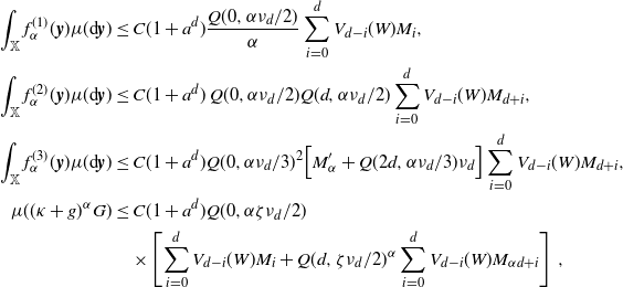 \begin{align}\int_{\mathbb{X}} f_\alpha^{(1)}({\boldsymbol{y}})\mu({\textrm{d}} {\boldsymbol{y}}) &\le C (1+a^d) \frac{Q(0,\alpha \nu_{d}/2)}{\alpha} \sum_{i=0}^d V_{d-i}(W) M_i,\\\int_{\mathbb{X}} f_\alpha^{(2)}({\boldsymbol{y}})\mu({\textrm{d}} {\boldsymbol{y}}) &\le C(1+a^d) \,Q(0,\alpha\nu_{d}/2)Q(d,\alpha\nu_{d}/2) \sum_{i=0}^d V_{d-i}(W) M_{d+i},\\\int_{\mathbb{X}} f_\alpha^{(3)}({\boldsymbol{y}})\mu({\textrm{d}} {\boldsymbol{y}}) &\le C (1+a^d) Q(0,\alpha\nu_{d}/3)^2\Big[M^{\prime}_{\alpha} +Q(2d,\alpha\nu_{d}/3)\nu_{d} \Big] \sum_{i=0}^d V_{d-i}(W) M_{d+i},\\\mu ((\kappa+g)^{\alpha} G) &\le C (1+a^d) Q(0,\alpha \zeta\nu_{d}/2) \\& \quad \times \left[\sum_{i=0}^d V_{d-i}(W) M_i+ Q(d,\zeta\nu_{d}/2)^\alpha \sum_{i=0}^d V_{d-i}(W) M_{\alpha d+i}\right]\,,\end{align}
and
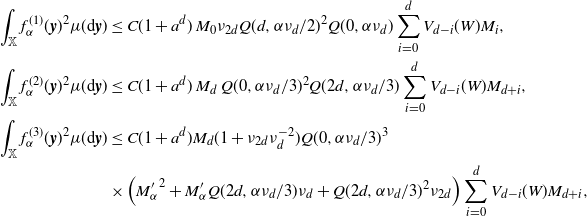 \begin{align}\int_{\mathbb{X}} f_\alpha^{(1)}({\boldsymbol{y}})^2\mu({\textrm{d}} {\boldsymbol{y}}) &\le C (1+a^d) \, M_0 \nu_{2d} Q(d,\alpha\nu_{d}/2)^2 Q(0,\alpha\nu_{d}) \sum_{i=0}^d V_{d-i}(W) M_i,\\\int_{\mathbb{X}} f_\alpha^{(2)}({\boldsymbol{y}})^2\mu({\textrm{d}} {\boldsymbol{y}}) &\le C (1+a^d) \,M_d\,Q(0,\alpha\nu_{d}/3)^2 Q(2d,\alpha\nu_{d}/3) \sum_{i=0}^d V_{d-i}(W) M_{d+i},\\\int_{\mathbb{X}} f_\alpha^{(3)}({\boldsymbol{y}})^2 \mu({\textrm{d}} {\boldsymbol{y}}) &\le C (1+a^d) M_d (1+\nu_{2d}\nu_{d}^{-2})Q(0,\alpha\nu_{d}/3)^3 \\& \times \left({M^{\prime}_{\alpha}}^2+M^{\prime}_{\alpha} Q(2d,\alpha\nu_{d}/3)\nu_{d}+Q(2d,\alpha\nu_{d}/3)^2 \nu_{2d}\right) \sum_{i=0}^d V_{d-i}(W) M_{d+i},\end{align}
where
![]() $C \in (0,\infty)$
is a constant depending only on d.
$C \in (0,\infty)$
is a constant depending only on d.
These modified bounds in combination with the above estimates, along with the fact that
![]() $\nu_{i} \le \nu_{d}^{-1} \nu_{d+i}$
, yield that there exists a constant C depending only on d and
$\nu_{i} \le \nu_{d}^{-1} \nu_{d+i}$
, yield that there exists a constant C depending only on d and
![]() $\tau$
such that for
$\tau$
such that for
![]() $i \in \{1,2,3\}$
,
$i \in \{1,2,3\}$
,
 \begin{equation}\int_{\mathbb{X}} f_{2\beta}^{(i)}({\boldsymbol{y}})\mu({\textrm{d}} {\boldsymbol{y}}) \le C (1+a^d) \nu_{d}^{-\frac{\tau+1}{d+\tau+1}-1}\big(1+\nu_{7d}\nu_{d}^{-7}\big) \sum_{i=0}^d V_{d-i}(W) \nu_{d+i}.\end{equation}
Also, note that by Hölder’s inequality and positive association, for
![]() $i=0, \ldots, d$
, we have
$i=0, \ldots, d$
, we have
Combining this with the estimates above yields that there exists a constant C depending only on d and
![]() $\tau$
such that
$\tau$
such that
 \begin{equation}\mu ((\kappa+g)^{2\beta} G) \le C (1+a^d) \nu_{d}^{-\frac{\tau+1}{d+\tau+1}-1}\big(1+\nu_{7d}\nu_{d}^{-7}\big) \sum_{i=0}^d V_{d-i}(W) \nu_{d+i}.\end{equation}
Arguing similarly, we also obtain that there exists a constant C depending only on d and
![]() $\tau$
such that
$\tau$
such that
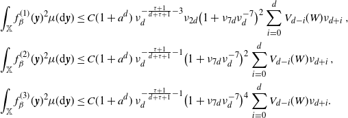 \begin{align}\int_{\mathbb{X}} f_\beta^{(1)}({\boldsymbol{y}})^2\mu({\textrm{d}} {\boldsymbol{y}})&\le C (1+a^d) \, \nu_{d}^{-\frac{\tau+1}{d+\tau+1}-3} \nu_{2d} \big(1+\nu_{7d}\nu_{d}^{-7}\big)^2 \sum_{i=0}^d V_{d-i}(W) \nu_{d+i}\,,\\\int_{\mathbb{X}} f_\beta^{(2)}({\boldsymbol{y}})^2\mu({\textrm{d}} {\boldsymbol{y}}) &\le C (1+a^d) \,\nu_{d}^{-\frac{\tau+1}{d+\tau+1}-1}\big(1+\nu_{7d}\nu_{d}^{-7}\big)^2 \sum_{i=0}^d V_{d-i}(W) \nu_{d+i}\,,\\\int_{\mathbb{X}} f_\beta^{(3)}({\boldsymbol{y}})^2\mu({\textrm{d}} {\boldsymbol{y}}) &\le C (1+a^d) \,\nu_{d}^{-\frac{\tau+1}{d+\tau+1}-1} \big(1+\nu_{7d}\nu_{d}^{-7}\big)^4\sum_{i=0}^d V_{d-i}(W) \nu_{d+i}.\end{align}
Thus, there exists a constant C depending only on d and
![]() $\tau$
such that for
$\tau$
such that for
![]() $i \in \{1,2,3\}$
,
$i \in \{1,2,3\}$
,
 \begin{equation}\int_{\mathbb{X}} f_\beta^{(i)}({\boldsymbol{y}})^2\mu({\textrm{d}} {\boldsymbol{y}}) \le C (1+a^d) \, \nu_{d}^{-\frac{\tau+1}{d+\tau+1}-1} \big(1+\nu_{7d}\nu_{d}^{-7}\big)^4 \sum_{i=0}^d V_{d-i}(W) \nu_{d+i}.\end{equation}
Plugging (4.24), (4.25), and (4.26) into (4.6) and (4.7) and using Proposition 2.1 to lower-bound the variance yields the desired bounds.
Proof of Corollary
2.1. Define the Poisson process
![]() $\eta^{(s)}$
with intensity measure
$\eta^{(s)}$
with intensity measure
![]() $\mu^{(s)}\,:\!=\,\lambda \otimes\theta\otimes\nu^{(s)}$
, where
$\mu^{(s)}\,:\!=\,\lambda \otimes\theta\otimes\nu^{(s)}$
, where
![]() $\nu^{(s)}(A)\,:\!=\,\nu(s^{-1/d}A)$
for all Borel sets A. It is straightforward to see that the set of locations of exposed points of
$\nu^{(s)}(A)\,:\!=\,\nu(s^{-1/d}A)$
for all Borel sets A. It is straightforward to see that the set of locations of exposed points of
![]() $\eta_s$
has the same distribution as that of those of
$\eta_s$
has the same distribution as that of those of
![]() $\eta^{(s)}$
, multiplied by
$\eta^{(s)}$
, multiplied by
![]() $s^{-1/d}$
, i.e., the set
$s^{-1/d}$
, i.e., the set
![]() $\{x \;: \; {\boldsymbol{x}} \in \eta_s \text{ is exposed}\}$
coincides in distribution with
$\{x \;: \; {\boldsymbol{x}} \in \eta_s \text{ is exposed}\}$
coincides in distribution with
![]() $\{s^{-1/d}x \;: \; {\boldsymbol{x}} \in \eta^{(s)} \text{ isexposed}\}$
. Hence, the functional
$\{s^{-1/d}x \;: \; {\boldsymbol{x}} \in \eta^{(s)} \text{ isexposed}\}$
. Hence, the functional
![]() $F(\eta_s)$
has the same distribution as
$F(\eta_s)$
has the same distribution as
![]() $F_{s}(\eta^{(s)})$
, where
$F_{s}(\eta^{(s)})$
, where
![]() $F_{s}$
is defined as in (2.1) for the weight function
$F_{s}$
is defined as in (2.1) for the weight function
with
![]() $W_s\,:\!=\,s^{1/d} W$
. It is easy to check that for
$W_s\,:\!=\,s^{1/d} W$
. It is easy to check that for
![]() $k \in \mathbb{N}$
, the kth moment of
$k \in \mathbb{N}$
, the kth moment of
![]() $\nu^{(s)}$
is given by
$\nu^{(s)}$
is given by
![]() $\nu^{(s)}_k=s^{k/d}\nu_k$
and
$\nu^{(s)}_k=s^{k/d}\nu_k$
and
![]() $\lambda(W_s)=s \lambda(W)$
. We also have
$\lambda(W_s)=s \lambda(W)$
. We also have
 \begin{align}V_{\nu^{(s)}}(W_s)=\sum_{k=0}^d V_{d-i}(s^{1/d} W) \nu_{d+i}^{(s)} = \sum_{k=0}^d s^{\frac{d-i}{d}} V_{d-i}(W) s^{\frac{d+i}{d}}\nu_{d+i }=s^2 V_\nu (W).\end{align}
Finally, noticing that
 \begin{align}l_{a,\tau}(\nu_{d}^{(s)})&=\gamma\left(\frac{\tau+1}{d+\tau+1},a^{d+\tau+1} s\nu_{d} \right) (s\nu_{d})^{-\frac{\tau+1}{d+\tau+1}} \\&\ge \gamma\left(\frac{\tau+1}{d+\tau+1},a^{d+\tau+1} \nu_{d} \right) (s\nu_{d})^{-\frac{\tau+1}{d+\tau+1}}\end{align}
for
![]() $s\geq 1$
, we deduce the result directly from Theorem 2.3. The optimality of the Kolmogorov bound follows from arguing as in the proof of Theorem 2.2.
$s\geq 1$
, we deduce the result directly from Theorem 2.3. The optimality of the Kolmogorov bound follows from arguing as in the proof of Theorem 2.2.
Acknowledgements
We would like to thank Matthias Schulte for raising the idea of extending the central limit theorem to functionals of the birth–growth model with random growth speed. We are grateful to the referees for pointing out connections to other papers and encouraging us to explore an applied motivation for our model. A major part of the work was done when C. B. was employed by the University of Luxembourg.
Funding information
I. M. and R. T. have been supported by the Swiss National Science Foundation Grant No. 200021_175584.
Competing interests
There were no competing interests to declare which arose during the preparation or publication process of this article.


