
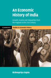

In the year of independence, after 200 years of British rule, India was one of the poorest countries in the world. India was poor not just in comparison to industrialized countries; it was poor even by the standards of other developing countries. Figure 1.1 shows that Latin American countries were richer than countries in Asia and Africa. Latin American countries, such as Brazil, Argentina, and Mexico, had gained independence in the nineteenth century and therefore had designed their own policies for a century. Within Asia, Indian per capita GDP in 1990 International Geary-Khamis dollars was 619 in 1950, compared to 817 in Indonesia, 854 in South Korea, 916 in Taiwan, 1559 in Malaysia, and 1253 in Sri Lanka (see Figure 1.1). Indian GDP per capita was comparable to several countries in Africa in 1950. These countries were among the poorest in the world.
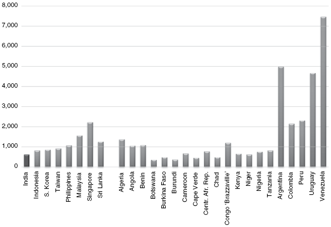
Figure 1.1 Per capita GDP in India and other developing countries (1950) (1990 International Geary-Khamis dollars)
Figure 1.2 shows changes in Asian and Latin American countries between 1910 and 1950. The independent countries in Latin America grew faster, whereas the colonies grew more slowly. In particular India and Indonesia show stagnation.
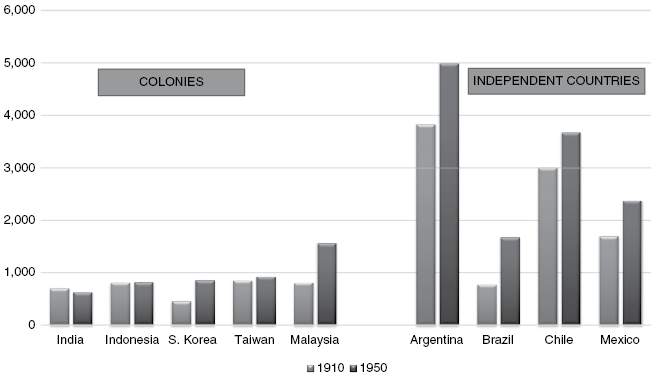
Figure 1.2 Changes in GDP per capita in Asia and Latin America (1910–1950) (1990 International Geary-Khamis dollars)
Colonial rule began with the conquest of Bengal by the East Indian Company in 1757. India formally became a part of the British Empire in 1858 with a transition to Crown rule. Crown rule lasted until 1947. Did the long years of colonial rule impoverish India? Was India prosperous before the conquest by the East India Company? How can we measure prosperity in the seventeenth and eighteenth centuries?
Urbanization is often used as a measure of economic development the further we go back in history. The agricultural surplus needed to sustain cities is a measure of development. City size, city growth, and share of the urban population in a country have been used by economic historians to measure development in the context of Europe, China, and other parts of the world. Historians have suggested that India was more urban in the eighteenth century compared to the end of the nineteenth century (Roy Reference Roy2013, chap. 6). The share of the urban population in India during Akbar’s reign has been estimated at 15 per cent (Habib Reference Habib, Raychaudhuri and Habib1982a). In 1901, the urbanization rate was 10 per cent (Visaria and Visaria Reference Visaria, Visaria and Kumar1983). The sixteenth-century urbanization rate was not attained again until after independence. Did the decline of the urban economy suggest a decline in living standards during colonial rule?
In this chapter I explore another measure of economic development, the changes in GDP per capita. Estimates of GDP per capita for India going back to 1600 are available in the work of Broadberry et al. (Reference Broadberry, Custodis and Gupta2015). They allow a comparison of the average living standard in India across time starting from the reign of Akbar until the end of the nineteenth century. They also make possible comparison with other countries. After the industrial revolution, Britain was the most industrialized economy and also among the most urbanized. This chapter will look at Indian living standard in comparison with that in Britain to understand the timing of the economic divergence between India and Britain. Was the standard of living in Britain before the industrial revolution the same as in India? Did India and Britain have comparable average incomes before colonization? Due to data constraints, it is not possible to use some of the other indicators of economic development, such as life expectancy or literacy, before the late nineteenth century. I will focus on changes in real wages of unskilled urban workers as evidence as this is more easily available and provide evidence on newly estimated GDP per capita to understand the changes in the standard of living in India over four centuries.
I start with qualitative accounts of living conditions followed by quantitative evidence on real wages and estimates of per capita GDP. I evaluate the possible impact of colonial rule in economic decline and stagnation and low per capita GDP. The final section of the chapter offers a historical perspective of the changes in Indian per capita GDP after independence evaluated in the context of available evidence over 400 years.
1.1 What Do We Know: Qualitative and Quantitative Evidence?
The travelogues of Europeans in India in the sixteenth and seventeenth centuries often described the great wealth and opulence of the citizens, but this perspective reflected their narrow exposure to the ruling elites. The ruling elites enjoyed a luxurious lifestyle, enjoying high-quality food, clothing, and ornaments, and living in high-quality housing. This was a great contrast to the rudimentary lifestyle of the common men and women (Chandra Reference Chandra, Raychaudhuri and Habib1982). Moreland, in his book India at the Death of Akbar (Reference Moreland1923), described the luxurious lifestyles of the nobility, who were patrons of the arts and supported scholars, poets, physicians, painters, musicians, and dancers and employed many servants. The wealthier among the middle classes included merchants, money-lenders, and other professional groups who tried to imitate the lifestyles of the nobility. The middle class was small and the merchants that European travellers had contact with enjoyed a comfortable lifestyle (Moreland Reference Moreland1923).
At the same time, most travel accounts of the places outside the urban centres in Mughal India and the Deccan noted that the majority of Indians lived in poverty (Chandra Reference Chandra, Raychaudhuri and Habib1982; Fukazawa Reference Fukazawa, Raychaudhuri and Habib1982). The labouring classes lived in mud huts with thatched roofs, consumed inferior grains, had minimal clothing, and most did not use footwear. Wheat was not widely consumed, even in the wheat producing areas, and inferior grains such as jowar and bajra were grown everywhere (Moreland Reference Moreland1923, pp. 197–203). Pelsaert, a representative of the Dutch East India Company who was in Agra in the early seventeenth century, commented on the contrast between the extravagant luxury of the ruling classes and the poverty of the masses (Thatcher Reference Thatcher1926). Francis Buchanan (Reference Buchanan1807), an employee of the East India Company, conducted surveys in the Bengal and Mysore regions and documented the economic conditions in the first decades of the nineteenth century. Buchanan claimed that, although weavers enjoyed a comfortable lifestyle, the majority of cultivators lived in poverty. Moreland (Reference Moreland1923) confirms that the poverty of the majority was largely unchanged in the early twentieth century.
An assessment of Indian lifestyle by Europeans based on the type of clothing, footwear, and furniture used in their homes reflected the cultural values of the writers and is not an objective assessment. However, information on the type of food consumed and the quality of dwellings provides valuable information to make comparisons possible, despite the cultural prejudice that might have characterized the comments by European travellers. By distinguishing between the lifestyles of the elites and those of the common men and women, these accounts documented the inequality between the rich and the poor.
There exist other sources that come from local observers, but these are relatively rare. Abul Fazl, a member of Akbar’s court who documented the economic conditions during Akbar’s reign, commented on the basic lifestyle of the common people (Chandra Reference Chandra, Raychaudhuri and Habib1982). Analysing temple records in Southern India, Ramaswamy (Reference Ramaswamy1985) confirms a similar picture. There was a prosperous nobility, a small middle class of weavers, and a populous group of rural poor and low-caste artisans. The rich and the middle social classes consumed rice, but others could only afford inferior grain, such as ragi (Ramaswamy Reference Ramaswamy1985, pp. 99–100).
A different view comes from the work of Parthasarathi (Reference Parthasarathi1998, 2011) and Sivramkrishna (Reference Sivramkrishna2009) using evidence from Southern India. Parthasarathi (Reference Parthasarathi1998) compares the living standard of weavers in South India with that of the British weavers in the mid-eighteenth century. Using wages of weavers documented by the East India Company, Parthasarathi finds that, in real terms, they were similar to that of British weavers. More recently, Sivramkrishna (Reference Sivramkrishna2009) used evidence from Buchanan’s survey of Mysore to calculate living standards in terms of the consumption of a cheaper grain, ragi, rather than rice. This comparison suggests that wages in many occupations reflect living standards well above subsistence at the beginning of the nineteenth century, although not at the level of parity with English weavers that Parthasarathi found.
Another indicator of economic development that historians can use in the absence of other systematic data is the relative price of factors of production. Wages as the price of labour indicate the relative abundance or scarcity of labour, and similarly rental cost of capital indicates its scarcity or abundance. Typically, low wages are correlated with lower indicators of economic development. Pelsaert (Reference Pelsaert1925) and Bernier (Reference Bernier1916) refer to the scarcity of capital and cheapness of labour (Habib Reference Habib1969). In all sectors, from palaces and royal courts to services for the nobility, foreigners noted the excess employment relative to Europe, pointing to labour abundance. While European writers spoke of the high quality and skills of the craftsmen, they noted the rudimentary nature of the technology used and the sparing use of metal, indicating that the mining and engineering sectors were underdeveloped. Pelsaert noted with respect to crafts in Agra: ‘For a job which one man would do in Holland, here it passes through four men’s hands before it is finished’ (Habib Reference Habib1969).
Bayly’s (Reference Bagchi1983) description of a thriving market economy in North India during the eighteenth century leaves an impression of a prosperous, mainly urban, commercial sector but says little about the living standards of the vast majority of the population, even in the urban centres. Bayly’s rich account of the vibrancy of markets does not quantify the size of the commercial sector nor its share in GDP and therefore it cannot say much about the representativeness of this sector and how the average Indian lived. While cultural and climatic conditions can explain some of the consumption differences between India and Europe, most qualitative accounts suggest that the average Indian lived in poverty. The image of the prosperous weaver, or the rich nobility, or a vibrant commercial sector did not represent the living standard of the majority of Indians.
1.2 Quantitative Measures of Living Standards
The first accounts using quantitative indicators of living standards come from the work of Shireen Moosvi (Reference Moosvi1973, 1977, 2015) and Najaf Haider (Reference Haider2004) for North India, and Vijaya Ramaswamy (Reference Ramaswamy1985) and Brennig (Reference Brennig1986) for South India. In their research spanning decades, Irfan Habib and Shireen Moosvi methodically documented the economic markers in Mughal India, from wages, prices, and interest rates to agricultural productivity and fiscal capacity. The first step for building time series evidence can be found in Mukherjee’s (1967) estimates of real wages from 1600. The book puts together data on wages and prices from different parts of the country, so that real wages can be calculated at the regional level. Broadberry and Gupta (Reference Broadberry and Gupta2006) took a further step to construct silver and grain wages for North and South India, using systematic evidence of wages and prices from different sources for all regions of India. This made it possible to compare long-run development of the Indian economy with that of other countries.
The starting point is 1595, in India under Akbar. Wages from different occupations were documented in Abul Fazl (1595) Ā’ īn–i-Akbarī and can be classified into skilled and unskilled wages. This is a reference point for real wage comparisons over the next centuries. Desai (Reference Desai1972) claimed that, at best, the average standard of living in 1961 was no higher than in 1595 in Mughal India. The average wage during Akbar’s reign would buy fewer industrial goods, such as clothing, but it could buy more food, given the relative prices between agriculture and industry in the sixteenth century. The average wage in 1961 could buy less food but more cloth than the average wage in 1595. (Desai, Reference Desai1972) while this comparison was useful in assessing Indian living standards soon after independence with pre-colonial Mughal India, it did not say anything about the intervening centuries. When did the decline begin? Did colonization contribute to the real wage decline and stagnation over the centuries or did the decline begin before the conquest of Bengal by the East India Company?
Mukherjee (Reference Mukherjee1967) found a downward trend in real wages during the seventeenth and eighteenth centuries, before recovering during the twentieth century. Based on evidence from 1595 and other archival and secondary sources for the seventeenth, eighteenth, and nineteenth centuries, Broadberry and Gupta (Reference Broadberry and Gupta2006) constructed a wage series over this period for northern, western, and southern India. Using prices of the staple foods, such as rice or wheat, depending on the region, and a representative selection of wages from different regions for unskilled and skilled workers, they constructed a series for money wages and grain wages. Money wages show the nominal value of wage and the grain wage computes the purchasing power of the wage in terms of food grains. This data can be used to establish not only the trend in living standards over the centuries, but also what Indian living standards might have looked like relative to the prosperous societies of Northwest Europe (Table 1.1).
Table 1.1 Indian silver and grain wages (1595–1874)
| (A) Northern and western India | ||||||
|---|---|---|---|---|---|---|
| Silver wage (grams per day) | Wheat grain wage (kg per day) | Rice grain wage (kg per day) | ||||
| Unskilled | Skilled | Unskilled | Skilled | Unskilled | Skilled | |
| 1595 | 0.67 | 1.62 | 5.2 | 12.6 | 3.1 | 7.5 |
| 1616 | 0.86 | 3.0 | 2.4 | |||
| 1623 | 1.08 | 3.8 | 2.9 | |||
| 1637 | 1.08 | 2.37 | 3.8 | 8.3 | 2.9 | 6.5 |
| 1640 | 1.29 | 4.5 | 3.5 | |||
| 1690 | 1.40 | 4.3 | ||||
| 1874 | 1.79 | 5.27 | 2.5 | 7.5 | ||
| (B) Southern India | ||||
|---|---|---|---|---|
| Silver wage (grams per day) | Rice grain wage (kg per day) | |||
| Unskilled | Skilled | Unskilled | Skilled | |
| 1610–13 | 1.15 | 5.7 | ||
| 1600–50 | 1.15 | 3.2 | ||
| 1680 | 1.44 | 2.44 | 3.9 | 6.9 |
| 1741–50 | 1.49 | 2.1 | ||
| 1750 | (3.02)* | (7.56)* | (4.2)* | (10.5)* |
| 1779 | 0.86 | 1.1 | ||
| 1790 | 1.44 | 1.8 | ||
Note: * These figures come from Parthasarathi (Reference Parthasarathi1998) and are outliers compared to the rest of the series. These wages may have been isolated cases of high-skilled weavers
1.3 Silver Wage and Grain Wage
The simplest way to think of grain wage is how much food the money wage of a typical unskilled worker would buy. A similar calculation can be made for a typical skilled worker. The grain wage of an unskilled worker proxies the lowest wages in the economy and is therefore a good measure of the average living standard. The difference between wages of skilled and unskilled workers is also indicative of the skill premia in the economy and the relative shortage of skilled workers and therefore the level of economic development measured in terms of human capital.
The established practice in the literature for measuring living standards in Europe across time and place has been to gather data on money wages of unskilled and skilled workers and convert these to a common unit of grams of silver. This gives us the silver wage. Converting money wages in various currencies to a silver standard makes international comparisons possible. The silver wage is then divided by the silver price of the common local grain. This would give us the grain wage, a crude but common measure of the standard of living. If prices of non-food items in consumption are not available, then measuring the purchasing power of wage in terms of grain price is a reasonable approximation of real wage in subsistence economies. The closer an economy is to subsistence, the more accurate is the grain wage as a measure of living standards, since a large part of the income is spent on basic foods for survival. The more industrial an economy, the more diversified is the consumption basket. It contains more processed foods and industrial products. If we do not consider a suitable consumption basket, this would bias the grain wage. However, during the period of the comparison in this chapter, most economies were close to subsistence and therefore grain wage is a good approximation of real wage. This method has been applied to India by Broadberry and Gupta (Reference Broadberry and Gupta2006).
Part A of Table 1.1 shows silver wages and grain wages in northern and western India, drawing largely on sources for Agra and Surat. Note that these are urban wages and there is little information on rural wages. Grain wages in northern and western India are obtained by dividing the silver wages by the price of wheat, the main grain produced in the region, expressed in terms of silver. Although the silver wages rose between 1595 and 1874, grain wages declined in northern and western India as money wages failed to keep up with rising grain prices.
Data for southern India is in part B of Table 1.1. The wage and price data are largely from the area around Madras and in many cases are the wages of skilled and unskilled workers in textile weaving. Money wage rates here are available in pagoda units, a gold coin, and are converted to silver rupees using East India Company’s standard rates from Chaudhuri (Reference Chaudhuri1978). Silver wages for Southern India are then converted to grain wages using the price of rice, the main grain consumed in the region, as the deflator. Overall, the levels and trends of silver and grain wages in Southern India fit well with the levels and trends in the North, except in 1750. As explained in the note Figure 1.1, these particular wages are outliers.
To make any normative statement about the standard of living, we need to have a measure of the subsistence level. Brennig (Reference Brennig1986) argues that subsistence consumption for a household of six was 3.1 kg of rice per day. The wheat/rice ratio of calories per lb gives the calorie equivalence of 4.7 kg of wheat per day for a family of six (Parthasarathi Reference Parthasarathi1998, p. 83). On this basis, grain wages were always above subsistence for skilled workers but fell below the subsistence level for unskilled workers during the seventeenth century. This raises the question: how did the families of unskilled labourers survive? The evidence suggests that, although we use the price of rice and wheat as the deflator, poorer families tended to consume mainly cheaper grains such as ragi, as discussed by Sivramkrishna (Reference Sivramkrishna2009). Rice and wheat prices are used because the market price of these goods is recorded more systematically. Therefore, the tables capture the declining trend in grain wage rather than suggesting that people lived below the subsistence level.
Table 1.2 provides a comparison of silver and grain wages for unskilled labourers in England and India. Part A shows that Indian silver wages for unskilled workers were little more than one-fifth of the English level in the late sixteenth century and fell to just over one-seventh of the English level during the eighteenth century. Part B of Table 1.2, the grain wage, shows that India remained closer to the English level until the end of the seventeenth century. The data indicates a sharp divergence during the eighteenth century, partly due to a rise in the English grain wage, and partly due to a decline in the Indian grain wage. Table 1.1 shows the decline in Indian living standards, from a high point in 1595 for northern India and in 1610 for Southern India. Table 1.2 illustrates the timing of the Great Divergence. The grain wage declined from 80 to 95 per cent of the British wage to less than 30 per cent by the middle of the nineteenth century. The table also shows that the decline began well before colonization.
Table 1.2 An England–India comparison of the daily wages of unskilled labourers (1550–1849)
| (A) Silver wages (grams of silver per day) | |||
|---|---|---|---|
| Date | Southern England | India | Indian wage as a % of English wage |
| 1550–99 | 3.4 | 0.7 | 21 |
| 1600–49 | 4.1 | 1.1 | 27 |
| 1650–99 | 5.6 | 1.4 | 25 |
| 1700–49 | 7.0 | 1.5 | 21 |
| 1750–99 | 8.3 | 1.2 | 14 |
| 1800–49 | 14.6 | 1.8 | 12 |
| (B) Grain wages (kilograms of grain per day) | ||||
|---|---|---|---|---|
| Date | India | Indian wage as a % of English wage | ||
| England | (wheat) | (rice, on wheat equivalent basis) | ||
| (wheat) | ||||
| 1550–99 | 6.3 | 5.2 | 83 | |
| 1600–49 | 4.0 | 3.8 | 95 | |
| 1650–99 | 5.4 | 4.3 | 80 | |
| 1700–49 | 8.0 | 3.2 | 40 | |
| 1750–99 | 7.0 | 2.3 | 33 | |
| 1800–49 | 8.6 | 2.5 | 29 | |
I noted that grain wage is a crude approximation of living standards and therefore has two limitations. As stated before, it is more accurate at low levels of economic development when grain accounts for a very large share of consumption. Another concern is that grain wage is calculated mainly with urban wages and prices and gives a biased view for economies that are agricultural. In the following section I will discuss the refinements that have been introduced in estimating real wages.
1.4 Real Consumption Wages and Welfare Ratios
The first step towards a different measure of consumption is to introduce a cloth wage. The simplest consumption basket consists of grain and cloth. Historical prices of cloth and grain are more easily available than for many other goods. The cloth wage is constructed by systematically collecting evidence on the price of cotton cloth in India from the records of the East India Company for the period before 1833 and from Parliamentary Papers for subsequent years (Broadberry and Gupta Reference Broadberry, Gupta, Chaudhary, Gupta, Roy and Swamy2015). The cloth wage represents the amount of cloth the silver wage would buy and indicates that changes in the relative price of cloth and grain that can affect consumption of cloth. A basic subsistence basket includes both grain and cloth and therefore a weighted average of the grain wage and the cloth wage would be a better measure of a real consumption wage. Consumers’ budgets during this period (Allen Reference Allen, Hatton, O’Rourke and Taylor2007; Buchanan Reference Buchanan1807) typically shows that consumers spent two-thirds on grain. The typical consumption basket is more diversified, but a consumption wage using basic shares of grain and cloth is a good approximation of the real wage when prices of all commodities are not available systematically.
Figure 1.3 presents these different measures of living standards: the grain wage, the cloth wage and the real consumption wage using a weighted average of grain and cloth. The cloth wage started at a lower level, did not change much during the seventeenth and eighteenth centuries, and increased substantially during the nineteenth century. This reflects the change in the price of cloth relative to the price of grain. The turning point came in 1851 with the arrival of cheaper, machine-made cloth from Britain. Cloth consumption per capita increased from the second half of the nineteenth century. This is in line with the evidence from Desai (Reference Desai1972) a century later that the average wage in 1961 could have bought less food but more cloth than the average wage in 1595. As Figure 1.3 shows, the grain wage in 1871 was half of what it was in 1595, the cloth wage rose, and the real consumption wage declined (although less than the grain wage) and rose in the nineteenth century.
Figure 1.3 Grain wage, cloth wage, and consumption wage (1600–1871): 1871=100
What did the actual consumption basket of an unskilled worker in the seventeenth century look like? Allen (Reference Allen, Hatton, O’Rourke and Taylor2007) constructed a consumption basket for northern India and Bengal that included a variety of food items such as the basic grain, usually rice or millet, and other comparable foods using the items that were common in a basic European basket of this period, and non-food, such as cloth.
Allen (Reference Allen, Hatton, O’Rourke and Taylor2007) went on to construct welfare ratios, defined as the number of consumption baskets that can be purchased with the average annual earnings of a wage labourer using that country’s typical subsistence consumption basket. A welfare ratio above one indicates that wages are sufficient for a society to feed itself. Allen (Reference Allen, Hatton, O’Rourke and Taylor2007) compares living standards in England and India by introducing the concept of a European respectability consumption basket. This included grain, bread, beans, cheese, meat, eggs, butter, beer, linen, candles, lamp oil, and fuel. British workers enjoyed a welfare ratio of one or above. Using a basket that included equivalent consumption items in the Indian context, Allen found that the welfare ratio for India was always below one, except in 1600. Table 1.3 shows Allen’s bare-bones subsistence consumption baskets for India based on rice, the superior grain, and millet, an inferior grain. The welfare ratios calculated using the bare-bones subsistence basket rarely fell below one.
Table 1.3 Allen’s bare-bones consumption basket for India
| The basket | Rice-based consumption | Millet-based consumption | ||||
|---|---|---|---|---|---|---|
| Quantity per year | Nutrition per person | Quantity per year | Nutrition per person | |||
| Kilogram | Calories | Protein | Kilogram | Calories | Protein | |
| Rice | 164 | 1627 | 34 | |||
| Millet | 209 | 1731 | 63 | |||
| Beans | 20 | 199 | 11 | 10 | 100 | 5 |
| Meat | 3 | 21 | 1 | 3 | 21 | 1 |
| Ghi | 3 | 72 | 0 | 3 | 72 | 0 |
| Sugar | 2 | 21 | 0 | 2 | 21 | 0 |
| Cotton cloth | 3 metres | 3 metres | ||||
| Total | 1940 | 46 | 1945 | 69 | ||
Allen’s (2007) international comparison of real consumption wages between England and India broadly confirms the grain wage findings of Broadberry and Gupta (Reference Broadberry and Gupta2006). Real consumption wages in North India and Bengal were close to the English level in the early seventeenth century but fell substantially behind during the eighteenth century.
There is evidence on the actual consumption basket from Bengal and Mysore from Buchanan’s survey of the 1810s. This basket gives us a glimpse into the lifestyle of the poorest people from a few districts in Bengal in the early nineteenth century. Eighty per cent of the consumer expenditure was on food, which included coarse rice, lentils, oil, and salt. All fish, meat, and fuel were gathered, not bought in the market (Buchanan’s survey of Dinajpur, 1833, pp. 149–150). Other evidence from the survey shows that most of the expenditure was on food for labourers, with minimal expenditure on dwellings and clothing and some expenditure on religious ceremonies. A comparable expenditure pattern was observed in surveys of the consumption of Bombay cotton mill workers in the 1920s.
The unskilled workers were relatively better off in India under Akbar, according to the indicators of grain wage, consumption wage, and Allen’s welfare ratio, than at the end of colonial rule. The decline in the grain wage during the seventeenth and eighteenth centuries was accompanied by an increase in population from 142 million in 1600 to 207 million in 1801 (Visaria and Visaria Reference Visaria, Visaria and Kumar1983, p. 466). Grain wage stagnated as the population rose further to 256 million in 1871, but the growth rate of population was not high. Periodic famines created spikes in grain prices, sometimes with devastating consequences for mortality, until the beginning of the twentieth century (Broadberry and Gupta Reference Broadberry, Gupta, Chaudhary, Gupta, Roy and Swamy2015). The main decline in grain wage occurred in the seventeenth and eighteenth centuries. As Figure 1.4 shows, most of the nineteenth century saw stagnation. While Akbar’s reign was the high point in living standards, the decline began well before colonization and coincided with the rising trade in textiles and the decline of the Mughal Empire.
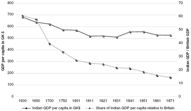
Figure 1.4 Absolute and relative decline of Indian GDP per capita (1600–1871)
1.5 From Wages to Per Capita Income: Historical National Accounting
So far, this is a picture of Indian economic performance before 1871 based on wages and prices. One limitation of wages is that most wages are from non-agricultural activities, while most of the population in India was engaged in agriculture. Therefore, a full assessment of living standard requires information on the population engaged in agriculture. This requires us to move from wages to GDP per capita, which is a challenging task going back in history.
To estimate GDP for India over several centuries, Broadberry, Custodis, and Gupta (Reference Bogart, Chaudhary, Chaudhary, Gupta, Roy and Swamy2015) followed the historical national accounting methodology that has been used to estimate GDP for several European countries and increasingly for countries outside Europe. The method builds demand side estimates of sectoral output for a given population on the basis of what is needed for subsistence. The estimates are then revised based on income elasticity of demand using information on wages. The robustness of the demand side estimates come from cross-checks with supply side estimates of sectoral output at given points in time for which information is available. Broadberry et al. (Reference Broadberry, Custodis and Gupta2015) used this methodology to have demand side estimates with the currently available Indian data on population and consumption, and the series analysed earlier on wages, grain prices, and cloth prices. The estimation used data on agricultural and industrial exports, crop yields and cultivated acreage, cloth consumption per capita, urbanization rates, and government revenue to build up to aggregate output for agriculture, industry, and services from the supply side in benchmark years. This provides the first systematic long-run estimates of GDP per capita, challenging Angus Maddison’s estimates that started in 1000 CE. Maddison assumed that most economies were at subsistence and therefore his estimates of Indian GDP per capita show no change until modern economic growth in the twentieth century. The new estimates are based on careful analysis of available statistical evidence and show changes over the centuries.
In Table 1.4, agricultural output is constructed from the demand side using data on population, wages, and prices to estimate domestic demand and data on exports for foreign demand. These demand-based estimates are then cross-checked with agricultural supply, estimated using data on crop yields and the cultivated land area. Industrial production for the domestic market can also be estimated from information on wages and prices and cross-checked against independent information on cloth consumption per capita. Output of the export industries is based on the export data collected by the European East India Companies. A weighted average of the output of home and export industries is used to estimate changes in industry and commerce. For services, the output of the government sector is measured using data on tax revenue, while the size of the private services and the rent sector is assumed to move in line with the urban population. The cross-checks, where possible, match estimated agricultural output from the supply and demand sides and the estimation of home industrial output matches with independent estimates of cloth consumption per head.
Table 1.4 Changes in GDP by sector (1600–1871) (1871=100)
| Year | Agriculture | Industry and commerce | Rent and services | Government | Total output | Per capita GDP |
|---|---|---|---|---|---|---|
| 1600 | 67.8 | 80.0 | 95.5 | 84.3 | 71.9 | 129.7 |
| 1650 | 63.8 | 75.3 | 95.5 | 48.2 | 67.3 | 121.2 |
| 1700 | 72.2 | 87.0 | 103.0 | 60.4 | 75.7 | 118.2 |
| 1750 | 76.8 | 97.0 | 110.8 | 46.9 | 81.3 | 109.6 |
| 1801 | 79.3 | 127.0 | 120.7 | 74.5 | 87.5 | 108.2 |
| 1811 | 76.0 | 104.6 | 125.3 | 77.3 | 82.9 | 98.8 |
| 1821 | 72.9 | 89.0 | 110.3 | 70.6 | 79.2 | 98.9 |
| 1831 | 77.5 | 82.4 | 116.2 | 71.3 | 81.8 | 97.0 |
| 1841 | 82.8 | 92.9 | 104.6 | 79.3 | 87.3 | 105.5 |
| 1851 | 91.5 | 99.6 | 114.4 | 87.8 | 95.9 | 105.8 |
| 1861 | 89.2 | 107.3 | 109.4 | 86.9 | 95.6 | 100.3 |
| 1871 | 100 | 100 | 100 | 100 | 100 | 100.0 |
Table 1.4 shows that total industry and commerce grew rapidly between 1650 and 1801. This sector includes home industry and export industry. The latter grew faster in the seventeenth and eighteenth centuries as Figure 1.5 shows, driven by exports of cotton cloth. This industry grew rapidly as European trading companies traded in cotton cloth that dominated the international market. The decline of this industry in the nineteenth century, when British cotton textiles flooded the Indian market, is known as deindustrialization. The agricultural sector grew, but more slowly. Total output or GDP growth, although positive, failed to keep pace with a slow growth in population during this period. This is shown in the last column. The index of per capita GDP is then converted into 1990 International Geary-Khamis dollars to get comparable estimates to British GDP per capita. As Table 1.5 shows, in 1600 Indian GDP per capita was just over 60 per cent of the British level, but by 1871 it had declined to under 15 per cent.
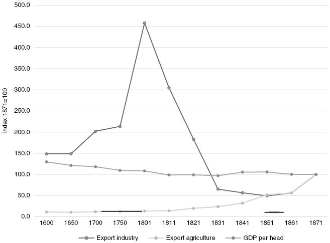
Figure 1.5 Industrial and agricultural exports per capita relative to GDP per capita (1871=100)
Table 1.5 Indian and British GDP per capita (1600–1871) (1990 International Geary-Khamis dollars)
| Year | Indian GDP per capita | British GDP per capita | Indian GDP per capita/ British GDP per capita (%) |
|---|---|---|---|
| 1600 | 682 | 1,123 | 61 |
| 1650 | 638 | 1,100 | 58 |
| 1700 | 622 | 1,563 | 40 |
| 1750 | 576 | 1,710 | 36 |
| 1801 | 569 | 2,083 | 27 |
| 1811 | 519 | 2,065 | 25 |
| 1821 | 520 | 2,133 | 24 |
| 1831 | 510 | 2,349 | 22 |
| 1841 | 555 | 2,613 | 21 |
| 1851 | 556 | 2,997 | 19 |
| 1861 | 528 | 3,311 | 16 |
| 1871 | 526 | 3,657 | 14 |
The timeline of this decline is shown in Figure 1.5. As the blue line shows, India’s per capita GDP declined from a high point in 1600, when it was well above Maddison’s subsistence level per capita GDP of $550 (1990 International Geary-Khamis dollars). By the early nineteenth century, the level was close to that estimated by Maddison. India’s relative decline with respect to Britain was in part due to the absolute decline of Indian living standards and in part due to Britain’s growing prosperity. The new estimates of GDP per capita by Broadberry et al. (Reference Broadberry, Custodis and Gupta2015) confirm the findings based on the wage data that the gap in living standards between India and Britain was relatively small during Akbar’s reign. The decline began during the next phase of the Mughal Empire and continued under the first decades of East India Company rule. The nineteenth century saw stagnation rather than decline with short periods of economic growth that were not sustained.
The phenomenal rise in industrial exports from India, as shown in Figure 1.5, had a small effect on GDP because industry was a small part of the economy. Indian economic growth was largely driven by agriculture, the largest sector. This is shown in Figure 1.6. The trend GDP per capita did not track the changes in exports per capita in industry and agriculture. While industrial exports per capita rose sharply, this was not reflected in GDP per capita. Instead GDP per capita tracked agricultural output per capita all the way up to 1871.
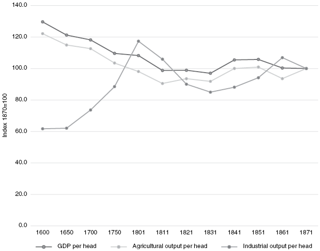
Figure 1.6 Agricultural and industrial output per capita relative to GDP per capita (1871=100)
As Table 1.5 shows, the beginning of the Great Divergence can be traced back to the seventeenth century. Indian GDP per capita declined relative to Britain, but also relative to its high point in 1600. Contrary to the view that the golden age of textile exports from India to the rest of the world had made the country prosperous, this chapter has shown that there was economic decline in the seventeenth and eighteenth centuries. The political aspects of the decline in the seventeenth and eighteenth centuries have been explored, but more research is needed to understand the economic decline of this period. One possible explanation is that most of the fertile plains were already densely populated and as populations moved out of this area, the marginal land was less fertile and produced less output per head. Without more extensive irrigation and better technology, agricultural output could not keep pace with population growth. The declining trend in GDP per capita during the seventeenth and eighteenth centuries occurred in China as well as India. In both countries, this was driven mainly by trends in agriculture, as population growth outstripped the growth in cultivated land area and crop yields did not increase sufficiently to offset the decline in the land-labour ratio.
1.6 Globalization and Stagnation: Economic Performance 1860 to 1947
From 1871 there are systematic annual estimates of GDP by Alan Heston (Reference Heston, Kumar and Desai1983) covering 1870–1900 and Sivasubramonian (Reference Sivasubramonian2000) from 1900 to 2000. These studies have been conducted within a national accounting framework, drawing on the wider availability of statistical information from the beginning of Crown rule. From Table 1.6, we can observe short periods of growth in GDP per capita during the late nineteenth century. From the turn of the twentieth century GDP per capita stagnated and since 1950 it has grown, indicating a transition to sustained economic growth. The Indian economy grew faster than the historical trend but has lagged behind more successful East Asian countries. However, East Asia was an exception among countries emerging from colonization. I will return to this in Chapter 6. The stagnation of Indian incomes and living standards over 100 years of Crown rule points to a failure of colonial policies to generate modern economic growth. Although India became more integrated into the trading world of the British Empire and could have access to the British capital market, the stagnation was driven by stagnation in agriculture, as I will discuss in Chapter 2. The literature has emphasized the decline of the indigenous textile sector as a cause of economic decline in the nineteenth century. This impacted on communities engaged in this sector. Its effect on average living standards was small because the industrial sector was a small part of the economy, as I have argued in this chapter.
Table 1.6 Economic growth in the long run (% per year)
| Per capita income | |
|---|---|
| 1870–1885* | 0.5 |
| 1885–1900* | 0.8 |
| 1900–1947 | 0.1 |
| 1950–1980 | 1.4 |
| 1980–1990 | 3.0 |
| 1990–2000 | 4.1 |
Why did a globalized economy fall into stagnation? Was the integration of India into the global network of the British Empire harmful to economic growth? By the middle of the nineteenth century, Britain had abolished the Corn Laws that imposed tariffs on grain imports and adopted the doctrine of free trade, a policy that suited Britain’s industrial specialization and demand for imported raw materials for the industrial sector. Free trade was imposed on India and other colonies. It is not clear that free trade was the appropriate policy for India at this time, when most countries, including the USA and Germany, were using tariffs to industrialize and grow. The data points to some growth of the Indian economy between 1870 and 1900, when India integrated into the global trading network of the British Empire, but this was short-lived. (see Table 1.6).
The effect of trade on growth, and the differential effect of trade on producers of agricultural and producers of manufactured goods, are debated issues. Theories of trade based on comparative advantage can be applied to colonial trade. Both countries could gain by specializing in the production of goods that could be produced more efficiently. The colonies specialized in agricultural goods and the imperial countries specialized in industrial goods. The colonies gained from the growing demand for food and raw material in the industrial countries and saw rising incomes. The Prebisch–Singer thesis cautioned against this by showing empirically that the terms of trade of agricultural products relative to industrial products declined from the middle of the nineteenth century to the middle of the twentieth century and argued that specialization in agricultural production was not beneficial for economic development (Singer Reference Singer1989). In reality, the nineteenth century saw divergence in living standards between agricultural and industrial countries, with a few exceptions (Findlay and O’Rourke Reference Findlay and O’Rourke2009, p. 415). Cross-country data from the second half of the twentieth century finds a positive effect of trade on per capita GDP (Frankel and Romer Reference Frankel and Romer1999). However, the evidence from the nineteenth century is mixed. Mitchener and Weidenmier (Reference Mitchener and Weidenmier2008) show that being part of an empire increased the volume of trade compared to countries outside the empire. Pascali (Reference Pascali2017) uses cross-country data to show that, for colonies, trade did not always have a positive effect on indicators of economic development. Countries with good institutions benefitted from trade, but others did not and trade may have contributed to the increasing divergence between developed and underdeveloped economies. Therefore, even without considering implications of terms of trade, trade did not necessarily lead to higher incomes in the nineteenth century.
As India integrated into the world economy, trade, investment, and migration rose. The trade–GDP ratio increased dramatically, from 2 to 3 per cent in the mid-1800s to 20 per cent on the eve of the First World War (see Table 1.7). India received 8 per cent of British overseas investment during 1865–1914 (Gupta Reference Gupta, Broadberry and Fukao2021). This was not sufficient to raise the rate of gross capital formation above 7 per cent of GDP. Most of this investment went to the railways.
Table 1.7 Share of trade in income: from colonial times to independent India (%)
| Year | Trade/GDP |
|---|---|
| 1835* | 1.1–2.4 |
| 1857* | 3.6–4.8 |
| 1913* | >20 |
| 1950–1960 | 6.8 |
| 1960–1970 | 5.2 |
| 1970–1980 | 6.0 |
| 1980–1990 | 7.0 |
| 1990–2000 | 10.0 |
The nationalist historians have argued that the railways integrated the agricultural hinterland and the ports, and paved the way for a rising volume of trade in agricultural goods that supported industrial Britain’s demand for food and raw material. I have argued that, despite rising trade, the effect on economic growth was small. This is consistent with Pascali’s (2017) argument that not all countries gained from trade in the first period of globalization. Britain enjoyed a positive trade balance with India. India imported more from Britain than from the rest of the world and exported less to Britain compared to the rest of the world. India’s net exports were positive all through this period, but net exports to Britain turned negative from the 1870s (Gupta Reference Gupta2018). During the interwar years, India’s trade with Britain became more concentrated with the policy of Imperial Preference. Differential tariffs benefitted Britain at the cost of other trading partners (Arthi et al. Reference Arthi, Lampe, Nair and O’Rourke2024).
Figure 1.7 shows an increasing divergence between Britain and Indian per capita GDP over the colonial period. The divergence increased during the first half of the twentieth century as British income increased and Indian income stagnated. As discussed in this section, integration into the global economy of the British Empire did not increase the investment rate or have a significant effect on growth. Stagnation in per capita GDP paralleled agricultural stagnation in the first half of the twentieth century. This will be discussed in Chapter 2.
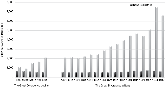
Figure 1.7 The Great Divergence between India and Britain (1600–1947)
1.7 Stagnation to Modern Economic Growth: From Free Trade to Regulation
In 1947, the newly independent state of India moved away from the colonial policies. The first step was to set out an agenda for industrialization and break with the global economy. Global integration and the specialization in agriculture was seen as a hindrance to economic development. This view was expressed in other parts of the underdeveloped world too. The Economic Commission of Latin America, under Raul Prebisch, raised similar concerns. The newly independent states of South Korea and Taiwan adopted industrialization as a goal. Newly independent states in Africa moved in a similar direction a decade later.
To the policymakers in the less developed countries, an open economy was a part of the imperial connection, and an international division of labour based on comparative advantage had adverse consequences on economic development. Industrialization was the way to change this division of labour. While national prestige and tariffs to protect an infant industry had motivated economic policy towards industrialization in nineteenth century Europe and the USA, the rhetoric in post-colonial countries was to break with their imperial connection and move away from specialization in agriculture. The policies for industrialization adopted in the twentieth century were far more interventionist. In the industrialization of Japan and the Soviet Union in the first half of the twentieth century, the state had played a more important role. After 1945, policy makers in Latin America adopted import-substituting industrialization as the goal. Countries gaining independence from colonial rule in Asia and Africa followed a similar path. Import-substituting industrialization was the path of economic development in the less developed world in the 1950s and 1960s. In the short term it raised the rate of growth in many countries. The outcome in the medium and long term, depended on how countries reoriented their policies to reintegrate into the global economy. Newly independent countries in East Asia, such as South Korea and Taiwan, initially followed policies of import-substituting industrialization and regulated international trade. East Asian countries embraced the Japanese model and moved quickly towards reintegration with the international market. Many import-substituting economies, including India, remained protectionist, with adverse consequences on growth.
The vision of Jawaharlal Nehru, India’s first prime minister, was industrialization and self-sufficiency not global connections. Industrial development was at the core of this policy. India moved from being an open economy to one of the most regulated economies in the world. GDP per capita grew at less than 2 per cent per year, which was low in comparison to the fast-growing economies in East Asia. In comparison with other developing countries, India was not that different. Delong (Reference Delong and Rodrik2003) sees India’s performance under planning as average rather than disastrous. Output per worker and the share of investment in GDP was comparable to the average developing country during the period 1960–1992.
The new government introduced Soviet-style five-year plans that set targets for different sectors, regulated international trade, restricted the entry of the private sector into certain industries, and put the public sector in control of the development of intermediate and capital goods industries. A full discussion of the successes and failures of this policy will be taken up in the next chapters. At this point, it is worth noting that the increase in economic growth was due to rising agricultural growth and rapid industrial growth in the early phase of import-substituting industrialization. The policies of state-directed development pulled India out of stagnation, but did not turn it into a high-growth economy.
The country faced several economic and political crises in the 1960s and 1970s. The monsoons failed in 1965 and 1966 with a consequent fall in grain output by 10–20 per cent and India turned to the USA for food aid, which undermined the policy of self-reliance. American food assistance came with the demand for a devaluation of the rupee to ensure greater integration with the global economy. The lack of adequate export earnings showed the vulnerability of inward-looking developmental policies and industrial growth based on import substitution began to slow down. The country did not have enough foreign exchange reserves to pay for food imports. The crisis saw a change in the direction of policies towards agriculture. Infrastructure and subsidized inputs to facilitate adoption of high yielding varieties of seeds paved the way towards the Green Revolution. Chapter 2 will discuss these changes and their implications in more detail.
The political crises that followed changed the nature of Indian politics. The Congress-led government under Nehru had commanded support in all parts of the country. With Nehru’s death in 1964, the political leadership passed on to Lal Bahadur Shastri as prime minister. Shastri’s untimely death in 1968 created a vacuum in leadership and Nehru’s daughter, Indira Gandhi, became prime minister. She did not have the same support. The Congress Party split into two groups. Gandhi built her own brand of socialist developmental policies by nationalizing Indian banks in 1969 and removing the privy purse that the rulers of the princely states enjoyed as a compensation for giving up territorial sovereignty of the regions they had ruled at the time of independence. Gandhi invoked the rhetoric of ‘get rid of poverty’ and signalled redistribution from the privileged to the poor. In reality, Gandhi centralized political power and in 1975 suspended the carefully built democratic institutions of the country.
The 1970s brought further political crisis. The Green Revolution in agriculture had created a strong agricultural lobby whose interests were different to that of industry. New political parties representing agricultural interests demanded more subsidies towards agriculture and different economic policies. The new political groups fragmented the political space and weakened the dominant position of the Congress. When Gandhi called elections in 1977, she was defeated. Indian politics had changed forever from being dominated by the Congress to several regional political parties dominant in the provinces, creating more political competition on the national stage. A number of regional and group-based parties held the balance of power and short-lived coalitions were in government until Gandhi’s re-election in 1980.
In the new regime, the focus of economic policy turned from redistribution to growth. The years leading to the assassination of Indira Gandhi in 1984 and the election of Rajiv Gandhi as prime minister saw a new direction in policy making. From state-directed development in the first three decades after independence, economic policy signalled a greater role to the private sector. The first step was the dismantling of industrial regulation and a gradual removal of industrial licensing. Second, the extensive quantitative controls of trade, such as import quotas, were replaced with price-based controls such as tariffs and subsidies. Both policies opened up opportunities for the private sector, that had previously faced barriers to entry in several industries.
Rodrik and Subramanian (Reference Rodrik and Subramaniam2005) and Kohli (Reference Kohli2006) distinguish between the ‘pro-business’ reforms of the 1980s, when the regulatory framework towards private investment was relaxed, and the ‘pro-market’ reforms that followed a large devaluation of the Indian rupee in 1991. Rodrik and Subramanian (Reference Rodrik and Subramaniam2005) see the removal of industrial licenses and price controls as indicative of an ‘attitudinal shift’ towards the private sector. Private investment was given access to new sectors and faced a favourable environment. The ‘pro-market’ changes, on the other hand, were indicative of opening up the economy to international competition. Rodrik and Subramanian (Reference Rodrik and Subramaniam2005) argue that, during the years of planned industrialization, the Indian economy was at some distance from its potential and the new environment created favourable conditions for existing firms in the private sector and led to a large increase in productivity.
Growth in output per worker increased from 1.3 per cent per year during 1960–1980 to 3.7 per cent per year during 1980–2004. Total factor productivity growth increased from 0.2 per cent to 2.0 per cent per year (Bosworth et al. Reference Bosworth, Collins, Virmani, Collins, Bosworth and Panagariya2007). The pro-market reforms of the 1990s lowered price-based controls and removed restrictions on international capital flows. The change from a low to a high-growth path followed the reforms of the 1980s. The small steps taken to reduce regulation in the 1980s generated a large response in terms of GDP growth (Delong Reference Delong and Rodrik2003).
The growth rate in GDP per capita doubled from 1980 and rose above 4 per cent per year after 1990 (see Table 1.6). The 1980s marked a clear break with the past. Srinivasan and Tendulkar (Reference Srinivasan and Tendulkar2003) attribute the growth in the 1980s to an increasing fiscal deficit and argue that it was unsustainable. Panagariya (Reference Panagariya2004) claims that the upsurge in growth in the 1980s could not have been sustained without the reforms of the 1990s.
What can we learn by taking a historical perspective? Table 1.8 presents the trends in GDP, capital accumulation, employment, and total factor productivity growth from 1871 to 2000. Before 1950, GDP moved in line with changes in employment. After 1950, capital accumulation increased significantly and changes in GDP moved in line with changes in capital stock. The efficiency cost of the Nehruvian strategy shows up in the slow growth of total factor productivity before 1980. As Delong (Reference Delong and Rodrik2003) has argued, despite the loss of efficiency, the increase in resource mobilization had a positive effect on Indian growth. Gross domestic capital formation rose from 6–7 per cent of GDP before 1940 to 13 per cent in 1951, climbing to 20 per cent in the 1970s. The independent republic of India saw a reversal of fortune with the end of colonization as the economy moved from stagnation to growth.
Table 1.8 Accounting for growth: a long view (1950/51=100)
| GDP | Employment | Capital | TFP | |
|---|---|---|---|---|
| 1890/91 | 73.5 | 79.7 | 29.1 | 138.0 |
| 1900/01 | 76.7 | 81.3 | 38.7 | 127.0 |
| 1910/11 | 94.7 | 86.4 | 39.1 | 150.5 |
| 1920/21 | 87.4 | 85.2 | 41.6 | 136.5 |
| 1929/30 | 109.1 | 86.0 | 51.7 | 155.5 |
| 1935/36 | 110.4 | 88.7 | 64.3 | 141.4 |
| 1946/47 | 116.1 | 97.9 | 93.2 | 121.0 |
| 1950/51 | 100.0 | 100.0 | 100.0 | 100.0 |
| 1960/61 | 147.1 | 116.7 | 130.6 | 120.5 |
| 1970/71 | 211.2 | 143.3 | 218.3 | 124.6 |
| 1980/81 | 286.7 | 153.5 | 344.6 | 135.2 |
| 1990/91 | 494.0 | 196.1 | 556.1 | 166.0 |
| 1999/00 | 819.1 | 268.0 | 971.2 | 182.6 |
The debate on the turning point in India’s economic growth after 1950 has identified two years, 1980 and 1990. The former coincides with the re-election of Indira Gandhi and her new approach to policy making and the latter with the devaluation of the rupee in 1991. A standard approach is to estimate a structural break in indicators of GDP to identify a statistically significant change in the rate of growth. Most studies of Indian GDP look at the data from 1950. A consensus has emerged in the literature that a structural break in India’s economic growth occurred in the early 1980s, brought on by the pro-business reforms (Balakrishnan and Parameswaran (Reference Balakrishnan and Parameswaran2007), Rodrik and Subramanian (Reference Rodrik and Subramaniam2005), Wallack (Reference Wallack2003)).
Hatekar and Dongre (Reference Hatekar and Dongre2005) take a long view from 1900 and test for a statistical structural break. The structural break in GDP growth was in 1952 following Indian independence. They argue that this is not because growth under the Nehruvian planning was exceptionally high, but because growth in the colonial period was dismally low. The Nehruvian regime was a response to the inadequacies of the colonial period and the transition from stagnation to growth coincided with the regulatory policies of the Nehruvian plan. Figure 1.8 charts the reversal of fortune in Indian per capita GDP from 1950. Per capita GDP grew slowly in the first thirty years and the rate of growth accelerated after 1980. India’s so-called growth failure after independence is relative to the East Asian miracle. A long-run view is a better way to assess the economic outcomes of the first thirty years after independence and the transition from a colonial economy.
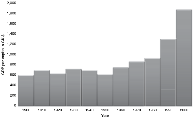
Figure 1.8 Reversal of fortune: Indian per capita GDP (1900–2000) (1990 International Geary-Khamis dollars)
1.8 Conclusion
In this chapter I have covered four centuries of Indian economic performance and living standards. Using data on real wages and GDP per capita, I have shown that the Great Divergence began before colonization. In 1600, the living standard in India was lower than that in Britain, but the difference was small. The gap widened during the seventeenth and eighteenth centuries as real wages and GDP per capita declined in India and rose in Britain. By the early nineteenth century, Indian real wages and GDP per capita stabilized at a low level. There were short periods of growth in the late nineteenth century, but Indian income stagnated during most of the colonial period, particularly in the first half of the twentieth century. Colonial policies of one of the richest countries in the world did not put India on the path of modern economic growth.
The Indian economy moved out of stagnation into growth after independence and 1950 was a turning point in India’s long-run economic growth. Another turning point came around 1980 with the adoption of a more liberal economic environment. Although Indian growth was low compared to East Asian economies, it was similar to most other countries in the developing world. The policies of regulation and state-directed industrialization under Nehru brought about a reversal of fortune in a decolonizing economy. The efficiency cost of an import-substituting industrialization policy was in part compensated by a rapid increase in capital accumulation.


