


1 Introduction
We let
 $\mathcal {C}$
denote the smooth concordance group of knots in
$\mathcal {C}$
denote the smooth concordance group of knots in
 $S^3$
. There are two fundamental measures of relationship between elements in
$S^3$
. There are two fundamental measures of relationship between elements in
 $\mathcal {C}$
: one is algebraic, linear independence; the other is geometric, the cobordism distance, a metric defined by
$\mathcal {C}$
: one is algebraic, linear independence; the other is geometric, the cobordism distance, a metric defined by
 $d(\mathcal {K}, \mathcal {J}) = g_4( \mathcal {K} \mathbin {\#} -\mathcal {J})$
, where
$d(\mathcal {K}, \mathcal {J}) = g_4( \mathcal {K} \mathbin {\#} -\mathcal {J})$
, where
 $g_4$
denotes the four-genus. Here, we combine these approaches to build a measure of how close knots are to being dependent in
$g_4$
denotes the four-genus. Here, we combine these approaches to build a measure of how close knots are to being dependent in
 $\mathcal {C}$
. Roughly stated, the distance between a pair of knots is defined as the minimum cobordism distance between all possible multiples and divisors of the knots. When made formal, this leads to the definition of the projective space of the concordance group
$\mathcal {C}$
. Roughly stated, the distance between a pair of knots is defined as the minimum cobordism distance between all possible multiples and divisors of the knots. When made formal, this leads to the definition of the projective space of the concordance group
 ${\mathbb P}(\mathcal {C})$
and a metric
${\mathbb P}(\mathcal {C})$
and a metric
 $\Delta $
built from the cobordism distance.
$\Delta $
built from the cobordism distance.
To make this more precise, recall that for a vector space V over a field
 ${\mathbb F}$
, there is relation on
${\mathbb F}$
, there is relation on
 $V^o = V \setminus 0$
defined by
$V^o = V \setminus 0$
defined by
 $v \sim w$
if there exists an
$v \sim w$
if there exists an
 $\alpha \in {\mathbb F}$
, such that
$\alpha \in {\mathbb F}$
, such that
 $w = \alpha v$
. To generalize this from vector spaces to abelian groups, we modify the relation so that it continues to be symmetric. For an abelian group G, we define a relation on the set
$w = \alpha v$
. To generalize this from vector spaces to abelian groups, we modify the relation so that it continues to be symmetric. For an abelian group G, we define a relation on the set
 $G^o = G \setminus 0$
as follows:
$G^o = G \setminus 0$
as follows:
 $a \sim b$
if there exist
$a \sim b$
if there exist
 $\alpha $
and
$\alpha $
and
 $\beta \in {\mathbb Z}$
and an element
$\beta \in {\mathbb Z}$
and an element
 $c \in G$
such that
$c \in G$
such that
 $a = \alpha c$
and
$a = \alpha c$
and
 $b = \beta c$
. This relation generates an equivalence relation on
$b = \beta c$
. This relation generates an equivalence relation on
 $G^0$
, and we denote the set of equivalence classes by
$G^0$
, and we denote the set of equivalence classes by
 ${\mathbb P}(G)$
, calling it the projective space of G. Symmetry could also be achieved using the condition that a and b have a common multiple, but this would have the effect of identifying all elements of finite order. Section 4 provides more details.
${\mathbb P}(G)$
, calling it the projective space of G. Symmetry could also be achieved using the condition that a and b have a common multiple, but this would have the effect of identifying all elements of finite order. Section 4 provides more details.
In the case of
 ${\mathbb P}(\mathcal {C})$
, we can define a metric based on the cobordism distance: again roughly stated, for classes
${\mathbb P}(\mathcal {C})$
, we can define a metric based on the cobordism distance: again roughly stated, for classes
 $[\mathcal {K}] \in {\mathbb P}(\mathcal {C})$
and
$[\mathcal {K}] \in {\mathbb P}(\mathcal {C})$
and
 $[\mathcal {J}] \in {\mathbb P}(\mathcal {C})$
, the distance
$[\mathcal {J}] \in {\mathbb P}(\mathcal {C})$
, the distance
 $\Delta ([\mathcal {K}], [\mathcal {J}])$
is defined by minimizing
$\Delta ([\mathcal {K}], [\mathcal {J}])$
is defined by minimizing
 $d(\mathcal {K}' , \mathcal {J}')$
over all representatives of the classes
$d(\mathcal {K}' , \mathcal {J}')$
over all representatives of the classes
 $[\mathcal {K}]$
and
$[\mathcal {K}]$
and
 $[\mathcal {J}]$
. To define this formally, there are some technical modifications required to ensure that the triangle inequality holds. Our goals include the following.
$[\mathcal {J}]$
. To define this formally, there are some technical modifications required to ensure that the triangle inequality holds. Our goals include the following.
-
• Define
 ${\mathbb P}(\mathcal {C})$
and study its basic properties. Letting
$\mathcal {T} \subset \mathcal {C}$
denote the torsion subgroup, we show that there is a natural bijection between
${\mathbb P}(\mathcal {C})$
and the disjoint union
${\mathbb P}(\mathcal {T}) \sqcup {\mathbb P}( \mathcal {C} / \mathcal {T})$
. We show that
${\mathbb P}(\mathcal {T})$
is either trivial or in bijective correspondence with
${\mathbb Z}_2^\infty \setminus 0$
depending on whether or not
$\mathcal {C}$
contains odd torsion. There is a natural bijection between
${\mathbb P}(\mathcal {C} /\mathcal {T})$
and the infinite rational projective space
${\mathbb Q}{\mathbb P}^\infty $
.
${\mathbb P}(\mathcal {C})$
and study its basic properties. Letting
$\mathcal {T} \subset \mathcal {C}$
denote the torsion subgroup, we show that there is a natural bijection between
${\mathbb P}(\mathcal {C})$
and the disjoint union
${\mathbb P}(\mathcal {T}) \sqcup {\mathbb P}( \mathcal {C} / \mathcal {T})$
. We show that
${\mathbb P}(\mathcal {T})$
is either trivial or in bijective correspondence with
${\mathbb Z}_2^\infty \setminus 0$
depending on whether or not
$\mathcal {C}$
contains odd torsion. There is a natural bijection between
${\mathbb P}(\mathcal {C} /\mathcal {T})$
and the infinite rational projective space
${\mathbb Q}{\mathbb P}^\infty $
. -
• Define the metric
$\Delta \colon \thinspace {\mathbb P}(\mathcal {C}) \times {\mathbb P}(\mathcal {C}) \to {\mathbb Z}$
. This gives
${\mathbb P}(\mathcal {C})$
the structure of a graph: vertices correspond to elements of the set, and two vertices are joined by an edge if they are at distance one. -
• Provide basic examples by studying the image of the set of
$(2,2k +1)$
-torus knots in
${\mathbb P}(\mathcal {C})$
. -
• Define the associated Vietoris–Rips simplicial complex
$\big | ({\mathbb P}(\mathcal {C}), \Delta )\big |$
and use twist knots to prove it is infinite-dimensional. -
• Identify basic problems related to
$({\mathbb P}(\mathcal {C}), \Delta )$
.


Background. We will work in the smooth category, but our work carries over to the topological locally flat category. In the 1960s, the combined work of Fox–Milnor [Reference Fox and Milnor8], Murasugi [Reference Murasugi19], Milnor [Reference Milnor18], Levine [Reference Levine15], and Tristam [Reference Tristram23] demonstrated that as an abstract group,
 $\mathcal {C} \cong {\mathbb Z}^\infty \oplus {\mathbb Z}_2^\infty \oplus G$
for some countable abelian group G. Nothing more is known today.
$\mathcal {C} \cong {\mathbb Z}^\infty \oplus {\mathbb Z}_2^\infty \oplus G$
for some countable abelian group G. Nothing more is known today.
Despite that lack of progress in understanding
 $\mathcal {C}$
from a purely algebraic standpoint, from a topological perspective, tremendous strides have been made. For instance, there are natural homomorphisms of
$\mathcal {C}$
from a purely algebraic standpoint, from a topological perspective, tremendous strides have been made. For instance, there are natural homomorphisms of
 $\mathcal {C}$
onto the topological concordance group and onto the higher dimension knot concordance groups. The kernels of these maps are now known to contain infinite free summands and to contain infinite 2-torsion; a few references include [Reference Endo4, Reference Jiang14, Reference Livingston17]. The primary examples used in proving the basic results about
$\mathcal {C}$
onto the topological concordance group and onto the higher dimension knot concordance groups. The kernels of these maps are now known to contain infinite free summands and to contain infinite 2-torsion; a few references include [Reference Endo4, Reference Jiang14, Reference Livingston17]. The primary examples used in proving the basic results about
 $\mathcal {C}$
have been built from two-bridge knots and
$\mathcal {C}$
have been built from two-bridge knots and
 $(2,2k+1)$
-torus knots. Continuing research concerns further understanding of the image of classes of knots, such as two-bridge knots, torus knots, and alternating knots, in
$(2,2k+1)$
-torus knots. Continuing research concerns further understanding of the image of classes of knots, such as two-bridge knots, torus knots, and alternating knots, in
 $\mathcal {C}$
. A few references include [Reference Feller and Park6, Reference Friedl, Livingston and Zentner9, Reference Lisca16].
$\mathcal {C}$
. A few references include [Reference Feller and Park6, Reference Friedl, Livingston and Zentner9, Reference Lisca16].
From a geometric perspective, understanding the four-genus of knots,
 $g_4(K)$
, was one of the early motivations for developing the concordance group, and the induced function
$g_4(K)$
, was one of the early motivations for developing the concordance group, and the induced function
 $g_4\colon \thinspace \mathcal {C} \to {\mathbb Z}$
continues to be studied. One highlight of this has been the study of differences of torus knots,
$g_4\colon \thinspace \mathcal {C} \to {\mathbb Z}$
continues to be studied. One highlight of this has been the study of differences of torus knots,
 $g_4(T_{p,q} \mathbin {\#} -T_{p',q'})$
(see, for instance, [Reference Baader2, Reference Feller and Park6, Reference Feller and Park7]).
$g_4(T_{p,q} \mathbin {\#} -T_{p',q'})$
(see, for instance, [Reference Baader2, Reference Feller and Park6, Reference Feller and Park7]).
1.1 Examples
A few examples will clarify the issues underlying the project here. We let
 $T_{2,2k+1}$
denote the
$T_{2,2k+1}$
denote the
 $(2,2k+1)$
-torus knot and let
$(2,2k+1)$
-torus knot and let
 $\mathcal {T}_{2,2k+1}$
denote its concordance class.
$\mathcal {T}_{2,2k+1}$
denote its concordance class.
-
• The classes
$\mathcal {T}_{2,5}$
and
$ \mathcal {T}_{2,11}$
are, in a sense, close to linear-dependent, since
$d(2\mathcal {T}_{2,5}, \mathcal {T}_{2,11}) =1$
. On the other hand,
$\mathcal {T}_{2,7}$
and
$ \mathcal {T}_{2,11}$
are further from being dependent:
$d(a \mathcal {T}_{2,7}, b \mathcal {T}_{2,11}) \ge 2$
, for all nonzero a and b. These are simple consequences of the results of Sections 2 and 3. -
• Issues related to the triangle inequality are illustrated by the following. For all a and b nonzero, the minimum of
$d(a \mathcal {T}_{2,41}, b \mathcal {T}_{2,61}) $
is
$2$
, realized by
$d( 3\mathcal {T}_{2,41} , 2\mathcal {T}_{2,61}) = 2$
; the minimum of
$d(a \mathcal {T}_{2,61}, b \mathcal {T}_{2,91}) $
is
$2$
, realized by
$d( 3\mathcal {T}_{2,61} , 2\mathcal {T}_{2,91}) = 2$
; and the minimum of
$d(a \mathcal {T}_{2,41}, b \mathcal {T}_{2,91}) $
is
$5$
, realized by
$d( 2\mathcal {T}_{2,41}, \mathcal {T}_{2,91}) = 5$
. This is discussed in Section 7.1. -
• The failure of transitivity that appears in defining
${\mathbb P}(G)$
is illustrated with the cyclic group
${\mathbb Z}_6$
. The pair of elements
$\{1, 2\}$
have a nonzero common multiple, as does the pair
$1$
and
$3$
. Yet the pair
$\{2,3\}$
does not have a common nonzero multiple. In the context of
$\mathcal {C}$
, we have
$2\mathcal {T}_{2,3}$
is in an infinite number of distinct cyclic subgroups, generated by elements of the form
$\mathcal {T}_{2,3} \mathbin {\#} \mathcal {J}$
for arbitrary 2-torsion elements
$\mathcal {J}$
. Thus, for instance, determining
$\Delta (\mathcal {T}_{p,q}, \mathcal {T}_{p',q'})$
entails determining the minimum of
$g_4( aT_{p,q} \mathbin {\#} bT_{p',q'} \mathbin {\#} J)$
for all nonzero a and b and for all knots J of finite order in
$\mathcal {C}$
.


1.2 Notation
It will be important to distinguish between a knot and the concordance class represented by the knot. To do so, we will change typeface; for instance, for the knot
 $K \subset S^3$
, we will write
$K \subset S^3$
, we will write
 $\mathcal {K} \subset \mathcal {C}$
for the concordance class represented by K. Later, when we place an equivalence relation on
$\mathcal {K} \subset \mathcal {C}$
for the concordance class represented by K. Later, when we place an equivalence relation on
 $\mathcal {C}$
to form the projective space,
$\mathcal {C}$
to form the projective space,
 ${\mathbb P}(\mathcal {C})$
, the equivalence class of
${\mathbb P}(\mathcal {C})$
, the equivalence class of
 $\mathcal {K} \in \mathcal {C}$
will be denoted
$\mathcal {K} \in \mathcal {C}$
will be denoted
 $[\mathcal {K}] \in {\mathbb P}(\mathcal {C})$
.
$[\mathcal {K}] \in {\mathbb P}(\mathcal {C})$
.
The functions
 $g_4$
can be defined on the set of knots or on
$g_4$
can be defined on the set of knots or on
 $\mathcal {C}$
. Similarly, we can refer to the distance
$\mathcal {C}$
. Similarly, we can refer to the distance
 $d(K,J)$
or
$d(K,J)$
or
 $d(\mathcal {K}, \mathcal {J})$
, working with knots or concordance classes. This ambiguity should not be problematic, so we do not add to the notation to distinguish these functions based on their domains.
$d(\mathcal {K}, \mathcal {J})$
, working with knots or concordance classes. This ambiguity should not be problematic, so we do not add to the notation to distinguish these functions based on their domains.
1.3 Outline
Sections 2 and 3 discuss a basic family of examples, that of two-stranded torus knots,
 $T_{2,2k+1}$
. In this setting, we explore the problem of minimizing
$T_{2,2k+1}$
. In this setting, we explore the problem of minimizing
 $d(aT_{2,2k+1}, bT_{2,2n+1})$
over all
$d(aT_{2,2k+1}, bT_{2,2n+1})$
over all
 $a\ne 0$
and
$a\ne 0$
and
 $ b \ne 0$
. The first of these two sections concerns geometric tools that provide upper bounds; the next section uses signature functions to find lower bounds. We will define
$ b \ne 0$
. The first of these two sections concerns geometric tools that provide upper bounds; the next section uses signature functions to find lower bounds. We will define
 $\overline {d}(K, J) = \min \{ d(aK, bJ )\ \big | \ a, b \ne 0\}$
. Elementary consequences of the work in these sections are the following results presented in Section 3.6:
$\overline {d}(K, J) = \min \{ d(aK, bJ )\ \big | \ a, b \ne 0\}$
. Elementary consequences of the work in these sections are the following results presented in Section 3.6:
-
•
$\overline {d} (\mathcal {T}_{2,2k+1}, \mathcal {T}_{2,2n+1})$
goes to infinity for fixed k as n grows. The growth rate is of order
$ {n}/{2k}$
. -
• For fixed
$N>0$
, the set of values
$\overline {d}(\mathcal {T}_{2,2k+1}, \mathcal {T}_{2,2n+1})$
for all k and n satisfying
${\big | n - k \big | \le N}$
is bounded. -
• The function
$\overline {d} \colon \thinspace \mathcal {C} \times \mathcal {C} \to {\mathbb Z}$
does not satisfy the triangle inequality.


In Section 4, we develop the formal algebra that permits us to define the appropriate equivalence relation and form the quotient space
 ${\mathbb P}(\mathcal {C})$
. In our setting, we could restrict our algebraic discussion to general abelian groups, but the natural map
${\mathbb P}(\mathcal {C})$
. In our setting, we could restrict our algebraic discussion to general abelian groups, but the natural map
 ${\mathcal {C} \to \mathcal {C} \otimes {\mathbb Q}}$
leads us to consider projectivizing modules over
${\mathcal {C} \to \mathcal {C} \otimes {\mathbb Q}}$
leads us to consider projectivizing modules over
 ${\mathbb Q}$
, and ultimately modules M over arbitrary integral domains. In Section 5, we define a canonical metric on
${\mathbb Q}$
, and ultimately modules M over arbitrary integral domains. In Section 5, we define a canonical metric on
 ${\mathbb P}(M)$
for a given integer-valued metric on M, and Section 6 considers basic properties of that metric in the case of
${\mathbb P}(M)$
for a given integer-valued metric on M, and Section 6 considers basic properties of that metric in the case of
 ${\mathbb P}(\mathcal {C})$
.
${\mathbb P}(\mathcal {C})$
.
In Section 7, we discuss tools for computing a pseudometric
 $\delta $
that is initially defined on
$\delta $
that is initially defined on
 ${\mathbb P}(\mathcal {C})$
. This discussion is based on the signature function, as developed in Section 3.
${\mathbb P}(\mathcal {C})$
. This discussion is based on the signature function, as developed in Section 3.
Section 8 concerns the metric
 $\Delta \colon \thinspace {\mathbb P}(\mathcal {C}) \times {\mathbb P}(\mathcal {C}) \to {\mathbb Z}$
. Computations are much more difficult, so we restrict ourselves to the setting of
$\Delta \colon \thinspace {\mathbb P}(\mathcal {C}) \times {\mathbb P}(\mathcal {C}) \to {\mathbb Z}$
. Computations are much more difficult, so we restrict ourselves to the setting of
 $(2,2k\! +\!1)$
-torus knots and the analysis of small balls in the subset of
$(2,2k\! +\!1)$
-torus knots and the analysis of small balls in the subset of
 ${\mathbb P}(\mathcal {C})$
consisting of elements represented by these knots. It is worth mentioning now that for any class
${\mathbb P}(\mathcal {C})$
consisting of elements represented by these knots. It is worth mentioning now that for any class
 $\mathcal {K} $
in the span of such torus knots, there are concordance class
$\mathcal {K} $
in the span of such torus knots, there are concordance class
 $\mathcal {J} \in \mathcal {C}$
satisfying
$\mathcal {J} \in \mathcal {C}$
satisfying
 $ \mathcal {J} \in [\mathcal {K}]$
, but for which
$ \mathcal {J} \in [\mathcal {K}]$
, but for which
 $\mathcal {J}$
is not represented by a knot in the span of torus knots. Here is a simple example. Let
$\mathcal {J}$
is not represented by a knot in the span of torus knots. Here is a simple example. Let
 $\mathcal {J} $
be any element of order two in
$\mathcal {J} $
be any element of order two in
 $\mathcal {C}$
. Then
$\mathcal {C}$
. Then
 $2(\mathcal {T}_{2,3} \mathbin {\#} \mathcal {J}) = 2\mathcal {T}_{2,3}$
, so both represent the same element in
$2(\mathcal {T}_{2,3} \mathbin {\#} \mathcal {J}) = 2\mathcal {T}_{2,3}$
, so both represent the same element in
 ${\mathbb P}(\mathcal {C})$
; however,
${\mathbb P}(\mathcal {C})$
; however,
 $\mathcal {T}_{2,3} \mathbin {\#} J$
is not in the span of torus knots.
$\mathcal {T}_{2,3} \mathbin {\#} J$
is not in the span of torus knots.
A challenging problem asks, for each subgroup
 $\mathcal {S} \subset \mathcal {C}$
, whether the inclusion
$\mathcal {S} \subset \mathcal {C}$
, whether the inclusion
 ${\mathbb P}(\mathcal {S}) \to {\mathbb P}(\mathcal {C})$
is an isometry. This and other problems are summarized in Section 11.
${\mathbb P}(\mathcal {S}) \to {\mathbb P}(\mathcal {C})$
is an isometry. This and other problems are summarized in Section 11.
2 Torus knots,
$T_{2,2k+1}$
: geometric constructions

The space
 ${\mathbb P}(\mathcal {C})$
will provide a structure for exploring knot concordance, but ultimately the questions that arise can only be understood by constructing surfaces in
${\mathbb P}(\mathcal {C})$
will provide a structure for exploring knot concordance, but ultimately the questions that arise can only be understood by constructing surfaces in
 $B^4$
bounded by connected sums of the form
$B^4$
bounded by connected sums of the form
 $aK \mathbin {\#} -bJ$
and then finding lower bounds on the genus of such surfaces. In this section, we consider the construction of surfaces bounded by linear combinations of pairs
$aK \mathbin {\#} -bJ$
and then finding lower bounds on the genus of such surfaces. In this section, we consider the construction of surfaces bounded by linear combinations of pairs
 $\{T_{2,2k+1}, T_{2,2n+1}\}$
and then focus on the special case of minimizing
$\{T_{2,2k+1}, T_{2,2n+1}\}$
and then focus on the special case of minimizing
 $g_4(T_{2,2k+1} \mathbin {\#} - \beta T_{2,2n+1})$
. In the next section, we use the signature function to show that minimizing
$g_4(T_{2,2k+1} \mathbin {\#} - \beta T_{2,2n+1})$
. In the next section, we use the signature function to show that minimizing
 $g_4(a T_{2,2k+1} \mathbin {\#} - b T_{2,2n+1})$
over all a and b can be reduced to a finite set of such pairs, and we completely resolve the problem of minimizing
$g_4(a T_{2,2k+1} \mathbin {\#} - b T_{2,2n+1})$
over all a and b can be reduced to a finite set of such pairs, and we completely resolve the problem of minimizing
 $g_4( T_{2,2k+1} \mathbin {\#} - b T_{2,2n+1})$
. We also provide examples for which the overall minimum over all a and b is not achieved with
$g_4( T_{2,2k+1} \mathbin {\#} - b T_{2,2n+1})$
. We also provide examples for which the overall minimum over all a and b is not achieved with
 $a =1$
.
$a =1$
.
At this point, we note an interesting aspect of the family of
 $(2,2k+1)$
-torus knots: from the perspective of Heegaard Floer theory, they all appear to be linearly dependent: there is a chain homotopy equivalence
$(2,2k+1)$
-torus knots: from the perspective of Heegaard Floer theory, they all appear to be linearly dependent: there is a chain homotopy equivalence
 $\operatorname {{\mathrm {CFK}}}^\infty (nT_{2,2k+1}) \oplus A_1 \simeq \operatorname {{\mathrm {CFK}}}^\infty (kT_{2,2n+1}) \oplus A_2$
for some pair of acyclic complexes
$\operatorname {{\mathrm {CFK}}}^\infty (nT_{2,2k+1}) \oplus A_1 \simeq \operatorname {{\mathrm {CFK}}}^\infty (kT_{2,2n+1}) \oplus A_2$
for some pair of acyclic complexes
 $A_1$
and
$A_1$
and
 $A_2$
. More generally, Feller and Krcatovich [Reference Feller and Krcatovich5] have demonstrated the limited ability of Heegaard Floer Upsilon to obstruct linear dependance in
$A_2$
. More generally, Feller and Krcatovich [Reference Feller and Krcatovich5] have demonstrated the limited ability of Heegaard Floer Upsilon to obstruct linear dependance in
 $\mathcal {C}$
among general torus knots. If one moves to the realm of involutive Heegaard Floer theory, some limited results concerning torus knots
$\mathcal {C}$
among general torus knots. If one moves to the realm of involutive Heegaard Floer theory, some limited results concerning torus knots
 $T_{2,2k+1}$
become available (see [Reference Hendricks and Manolescu12]).
$T_{2,2k+1}$
become available (see [Reference Hendricks and Manolescu12]).
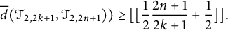
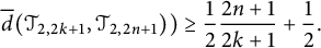
2.1 Basic construction
A Seifert surface for
 $T_{2,2k+1}$
is constructed by attaching
$T_{2,2k+1}$
is constructed by attaching
 $2k$
once twisted bands to a disk. Figures 1 and 2 are schematic representations of Seifert surfaces for
$2k$
once twisted bands to a disk. Figures 1 and 2 are schematic representations of Seifert surfaces for
 $T_{2, 13} \mathbin {\#} -2T_{2,5}$
and
$T_{2, 13} \mathbin {\#} -2T_{2,5}$
and
 $T_{2, 13} \mathbin {\#} -3T_{2,5}$
. Curves drawn on the surface represent unlinks with 0 framing on the surfaces. (In the first illustration, there are eight such curves; each one goes over a band on the top and a band on the bottom. In the second illustration, there are 10 such curves.) Surgery can be performed on the surfaces in
$T_{2, 13} \mathbin {\#} -3T_{2,5}$
. Curves drawn on the surface represent unlinks with 0 framing on the surfaces. (In the first illustration, there are eight such curves; each one goes over a band on the top and a band on the bottom. In the second illustration, there are 10 such curves.) Surgery can be performed on the surfaces in
 $B^4$
to yield surfaces of lower genus than the Seifert surfaces, thus giving upper bounds on the four-genus of the knots.
$B^4$
to yield surfaces of lower genus than the Seifert surfaces, thus giving upper bounds on the four-genus of the knots.
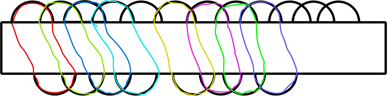
Figure 1: A schematic of a Seifert surface for
 $T_{2,13} - 2T_{2,5}$
and surgery curves.
$T_{2,13} - 2T_{2,5}$
and surgery curves.
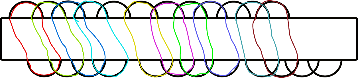
Figure 2: A schematic of a Seifert surface for
 $T_{2,13} - 3T_{2,5}$
and surgery curves.
$T_{2,13} - 3T_{2,5}$
and surgery curves.
2.2 Application to
$T_{2,2n+1} -aT_{2,2k+1}$

Figures 1 and 2 illustrate two possibilities for connected sums
 $T_{2,2n+1} \mathbin {\#} - aT_{2,2k+1}$
, where
$T_{2,2n+1} \mathbin {\#} - aT_{2,2k+1}$
, where
 $n>k$
. In each case, there is an elementary computation of the genus of the resulting surface in
$n>k$
. In each case, there is an elementary computation of the genus of the resulting surface in
 $B^4$
. With a bit of experimenting, one might suspect that the minimum four-genus of
$B^4$
. With a bit of experimenting, one might suspect that the minimum four-genus of
 $T_{2,2n+1} \mathbin {\#} - aT_{2, 2k+1}$
is achieved when a is close to
$T_{2,2n+1} \mathbin {\#} - aT_{2, 2k+1}$
is achieved when a is close to
 $\alpha = \lfloor \frac {2n+1}{2k+1}\rfloor $
. Here, we present the computation for the two values of a closest to
$\alpha = \lfloor \frac {2n+1}{2k+1}\rfloor $
. Here, we present the computation for the two values of a closest to
 $\alpha $
. Once we consider signatures, we will prove that one of these surfaces realizes the minimum. As mentioned earlier, it is not always the case the
$\alpha $
. Once we consider signatures, we will prove that one of these surfaces realizes the minimum. As mentioned earlier, it is not always the case the
 $\min \{ d(aT_{2,2k+1}, bT_{2, 2n+1})\ \big | \ a, b \ne 0\}$
is realized with
$\min \{ d(aT_{2,2k+1}, bT_{2, 2n+1})\ \big | \ a, b \ne 0\}$
is realized with
 $b= 1$
.
$b= 1$
.
Theorem 2.1 For
 $0 < k <n$
, let
$0 < k <n$
, let
 $\alpha = \lfloor \frac {2n+1}{2k+1}\rfloor $
.
$\alpha = \lfloor \frac {2n+1}{2k+1}\rfloor $
.
-
(1)
$ g_4(T_{2,2n+1} \mathbin {\#} - \alpha T_{2, 2k+1} ) \le n - \alpha k.$
-
(2) If
$2k+1$
does not divide
$2n+1$
, then
$ g_4(T_{2,2n+1} \mathbin {\#} - (\alpha +1) T_{2, 2k+1} ) \le \alpha (k+1) +k- n .$


Proof The genus of the surface before the surgery is one half the total number of bands. Surgery reduces the genus by the number of surgery curves, which is one half the number of bands that have surgery curves going over them. We call the bands that do not have surgery curves going over them free bands. Thus, the genus after surgery is one half the number of free bands. For instance, in Figure 1, there are four such bands, all on top. In Figure 2, there are also four such bands, two on top and two on the bottom.
In the first case, all the free bands are on top. There are two types: those resulting from gaps and those at the end. The count is
 $(\alpha -1) + (2n - \big (\alpha (2 k+1) -1)\big )$
In the second case, there are
 $\alpha $
free bands on the top (this uses the fact that
$\alpha $
free bands on the top (this uses the fact that
 $2k+1$
does not divide
$2k+1$
does not divide
 $2n +1$
). On the bottom, there are
$2n +1$
). On the bottom, there are
 $2k - \big ( 2n - \alpha (2k+1) \big ) $
free bands. The result now follows from an algebraic simplification.
$2k - \big ( 2n - \alpha (2k+1) \big ) $
free bands. The result now follows from an algebraic simplification.
3 Torus knots,
$T_{2,2k+1}$
: signature results

The signature function provides strong bounds on the four-genus of knots. In this section, we will consider the special case of torus knots of the form
 $T_{2,2k+1}$
and undertake signature function calculations related to determining the distance between a pair
$T_{2,2k+1}$
and undertake signature function calculations related to determining the distance between a pair
 $aT_{2,2k+1}$
and
$aT_{2,2k+1}$
and
 $bT_{2,2n+1}$
.
$bT_{2,2n+1}$
.
In the rest of this section, we will restrict our attention to the case that the parameters a and b are positive. This is motivated by two observations. First, if a and b are of opposite sign, then the classical Murasugi signature [Reference Murasugi19] determines that the four-genus satisfies
 $g_4(aT_{2,2k+1} \mathbin {\#} -bT_{2,2n+1}) = \big | ak - bn\big |$
. Second, if one considers more general pairs of positive torus knots, still with opposite signs, then the signature function is not sufficient to determine the four-genus
$g_4(aT_{2,2k+1} \mathbin {\#} -bT_{2,2n+1}) = \big | ak - bn\big |$
. Second, if one considers more general pairs of positive torus knots, still with opposite signs, then the signature function is not sufficient to determine the four-genus
 $g_4(aT_{p,q} \mathbin {\#} -bT_{p',q'})$
, but the Ozsváth–Szabó
$g_4(aT_{p,q} \mathbin {\#} -bT_{p',q'})$
, but the Ozsváth–Szabó
 $\tau $
–invariant [Reference Ozsváth and Szabó20] and the Rasmussen s-invariant [Reference Rasmussen21] do suffice. On the other hand, it is remarkable how challenging it is to analyze the case in which the signs are the same, and perhaps surprising that signature functions can be effective while more modern methods yield little information.
$\tau $
–invariant [Reference Ozsváth and Szabó20] and the Rasmussen s-invariant [Reference Rasmussen21] do suffice. On the other hand, it is remarkable how challenging it is to analyze the case in which the signs are the same, and perhaps surprising that signature functions can be effective while more modern methods yield little information.
3.1 Signature functions
In order to simplify our calculations, rather than work with the (two-sided averaged) Levine–Tristram signature function,
 $\sigma _K(\omega )$
, we will normalize and define
$\sigma _K(\omega )$
, we will normalize and define
 $\sigma ^{\prime }_K(\omega ) =-\sigma _K(\omega ) /2 $
. To further simplify notation, instead of working with unit complex numbers on the upper half-circle,
$\sigma ^{\prime }_K(\omega ) =-\sigma _K(\omega ) /2 $
. To further simplify notation, instead of working with unit complex numbers on the upper half-circle,
 $\omega $
, we will change variables so that domain is
$\omega $
, we will change variables so that domain is
 $[0,1]$
by setting
$[0,1]$
by setting
 $\omega = e^{ \pi i t }$
. The next well-known result follows from the work of Tristram [Reference Tristram23] and Viro [Reference Viro24].
$\omega = e^{ \pi i t }$
. The next well-known result follows from the work of Tristram [Reference Tristram23] and Viro [Reference Viro24].
Proposition 3.1 For all knots K and for all
 $t \in [0,1]$
,
$t \in [0,1]$
,
 $g_4(K) \ge \big | \sigma ^{\prime }_K(t)\big |.$
In light of this, we define the function that maximizes this bound.
Definition 3.1 For a knot K,
 $S(K) = \max _{0 \le t \le 1}\{\big | \sigma ^{\prime }_K(t) \big | \}$
.
$S(K) = \max _{0 \le t \le 1}\{\big | \sigma ^{\prime }_K(t) \big | \}$
.
3.2 Signature functions of
$T_{2,2k+1}$
.

A standard result for
 $2$
-stranded torus knot is the following.
$2$
-stranded torus knot is the following.
Proposition 3.2 If
 $1 \le j \le k$
and
$1 \le j \le k$
and
 $ \frac {2j-1}{2k+1} < t < \frac {2j+1}{2k+1}$
, then
$ \frac {2j-1}{2k+1} < t < \frac {2j+1}{2k+1}$
, then
 $\sigma ^{\prime }_{T_{2,2k+1}}(t) = j$
. If
$\sigma ^{\prime }_{T_{2,2k+1}}(t) = j$
. If
 $t < \frac {1}{2k +1}$
, then
$t < \frac {1}{2k +1}$
, then
 $\sigma ^{\prime }_{T_{2,2k+1}}(t) = 0$
.
$\sigma ^{\prime }_{T_{2,2k+1}}(t) = 0$
.
It is clear from Theorem 2.1 that in studying the difference
 $ bT_{2, 2n+1} \mathbin {\#} -aT_{2,2k+1}$
, care is required in the special case that
$ bT_{2, 2n+1} \mathbin {\#} -aT_{2,2k+1}$
, care is required in the special case that
 $\frac {2n+1}{2k+1}$
is an integer. Because of this, the floor function arises naturally in the calculations, but it has to be slightly modified.
$\frac {2n+1}{2k+1}$
is an integer. Because of this, the floor function arises naturally in the calculations, but it has to be slightly modified.
Definition 3.2 We will write
 $\lfloor \lfloor x \rfloor \rfloor $
for the function that equals
$\lfloor \lfloor x \rfloor \rfloor $
for the function that equals
 $ \lfloor x \rfloor $
if x is not an integer and
$ \lfloor x \rfloor $
if x is not an integer and
 $ \lfloor x \rfloor - 1$
if
$ \lfloor x \rfloor - 1$
if
 $x \in {\mathbb Z}$
. More concisely,
$x \in {\mathbb Z}$
. More concisely,
 $\lfloor \lfloor x \rfloor \rfloor = \lceil x \rceil -1$
.
$\lfloor \lfloor x \rfloor \rfloor = \lceil x \rceil -1$
.
A simple calculation now yields the following result.
Corollary 3.3 Let
 $K =bT_{2,2n+1} \mathbin {\#} - aT_{2,2k+1}$
with
$K =bT_{2,2n+1} \mathbin {\#} - aT_{2,2k+1}$
with
 $0< k<n$
and
$0< k<n$
and
 $a, b>0$
. For sufficiently small
$a, b>0$
. For sufficiently small
 $\epsilon $
with
$\epsilon $
with
 $\epsilon>0$
, we have:
$\epsilon>0$
, we have:
-
(1)
$\sigma ^{\prime }_K(\frac {1}{2k+1} - \epsilon ) = b \lfloor \lfloor \frac {1}{2}\frac {2n+1}{2k+1} +\frac {1}{2} \rfloor \rfloor \ge b$
. -
(2)
$\sigma ^{\prime }_K(1) = bn -ak $
. -
(3)
$\sigma ^{\prime }_K(\frac {2k-1}{2k+1} + \epsilon ) =bn -ak -b \lfloor \lfloor \frac {2n+1}{2k+1} \rfloor \rfloor $
.


Corollary 3.4 If k and n satisfy
 $0 < k <n$
and
$0 < k <n$
and
 $N>0$
, then the set of positive pairs
$N>0$
, then the set of positive pairs
 $a $
and b such that
$a $
and b such that
 $S(bT_{2, 2n+1} \mathbin {\#} - aT_{2,2k+1}) \le N $
is finite.
$S(bT_{2, 2n+1} \mathbin {\#} - aT_{2,2k+1}) \le N $
is finite.
Proof Suppose that
 $S(bT_{2, 2n+1} \mathbin {\#} - aT_{2,2k+1}) \le N $
with
$S(bT_{2, 2n+1} \mathbin {\#} - aT_{2,2k+1}) \le N $
with
 $a>0$
and
$a>0$
and
 $b>0$
. Condition (1) of Corollary 3.3 implies that
$b>0$
. Condition (1) of Corollary 3.3 implies that
 $0< b \le N$
. For each value of b in that interval, Condition (2) implies that the set of possible values of a is also finite.
$0< b \le N$
. For each value of b in that interval, Condition (2) implies that the set of possible values of a is also finite.
3.3 The case of
$b=1$
: minimizing
$g_4(T_{2,2n+1} \mathbin {\#} - aT_{2, 2k+1})$


Theorem 3.5 Let
 $\alpha = \lfloor \frac {2n+1}{2k+1} \rfloor $
. The minimum value of
$\alpha = \lfloor \frac {2n+1}{2k+1} \rfloor $
. The minimum value of
 $g_4(T_{2,2n+1} - aT_{2, 2k+1})$
is achieved when
$g_4(T_{2,2n+1} - aT_{2, 2k+1})$
is achieved when
 $a = \alpha $
or
$a = \alpha $
or
 $\alpha +1$
, with the two possible values given by:
$\alpha +1$
, with the two possible values given by:
-
•
$g_4(T_{2,2n+1} \mathbin {\#} - \alpha T_{2, 2k+1})= n - \alpha k $
. -
•
$g_4(T_{2,2n+1} \mathbin {\#} - (\alpha +1) T_{2, 2k+1} )= (\alpha +1)(k+1) - n -1 $
.


Proof Let
 $F(a)$
denote the signature function bound on
$F(a)$
denote the signature function bound on
 $g_4(T_{2,2n+1} \mathbin {\#} - a T_{2, 2k+1})$
. We consider two cases:
$g_4(T_{2,2n+1} \mathbin {\#} - a T_{2, 2k+1})$
. We consider two cases:
 $a \le \alpha $
and
$a \le \alpha $
and
 $a \ge \alpha +1$
.
$a \ge \alpha +1$
.
Case 1:
 $a \le \alpha $
. In this case, we consider the signature at
$a \le \alpha $
. In this case, we consider the signature at
 $t = 1$
. Noting that
$t = 1$
. Noting that
 $n-ak \ge 0$
, we find that
$n-ak \ge 0$
, we find that
 $F(a) \ge n -ak$
. This bound is realized at
$F(a) \ge n -ak$
. This bound is realized at
 $a = \alpha $
, so we have
$a = \alpha $
, so we have
 $F(\alpha ) = n - \alpha k$
and
$F(\alpha ) = n - \alpha k$
and
 $F(a)> F(\alpha )$
for all
$F(a)> F(\alpha )$
for all
 $a < \alpha $
.
$a < \alpha $
.
Case 2:
 $a \ge \alpha +1$
. In this case, we consider the signature at
$a \ge \alpha +1$
. In this case, we consider the signature at
 $t = \frac {2k-1}{2k+1} + \epsilon $
for some small
$t = \frac {2k-1}{2k+1} + \epsilon $
for some small
 $\epsilon $
. In this case, we have
$\epsilon $
. In this case, we have
 $F(a) \ge ak - n + \lfloor \frac {2n+1}{2k+1} \rfloor $
. This bound is realized when
$F(a) \ge ak - n + \lfloor \frac {2n+1}{2k+1} \rfloor $
. This bound is realized when
 $a = \alpha +1$
.
$a = \alpha +1$
.
Now, we can combine these two cases. If
 $S(\alpha ) \le S(\alpha +1)$
, then
$S(\alpha ) \le S(\alpha +1)$
, then
 $S(\alpha ) \le S(a)$
for all a and
$S(\alpha ) \le S(a)$
for all a and
 $g_4(T_{2,2n+1} \mathbin {\#} - a T_{2, 2k+1})$
is minimized at
$g_4(T_{2,2n+1} \mathbin {\#} - a T_{2, 2k+1})$
is minimized at
 $a - \alpha $
. Similarly if
$a - \alpha $
. Similarly if
 $S(\alpha + 1) \le S(\alpha )$
.
$S(\alpha + 1) \le S(\alpha )$
.
3.4 Basic examples
We begin with a few examples. In each case, we assume either a or b is nonzero.
Example 3.6
 $ { \min \{ g_4(bT_{2,23} \mathbin {\#} - aT_{2,7}), a,b \in {\mathbb Z}_{>0} \} = g_4( T_{2,23} \mathbin {\#} - 3T_{2,7}) = 2.} $
In this case, we have
$ { \min \{ g_4(bT_{2,23} \mathbin {\#} - aT_{2,7}), a,b \in {\mathbb Z}_{>0} \} = g_4( T_{2,23} \mathbin {\#} - 3T_{2,7}) = 2.} $
In this case, we have
 $n=11$
and
$n=11$
and
 $k =3$
.
$k =3$
.
Applying Corollary 3.3, we find
 $$\begin{align*}g_4( bT_{2,23} - aT_{2,7}) \ge S(bT_{2,23} \mathbin{\#} - aT_{2,7}) \ge \max\{ 2b , \big| 11b - 3a\big|, \big| 8b - 3a \big|\}. \end{align*}$$
By Theorem 2.1, we have
 $g_4(T_{2,23} \mathbin {\#} - 3T_{2,7} )\le 2$
. We claim that
$g_4(T_{2,23} \mathbin {\#} - 3T_{2,7} )\le 2$
. We claim that
 $(a,b)= (3,1)$
is the unique positive pair for which
$(a,b)= (3,1)$
is the unique positive pair for which
 $\max \{ 2b , \big | 11b - 3a\big |, \big | 8b - 3a \big |\} \le 2$
. Clearly, if
$\max \{ 2b , \big | 11b - 3a\big |, \big | 8b - 3a \big |\} \le 2$
. Clearly, if
 $b = 0$
, then a must equal 0 for the inequality to hold, and if
$b = 0$
, then a must equal 0 for the inequality to hold, and if
 $b>1$
, then the inequality cannot hold. In the case that
$b>1$
, then the inequality cannot hold. In the case that
 $b = 1$
, one observes that for
$b = 1$
, one observes that for
 $\big |11-3a\big |$
and
$\big |11-3a\big |$
and
 $\big |8-3a\big |$
to both be less than 3, we must have
$\big |8-3a\big |$
to both be less than 3, we must have
 $a=3$
.
$a=3$
.
Example 3.7
 $ { \min \{g_4(bT_{2,17} \mathbin {\#} - aT_{2,11}), a, b \in {\mathbb Z}_{>0} \} = g_4( 2T_{2,17} \mathbin {\#} - 3T_{2,7}) = 2.} $
Here, we present a case in which
$ { \min \{g_4(bT_{2,17} \mathbin {\#} - aT_{2,11}), a, b \in {\mathbb Z}_{>0} \} = g_4( 2T_{2,17} \mathbin {\#} - 3T_{2,7}) = 2.} $
Here, we present a case in which
 $g_4(bT_{2,2n+1} \mathbin {\#} - aT_{2, 2k+1})$
is not realized by
$g_4(bT_{2,2n+1} \mathbin {\#} - aT_{2, 2k+1})$
is not realized by
 $g_4(T_{2,2n+1} \mathbin {\#} - a T_{2, 2k+1})$
for any a. Let
$g_4(T_{2,2n+1} \mathbin {\#} - a T_{2, 2k+1})$
for any a. Let
 $k=5$
and
$k=5$
and
 $n=8$
. By Corollary 3.3, if we consider combinations of the form
$n=8$
. By Corollary 3.3, if we consider combinations of the form
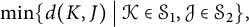
 $ T_{2,17} \mathbin {\#} - aT_{2,11}$
(Figure 3), we have
$ T_{2,17} \mathbin {\#} - aT_{2,11}$
(Figure 3), we have
 $$\begin{align*}S(T_{2,17} \mathbin{\#} - aT_{2,11}) \ge \max \{ 1, \big|8 - 5a\big|, \big|7 - 5a\big| \}. \end{align*}$$
For all values of a, this is always at least 3.

Figure 3:
 $\sigma _K(\omega )$
for
$\sigma _K(\omega )$
for
 $K =T_{2,17} \mathbin {\#} - 2T_{2,11}$
and
$K =T_{2,17} \mathbin {\#} - 2T_{2,11}$
and
 $K =2T_{2,17} \mathbin {\#} - 3T_{2,11}$
.
$K =2T_{2,17} \mathbin {\#} - 3T_{2,11}$
.
For general b, we have
 $$\begin{align*}S(bT_{2,17} \mathbin{\#} - aT_{2,11}) \ge \max \{ b, \big|8b - 5a\big|, \big|7b - 5a\big| \}. \end{align*}$$
For
 $b = 2$
and
$b = 2$
and
 $a = 3$
, the maximum is 2, and one can quickly check that this is the only pair for which the maximum of 2 is realized.
$a = 3$
, the maximum is 2, and one can quickly check that this is the only pair for which the maximum of 2 is realized.
We finally observe that
 $g_4(2 T_{2,17} \mathbin {\#} - 3T_{2,11}) = 2$
. If we draw a schematic for this difference, there are two groups of 16 bands on the top and 3 groups of 10 bands on the bottom. All 10 bands of the bottom-left group can be surgered, as can the 10 bands of the bottom-right group. This leaves five bands free on each of the top two groups. These can be combined with bands on the bottom-central group to perform surgery on nine more curves. Thus, we have reduced the genus by
$g_4(2 T_{2,17} \mathbin {\#} - 3T_{2,11}) = 2$
. If we draw a schematic for this difference, there are two groups of 16 bands on the top and 3 groups of 10 bands on the bottom. All 10 bands of the bottom-left group can be surgered, as can the 10 bands of the bottom-right group. This leaves five bands free on each of the top two groups. These can be combined with bands on the bottom-central group to perform surgery on nine more curves. Thus, we have reduced the genus by
 $10 + 10 +9 = 29$
. Finally,
$10 + 10 +9 = 29$
. Finally,
 $31-29 = 2$
, yielding the minimum.
$31-29 = 2$
, yielding the minimum.
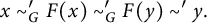
Figure 3 illustrates two of the signature functions that were implicitly considered above. (The t-axis is labeled from 0 to 1,000, indicating that the signature function was evaluated at points
 $i/1,000$
.)
$i/1,000$
.)
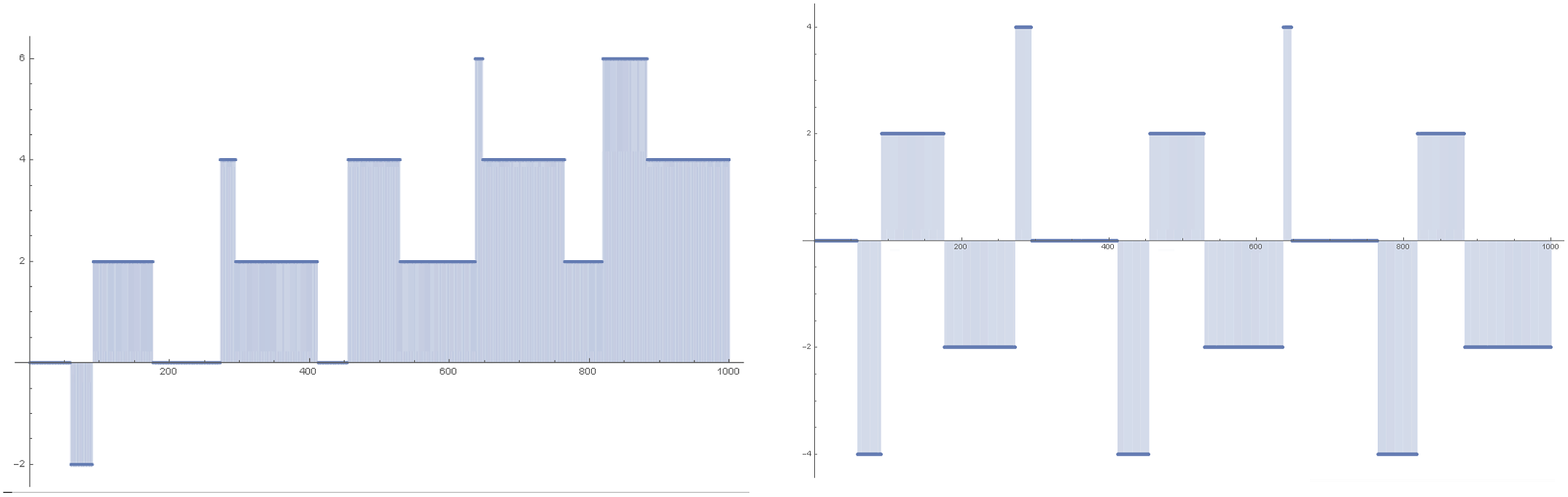
Figure 4:
 $\sigma _K(\omega )$
for
$\sigma _K(\omega )$
for
 $K =T_{2,17} \mathbin {\#} - 2T_{2,11}$
and
$K =T_{2,17} \mathbin {\#} - 2T_{2,11}$
and
 $K =2T_{2,17} \mathbin {\#} - 3T_{2,11}$
.
$K =2T_{2,17} \mathbin {\#} - 3T_{2,11}$
.
3.5 Failure of the triangle inequality
Our final example is the most technical. It will be used later to demonstrate the failure of the triangle inequality.
-
(1) Min
$\{ g_4( bT_{2,61} \mathbin {\#} - aT_{2,41})\} = 2$
, realized by
$g_4(2 T_{2,61}\mathbin {\#} - 3T_{2,41}) =2$
. -
(2) Min
$\{ g_4(bT_{2,91}\mathbin {\#} - aT_{2,61})\} = 2$
, realized by
$g_4(2T_{2,91} \mathbin {\#} - 3T_{2,61}) = 2$
. -
(3) Min
$\{ g_4(bT_{2,91}\mathbin {\#} - aT_{2,41})\} = 5$
, realized by
$g_4( T_{2,91} \mathbin {\#} - 2T_{2,41}) = 5$
.


We now work through each case.
-
(1) A construction similar to the one used to show
$g_4(2 T_{2,17} \mathbin {\#} - 3T_{2,11}) =2$
demonstrates that
$g_4(2 T_{2,61} \mathbin {\#} - 3T_{2,41}) \le 2$
. Thus, we need to show that 2 is the minimum. Here,
$n= 30$
and
$k=20$
. Applying Corollary 3.3, we find
$$\begin{align*}S(bT_{2,61} \mathbin{\#} - aT_{2,41}) \ge \max\{ b , \big| 30b - 20a \big|, \big| 29b - 20a \big|\}. \end{align*}$$
It is now a trivial exercise to show that this has minimum 2, realized when
$b =2$
and
$a=3$
. -
(2) Showing that
$g_4(2T_{2,91} \mathbin {\#} - 3T_{2,61}) =2$
demonstrates that
$g_4(bT_{2,91}\mathbin {\#} - aT_{2,61}) \le 2$
. Thus, we need only show that 2 is the minimum.Here,
$n= 45$
and
$k=30$
. Applying Corollary 3.3, we find
$$\begin{align*}S(bT_{2,91} \mathbin{\#} - aT_{2,61}) \ge \max\{ b, \big| 45b - 30 a \big|, \big| 44b - 30a \big|\}. \end{align*}$$
It is again a trivial exercise to show that this has minimum 2, realized when
$b =2$
and
$a=3$
. -
(3) The basic construction shows that
$g_4( T_{2,91} \mathbin {\#} - 2T_{2,41}) \le 5$
. Thus, we need to show that 5 is the minimum.Here,
$n= 45$
and
$k=20$
. Applying Corollary 3.3, we find
$$\begin{align*}S(bT_{2,91} \mathbin{\#} - aT_{2,41}) \ge \max\{ b , \big| 45b - 20 a \big|, \big| 43b - 20a \big|\}. \end{align*}$$
The value of the maximum is 5 when
$b =1$
and
$a=2$
. Here is a summary of the check that for all a and b, the maximum is never less than 5. If the maximum is less than
$5$
, then
$b = 1, 2, 3, $
or
$4$
. The second term,
$\big |45 b - 20a\big |$
, quickly rules out the possibility of
$b= 1, 2, $
or
$3$
. For
$b = 4$
, the second condition would require that
$a=9$
. But this case is ruled out by the third entry:
$\big |(43)(4) - (20)(9)\big | = 8$
.


3.6 The growth of
$\overline {d}(\mathcal {T}_{2,2k+1}, \mathcal {T}_{2, 2n+1})$

Let
 $\overline {d}(\mathcal {K}, \mathcal {J}) = \min \{ d(a\mathcal {K} , b\mathcal {J}) \ \big | \ a \ne 0 \ne b\}$
. In Section 6, we will describe in detail the distance
$\overline {d}(\mathcal {K}, \mathcal {J}) = \min \{ d(a\mathcal {K} , b\mathcal {J}) \ \big | \ a \ne 0 \ne b\}$
. In Section 6, we will describe in detail the distance
 $\delta $
on the projective space
$\delta $
on the projective space
 ${\mathbb P}(\mathcal {C})$
and will see that in the following theorem statement,
${\mathbb P}(\mathcal {C})$
and will see that in the following theorem statement,
 $\overline {d}$
can be replaced with
$\overline {d}$
can be replaced with
 $\delta $
.
$\delta $
.
Theorem 3.8 For any fixed integer
 $k \ge 1$
,
$k \ge 1$
,
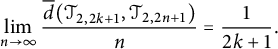 $$\begin{align*}\lim_{n \to \infty} \frac{\overline{d}(\mathcal{T}_{2,2k+1},\mathcal{T}_{2, 2n+1}) }{n} = \frac{1}{2k+1}.\end{align*}$$
Proof By Theorem 2.1, we have that
 $$\begin{align*}\overline{d}( \mathcal{T}_{2,2k+1},\mathcal{T}_{2, 2n+1}) \le \min\{ n - \alpha k , (\alpha +1)(k+1) - n -1 \}, \end{align*}$$
where
 $\alpha = \lfloor \frac {2n+1}{2k+1} \rfloor $
. Since
$\alpha = \lfloor \frac {2n+1}{2k+1} \rfloor $
. Since
 $\big | \alpha - \frac {2n+1}{2k+1} \big | \le 1$
and is not multiplied by n in this bound, we can replace
$\big | \alpha - \frac {2n+1}{2k+1} \big | \le 1$
and is not multiplied by n in this bound, we can replace
 $\alpha $
with
$\alpha $
with
 $\frac {2n+1}{2k+1}$
in the bound without changing the limiting behavior once it is divided by n. An elementary algebraic manipulation then provides the upper bound for the limit of
$\frac {2n+1}{2k+1}$
in the bound without changing the limiting behavior once it is divided by n. An elementary algebraic manipulation then provides the upper bound for the limit of
 $\overline {d}/n$
to be
$\overline {d}/n$
to be
 $\frac {1}{2k+1}$
.
$\frac {1}{2k+1}$
.
To get the lower bound, we use Corollary 3.3, which implies that
 $$\begin{align*}\overline{d}( \mathcal{T}_{2,2k+1},\mathcal{T}_{2, 2n+1})) \ge \lfloor \lfloor \frac{1}{2}\frac{2n+1}{2k+1} +\frac{1}{2} \rfloor\rfloor. \end{align*}$$
Again, the floor function differs from its argument by an amount that bounded by 1, so we have
 $$\begin{align*}\overline{d}( \mathcal{T}_{2,2k+1},\mathcal{T}_{2, 2n+1})) \ge \frac{1}{2}\frac{2n+1}{2k+1} +\frac{1}{2}. \end{align*}$$
Forming the quotient with n and taking the limit as n goes to infinity gives the desired lower bound.
4 Projectivizing abelian groups
We would like to define a distance on the concordance group by something like
 $$\begin{align*}\min \{ d(K, J) \ \big| \ \mathcal{K} \in \mathcal{S}_1, \mathcal{J} \in \mathcal{S}_2 \}, \end{align*}$$
where
 $\mathcal {S}_1$
and
$\mathcal {S}_1$
and
 $\mathcal {S}_2$
are maximal cyclic subgroups of
$\mathcal {S}_2$
are maximal cyclic subgroups of
 $\mathcal {C}$
containing
$\mathcal {C}$
containing
 $\mathcal {K}$
and
$\mathcal {K}$
and
 $\mathcal {J}$
, respectively. Such maximal subgroups exist by Zorn’s Lemma; however, they need not be unique. For example, consider
$\mathcal {J}$
, respectively. Such maximal subgroups exist by Zorn’s Lemma; however, they need not be unique. For example, consider
 ${\mathbb Z} \oplus {\mathbb Z}_2$
. The subgroups
${\mathbb Z} \oplus {\mathbb Z}_2$
. The subgroups
 $\left < (1,0) \right>$
and
$\left < (1,0) \right>$
and
 $\left < (1,1) \right>$
are both maximal cyclic subgroups containing
$\left < (1,1) \right>$
are both maximal cyclic subgroups containing
 $(2,0)$
.
$(2,0)$
.
In this section, we will discuss a general approach to the algebra associated with the relation on a group generated by the property of elements being in a common cyclic subgroup. The construction is modeled on that of projective spaces associated with vector spaces. Although our interest is ultimately in the abelian group
 $\mathcal {C}$
, a
$\mathcal {C}$
, a
 ${\mathbb Z}$
-module, it will be valuable to work with general modules over integral domains.
${\mathbb Z}$
-module, it will be valuable to work with general modules over integral domains.
4.1 The projective space of an R-module
Let R be an integral domain, let M be a left R-module, and let
 $M^\circ = M \setminus 0$
. Define a binary relation on
$M^\circ = M \setminus 0$
. Define a binary relation on
 $M^o$
by
$M^o$
by
 $x \sim ' y$
if there exists an
$x \sim ' y$
if there exists an
 $m\in M$
such that
$m\in M$
such that
 $x = rm$
and
$x = rm$
and
 $y= sm$
for some
$y= sm$
for some
 $r, s \in R$
and some
$r, s \in R$
and some
 $m\in M$
. Notice that this is reflexive and symmetric, but it need not be transitive.
$m\in M$
. Notice that this is reflexive and symmetric, but it need not be transitive.
Example 4.1 Let
 $R = {\mathbb Z}$
and
$R = {\mathbb Z}$
and
 $M= {\mathbb Z} \oplus {\mathbb Z}_2 \oplus {\mathbb Z}_2.$
Then
$M= {\mathbb Z} \oplus {\mathbb Z}_2 \oplus {\mathbb Z}_2.$
Then
 $(1,1,0) \sim ' (2,0,0)$
and
$(1,1,0) \sim ' (2,0,0)$
and
 $(1,0,1) \sim ' (2,0,0)$
, but
$(1,0,1) \sim ' (2,0,0)$
, but
 $(1,1,0) \not \sim ' (1,0,1).$
Definition 4.1 Define the projective relation on
 $M^\circ $
,
$M^\circ $
,
 $x \sim _M y $
, to be the equivalence relation generated by
$x \sim _M y $
, to be the equivalence relation generated by
 $\sim '$
. That is,
$\sim '$
. That is,
 $a \sim _M b$
if and only if there is a finite chain
$a \sim _M b$
if and only if there is a finite chain
 $$\begin{align*}x = x_0 \sim' x_1 \sim' \cdots \sim' x_n = y. \end{align*}$$
Except where needed, we will write “
 $\sim $
” instead of “
$\sim $
” instead of “
 $\sim _M$
.”
$\sim _M$
.”
Definition 4.2 Define the projective space
 ${\mathbb P}( M) = M^\circ /\sim $
. Set
${\mathbb P}( M) = M^\circ /\sim $
. Set
 ${\mathbb P}^*(M) = * \sqcup {\mathbb P}(M)$
, where
${\mathbb P}^*(M) = * \sqcup {\mathbb P}(M)$
, where
 $*$
denotes a disjoint point.
$*$
denotes a disjoint point.
The following result might clarify the equivalence relation and highlights why we chose to define it in terms of having common divisors instead of having common multiples. As we do not use it later, the elementary proof is left to the reader.
Theorem 4.2 If
 $x, y \in M$
are nontorsion elements and
$x, y \in M$
are nontorsion elements and
 $[x] = [y] \in {\mathbb P}(M)$
, then there exist elements
$[x] = [y] \in {\mathbb P}(M)$
, then there exist elements
 $a, b \in R$
such that
$a, b \in R$
such that
 $ax = by \ne 0$
.
$ax = by \ne 0$
.
We conclude this subsection with a few basic examples.
Example 4.3 The classes
 $[2] = [3] \in {\mathbb P}({\mathbb Z}_6)$
have a common divisor, but the two elements
$[2] = [3] \in {\mathbb P}({\mathbb Z}_6)$
have a common divisor, but the two elements
 $2, 3 \in {\mathbb Z}_6$
have no nonzero multiple in common.
$2, 3 \in {\mathbb Z}_6$
have no nonzero multiple in common.
Example 4.4 The projective space
 ${\mathbb P}({\mathbb Z}_2 \oplus {\mathbb Z}_2)$
has three elements corresponding to the three nontrivial elements in the group. On the other hand, an elementary calculation shows that
${\mathbb P}({\mathbb Z}_2 \oplus {\mathbb Z}_2)$
has three elements corresponding to the three nontrivial elements in the group. On the other hand, an elementary calculation shows that
 ${\mathbb P}({\mathbb Z}_2 \oplus {\mathbb Z}_2 \oplus {\mathbb Z}_3)$
has one element.
${\mathbb P}({\mathbb Z}_2 \oplus {\mathbb Z}_2 \oplus {\mathbb Z}_3)$
has one element.
Example 4.5 If
 $R = {\mathbb F}$
is a field, then
$R = {\mathbb F}$
is a field, then
 ${\mathbb P} (M)$
is the standard projective space. For instance, if
${\mathbb P} (M)$
is the standard projective space. For instance, if
 $M = {\mathbb F}^n$
, then
$M = {\mathbb F}^n$
, then
 ${\mathbb P}({\mathbb F}^n) $
is, in the usual notation,
${\mathbb P}({\mathbb F}^n) $
is, in the usual notation,
 ${\mathbb P} {\mathbb F}^{n-1}$
. In Corollary 4.12, we discuss the case that
${\mathbb P} {\mathbb F}^{n-1}$
. In Corollary 4.12, we discuss the case that
 $M = R^n$
for an integral domain R.
$M = R^n$
for an integral domain R.
4.2 Induced maps
$ {\mathbb P}(M) \to {\mathbb P}(N)$

In the next subsection, we will consider the case of torsion abelian groups. In the subsection after that, we present the case of torsion free abelian groups. In the first case, torsion groups can be understood in terms of their elements of prime order. The projectivization of torsion free groups can be understood by moving from
 ${\mathbb Z}$
-modules to
${\mathbb Z}$
-modules to
 ${\mathbb Q}$
-vector spaces. Underlying these changes of domain is the following result, which provides induced maps on projective spaces. The proof is straightforward except for Statement (3), which calls for an example. Such an example is provided by the case of
${\mathbb Q}$
-vector spaces. Underlying these changes of domain is the following result, which provides induced maps on projective spaces. The proof is straightforward except for Statement (3), which calls for an example. Such an example is provided by the case of
 ${\mathbb P}( {\mathbb Z}_2 \oplus {\mathbb Z}_2) \to {\mathbb P}({\mathbb Z}_2 \oplus {\mathbb Z}_2 \oplus {\mathbb Z})$
given in Example 4.4.
${\mathbb P}( {\mathbb Z}_2 \oplus {\mathbb Z}_2) \to {\mathbb P}({\mathbb Z}_2 \oplus {\mathbb Z}_2 \oplus {\mathbb Z})$
given in Example 4.4.
Theorem 4.6 Let M be an R-module, let N be an S-module, let
 $\phi \colon \thinspace R\to S$
be a ring homomorphism, and let
$\phi \colon \thinspace R\to S$
be a ring homomorphism, and let
 $F\colon \thinspace M \to N$
be a module homomorphism over
$F\colon \thinspace M \to N$
be a module homomorphism over
 $\phi $
. Then: (1)
$\phi $
. Then: (1)
 ${\mathbb F}$
induces a map
${\mathbb F}$
induces a map
 $F_*\colon \thinspace {\mathbb P}^*(M) \to {\mathbb P}^*(N)$
, sending the equivalence class of x to
$F_*\colon \thinspace {\mathbb P}^*(M) \to {\mathbb P}^*(N)$
, sending the equivalence class of x to
 $*$
if
$*$
if
 $rx \in \ker (F)$
for some
$rx \in \ker (F)$
for some
 $r \ne 0$
; (2) if F is surjective, then
$r \ne 0$
; (2) if F is surjective, then
 $F_*$
is surjective; and (3) if F is injective, then there is also an induced map
$F_*$
is surjective; and (3) if F is injective, then there is also an induced map
 $F_* \colon \thinspace {\mathbb P}(M) \to {\mathbb P}(N)$
; this map need not be injective.
$F_* \colon \thinspace {\mathbb P}(M) \to {\mathbb P}(N)$
; this map need not be injective.
4.3 Torsion groups
Example 4.7 For any
 $n>1$
,
$n>1$
,
 ${\mathbb P}({\mathbb Z}_n)$
has one point, the equivalence class of
${\mathbb P}({\mathbb Z}_n)$
has one point, the equivalence class of
 $1$
.
$1$
.
Theorem 4.8 If G is a torsion abelian group containing elements a and b of distinct prime orders p and q, then
 ${\mathbb P}(G)$
has one element.
${\mathbb P}(G)$
has one element.
Proof Given an arbitrary
 $x \ne 0 \in G$
, by taking a multiple, we see that x is equivalent to some element
$x \ne 0 \in G$
, by taking a multiple, we see that x is equivalent to some element
 $x'$
of prime order s. Assume that
$x'$
of prime order s. Assume that
 $s \ne q$
. Then
$s \ne q$
. Then
 $$\begin{align*}x' \sim' qx' = q(x'+b) \sim' s(x' +b) = sb \sim' b. \end{align*}$$
Thus, every element is equivalent to either a or b. But these are also equivalent:
 $$\begin{align*}a \sim' qa = q(a +b) \sim' p(a +b) = pb \sim' b. \\[-35pt]\end{align*}$$
Theorem 4.9 Suppose that p is a prime and that each element of an abelian group G has order
 $p^k$
for some k. Let
$p^k$
for some k. Let
 $H \subset G$
be the subgroup consisting of elements x satisfying
$H \subset G$
be the subgroup consisting of elements x satisfying
 $px = 0$
. Then the map induced by inclusion
$px = 0$
. Then the map induced by inclusion
 ${\mathbb P}(H) \to {\mathbb P}(G)$
is a bijection.
${\mathbb P}(H) \to {\mathbb P}(G)$
is a bijection.
Proof Notice that H is a
 ${\mathbb Z}_p$
-vector space and thus each nonzero element lies on a unique line, or stated equivalently, in a unique cyclic subgroup.
${\mathbb Z}_p$
-vector space and thus each nonzero element lies on a unique line, or stated equivalently, in a unique cyclic subgroup.
Given an element
 $x \ne 0 \in G$
, choose the least
$x \ne 0 \in G$
, choose the least
 $n> 0$
such that
$n> 0$
such that
 $nx \in H$
and note
$nx \in H$
and note
 ${nx \ne 0.}$
Denote
${nx \ne 0.}$
Denote
 $nx $
by
$nx $
by
 $F(x)$
. We claim that F induces a bijection
$F(x)$
. We claim that F induces a bijection
 $F_*\colon \thinspace {\mathbb P}(G) \to {\mathbb P}(H)$
.
$F_*\colon \thinspace {\mathbb P}(G) \to {\mathbb P}(H)$
.
First, we show that it is well defined. If
 $x \sim ' y$
, then x and y are in a common cyclic subgroup of G. The intersection of that subgroup with H is a cyclic subgroup, and so
$x \sim ' y$
, then x and y are in a common cyclic subgroup of G. The intersection of that subgroup with H is a cyclic subgroup, and so
 $F(x)$
and
$F(x)$
and
 $F(y)$
lie on a common line in H, which must be the unique line through
$F(y)$
lie on a common line in H, which must be the unique line through
 $F(x)$
. Continuing in this way, if there is a sequence
$F(x)$
. Continuing in this way, if there is a sequence
 $x = x_0 \sim ' x_1\sim ' \cdots \sim ' x_n = y$
, we see that
$x = x_0 \sim ' x_1\sim ' \cdots \sim ' x_n = y$
, we see that
 $F(x_i)$
lies on the line through
$F(x_i)$
lies on the line through
 $F(x)$
for all i and in particular
$F(x)$
for all i and in particular
 $F(x)$
and
$F(x)$
and
 $F(y)$
lie in a common cyclic subgroup. Thus,
$F(y)$
lie in a common cyclic subgroup. Thus,
 $F^*$
is well defined.
$F^*$
is well defined.
It is clear that
 $F_*$
is surjective.
$F_*$
is surjective.
For injectivity, first, note that it is evident that if
 $F(x) \sim _H F(y)$
, then
$F(x) \sim _H F(y)$
, then
 $F(x) \sim _G F(y)$
. It is also clear that
$F(x) \sim _G F(y)$
. It is also clear that
 $F(x) \sim _G x$
and
$F(x) \sim _G x$
and
 $F(y) \sim _G y$
. So, if
$F(y) \sim _G y$
. So, if
 $F(x) \sim _H F(y)$
, we have the chain
$F(x) \sim _H F(y)$
, we have the chain
 $$\begin{align*}x \sim^{\prime}_G F(x) \sim^{\prime}_G F(y) \sim' y.\\[-35pt] \end{align*}$$
Example 4.10 For direct sums, infinite as well as finite, and for any prime p, the inclusion
 $\oplus _i {\mathbb Z}_{p} \to \oplus _i {\mathbb Z}_{p^{a_i}}$
induces a bijection
$\oplus _i {\mathbb Z}_{p} \to \oplus _i {\mathbb Z}_{p^{a_i}}$
induces a bijection
 ${\mathbb P}(\oplus _i {\mathbb Z}_{p}) \to {\mathbb P}(\oplus _i {\mathbb Z}_{p^{a_i}})$
. The domain is a
${\mathbb P}(\oplus _i {\mathbb Z}_{p}) \to {\mathbb P}(\oplus _i {\mathbb Z}_{p^{a_i}})$
. The domain is a
 ${\mathbb Z}_p$
-projective space. There is one point in
${\mathbb Z}_p$
-projective space. There is one point in
 ${\mathbb P}(\oplus _i {\mathbb Z}_p)$
for each order p cyclic subgroup.
${\mathbb P}(\oplus _i {\mathbb Z}_p)$
for each order p cyclic subgroup.
In the case of
 $p=2$
, cyclic subgroups correspond to nontrivial elements of
$p=2$
, cyclic subgroups correspond to nontrivial elements of
 ${\mathbb P}(\oplus _i {\mathbb Z}_2)$
and thus there is a bijection
${\mathbb P}(\oplus _i {\mathbb Z}_2)$
and thus there is a bijection
 $( \oplus _i {\mathbb Z}_2 \setminus 0 ) \to {\mathbb P}(\oplus _i {\mathbb Z}_{2^a_i})$
.
$( \oplus _i {\mathbb Z}_2 \setminus 0 ) \to {\mathbb P}(\oplus _i {\mathbb Z}_{2^a_i})$
.
In the case of a finite sum,
 $ \oplus _{i=0}^n {\mathbb Z}_{p^{a_i}}$
, we have that the number of elements in the projective space is
$ \oplus _{i=0}^n {\mathbb Z}_{p^{a_i}}$
, we have that the number of elements in the projective space is
 $(p^n -1)/(p-1)$
.
$(p^n -1)/(p-1)$
.
4.4 The torsion-free case
Let M be a torsion-free module over R, and let
 ${\mathbb Q}(R)$
denote the field of fractions. Let
${\mathbb Q}(R)$
denote the field of fractions. Let
 $M_{\mathbb Q} = M \otimes {\mathbb Q}(R)$
be the associated
$M_{\mathbb Q} = M \otimes {\mathbb Q}(R)$
be the associated
 ${\mathbb Q}(R)$
vector space.
${\mathbb Q}(R)$
vector space.
Theorem 4.11 If M is torsion-free, then there is a natural bijection
 ${\mathbb P}(M) \to {\mathbb P} (M_{\mathbb Q})$
.
${\mathbb P}(M) \to {\mathbb P} (M_{\mathbb Q})$
.
Proof We first recall the elementary fact that M is torsion-free implies that
 ${M \to M_{\mathbb Q}}$
is injective. Another elementary observation is that for every
${M \to M_{\mathbb Q}}$
is injective. Another elementary observation is that for every
 $x \ne 0 \in M_{\mathbb Q}$
, there is an
$x \ne 0 \in M_{\mathbb Q}$
, there is an
 $ \alpha \ne 0 \in R$
such that
$ \alpha \ne 0 \in R$
such that
 $\alpha x \in M$
. By Theorem 4.6, there is a natural map
$\alpha x \in M$
. By Theorem 4.6, there is a natural map
 $\psi \colon \thinspace {\mathbb P}(M) \to {\mathbb P} (M_{\mathbb Q})$
.
$\psi \colon \thinspace {\mathbb P}(M) \to {\mathbb P} (M_{\mathbb Q})$
.
It is clear that
 $\psi $
is surjective:
$\psi $
is surjective:
 $m \otimes \frac {a}{b} \sim ' b( m \otimes \frac {a}{b} ) = m \otimes a = am \otimes 1$
.
$m \otimes \frac {a}{b} \sim ' b( m \otimes \frac {a}{b} ) = m \otimes a = am \otimes 1$
.
To show that
 $\psi $
is injective, suppose that
$\psi $
is injective, suppose that
 $a, b \in M$
and
$a, b \in M$
and
 $a \sim _{M_{\mathbb Q}} b$
. Then there are an
$a \sim _{M_{\mathbb Q}} b$
. Then there are an
 $r, s \in {\mathbb Q}(R)$
and an
$r, s \in {\mathbb Q}(R)$
and an
 $m \in M_{\mathbb Q}$
such that
$m \in M_{\mathbb Q}$
such that
 $a= rm$
and
$a= rm$
and
 $b=sm$
. Choose an element in
$b=sm$
. Choose an element in
 $t \in R$
such that
$t \in R$
such that
 $tr \in R$
,
$tr \in R$
,
 $ts\in R$
, and
$ts\in R$
, and
 $tm \in M$
. Then we have the following relations in M, where each element within parentheses is in R or M.
$tm \in M$
. Then we have the following relations in M, where each element within parentheses is in R or M.
 $$\begin{align*}a \sim^{\prime}_M (t^2)a =(t^2)(rm) = (tr)(tm) \sim^{\prime}_M (tm) \sim^{\prime}_M (ts)(tm) = (t^2)(sm) = (t^2)b \sim' b. \end{align*}$$
Corollary 4.12 The inclusion
 ${\mathbb Z} \to {\mathbb Q}$
induces a bijection
${\mathbb Z} \to {\mathbb Q}$
induces a bijection
 ${\mathbb P}({\mathbb Z}^\infty ) \to {\mathbb P}({\mathbb Q}^\infty )= {\mathbb Q}{\mathbb P}^\infty $
.
${\mathbb P}({\mathbb Z}^\infty ) \to {\mathbb P}({\mathbb Q}^\infty )= {\mathbb Q}{\mathbb P}^\infty $
.
4.5 Modules with free parts and torsion
We continue to assume that R is an integral domain.
Theorem 4.13 For arbitrary nonzero elements a and b in an R-module M, if
 $a \sim b$
and a is R-torsion, then b is also R-torsion.
$a \sim b$
and a is R-torsion, then b is also R-torsion.
Proof If
 $a \sim ' b$
, then there are an m, r, and s so that
$a \sim ' b$
, then there are an m, r, and s so that
 $a = rm$
and
$a = rm$
and
 $b = sm$
. There is an
$b = sm$
. There is an
 $\alpha \in R$
such that
$\alpha \in R$
such that
 $\alpha \ne 0$
and
$\alpha \ne 0$
and
 $\alpha a = 0$
. Thus,
$\alpha a = 0$
. Thus,
 $\alpha r m = 0$
. We then have that
$\alpha r m = 0$
. We then have that
 $\alpha r b = \alpha r sm =0$
. Since
$\alpha r b = \alpha r sm =0$
. Since
 $\alpha \ne 0 $
,
$\alpha \ne 0 $
,
 $r \ne 0$
, and R is an integral domain, it follows that
$r \ne 0$
, and R is an integral domain, it follows that
 $\alpha r \ne 0$
. Thus, b is also torsion.
$\alpha r \ne 0$
. Thus, b is also torsion.
Finally, we see that in any sequence
 $$\begin{align*}a = x_0 \sim' x_1 \sim' \cdots \sim' x_n = b, \end{align*}$$
each successive
 $x_i$
is torsion.
$x_i$
is torsion.
Let
 $\text {Tor}(M)$
denote the R-torsion submodule in the R-module M.
$\text {Tor}(M)$
denote the R-torsion submodule in the R-module M.
Theorem 4.14 If
 $x \in M$
is not R-torsion and
$x \in M$
is not R-torsion and
 $y \in M$
is R-torsion, then
$y \in M$
is R-torsion, then
 $[x] = [x+y] \in {\mathbb P} (M)$
.
$[x] = [x+y] \in {\mathbb P} (M)$
.
Proof Suppose that
 $r \ne 0$
and
$r \ne 0$
and
 $r y = 0$
. Then
$r y = 0$
. Then
 $0 \ne rx = r(x +y)$
and
$0 \ne rx = r(x +y)$
and
 $$\begin{align*}x \sim' rx = r(x +y) \sim' x+y.\\[-32pt] \end{align*}$$
Theorem 4.15 For any R-module M,
 ${\mathbb P} (M) = {\mathbb P}(\mathrm {Tor}(M)) \bigsqcup {\mathbb P}(M /\mathrm {Tor}(M))$
, where
${\mathbb P} (M) = {\mathbb P}(\mathrm {Tor}(M)) \bigsqcup {\mathbb P}(M /\mathrm {Tor}(M))$
, where
 $\bigsqcup $
denotes disjoint union.
$\bigsqcup $
denotes disjoint union.
Proof Let
 ${\mathbb T}(M) $
denote the set of classes in
${\mathbb T}(M) $
denote the set of classes in
 ${\mathbb P}(M)$
that are represented by elements in
${\mathbb P}(M)$
that are represented by elements in
 $ \mathrm {Tor}(M)$
, and let
$ \mathrm {Tor}(M)$
, and let
 ${\mathbb F}(M)$
consist classes in
${\mathbb F}(M)$
consist classes in
 ${\mathbb P}(M)$
that are represented by nontorsion elements of M. If follows from Theorem 4.13 that
${\mathbb P}(M)$
that are represented by nontorsion elements of M. If follows from Theorem 4.13 that
 ${\mathbb P}(M) = {\mathbb T}(M) \bigsqcup {\mathbb F}(M)$
. Thus, we want to show that
${\mathbb P}(M) = {\mathbb T}(M) \bigsqcup {\mathbb F}(M)$
. Thus, we want to show that
 ${\mathbb P}(\mathrm {Tor}(M)) = {\mathbb T}(M)$
and
${\mathbb P}(\mathrm {Tor}(M)) = {\mathbb T}(M)$
and
 ${\mathbb P}(M / \mathrm {Tor}(M)) = {\mathbb F}(M)$
.
${\mathbb P}(M / \mathrm {Tor}(M)) = {\mathbb F}(M)$
.
Step 1. Consider
 $a, b \in \mathrm {Tor}(M)$
. We first want to show that if
$a, b \in \mathrm {Tor}(M)$
. We first want to show that if
 $a \sim _M b$
, then
$a \sim _M b$
, then
 $a \sim _{\mathrm {Tor}(M)} b$
. Suppose that
$a \sim _{\mathrm {Tor}(M)} b$
. Suppose that
 $$\begin{align*}a = x_0 \sim^{\prime}_M x_1 \sim^{\prime}_M \cdots \sim^{\prime}_M x_n = b \end{align*}$$
is a chain. We first note that each
 $x_i \in {\mathrm {Tor}(M)} $
. If
$x_i \in {\mathrm {Tor}(M)} $
. If
 $a = rm $
and
$a = rm $
and
 $x_1 = sm$
, then since a is torsion, m is also torsion, and thus
$x_1 = sm$
, then since a is torsion, m is also torsion, and thus
 $x_1$
is torsion. Proceed by induction.
$x_1$
is torsion. Proceed by induction.
We now need to show that if
 $a, b \in {\mathrm {Tor}(M)} $
and
$a, b \in {\mathrm {Tor}(M)} $
and
 $a \sim ^{\prime }_M b$
, then
$a \sim ^{\prime }_M b$
, then
 $a \sim ^{\prime }_{\mathrm {Tor}(M)} b$
. Again, if
$a \sim ^{\prime }_{\mathrm {Tor}(M)} b$
. Again, if
 $a = rm $
and
$a = rm $
and
 $b = sm$
, then since a is torsion, m is also torsion, and thus a and b are multiples of a common element in
$b = sm$
, then since a is torsion, m is also torsion, and thus a and b are multiples of a common element in
 ${\mathrm {Tor}(M)}$
.
${\mathrm {Tor}(M)}$
.
Step 2. We now observe that the previous step implies that
 ${\mathbb P}( \mathrm {Tor}(M)) = {\mathbb T}(M) $
. The inclusion
${\mathbb P}( \mathrm {Tor}(M)) = {\mathbb T}(M) $
. The inclusion
 $\mathrm {Tor}(M) \to M$
induces a map
$\mathrm {Tor}(M) \to M$
induces a map
 ${\mathbb P}( \mathrm {Tor}(M)) \to {\mathbb T}(M)$
. It is clearly surjective, and the previous step shows that it is injective.
${\mathbb P}( \mathrm {Tor}(M)) \to {\mathbb T}(M)$
. It is clearly surjective, and the previous step shows that it is injective.
Step 3. We now want to understand
 ${\mathbb F}(M)$
. Define
${\mathbb F}(M)$
. Define
 $\phi \colon \thinspace {\mathbb F}(M) \to {\mathbb P}(M /\mathrm {Tor}(M))$
by
$\phi \colon \thinspace {\mathbb F}(M) \to {\mathbb P}(M /\mathrm {Tor}(M))$
by
 $[a]\to [\overline {a}]$
, where
$[a]\to [\overline {a}]$
, where
 $\overline {a}$
is the image of a in
$\overline {a}$
is the image of a in
 $M / \mathrm {Tor}(M)$
. It is clear that
$M / \mathrm {Tor}(M)$
. It is clear that
 $\phi $
is well defined: if
$\phi $
is well defined: if
 $[a] = [a']$
, then
$[a] = [a']$
, then
 $\overline {a} \ne 0 \ne \overline {a}'$
and
$\overline {a} \ne 0 \ne \overline {a}'$
and
 $ [\overline {a}] = [\overline {a}']$
. It is also clear that
$ [\overline {a}] = [\overline {a}']$
. It is also clear that
 $\phi $
is surjective.
$\phi $
is surjective.
We now prove injectivity. If
 $\overline {a} \sim ' \overline {b}$
, then there are an element
$\overline {a} \sim ' \overline {b}$
, then there are an element
 $m \in M$
, elements
$m \in M$
, elements
 $r, s \in R$
, and torsion elements
$r, s \in R$
, and torsion elements
 $t_1, t_2 \in \mathrm {Tor}(M)$
such that
$t_1, t_2 \in \mathrm {Tor}(M)$
such that
 $a +t_1 = rm$
and
$a +t_1 = rm$
and
 $b +t_2 = sm$
. Suppose that
$b +t_2 = sm$
. Suppose that
 $\alpha \in R$
satisfies
$\alpha \in R$
satisfies
 $\alpha t_1 = 0 = \alpha t_2$
. Then
$\alpha t_1 = 0 = \alpha t_2$
. Then
 $\alpha a = \alpha r m$
and
$\alpha a = \alpha r m$
and
 $\alpha b = \alpha s m$
. We then have the chain
$\alpha b = \alpha s m$
. We then have the chain
 $$\begin{align*}a \sim' \alpha a \sim'm \sim'\alpha b \sim' b.\\[-37pt] \end{align*}$$
4.6 The projectivization of the concordance group:
${\mathbb P}(\mathcal {C})$

We have the decomposition
 ${\mathbb P}(\mathcal {C}) = {\mathbb P}({\text {Tor}}(\mathcal {C})) \sqcup {\mathbb P}(\mathcal {C}/{\text {Tor}}(\mathcal {C}))$
.
${\mathbb P}(\mathcal {C}) = {\mathbb P}({\text {Tor}}(\mathcal {C})) \sqcup {\mathbb P}(\mathcal {C}/{\text {Tor}}(\mathcal {C}))$
.
By Theorem 4.11, we have that
 ${\mathbb P}(\mathcal {C}/{\text {Tor}}(\mathcal {C}))$
is in bijective correspondence with
${\mathbb P}(\mathcal {C}/{\text {Tor}}(\mathcal {C}))$
is in bijective correspondence with
 ${\mathbb P}(V)$
for some
${\mathbb P}(V)$
for some
 ${\mathbb Q}$
-vector space. Also,
${\mathbb Q}$
-vector space. Also,
 $\mathcal {C}$
contains an infinite linearly independent set, so if fact,
$\mathcal {C}$
contains an infinite linearly independent set, so if fact,
 ${\mathbb P}(\mathcal {C}/{\text {Tor}}(\mathcal {C}))$
is in bijective correspondence with
${\mathbb P}(\mathcal {C}/{\text {Tor}}(\mathcal {C}))$
is in bijective correspondence with
 ${\mathbb P}({\mathbb Q}^\infty )$
.
${\mathbb P}({\mathbb Q}^\infty )$
.
Since
 $\mathcal {C}$
contains 2-torsion, if it also contains torsion of odd order, then by Theorem 4.8,
$\mathcal {C}$
contains 2-torsion, if it also contains torsion of odd order, then by Theorem 4.8,
 ${\mathbb P}(\mathcal {C}/{\text {Tor}}(\mathcal {C}))$
has one point. On the other hand, if all elements are of order
${\mathbb P}(\mathcal {C}/{\text {Tor}}(\mathcal {C}))$
has one point. On the other hand, if all elements are of order
 $2^k$
for some k, then by Theorem 4.9, we have
$2^k$
for some k, then by Theorem 4.9, we have
 ${\mathbb P}(\mathcal {C}/{\text {Tor}}(\mathcal {C}))$
is in bijective correspondence with
${\mathbb P}(\mathcal {C}/{\text {Tor}}(\mathcal {C}))$
is in bijective correspondence with
 ${\mathbb P}({\mathbb Z}_2^\infty )$
. We summarize these observations with the following theorem.
${\mathbb P}({\mathbb Z}_2^\infty )$
. We summarize these observations with the following theorem.
Theorem 4.16 Either
 $ {\mathbb P}(\mathcal {C}) = {\mathbb P}(Z_2^\infty ) \sqcup {\mathbb P}({\mathbb Q}^\infty )$
or
$ {\mathbb P}(\mathcal {C}) = {\mathbb P}(Z_2^\infty ) \sqcup {\mathbb P}({\mathbb Q}^\infty )$
or
 $ {\mathbb P}(\mathcal {C}) = {*} \sqcup {\mathbb P}({\mathbb Q}^\infty )$
, where
$ {\mathbb P}(\mathcal {C}) = {*} \sqcup {\mathbb P}({\mathbb Q}^\infty )$
, where
 $*$
is a single point. The first case holds if
$*$
is a single point. The first case holds if
 $\mathcal {C}$
contains no odd order torsion. The second case holds if there is odd torsion.
$\mathcal {C}$
contains no odd order torsion. The second case holds if there is odd torsion.
5 Metrics on
${\mathbb P}^*(M)$

Suppose that d is an integer-valued metric on the module M. We show that it induces a metric
 $\Delta $
on
$\Delta $
on
 ${\mathbb P}^*(M)$
.
${\mathbb P}^*(M)$
.
5.1 Definition of
$\Delta $
.

Recall that for an element
 $x \in M$
, we denote its equivalence class by
$x \in M$
, we denote its equivalence class by
 $[x]\in {\mathbb P}^*(M)$
. Also,
$[x]\in {\mathbb P}^*(M)$
. Also,
 $0 \in M$
is the unique representative of the class we have denoted
$0 \in M$
is the unique representative of the class we have denoted
 $*$
.
$*$
.
Definition 5.1
-
(1) For
$[x] \in {\mathbb P}^*(M)$
and
$ [y] \in {\mathbb P}^*(M) $
,
$$\begin{align*}\delta ([x],[ y]) = \inf \{ d(x',y') \ \big| \ x' \in [x]\ ,\ y' \in [y]\}.\end{align*}$$
-
(2) For
$[x] \in {\mathbb P}^*(M)$
and
$ [y] \in {\mathbb P}^*(M) $
, where the minimum is taken over all sequences of classes for which
$$\begin{align*}\Delta([ x],[y ]) = \min\{\delta( [x_0],[ x_1 ])+ \delta( [x_1],[ x_2] ) + \cdots + \delta( [x_{n-1}], [x_n ])\}, \end{align*}$$
$[x_0] =[ x]$
and
$[x_n] =[ y]$
.


Elementary examples demonstrate the need of considering chains to achieve transitivity. The proof of the following result is immediate, given that d is integer-valued.
Theorem 5.1 The function
 $\Delta \colon \thinspace {\mathbb P}^*(M) \times {\mathbb P}^*(M) \to {\mathbb Z}$
is a metric.
$\Delta \colon \thinspace {\mathbb P}^*(M) \times {\mathbb P}^*(M) \to {\mathbb Z}$
is a metric.
5.2 Mappings of metric spaces
$({\mathbb P}^*(M), \Delta )$
.

Definition 5.2 Suppose that
 $F\colon \thinspace (X,d) \to (Y,d')$
is a function between metric spaces. Then F is called a weak contraction if
$F\colon \thinspace (X,d) \to (Y,d')$
is a function between metric spaces. Then F is called a weak contraction if
 $d'(F(x_0), F(x_1)) \le d(x_0,x_1)$
for all
$d'(F(x_0), F(x_1)) \le d(x_0,x_1)$
for all
 $x_0$
and
$x_0$
and
 $x_1$
in X.
$x_1$
in X.
We have the following elementary result.
Theorem 5.2 If
 $F \colon \thinspace (M,d) \to (N,d')$
is a weak contraction of modules with integer valued metrics, then
$F \colon \thinspace (M,d) \to (N,d')$
is a weak contraction of modules with integer valued metrics, then
 $F_*\colon \thinspace ({\mathbb P}^*(M),\Delta ) \to ({\mathbb P}^*(N), \Delta ')$
is a weak contraction with respect to the induced metrics.
$F_*\colon \thinspace ({\mathbb P}^*(M),\Delta ) \to ({\mathbb P}^*(N), \Delta ')$
is a weak contraction with respect to the induced metrics.
6 Properties of the metric
$\Delta $
on
${\mathbb P}^*(\mathcal {C})$


Here is the definition of the metric
 $\Delta $
restated for the special case of knots.
$\Delta $
restated for the special case of knots.
Definition 6.1
-
(1) For
$\mathcal {K}$
and
$ \mathcal {J} $
in
$ \mathcal {C}$
,
$d(\mathcal {K}, \mathcal {J}) = d(K, J) = g_4(K \mathbin {\#} -J)$
, where K and J are arbitrary representatives of
$\mathcal {K}$
and
$\mathcal {J}$
. -
(2) For
$[\mathcal {K}] \in {\mathbb P}(\mathcal {C})$
and
$ [\mathcal {J}] \in {\mathbb P}(\mathcal {C}) $
,
$$\begin{align*}\delta ([\mathcal{K}],[ \mathcal{J}]) = \min \{ d(\mathcal{K}', \mathcal{J}') \ \big| \ \mathcal{K}' \in [\mathcal{K}]\ ,\ \mathcal{J}' \in [\mathcal{J}]\}.\end{align*}$$
-
(3) For
$[\mathcal {K}] \in {\mathbb P}(\mathcal {C})$
and
$ [\mathcal {J}] \in {\mathbb P}(\mathcal {C}) $
, where the minimum is taken over all sequences of classes for which
$$\begin{align*}\Delta([ \mathcal{K}],[ \mathcal{J} ]) = \min\{\delta( [\mathcal{K}_0],[ \mathcal{K}_1 ])+ \delta( [\mathcal{K}_1],[ \mathcal{K}_2] ) + \cdots + \delta( [\mathcal{K}_{n-1}], [\mathcal{K}_n ])\}, \end{align*}$$
$[\mathcal {K}_0] =[ \mathcal {K}]$
and
$[\mathcal {K}_n] =[ \mathcal {J}]$
.


Here is a consequence of Theorem 4.2 relating the metric
 $\Delta $
to linear independence in
$\Delta $
to linear independence in
 $\mathcal {C}$
.
$\mathcal {C}$
.
Theorem 6.1 If
 $\mathcal {K}$
and
$\mathcal {K}$
and
 $\mathcal {J}$
are elements of infinite order in
$\mathcal {J}$
are elements of infinite order in
 $\mathcal {C}$
, then
$\mathcal {C}$
, then
 $\Delta (\mathcal {K}, \mathcal {J}) = 0$
implies that there are
$\Delta (\mathcal {K}, \mathcal {J}) = 0$
implies that there are
 $a, b \in {\mathbb Z}$
such that
$a, b \in {\mathbb Z}$
such that
 $a\mathcal {K} = b\mathcal {J} \ne 0$
.
$a\mathcal {K} = b\mathcal {J} \ne 0$
.
Example 4.3 demonstrates that if
 $\mathcal {C}$
contains an element of odd order, then the converse does not generalize to the case of knots of finite order. On the other hand, if
$\mathcal {C}$
contains an element of odd order, then the converse does not generalize to the case of knots of finite order. On the other hand, if
 $\mathcal {C} \cong {\mathbb Z}_2^\infty \oplus {\mathbb Z}^\infty $
as might be conjectured, then the condition that
$\mathcal {C} \cong {\mathbb Z}_2^\infty \oplus {\mathbb Z}^\infty $
as might be conjectured, then the condition that
 $\mathcal {K}$
and
$\mathcal {K}$
and
 $\mathcal {J}$
are of infinite order could be dropped.
$\mathcal {J}$
are of infinite order could be dropped.
Another elementary result is the following.
Theorem 6.2
(1)
 $\Delta (\mathcal {K}, \mathcal {J}) = 1$
if and only if
$\Delta (\mathcal {K}, \mathcal {J}) = 1$
if and only if
 $\delta (\mathcal {K}, \mathcal {J}) = 1$
. (2) If
$\delta (\mathcal {K}, \mathcal {J}) = 1$
. (2) If
 $\delta (\mathcal {K}, \mathcal {J}) = 2$
, then
$\delta (\mathcal {K}, \mathcal {J}) = 2$
, then
 $\Delta (\mathcal {K}, \mathcal {J}) = 2$
.
$\Delta (\mathcal {K}, \mathcal {J}) = 2$
.
Here is one topological result concerning
 $\Delta ([ \mathcal {K} ], [\mathcal {J}])$
.
$\Delta ([ \mathcal {K} ], [\mathcal {J}])$
.
Theorem 6.3 If
 $\Delta ([\mathcal {K}], [\mathcal {J}]) = n>0 $
, then there exists a sequence
$\Delta ([\mathcal {K}], [\mathcal {J}]) = n>0 $
, then there exists a sequence
 $\mathcal {K} = \mathcal {K}_0 , \mathcal {K}_1, \ldots , \mathcal {K}_n = \mathcal {J}$
such that for
$\mathcal {K} = \mathcal {K}_0 , \mathcal {K}_1, \ldots , \mathcal {K}_n = \mathcal {J}$
such that for
 $0 \le i \le n-1$
,
$0 \le i \le n-1$
,
 $\delta (\mathcal {K}_i , \mathcal {K}_{i+1}) = 1 $
.
$\delta (\mathcal {K}_i , \mathcal {K}_{i+1}) = 1 $
.
Proof We work with
 $\delta $
and prove the analogous statement. This clearly implies the result for
$\delta $
and prove the analogous statement. This clearly implies the result for
 $\Delta $
. Thus, assume that
$\Delta $
. Thus, assume that
 $\delta ([\mathcal {K}], [\mathcal {J}]) = n>0 $
. Then there exist representative knots
$\delta ([\mathcal {K}], [\mathcal {J}]) = n>0 $
. Then there exist representative knots
 $K' \in [\mathcal {K}]$
and
$K' \in [\mathcal {K}]$
and
 $J' \in [\mathcal {J}]$
for which
$J' \in [\mathcal {J}]$
for which
 $d(K', J') = n$
.
$d(K', J') = n$
.
Let C be a genus n cobordism from
 $K'$
to
$K'$
to
 $J'$
. An isotopy can be performed so that the maximums all occur first and the minimum last. Call the count of these M and N. The saddle points can be put in arbitrary order, the count of these will call S. From the Euler characteristic, we know that genus of the cobordism satisfies
$J'$
. An isotopy can be performed so that the maximums all occur first and the minimum last. Call the count of these M and N. The saddle points can be put in arbitrary order, the count of these will call S. From the Euler characteristic, we know that genus of the cobordism satisfies
 $n = (S - M -N)/2$
.
$n = (S - M -N)/2$
.
By ordering the saddle points, we can arrange that the first N saddle points create a genus 0 cobordism, a concordance, between
 $K'$
and a knot
$K'$
and a knot
 $K"$
. That is, after the maximum are passed, there are
$K"$
. That is, after the maximum are passed, there are
 $N+1$
components, and the first N saddle points reconnect the curve. Similarly, the remaining saddle points can be paired so that the last ones along with the minimums form a concordance from
$N+1$
components, and the first N saddle points reconnect the curve. Similarly, the remaining saddle points can be paired so that the last ones along with the minimums form a concordance from
 $J'$
to a knot
$J'$
to a knot
 $J"$
.
$J"$
.
We are now left with a cobordism of genus n from
 $K"$
to
$K"$
to
 $J"$
containing only saddle points. Those saddle points can now be ordered to form a set of
$J"$
containing only saddle points. Those saddle points can now be ordered to form a set of
 $(S-M-N)$
pairs: the first of each pair disconnects the curve, and the second reconnects them. Thus, we have built a cobordism that consists of a sequence of cobordisms, each of genus 1. The knots formed in this process constitute the desired knots
$(S-M-N)$
pairs: the first of each pair disconnects the curve, and the second reconnects them. Thus, we have built a cobordism that consists of a sequence of cobordisms, each of genus 1. The knots formed in this process constitute the desired knots
 $K_i$
.
$K_i$
.
7 Computation the projective distance
In general, computing the projective distance
 $\delta ([\mathcal {K}],[ \mathcal {J}])$
is inaccessible, and computing
$\delta ([\mathcal {K}],[ \mathcal {J}])$
is inaccessible, and computing
 $\Delta $
is even more difficult. For instance, if
$\Delta $
is even more difficult. For instance, if
 $\mathcal {C}$
contains elements that are infinitely divisible, it is hard to imagine what tools could effectively measure the distance between all divisors for a pair of such knots. Thus, we will want to restrict ourselves to knots that are primitive, using an additive function to do so, and then use perhaps other additive functions to bound the distance.
$\mathcal {C}$
contains elements that are infinitely divisible, it is hard to imagine what tools could effectively measure the distance between all divisors for a pair of such knots. Thus, we will want to restrict ourselves to knots that are primitive, using an additive function to do so, and then use perhaps other additive functions to bound the distance.
We begin with an elementary observation and move to Theorem 7.3, which provides a tool in our computations of
 $\delta $
. In the next section, we consider the metric
$\delta $
. In the next section, we consider the metric
 $\Delta $
.
$\Delta $
.
Theorem 7.1 Let
 $\nu \colon \thinspace \mathcal {C} \to {\mathbb Z}$
and
$\nu \colon \thinspace \mathcal {C} \to {\mathbb Z}$
and
 $\psi \colon \thinspace \mathcal {C} \to {\mathbb R}$
be additive functions. If
$\psi \colon \thinspace \mathcal {C} \to {\mathbb R}$
be additive functions. If
 $\nu (\mathcal {K}) = 1$
, then for all
$\nu (\mathcal {K}) = 1$
, then for all
 $\mathcal {K}' \in [\mathcal {K}]$
,
$\mathcal {K}' \in [\mathcal {K}]$
,
 $\psi (\mathcal {K}') = \nu (\mathcal {K}') \psi ( \mathcal {K})$
.
$\psi (\mathcal {K}') = \nu (\mathcal {K}') \psi ( \mathcal {K})$
.
Proof If we simplify the condition that
 $\nu (\mathcal {K}) = 1$
to
$\nu (\mathcal {K}) = 1$
to
 $\nu (\mathcal {K}) \ne 0$
, it is clear from the definition of
$\nu (\mathcal {K}) \ne 0$
, it is clear from the definition of
 $\sim '$
that if
$\sim '$
that if
 $\mathcal {K} \sim ' \mathcal {K}'$
, then
$\mathcal {K} \sim ' \mathcal {K}'$
, then
 $(\nu (\mathcal {K}'), \psi (\mathcal {K}')) = c (\nu (\mathcal {K}), \psi (\mathcal {K}))$
for some
$(\nu (\mathcal {K}'), \psi (\mathcal {K}')) = c (\nu (\mathcal {K}), \psi (\mathcal {K}))$
for some
 $c \ne 0 \in {\mathbb Q}$
. Thus, it quickly follows that if
$c \ne 0 \in {\mathbb Q}$
. Thus, it quickly follows that if
 $\mathcal {K} \sim \mathcal {K}'$
, we also have
$\mathcal {K} \sim \mathcal {K}'$
, we also have
 $(\nu (\mathcal {K}'), \psi (\mathcal {K}')) = c (\nu (\mathcal {K}), \psi (\mathcal {K}))$
for some
$(\nu (\mathcal {K}'), \psi (\mathcal {K}')) = c (\nu (\mathcal {K}), \psi (\mathcal {K}))$
for some
 $c \ne 0 \in {\mathbb Q}$
. Applying the condition that
$c \ne 0 \in {\mathbb Q}$
. Applying the condition that
 $\nu (\mathcal {K}) = 1$
gives the desired result.
$\nu (\mathcal {K}) = 1$
gives the desired result.
Theorem 7.2 Let
 $\nu _1\colon \thinspace \mathcal {C} \to {\mathbb Z}$
and
$\nu _1\colon \thinspace \mathcal {C} \to {\mathbb Z}$
and
 $\nu _2 \colon \thinspace \mathcal {C} \to {\mathbb Z}$
be additive functions, and let
$\nu _2 \colon \thinspace \mathcal {C} \to {\mathbb Z}$
be additive functions, and let
 $\psi \colon \thinspace \mathcal {C} \to {\mathbb R}$
be an additive function satisfying
$\psi \colon \thinspace \mathcal {C} \to {\mathbb R}$
be an additive function satisfying
 $\big | \psi (\mathcal {K}) \big | \le g_4(\mathcal {K})$
for all
$\big | \psi (\mathcal {K}) \big | \le g_4(\mathcal {K})$
for all
 $\mathcal {K} \in \mathcal {C}$
. Suppose that
$\mathcal {K} \in \mathcal {C}$
. Suppose that
 $\nu _1(\mathcal {K}) = 1$
and
$\nu _1(\mathcal {K}) = 1$
and
 $\nu _2(\mathcal {J}) = 1$
. Then
$\nu _2(\mathcal {J}) = 1$
. Then
 $$\begin{align*}\delta([\mathcal{K}],[ \mathcal{J}]) \ge \min\{ \psi(a\mathcal{K} \mathbin{\#} -b\mathcal{J})\ \big| \ a, b \ne 0\}. \end{align*}$$
Let
 $\Omega $
denote a set of real-valued additive invariants on the concordance group that give lower bounds on the four-genus. Let
$\Omega $
denote a set of real-valued additive invariants on the concordance group that give lower bounds on the four-genus. Let
 $\nu _1$
and
$\nu _1$
and
 $\nu _2$
be
$\nu _2$
be
 ${\mathbb Z}$
-valued additive invariants. The following is now immediate.
${\mathbb Z}$
-valued additive invariants. The following is now immediate.
Theorem 7.3 Suppose that
 $\nu _1(\mathcal {K}) = 1$
and
$\nu _1(\mathcal {K}) = 1$
and
 $\nu _2(\mathcal {J}) = 1$
. Then
$\nu _2(\mathcal {J}) = 1$
. Then
 $$\begin{align*}\delta([\mathcal{K}],[\mathcal{J}]) \ge \min \big\{ | \max\{ \big |a\psi(\mathcal{K}) - b\psi(\mathcal{J}) | \ \big| \ \psi \in \Omega \}\ \big| \ a \in {\mathbb Z}, b\in {\mathbb Z}, ab \ne 0 \big\}. \end{align*}$$
Example 7.4 We apply Theorem 7.2 to show that
 $\delta ([\mathcal {T}_{2,3}],[\mathcal {T}_{2,13}] )= 2$
.
$\delta ([\mathcal {T}_{2,3}],[\mathcal {T}_{2,13}] )= 2$
.
Let
 $\nu _1(K) = \sigma ^{\prime }_*(\frac {1}{3} +\epsilon )$
, and let
$\nu _1(K) = \sigma ^{\prime }_*(\frac {1}{3} +\epsilon )$
, and let
 $\nu _2(K) = \sigma ^{\prime }_*(\frac {1}{13} +\epsilon )$
. Then these satisfy the conditions required by Theorem 7.2. Our set of homomorphisms
$\nu _2(K) = \sigma ^{\prime }_*(\frac {1}{13} +\epsilon )$
. Then these satisfy the conditions required by Theorem 7.2. Our set of homomorphisms
 $\Omega $
will be the set of signature functions
$\Omega $
will be the set of signature functions
 $\sigma ^{\prime }_*(t)$
for
$\sigma ^{\prime }_*(t)$
for
 $0 \le t \le 1$
. We then have
$0 \le t \le 1$
. We then have
 $$\begin{align*}\delta([\mathcal{T}_{2,3}],[\mathcal{T}_{2,13}]) \ge \min \big\{ | \max\{ \big |b\sigma^{\prime}_{ T_{2,13}}(t)- a\sigma^{\prime}_{T_{2,3}}(t) | \ \big| \ t\in [0,1] \}\ \big| \ a \in {\mathbb Z}, b\in {\mathbb Z}, ab \ne 0 \big\}. \end{align*}$$
Considering the signature at
 $x = \frac {3}{13} + \epsilon $
, we have
$x = \frac {3}{13} + \epsilon $
, we have
 $\sigma ^{\prime }_{T_{2,3}}(x) = 0$
, and thus for all a,
$\sigma ^{\prime }_{T_{2,3}}(x) = 0$
, and thus for all a,
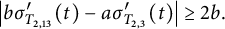 $$\begin{align*}\big | b\sigma^{\prime}_{T_{2,13}} (t) - a \sigma^{\prime}_{T_{2,3}}(t) \big| \ge 2b. \end{align*}$$
It follows that
 $\delta ([\mathcal {T}_{2,3}],[\mathcal {T}_{2,13}]) \ge 2$
. A construction such as in Section 2 shows that
$\delta ([\mathcal {T}_{2,3}],[\mathcal {T}_{2,13}]) \ge 2$
. A construction such as in Section 2 shows that
 $g_4( T_{2,13} \mathbin {\#} -4T_{2,3}) \le 2$
.
$g_4( T_{2,13} \mathbin {\#} -4T_{2,3}) \le 2$
.
The proof of Theorem 3.8 relied on the signature function, so we have the following corollary of Theorem 7.2.
Corollary 7.5 For any fixed integer
 $k \ge 1$
,
$k \ge 1$
,
 $$\begin{align*}\lim_{n \to \infty} \frac{\delta([\mathcal{T}_{2,2k+1}],[\mathcal{T}_{2, 2n+1}]) }{n} = \frac{1}{2k+1}. \end{align*}$$
7.1 Failure of the triangle inequality for
$\delta $
.

The results of Section 3.5 gave us the following.
-
•
$\delta (\{[\mathcal {T}_{2,41} ], [\mathcal {T}_{2,61}]) = 2$
. -
•
$\delta ([\mathcal {T}_{2,61}] ,[ \mathcal {T}_{2,91}]) = 2$
. -
•
$\delta ([\mathcal {T}_{2,41}] ,[ \mathcal {T}_{2,91}]) = 5$
.


To expand on this, applying Theorem 6.2, we have
-
•
$\Delta ([\mathcal {T}_{2,41} ], [\mathcal {T}_{2,61}]) = 2$
. -
•
$\Delta ([\mathcal {T}_{2,61}] , [\mathcal {T}_{2,91}]) = 2$
. -
•
$\Delta ([\mathcal {T}_{2,41}] ,[ \mathcal {T}_{2,91}])\le 4$
.


With this, the necessity of considering chains when defining
 $\Delta $
is apparent.
$\Delta $
is apparent.
8 The metric
$\Delta $
on
${\mathbb P}(\mathcal {C})$
and balls of small radius


Informally, Definition 6.1 states that the distance
 $\Delta ([\mathcal {K}],[ \mathcal {J}])$
is the minimal length of a path from
$\Delta ([\mathcal {K}],[ \mathcal {J}])$
is the minimal length of a path from
 $\mathcal {K}$
to
$\mathcal {K}$
to
 $\mathcal {J}$
formed from classes
$\mathcal {J}$
formed from classes
 $\mathcal {K}_i$
, where the length of each step is given by
$\mathcal {K}_i$
, where the length of each step is given by
 $\delta ([\mathcal {K}_i],[\mathcal {K}_{i+1}])$
. Theorem 6.3 states that the minimum can be realized by paths in which each step is of length 1. Thus, to understand the metric
$\delta ([\mathcal {K}_i],[\mathcal {K}_{i+1}])$
. Theorem 6.3 states that the minimum can be realized by paths in which each step is of length 1. Thus, to understand the metric
 $\Delta $
, it is important to understand balls for
$\Delta $
, it is important to understand balls for
 $\Delta $
-radius 1. In this section, we discuss this in the case of 2-stranded torus knots. We also include Theorem 8.4, stating a simple case in which a ball of radius 2 can be determined.
$\Delta $
-radius 1. In this section, we discuss this in the case of 2-stranded torus knots. We also include Theorem 8.4, stating a simple case in which a ball of radius 2 can be determined.
Our main application of the results of this section are presented as a series of examples in Section 9. The main goal of these examples is to emphasize the following: even if one is interested only in the restriction of the metric
 $\Delta $
to the projective space associated with a linear subspace of
$\Delta $
to the projective space associated with a linear subspace of
 $\mathcal {C}$
, in order to use such geometric results as Theorem 6.3, one must work in the full projective space
$\mathcal {C}$
, in order to use such geometric results as Theorem 6.3, one must work in the full projective space
 ${\mathbb P}(\mathcal {C})$
.
${\mathbb P}(\mathcal {C})$
.
8.1 Balls of radius one
In this subsection, we answer the question of determining all pairs of 2-stranded torus knots,
 $\mathcal {T}_1$
and
$\mathcal {T}_1$
and
 $\mathcal {T}_2$
, for which
$\mathcal {T}_2$
, for which
 $\delta ([\mathcal {T}_1],[\mathcal {T}_2]) = 1$
.
$\delta ([\mathcal {T}_1],[\mathcal {T}_2]) = 1$
.
Theorem 8.1 If
 $n>k$
and
$n>k$
and
 $\delta ([\mathcal {T}_{2,2k+1}], [\mathcal {T}_{2,2n+1}]) = 1$
, then either (1)
$\delta ([\mathcal {T}_{2,2k+1}], [\mathcal {T}_{2,2n+1}]) = 1$
, then either (1)
 $n = k+1, 2k +1$
, or
$n = k+1, 2k +1$
, or
 $3k+1$
, in which case the minimum is realized by
$3k+1$
, in which case the minimum is realized by
 $T_{2,2n+1} - \alpha T_{2k+1}$
, or (2)
$T_{2,2n+1} - \alpha T_{2k+1}$
, or (2)
 $n = 2k$
, in which case the minimum is realized by
$n = 2k$
, in which case the minimum is realized by
 $T_{2,2n+1} - (\alpha +1) T_{2, 2k+1}$
.
$T_{2,2n+1} - (\alpha +1) T_{2, 2k+1}$
.
Proof If
 $\delta ( [ \mathcal {T}_{2,2k+1}], [\mathcal {T}_{2,2n+1}] ) = 1$
, then for some a and b,
$\delta ( [ \mathcal {T}_{2,2k+1}], [\mathcal {T}_{2,2n+1}] ) = 1$
, then for some a and b,
 $g_4 ( bT_{2,2n+1}\mathbin {\#} - aT_{2,2k+1}) = 1$
. The signature condition implies that
$g_4 ( bT_{2,2n+1}\mathbin {\#} - aT_{2,2k+1}) = 1$
. The signature condition implies that
 $a=1$
and we are in the setting of Theorem 3.5.
$a=1$
and we are in the setting of Theorem 3.5.
The genus 1 surface is built as illustrated in Figures 1 and 2. In those diagrams, many of the bands have surgery curves going over them. Let the number of bands on the upper set that do not interact with surgery curves be denoted U. Let the lower count be L. In Figure 1, we have
 $U = 1 + 3 = 4$
and
$U = 1 + 3 = 4$
and
 $L=0$
. In Figure 2, we have
$L=0$
. In Figure 2, we have
 $U = 2$
and
$U = 2$
and
 $L=2$
. An important observation is that after surgery, the genus of the surface that results is
$L=2$
. An important observation is that after surgery, the genus of the surface that results is
 $(U+L)/2$
.
$(U+L)/2$
.
By Theorem 3.5, we need to consider two cases:
 $ T_{2,2n+1} \mathbin {\#} - \alpha T_{2,2k+1} $
and
$ T_{2,2n+1} \mathbin {\#} - \alpha T_{2,2k+1} $
and
 $ T_{2,2n+1} \mathbin {\#} - (\alpha -1) T_{2,2k+1} $
(recall that
$ T_{2,2n+1} \mathbin {\#} - (\alpha -1) T_{2,2k+1} $
(recall that
 $\alpha = \lfloor \frac {2n+1}{2k +1}\rfloor $
).
$\alpha = \lfloor \frac {2n+1}{2k +1}\rfloor $
).
Case 1:
 $ T_{2,2n+1}\mathbin {\#} - \alpha T_{2,2k+1} $
. (See Figure 1.) In this case, we have that
$ T_{2,2n+1}\mathbin {\#} - \alpha T_{2,2k+1} $
. (See Figure 1.) In this case, we have that
 $L=0$
and
$L=0$
and
 $U = (\alpha -1) +\big ( 2n - ( \alpha (2k+1) -1)\big ) $
, which simplifies to give
$U = (\alpha -1) +\big ( 2n - ( \alpha (2k+1) -1)\big ) $
, which simplifies to give
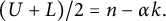 $$\begin{align*}(U + L)/2 = n - \alpha k.\end{align*}$$
If this equals 1, so that
 $n = \alpha k +1$
, we find
$n = \alpha k +1$
, we find
 $$\begin{align*}\alpha = \Big \lfloor \frac{2n+1}{2k+1}\Big \rfloor = \Big \lfloor \frac{2\alpha k +2+1}{2k+1}\Big \rfloor = \Big \lfloor \frac{2\alpha k + \alpha +3 - \alpha}{2k+1}\Big \rfloor = \Big \lfloor \alpha + \frac{ 3 - \alpha}{2k+1}\Big \rfloor. \end{align*}$$
Since
 $\alpha $
is a positive integer, this can occur only if
$\alpha $
is a positive integer, this can occur only if
 $1 \le \alpha \le 3$
.
$1 \le \alpha \le 3$
.
Case 2:
 $ T_{2,2n+1} \mathbin {\#} - (\alpha +1) T_{2,2k+1} $
. (See Figure 2.) In this case,
$ T_{2,2n+1} \mathbin {\#} - (\alpha +1) T_{2,2k+1} $
. (See Figure 2.) In this case,
 $U = \alpha $
. For the lower surface, we have
$U = \alpha $
. For the lower surface, we have
 $L = 2k - \big ( 2n - \alpha (2k+1) \big ) = 2k(\alpha +1) + \alpha -2n.$
Thus, we have
$L = 2k - \big ( 2n - \alpha (2k+1) \big ) = 2k(\alpha +1) + \alpha -2n.$
Thus, we have
 $$\begin{align*}(U + L) /2 = k\alpha + k +\alpha - n. \end{align*}$$
Thus, if this is 1, we have
 $n = k \alpha +k+\alpha -1$
, and
$n = k \alpha +k+\alpha -1$
, and
 $$\begin{align*}\alpha = \Big \lfloor \frac{2n+1}{2k+1}\Big \rfloor = \Big \lfloor \frac{2\alpha k +2k + 2\alpha - 2 +1 }{2k+1}\Big \rfloor = \Big \lfloor \frac{2\alpha k + \alpha +2k + \alpha - 1 }{2k+1}\Big \rfloor = \Big \lfloor \alpha + \frac{ 2k + \alpha - 1 }{2k+1}\Big \rfloor. \end{align*}$$
This is possible only if
 $$\begin{align*}\frac{ 2k + \alpha - 1 }{2k+1} < 1. \end{align*}$$
This implies that
 $\alpha < 2$
, that is,
$\alpha < 2$
, that is,
 $\alpha =1$
. This reduces to the case of
$\alpha =1$
. This reduces to the case of
 $n = 2k$
, as desired.
$n = 2k$
, as desired.
In the following corollary, we make a small change in notation, working with torus knots
 $T_{2,N}$
rather than
$T_{2,N}$
rather than
 $T_{2,2k+1}$
.
$T_{2,2k+1}$
.
Corollary 8.2 The ball of radius one about the class
 $[\mathcal {T}_{2,N}]$
contains the following classes:
$[\mathcal {T}_{2,N}]$
contains the following classes:
 $[\mathcal {T}_{2,N+2 }]$
,
$[\mathcal {T}_{2,N+2 }]$
,
 $[\mathcal {T}_{2,2N-1 }]$
,
$[\mathcal {T}_{2,2N-1 }]$
,
 $[\mathcal {T}_{2,2N+1 }]$
, and
$[\mathcal {T}_{2,2N+1 }]$
, and
 $[\mathcal {T}_{2,3N }]$
, and no other elements
$[\mathcal {T}_{2,3N }]$
, and no other elements
 $[\mathcal {T}_{2,N'}]$
with
$[\mathcal {T}_{2,N'}]$
with
 $N'> N$
.
$N'> N$
.
Example 8.3 The ball of radius one around the class
 $[\mathcal {T}_{2,15}]$
consists of the following set:
$[\mathcal {T}_{2,15}]$
consists of the following set:
 $$\begin{align*}B_1[(\mathcal{T}_{2,15}]) = \{[ \mathcal{T}_{2,5}], [\mathcal{T}_{2,7}],[ \mathcal{T}_{2,29}],[ \mathcal{T}_{2,31}], [\mathcal{T}_{2,45}]\}. \end{align*}$$
8.2 Balls of radius two
The following result will be used in Example 9.1, below.
Theorem 8.4 For
 $n = 5k+2$
,
$n = 5k+2$
,
 $\Delta ([\mathcal {T}_{2,2k+1}], [\mathcal {T}_{2,2n+1}]) = 2$
.
$\Delta ([\mathcal {T}_{2,2k+1}], [\mathcal {T}_{2,2n+1}]) = 2$
.
Proof A construction such as illustrated in Figure 1 shows that in the case that
 $n = 5k +2$
,
$n = 5k +2$
,
 $\delta ([\mathcal {T}_{2,2k+1}],[ \mathcal {T}_{2,2n+1}]) \le 2$
. The signature function, evaluated at
$\delta ([\mathcal {T}_{2,2k+1}],[ \mathcal {T}_{2,2n+1}]) \le 2$
. The signature function, evaluated at
 $\frac {3}{10k + 5} + \epsilon $
, can be used to show that this is an equality.
$\frac {3}{10k + 5} + \epsilon $
, can be used to show that this is an equality.
9 Linear spans
Given any subgroup
 $\mathcal {S} \subset \mathcal {C}$
, there is the projective space
$\mathcal {S} \subset \mathcal {C}$
, there is the projective space
 ${\mathbb P}(\mathcal {S})$
along with the metric
${\mathbb P}(\mathcal {S})$
along with the metric
 $\Delta _{\mathcal {S}}$
. In this section, we present a few examples, culminating with a demonstration that the inclusion
$\Delta _{\mathcal {S}}$
. In this section, we present a few examples, culminating with a demonstration that the inclusion
 $({\mathbb P}(\mathcal {S}), \Delta _s) \to ({\mathbb P}(\mathcal {C}), \Delta )$
need not be an isometry.
$({\mathbb P}(\mathcal {S}), \Delta _s) \to ({\mathbb P}(\mathcal {C}), \Delta )$
need not be an isometry.
Example 9.1 According to Theorem 8.4, we have that
 $\Delta (\mathcal {T}_{2,3}, \mathcal {T}_{2,15}) = 2$
. Notice that there is a chain:
$\Delta (\mathcal {T}_{2,3}, \mathcal {T}_{2,15}) = 2$
. Notice that there is a chain:
 $\delta (\mathcal {T}_{2,3}, \mathcal {T}_{2,5}) = 1$
and
$\delta (\mathcal {T}_{2,3}, \mathcal {T}_{2,5}) = 1$
and
 $\delta (\mathcal {T}_{2,5}, \mathcal {T}_{2,15}) = 1$
. There is also the chain:
$\delta (\mathcal {T}_{2,5}, \mathcal {T}_{2,15}) = 1$
. There is also the chain:
 $\delta (\mathcal {T}_{2,3}, \mathcal {T}_{2,7}) = 1$
and
$\delta (\mathcal {T}_{2,3}, \mathcal {T}_{2,7}) = 1$
and
 $\delta (\mathcal {T}_{2,7}, \mathcal {T}_{2,15}) = 1$
.
$\delta (\mathcal {T}_{2,7}, \mathcal {T}_{2,15}) = 1$
.
Example 9.2 Again, by Theorem 8.4, we have that
 $\Delta (\mathcal {T}_{2,5}, \mathcal {T}_{2,25}) = 2$
. However, there is no chain of length two among two-stranded torus knot classes with both steps of length one. Starting with
$\Delta (\mathcal {T}_{2,5}, \mathcal {T}_{2,25}) = 2$
. However, there is no chain of length two among two-stranded torus knot classes with both steps of length one. Starting with
 $\mathcal {T}_{2,5}$
, the results of the previous section show that the only knots within a
$\mathcal {T}_{2,5}$
, the results of the previous section show that the only knots within a
 $\delta $
-distance of 1 are
$\delta $
-distance of 1 are
 $\mathcal {T}_{2,3}, \mathcal {T}_{2,7}$
,
$\mathcal {T}_{2,3}, \mathcal {T}_{2,7}$
,
 $\mathcal {T}_{2,9}$
,
$\mathcal {T}_{2,9}$
,
 $\mathcal {T}_{2,11}$
, and
$\mathcal {T}_{2,11}$
, and
 $\mathcal {T}_{2,15}$
. The radius one balls around these include
$\mathcal {T}_{2,15}$
. The radius one balls around these include
 $ \mathcal {T}_{2,9 }$
,
$ \mathcal {T}_{2,9 }$
,
 $ \mathcal {T}_{2,13 }$
,
$ \mathcal {T}_{2,13 }$
,
 $ \mathcal {T}_{2,15 }$
,
$ \mathcal {T}_{2,15 }$
,
 $ \mathcal {T}_{2,21 }$
,
$ \mathcal {T}_{2,21 }$
,
 $ \mathcal {T}_{2,11 }$
,
$ \mathcal {T}_{2,11 }$
,
 $ \mathcal {T}_{2,17 }$
,
$ \mathcal {T}_{2,17 }$
,
 $ \mathcal {T}_{2,19 }$
,
$ \mathcal {T}_{2,19 }$
,
 $ \mathcal {T}_{2,27 }$
,
$ \mathcal {T}_{2,27 }$
,
 $ \mathcal {T}_{2,17 }$
,
$ \mathcal {T}_{2,17 }$
,
 $ \mathcal {T}_{2,29 }$
,
$ \mathcal {T}_{2,29 }$
,
 $ \mathcal {T}_{2,31 }$
, and
$ \mathcal {T}_{2,31 }$
, and
 $ \mathcal {T}_ {2,45 }$
. Notice that
$ \mathcal {T}_ {2,45 }$
. Notice that
 $\mathcal {T}_{2, 25} $
is not on the list.
$\mathcal {T}_{2, 25} $
is not on the list.
Theorem 6.3 implies that there is a knot
 $\mathcal {J}$
for which
$\mathcal {J}$
for which
 $\delta (\mathcal {T}_{2,5}, \mathcal {J}) = 1$
and
$\delta (\mathcal {T}_{2,5}, \mathcal {J}) = 1$
and
 $\delta (\mathcal {J}, \mathcal {T}_{2,25}) =1$
. One example is
$\delta (\mathcal {J}, \mathcal {T}_{2,25}) =1$
. One example is
 $\mathcal {J} = 2\mathcal {T}_{2,5} \mathbin {\#} \mathcal {T}_{2,15}$
. We leave it as an exercise to find a pair of band moves that converts
$\mathcal {J} = 2\mathcal {T}_{2,5} \mathbin {\#} \mathcal {T}_{2,15}$
. We leave it as an exercise to find a pair of band moves that converts
 $5\mathcal {T}_{2,5}$
into
$5\mathcal {T}_{2,5}$
into
 $\mathcal {J}$
, and another pair of band moves that converts
$\mathcal {J}$
, and another pair of band moves that converts
 $\mathcal {J}$
into
$\mathcal {J}$
into
 $\mathcal {T}_{2,25}$
.
$\mathcal {T}_{2,25}$
.
Example 9.3 Continuing with the example of the pair
 $\mathcal {T}_{2,5}$
and
$\mathcal {T}_{2,5}$
and
 $\mathcal {T}_{2,25} $
, a simple calculation shows that if
$\mathcal {T}_{2,25} $
, a simple calculation shows that if
 $K = aT_{2,5} \mathbin {\#} cT_{2,25} $
and
$K = aT_{2,5} \mathbin {\#} cT_{2,25} $
and
 $\epsilon $
is small, then
$\epsilon $
is small, then
 $\big | \sigma ^{\prime }_K(\frac {1}{5} - \epsilon )\big | = \big | 2c\big |$
. It follows that the unit
$\big | \sigma ^{\prime }_K(\frac {1}{5} - \epsilon )\big | = \big | 2c\big |$
. It follows that the unit
 $\delta $
-ball around the element
$\delta $
-ball around the element
 $[\mathcal {T}_{2,5}]$
within the projective space of the two-dimensional span
$[\mathcal {T}_{2,5}]$
within the projective space of the two-dimensional span
 $\left < \mathcal {T}_{2,5}, \mathcal {T}_{2,25}\right>$
is the single element
$\left < \mathcal {T}_{2,5}, \mathcal {T}_{2,25}\right>$
is the single element
 $[\mathcal {T}_{2,5}]$
. In particular, although Theorem 6.3 guarantees the existence of two step paths joining thee classes, the only such paths must leave the projective space of the span of these two knots.
$[\mathcal {T}_{2,5}]$
. In particular, although Theorem 6.3 guarantees the existence of two step paths joining thee classes, the only such paths must leave the projective space of the span of these two knots.
Example 9.4 Let
 $\mathcal {S} = \left < \mathcal {T}_{2,41} , \mathcal {T}_{2,91}\right>$
. The inclusion
$\mathcal {S} = \left < \mathcal {T}_{2,41} , \mathcal {T}_{2,91}\right>$
. The inclusion
 ${\mathbb P}(\mathcal {S} ) \to {\mathbb P}(\mathcal {C})$
is not an isometry. From Section 3.5, we have that the distance between any two elements in
${\mathbb P}(\mathcal {S} ) \to {\mathbb P}(\mathcal {C})$
is not an isometry. From Section 3.5, we have that the distance between any two elements in
 $\mathcal {S}$
is at least 5, so that the projective distance
$\mathcal {S}$
is at least 5, so that the projective distance
 $\Delta _{\mathcal {S}}([\mathcal {T}_{2,41}] ,[ \mathcal {T}_{2,91}])\ge 5$
. In fact, the distance is precisely 5. On the other hand, we saw in that section that in
$\Delta _{\mathcal {S}}([\mathcal {T}_{2,41}] ,[ \mathcal {T}_{2,91}])\ge 5$
. In fact, the distance is precisely 5. On the other hand, we saw in that section that in
 ${\mathbb P}(\mathcal {C})$
we have
${\mathbb P}(\mathcal {C})$
we have
 ${\Delta ([\mathcal {T}_{2,41}] , [\mathcal {T}_{2,91}]) \le 4}$
.
${\Delta ([\mathcal {T}_{2,41}] , [\mathcal {T}_{2,91}]) \le 4}$
.
10 A simplical complex built from
${\mathbb P}(\mathcal {C})$

There is a canonical simplicial complex associated with
 $({\mathbb P}(\mathcal {C}), \Delta )$
, denoted
$({\mathbb P}(\mathcal {C}), \Delta )$
, denoted
 $\overline {({\mathbb P}(\mathcal {C}), \Delta )}$
, which we will abbreviate
$\overline {({\mathbb P}(\mathcal {C}), \Delta )}$
, which we will abbreviate
 $\overline {{\mathbb P}(\mathcal {C})}$
. We introduce it here to provide concise statements of basic questions about the metric properties of
$\overline {{\mathbb P}(\mathcal {C})}$
. We introduce it here to provide concise statements of basic questions about the metric properties of
 $ P(\mathcal {C})$
.
$ P(\mathcal {C})$
.
For any set with integer-valued metric,
 $(X, d)$
, there is an embedding of X into a simplicial complex
$(X, d)$
, there is an embedding of X into a simplicial complex
 $\overline {(X,d)}$
. By definition, an n-simplex of
$\overline {(X,d)}$
. By definition, an n-simplex of
 $\overline {(X,d)}$
consists of a set of distinct elements
$\overline {(X,d)}$
consists of a set of distinct elements
 $\{x_0, \ldots , x_n\}$
such that
$\{x_0, \ldots , x_n\}$
such that
 $d(x_i, x_j) = 1$
if
$d(x_i, x_j) = 1$
if
 $i\ne j$
. This is an example of a Vietoris–Rips complex [Reference Hausmann10].
$i\ne j$
. This is an example of a Vietoris–Rips complex [Reference Hausmann10].
Example 10.1 The following is a
 $3$
-simplex of
$3$
-simplex of
 $\overline {{\mathbb P}(\mathcal {C})}$
:
$\overline {{\mathbb P}(\mathcal {C})}$
:
 $\{ [\mathcal {T}_{2,3}], [\mathcal {T}_{2,5}] , [\mathcal {T}_{2,7}] , [\mathcal {T}_{2,3} \mathbin {\#} \mathcal {T}_{2,5}] \}$
.
$\{ [\mathcal {T}_{2,3}], [\mathcal {T}_{2,5}] , [\mathcal {T}_{2,7}] , [\mathcal {T}_{2,3} \mathbin {\#} \mathcal {T}_{2,5}] \}$
.
Example 10.2 There exists an infinite set of n-simplices in
 $\overline {{\mathbb P}(\mathcal {C})}$
. Let
$\overline {{\mathbb P}(\mathcal {C})}$
. Let
 $K_n$
be the n-twisted double of the unknot with clasp chosen so that the Seifert form is
$K_n$
be the n-twisted double of the unknot with clasp chosen so that the Seifert form is
 $ \begin {pmatrix} 1 & 1 \\ 0 & n \\ \end {pmatrix}.$
The set
$ \begin {pmatrix} 1 & 1 \\ 0 & n \\ \end {pmatrix}.$
The set
 $\{K_n\}_{n \ge 1}$
is linearly independent; this follows from the independence of the signature functions, which have jumps at complex numbers
$\{K_n\}_{n \ge 1}$
is linearly independent; this follows from the independence of the signature functions, which have jumps at complex numbers
 $e^{\theta _n i} $
where
$e^{\theta _n i} $
where
 $\cos (\theta _n) = 1 - \frac {1}{2n}$
. (These knots were first used to show that
$\cos (\theta _n) = 1 - \frac {1}{2n}$
. (These knots were first used to show that
 $\mathcal {C}$
contains an infinite free summand by Milnor [Reference Milnor18].)
$\mathcal {C}$
contains an infinite free summand by Milnor [Reference Milnor18].)
The knot
 $K_n$
can be unknotted with a single negative to positive crossing change. Thus,
$K_n$
can be unknotted with a single negative to positive crossing change. Thus,
 $K_n \mathbin {\#} -K_m$
can by unknotted with one positive and one negative crossing change. It follows that
$K_n \mathbin {\#} -K_m$
can by unknotted with one positive and one negative crossing change. It follows that
 $K_n \mathbin {\#} -K_m$
bounds a disk in
$K_n \mathbin {\#} -K_m$
bounds a disk in
 $B^4$
with two double points of opposite sign. A simple tubing construction yields an embedded punctured torus, showing that
$B^4$
with two double points of opposite sign. A simple tubing construction yields an embedded punctured torus, showing that
 $\Delta ( [\mathcal {K}_n], [\mathcal {K}_m]) = 1$
. Thus, any set of
$\Delta ( [\mathcal {K}_n], [\mathcal {K}_m]) = 1$
. Thus, any set of
 $n+1$
of these knots yields an n-simplex in
$n+1$
of these knots yields an n-simplex in
 $\overline {{\mathbb P}(\mathcal {C})}$
.
$\overline {{\mathbb P}(\mathcal {C})}$
.
Example 10.3 There exists an infinite set of n-simplices in
 $\overline {{\mathbb P}(\mathcal {C})}$
spanned by algebraically slice knots. We work with the same knots
$\overline {{\mathbb P}(\mathcal {C})}$
spanned by algebraically slice knots. We work with the same knots
 $K_n$
but use the set of knots
$K_n$
but use the set of knots
 $\{ K_n \}$
where n is restricted to be of the form
$\{ K_n \}$
where n is restricted to be of the form
 $n= -k(k+1)$
for some
$n= -k(k+1)$
for some
 $k\ge 2$
. Using the results of [Reference Casson and Gordon3], Jiang [Reference Jiang14] proved that the concordance classes of these knots are linearly independent over
$k\ge 2$
. Using the results of [Reference Casson and Gordon3], Jiang [Reference Jiang14] proved that the concordance classes of these knots are linearly independent over
 ${\mathbb Z}$
. The same proof as in the previous example shows that they are all of
${\mathbb Z}$
. The same proof as in the previous example shows that they are all of
 $\Delta $
-distance 1 from each other.
$\Delta $
-distance 1 from each other.
11 Problems
Here are a few problems.
-
(1) Show that
$({\mathbb P}(\mathcal {C}), \Delta )$
is unbounded. -
(2) Show that every element of
$({\mathbb P}(\mathcal {C}), \Delta )$
has infinite order; that is, the ball of radius one about every element is infinite. In [Reference Hirasawa and Uchida13], Hirasawa and Uchida proved such a statement for the Gordian complex of the set of knots, where distance is determined by the minimal number of crossing changes required to convert one knot into another; further results were obtained by Baader [Reference Baader1]. The invariants used in those papers do not seem to be applicable in working with
${\mathbb P}(\mathcal {C})$
. -
(3) Under what conditions on
$\mathcal {S}$
is the map
$({\mathbb P}(\mathcal {S}),\Delta _{\mathcal {S}}) \to ({\mathbb P}(\mathcal {C}), \Delta )$
isometric? Note that in Example 9.4 we saw that the inclusion
${\mathbb P}(\left < \mathcal {T}_{2,41}, \mathcal {T}_{2,91}\right> )\to {\mathbb P}(\mathcal {C})$
is not an isometry. One might conjecture that if
$\mathcal {S}$
is the span of positive (or strongly quasipositive) knots, then the inclusion is isometric. (The importance of strongly quasipositive knots appeared in the work of Rudolph [Reference Rudolph22] and has been extensively studied from the perspective of Heegaard Floer theory; see, for instance, [Reference Hedden11].) -
(4) A metric can be defined on
${\mathbb P} (\mathcal {C} / {\text {Torsion}} )$
by modifying Definition 6.1 so that the path is restricted to nontorsion classes. Using this metric, is the injection
${\mathbb P} (\mathcal {C} / {\text {Torsion}} ) \to {\mathbb P}(\mathcal {C})$
isometric? -
(5) Let
$\mathcal {S}$
denote the concordance group of topologically slice knots or the subgroup generated by knots with Alexander polynomial
$A_K(t) =1$
. What can be said about
$({\mathbb P}(\mathcal {S}), \Delta _{\mathcal {S}})$
? In particular, what is the dimension of
$\overline {({\mathbb P}(\mathcal {S}), \Delta )}$
? -
(6) Let d be a metric on
${\mathbb Z} \oplus {\mathbb Z}$
; for instance, one can build d using the
$L^1$
-norm
$\big | (a, b) \big | = \max \{ \big | a\big |, \big | b \big | \}$
. Describe the metric space
$({\mathbb P}({\mathbb Z} \oplus {\mathbb Z}), \Delta )$
. Notice that
${\mathbb P}({\mathbb Z} \oplus {\mathbb Z})$
is in natural bijective correspondence with the 1-dimensional rational projective line
${\mathbb Q}{\mathbb P}^1$
. What can be said about the simplicial complex
$\overline {{\mathbb P}({\mathbb Z} \oplus {\mathbb Z}), \Delta )}$
?Here are two simple examples that illustrate a property of
$ {{\mathbb P}({\mathbb Z} \oplus {\mathbb Z}), \Delta )}$
. The arrows indicate steps of length 1.
$$\begin{align*}(8,15) \to (8,14) \sim (4,7) \to (4,6) \sim (2,3) \to (2,2) \sim (1,1), \end{align*}$$
$$\begin{align*}(135, 173) \to (135, 174) \sim (45, 58) \to (44,58) \sim (22,29) \to \hskip.4in \end{align*}$$
$$\begin{align*}\hskip1.5in (21,28) \sim (3,4) \to (3,3) \sim (1,1). \end{align*}$$
The first example, showing that
$\Delta ( (8,15) ,(1,1)) \le 3$
, points to the fact that in general
$ \Delta ( (x,y) ,(1,1))$
is bounded above by something of the order of
$\max \{ \log _2(x), \log _2(y)\}$
. The second indicates that this bound is probably a significant overestimate in many cases.


Acknowledgment
I thank Samantha Allen for her valuable feedback on early drafts of the manuscript. Referees provided unusually thoughtful and detailed commentary that significantly improved the exposition of the paper.


