


1. Introduction
Particle transport in a porous medium is important for a broad range of applications in biomedical, chemical, environmental and geotechnical engineering. For instance, transport of microplastic particles in soil is a problem of growing significance due the effect of these particles on soil biota, such as earthworms, and their further propagation up the food chain (Chu et al. Reference Chu, Li, Yan and Shen2019; Fu et al. Reference Fu, Min, Jiang, Li and Zhang2020; Waldschläger et al. Reference Waldschläger, Lechthaler, Stauch and Schüttrumpf2020). Transport and dispersion of proppant particles through cracks and crevices in fractured rock during hydraulic fracturing operations is a key step in oil recovery from shale, acting to significantly increase a reservoir's permeability to oil and gas transport (Deng et al. Reference Deng, Li, Ma, Huang and Li2014; Liang et al. Reference Liang, Sayed, Al-Muntasheri, Chang and Li2016). Nanoparticles are commonly used in biofilm mitigation processes, either due to the direct interaction between the bacteria and certain metals (e.g. silver), for thermal ablation of the biofilm or as carriers of antimicrobial substances into the biofilm (Peulen & Wilkinson Reference Peulen and Wilkinson2011; Forier et al. Reference Forier, Raemdonck, De Smedt, Demeester, Coenye and Braeckmans2014; Millenbaugh et al. Reference Millenbaugh, Baskin, DeSilva, Elliot and Glickman2015; Han et al. Reference Han, Romero, Fischer, Dookran, Berger and Doiron2017; Li et al. Reference Li, Nickel, Wu, Lin, van Lierop and Liu2019; Siddique et al. Reference Siddique2020). The nanoparticles are transported through the porous biofilm extracellular polymeric substance layer either by diffusion or under the driving effect of an external field, such as a magnetic field or ultrasound (Ma et al. Reference Ma, Green, Willsey, Marshall, Wargo and Wu2015; Quan et al. Reference Quan, Zhang, Ren, Busscher, van der Mei and Peterson2020). In a similar application, nanoparticles are widely used as carriers in targeted drug delivery to diseased tissues (Bahrami et al. Reference Bahrami, Hojjat-Farsangi, Mohammadi, Anvari, Ghalamfarsa, Yousefi and Jadidi-Niaragh2017; Patra et al. Reference Patra2018; Mitchell et al. Reference Mitchell, Billingsley, Haley, Wechsler, Peppas and Langer2021). Targeted drug delivery can be highly effective for overcoming drug resistance problems and it helps chemotherapy drugs to be more directly targeted at diseased tissue and to have less of a negative impact on healthy tissue (Yao et al. Reference Yao, Zhou, Liu, Xu, Chen, Wang, Wu, Deng, Zhang and Shao2020).
Traditional continuum models for particle transport in a porous medium solve a one-dimensional convection–diffusion equation with two important modifications: (1) the diffusion coefficient is modified to account for the sum of molecular diffusion and particle dispersion, where the last term is proportional to the nominal velocity of particles within the bed, and (2) a particle sink term is included representing capture of particles by the porous medium (Benamar et al. Reference Benamar, Ahfir, Wang and Alem2007; Chen, Zhang & Wu Reference Chen, Zhang and Wu2019). The parameters used in continuum models (diffusion coefficient, capture rate coefficient, etc.) must be estimated from experimental data for a specific problem, and cannot generally be determined a priori from the physical characteristics of the porous medium and particles (Babakhani et al. Reference Babakhani, Bridge, Doong and Phenrat2017). Continuum models utilize many simplifying assumptions, which may not be consistent with the mechanisms for particle capture and detachment or particle diffusion/dispersion for a given problem, and are particularly sensitive to changes in problem scaling.
Particle capture, and possible later particle detachment, is a key characteristic of colloidal particle transport in porous media (McDowell-Boyer, Hunt & Sitar Reference McDowell-Boyer, Hunt and Sitar1986; Molnar et al. Reference Molnar, Johnson, Gerhard, Willson and O'Carroll2015). For dilute suspensions consisting of sufficiently small particles that are much smaller than the porous medium pore size, particle capture is dominated by adhesive forces (van der Waals, electrostatic), as represented in the Derjaguin–Landau–Verwey–Overbeek theory (Derjaguin & Landau Reference Derjaguin and Landau1941; Verwey & Overbeek Reference Verwey and Overbeek1948). More recent modifications have been proposed to improve predictive capability of this theory by accounting for surface roughness (Rasmuson et al. Reference Rasmuson, Pazmino, Assemi and Johnson2017; Shen et al. Reference Shen, Jin, Zhuang, Li and Xing2020) and hydrodynamic effects on particle impact (Torkzaban, Bradford & Walker Reference Torkzaban, Bradford and Walker2007; Shen et al. Reference Shen, Huang, Li and Jin2010). On the opposite end of the spectrum, for relatively large particles of size of the magnitude of the pore size, particle straining becomes the dominant mechanism controlling particle capture (McDowell-Boyer et al. Reference McDowell-Boyer, Hunt and Sitar1986; Bradford et al. Reference Bradford, Yates, Bettahar and Simunek2002, Reference Bradford, Simunek, Bettahar, van Genuchten and Yates2006). While for dilute particle suspensions straining depends primarily on the ratio of particle size to pore size, cases with higher particle concentrations or with a mixture of particles of different sizes can exhibit bridging and jamming effects that lead to straining capture even for cases with particles much smaller than the pore size (Porubcan & Xu Reference Porubcan and Xu2011). Bizmark et al. (Reference Bizmark, Schneider, Priestley and Datta2020) report a study in which motion of individual particles in a porous bed was directly visualized, illustrating the build-up of particle bridges leading to cake formation as the particle concentration increases.
Pore-scale modelling seeks to simulate the transport of individual particles within a porous medium, the results of which can be used to both motivate and validate models for specific terms in continuum models (Boccardo et al. Reference Boccardo, Tosco, Fujisaki, Messina, Raoof, Aguilera, Crevacore, Marchisio, Sethi, Bonelli, Frayria, Rossetti and Sethi2020). Particle transport modelling at the pore scale is advantageous compared with macroscopic methods for studying interactions between individual particles, the porous structure and the modelled fluid that affect particle retention mechanisms and transport processes at larger scales. Li, Yu & Fan (Reference Li, Yu and Fan2021) and Kermani et al. (Reference Kermani, Jafari, Rahnama and Raoof2020) present simulations of particle transport within a tube of variable diameter as a representation of the pore variation in a regularly structured porous medium (such as a bed of spheres arranged in simple cubic structure). Pore-scale simulations of fluid and particle transport within a two-dimensional network of channels representing fractures in a rock are reported by Su et al. (Reference Su, Chai, Wang, Cao, Gu, Chen and Xu2019), in which the discrete-element method (DEM) is used to simulate particle interactions. Zhou et al. (Reference Zhou, Chen, Gong and Wang2021) present simulations for a two-dimensional porous medium formed of a random array of circular beads in which the lattice Boltzmann method (LBM) for flow simulation is combined with a DEM for particle transport. The paper focuses on illustrating the mechanisms leading to particle deposition and clogging in the porous medium.
Elrahmani et al. (Reference Elrahmani, Al-Raoush, Abugazia and Seers2022) combined computational fluid dynamics to model fluid flow with the DEM for particle transport in heterogeneous porous media. They investigated the impact of fine particle sizes and flow velocity on permeability reduction of the porous media. Endo Kokubun et al. (Reference Endo Kokubun, Muntean, Radu, Kumar, Pop, Keilegavlen and Spildo2019) presented simulations of inertial particle transport in a porous bed to illustrate particle accumulation and pore throat clogging due to hydrodynamic effects caused by the porous medium's geometry and fluid flow dynamics. Sadeghnejad et al. (Reference Sadeghnejad, Enzmann and Kersten2022) examined the particle retention mechanisms that affect pore structure permeability, varying particle size and velocity as well as surface roughness and adhesion forces. The paper showed that clogging is responsible for permeability reduction when particle size and adhesion forces are increased, but not when surface roughness is increased. Sanematsu, Thompson & Willson (Reference Sanematsu, Thompson and Willson2019) also studied the effects of varying attractive surface force strengths on particle deposition in a realistic material, using a three-dimensional model generated from X-ray microtomography images of Berea sandstone samples. Realistic pore geometries allowed researchers to model particle transport processes directly on structures taken from real materials, though this approach requires intricate image analysis techniques and discretization algorithms for simulation. More commonly, porous materials are modelled with simplified structures, typically using synthetic sphere packs to represent solid grains and generate the porous domain. Randomly packed spherical particles are often used to maintain a realistic modelling experience, such as in the granular filter study presented by Abelhamid & El Shamy (Reference Abelhamid and El Shamy2016). Organized beds of spheres are also commonly utilized, with porous bed particles being arranged in arrays like a face-centred cubic structured pack for which the porosity is well known (Apte et al. Reference Apte, Oujia, Matsuda, Kadoch, He and Schneider2022).
Despite recent progress, existing pore-scale models for particle transport in porous media have not clarified the mechanisms governing particle lateral drift in the flow channels, understanding of which is critical in order to accurately model particle collision with the fixed bed particles and resulting adhesive hold-up of colloidal particles (Narayan et al. Reference Narayan, Coury, Masliyah and Gray1997). Using pore-scale simulations of particle transport in a three-dimensional porous bed, the current paper examines the role of oscillatory clustering (Marshall Reference Marshall2009b; Hewitt & Marshall Reference Hewitt and Marshall2010) in the lateral particle transport within flow channels, as well as the effect of particle collision with the fixed bed and subsequent van der Waals adhesion on inhibiting particle lateral transport. The numerical simulations use fixed spherical beads in a body-centred cubic (BCC) structure, which was selected in order to provide tortuosity of the particle path typical of flow in a packed bed (e.g. Kampel, Goldsztein & Santamarina Reference Kampel, Goldsztein and Santamarina2009) while at the same time simplifying the computations by forming a regular periodic structure. In order to focus on particle lateral drift and avoid obscuring effects of other particles, the reported particle transport simulations each used a single moving particle with one-way fluid particle coupling. Each computation was repeated 400 times with different initial conditions to obtain statistics for particle transport through the porous bed in the absence of other particles.
The simulation of the fluid flow through the bed is described in § 2, and the adhesive DEM used for particle transport through the bed is described in § 3. Computational results with non-adhesive particles are reported in § 4, which quantify the straining and velocity fields experienced by particles passing through the packed bed and the resulting lateral displacement, as well as various measures describing particle collision with the bed spheres. Section 5 examines the role of adhesive forces acting between the movable particles and bed spheres in the various measures characterizing the particle dynamics. Key dimensionless parameters examined include the ratio of particle diameter to average pore size and the particle Stokes and adhesion numbers. Conclusions are given in § 6.
2. Fluid flow simulation
2.1. Governing equations
The fluid flow is governed by the steady-state incompressible continuity and Navier–Stokes equations in three dimensions, given by
 \begin{gather}\boldsymbol{\nabla }\boldsymbol{\cdot }\boldsymbol{u} = 0,\end{gather}
 \begin{gather}\rho (\boldsymbol{u}\boldsymbol{\cdot }\boldsymbol{\nabla })\boldsymbol{u} = \rho \boldsymbol{g} - \boldsymbol{\nabla }p + \mu {\nabla ^2}\boldsymbol{u}.\end{gather}
In these equations, u,  $\rho $ and
  $\mu $ are the fluid velocity, density and viscosity, respectively, p is pressure and g is an imposed body force used to generate the flow.
The paper examines fluid flow through a porous bed formed of fixed spherical particles, driven by a body force acting on the fluid in the x direction of a Cartesian coordinate system (x, y, z). The arrangement of the fixed bed particles was based on the BCC structure with BCC cell side length L. Each BCC unit cell contains one particle at the cell centre and eight one-eighth particle sections in the cell corners. The resulting particle coordination number is eight, and the bed porosity is  $\phi = 0.32$. The computational domain extended two BCC cells wide in each of the cross-sectional y and z directions, and five BCC cells long in the x direction (figure 1). Periodic boundary conditions were applied to each side of the domain surrounding the porous bed. The periodic boundaries of the fluid domain were located such as to bisect the fixed particles along the edge of the domain to provide a periodic geometric structure for bed particles.

Figure 1. Computational domain used to calculate fluid velocity field through porous bed of particles in (a) the y–z plane and (b) the x–y plane.
2.2. Numerical simulations
The fluid flow was computed using the LBM, and the no-slip condition was applied at the surface of the fixed bed particles with use of the immersed boundary method (IBM). Details of the LBM–IBM computational method used for the fluid flow are given in Appendix A.
A nominal velocity was computed for each flow case examined using the ratio  ${u_{nom}} = Q/{A_C}$, where Q is the volumetric flow rate over the computational domain cross-section with area
  ${A_C} = 4{L^2}$. This quantity is also called the discharge rate or the discharge flux in some porous flow literature. The flow variables were non-dimensionalized using the cubic BCC cell side length L as a length scale and the nominal velocity
  $U = {u_{nom}}$ as a velocity scale. Time was non-dimensionalized using the corresponding convection time scale
  $L/U$. Variables non-dimensionalized using this scaling are indicated with a prime. A Reynolds number
  $Re = {u_{nom}}L/\nu $ was defined based on the nominal velocity and the BCC cell side length. Computations are examined in the paper for Reynolds numbers of Re = 0.02, 0.5 and 8. Using this non-dimensionalization, the fixed bed particles have uniform diameter
  ${d^{\prime}_b} = \sqrt 3 /2 \cong 0.866$. The characteristic pore size in the BCC array can be set equal to the gap width between neighbouring particles in a given cross-sectional plane, or
  $\delta ^{\prime} = 1 - \sqrt 3 /2 \cong 0.134$. This distance is the same as the diameter of the largest sphere that can be circumscribed in the gap between three touching spherical particles of diameter
  ${d^{\prime}_b}$.
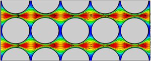
An example showing the simulated flow field is given in figure 2 for a case with  $Re = 0.5$. Images are shown both for a perspective view of the x velocity component on the computational domain boundary and for x velocity and streamlines on a slice in the x–z and x–y planes along the flow midplane. The flow is observed to primarily occur in a set of channels within the BCC array, where from figure 2(b) the channel appears to have a corrugated boundary, such that the cross-sectional area of the channel varies periodically with distance along the channel. The velocity field in a slice across the domain in the x–y plane appears very similar to the slice in the x–z plane, but the oscillations in the two planes are 90° out of phase (figure 2b). Consequently, the flow along each channel experiences two oscillations per BBC length – one oscillation in the z direction and one in the y direction.

Figure 2. Contours of the dimensionless velocity magnitude in the x direction and streamlines computed by the LBM for fluid flow through the porous bed with Re = 0.5, for (a) three-dimensional volume and (b) slice of the fluid flow in the x–z and x–y planes.
A grid independence study was performed using grid sizes with  ${N_{cell}} = 20$, 40, 60 and 80 points across each BCC cell. Grid increment sizes in all three directions were set to be the same, so that
  $\mathrm{\Delta }x = \mathrm{\Delta }y = \mathrm{\Delta }z$. A plot showing the dimensionless maximum pore velocity
  ${u^{\prime}_{max}}$ as a function of the total number of grid nodes is given in figure 3 for
  $Re = 0.5$. The figure demonstrates that the flow has achieved close to grid independence at
  ${N_{cell}} = 60$ (or slightly over 4 million grid nodes), which is used for the remainder of the computations.

Figure 3. Dimensionless maximum velocity in porous bed as a function of number of grid nodes for Re = 0.5.
Flow within the porous bed can be approximated using Darcy's law, which for gravitationally driven flow can be written as
 \begin{equation}{u_{nom}} =- \frac{\kappa }{\mu }\frac{{\partial p}}{{\partial x}} = \frac{{\kappa g}}{\nu },\end{equation}
where  $\kappa $ is the hydraulic permeability. From (2.3), we can solve for the dimensionless permeability
  ${\kappa _r} = \kappa /{d^2}$ to write
 \begin{equation}{\kappa _r} = \frac{{\nu {u_{nom}}}}{{{d^2}g}}.\end{equation}
Lattice Boltzmann simulations for flow past various periodic arrays of spheres were given by Hill, Koch & Ladd (Reference Hill, Koch and Ladd2001), Van der Hoef, Beetstra & Kuipers (Reference Van der Hoef, Beetstra and Kuipers2005), Maier et al. (Reference Maier, Kroll, Davis and Bernard1998) and Maier & Bernard (Reference Maier and Bernard2010). For the close-packed BCC array, expressions at low Reynolds numbers were summarized by Blazejewski & Murat-Blazejewski (Reference Blazejewski and Murat-Blazejewski2014) and experimental studies were reported by Franzen (Reference Franzen1979). Maier et al. (Reference Maier, Kroll, Davis and Bernard1998) reported that accurate values of dimensionless permeability for close-packed arrays at low Reynolds number are given by the Richardson–Zaki equation (Richardson & Zaki Reference Richardson and Zaki1954):
 \begin{equation}{\kappa _r} = \frac{{{\phi ^\alpha }}}{{18(1 - \phi )}},\end{equation}
with the exponent  $\alpha $ set equal to 5.0. Computed values of dimensionless permeability are compared with the experimental value from Franzen (Reference Franzen1979) and the Richardson–Zaki prediction in table 1 for the three different Reynolds numbers examined. The predicted result at low Re is about 20 % higher than the Franzen (Reference Franzen1979) experimental value and exactly the same as the Richardson–Zaki correlation prediction. The observation of decreasing permeability with increase in Re is also consistent with experimental data (e.g. Franzen Reference Franzen1979).
Table 1. Comparison of computed dimensionless permeability values from current paper at different Reynolds numbers and comparison values.

3. Particle transport simulation
3.1. Governing equations
Particle transport within the packed bed was simulated using an adhesive DEM with one-way fluid–particle coupling. The DEM algorithm transports individual particles by solution of the particle momentum and angular momentum equations:
 \begin{equation}m\frac{{\textrm{d}\boldsymbol{v}}}{{\textrm{d}t}} = {\boldsymbol{F}_F} + {\boldsymbol{F}_A},\quad I\frac{{\textrm{d}\boldsymbol{\varOmega }}}{{\textrm{d}t}} = {\boldsymbol{M}_F} + {\boldsymbol{M}_A},\end{equation}
subject to forces and torques induced by the fluid flow ( ${\boldsymbol{F}_F}$ and
  ${\boldsymbol{M}_F}$) and by the combined particle collision and adhesion (
 ${\boldsymbol{F}_A}$ and
  ${\boldsymbol{M}_A}$). Here, m is the particle mass, I is the moment of inertia and v and
  $\boldsymbol{\varOmega}$ are the particle velocity and rotation rate, respectively.
The dominant fluid force is the drag force, which is given by the Stokes drag law as
 \begin{equation}{\boldsymbol{F}_d} = 3{\rm \pi} \mu d(\boldsymbol{u} - \boldsymbol{v}),\end{equation}
where u is the fluid velocity evaluated at the particle centroid and d is the particle diameter. The associated viscous fluid torque arises from a difference in rotation rate of the particle and the local fluid element, and was given by Crowe et al. (Reference Crowe, Schwarzkopf, Sommerfeld and Tsuji2012) as
 \begin{equation}{\boldsymbol{M}_F} =- {\rm \pi}\mu {d^3}(\boldsymbol{\varOmega } - {\textstyle{1 \over 2}}\boldsymbol{\omega }),\end{equation}
where  $\boldsymbol{\omega }$ is the fluid vorticity vector at the particle centroid.
Other fluid forces included in the computation are the Saffman and Magnus lift terms (Rubinow & Keller Reference Rubinow and Keller1961; Saffman Reference Saffman1965, Reference Saffman1968) and the added mass and pressure gradient forces, which together with drag make up the total fluid force  ${\boldsymbol{F}_F}$. The added mass force
  ${\boldsymbol{F}_{a}}$ and the pressure gradient force
  ${\boldsymbol{F}_p}$ due to fluid flow acceleration are given by
 \begin{gather}{\boldsymbol{F}_a} =- {c_M}\chi m\left( {\frac{{\textrm{d}\boldsymbol{v}}}{{\textrm{d}t}} - \frac{{\textrm{d}\boldsymbol{u}}}{{\textrm{d}t}}} \right)\!,\end{gather}
 \begin{gather}{\boldsymbol{F}_p} = \chi m\frac{{\textrm{D}\boldsymbol{u}}}{{\textrm{D}t}},\end{gather}
where the added mass coefficient for a sphere is  ${c_M} = 1/2$ and
  $\chi = {\rho _f}/{\rho _p}$ is the fluid-to-particle density ratio. The product
  $\chi m$ in these equations thus represents the mass of fluid displaced by the particle. In (3.4b),
  $\textrm{D}/\textrm{D}t$ denotes the rate of change with time following a fluid element and
  $\textrm{d}/\textrm{d}t$ denotes the time rate of change following a moving particle.
The Saffman lift force  ${\boldsymbol{F}_\ell }$ and the Magnus force
  ${\boldsymbol{F}_m}$ arise from the effects of the surrounding shear flow and the particle rotation, respectively. These forces are given by
 \begin{gather}{\boldsymbol{F}_\ell } =- 2.18\chi m\frac{{(\boldsymbol{v} - \boldsymbol{u}) \times \boldsymbol{\omega }}}{{Re_P^{1/2}{\alpha _L^{1/2}}}},\end{gather}
 \begin{gather}{\boldsymbol{F}_m} =- {\textstyle{3 \over 4}}\chi m({\textstyle{1 \over 2}}\boldsymbol{\omega } - \boldsymbol{\varOmega }) \times (\boldsymbol{v} - \boldsymbol{u}),\end{gather}
where  ${\alpha _L} \equiv |\boldsymbol{\omega } |d/(2|{\boldsymbol{v} - \boldsymbol{u}} |)$. The lift force is generally small compared with drag except in regions of very large vorticity. We examined the sensitivity of the computations to the Saffman and Magnus lift forces by repeating computations without these forces present, and found that the results were nearly unchanged.
The Basset–Bloussinesq history force  ${F_b}$ was neglected in the current simulations. A detailed discussion of the effects of the history force on particle motion is given by Druzhinin & Ostrovsky (Reference Druzhinin and Ostrovsky1994), and a variety of issues and challenges in accurately determining the history force are examined by Jaganathan et al. (Reference Jaganathan, Prasath, Govindarajan and Vasan2023). A scaling analysis by Marshall & Li (Reference Marshall and Li2014) indicates that the ratio of history force to drag force scales as
  $Re_p^{1/2}$, where the particle Reynolds number
  $R{e_p}$ can be related to the flow Reynolds number Re by
  $R{e_p} = O(St\,Re)$ under conditions of small Stokes number St. The values of St and Re given for the simulations presented in the current paper are such that the product
  $St\,Re$ ranges between 0.00000017 and 0.027, so it is reasonable to conclude that the effect of the history force is small.
The collision and adhesion forces acting on the particles are in general nonlinearly coupled, as even slight particle deformation in the contact region can have a significant effect on adhesive force for spherical particles. This is particularly true for van der Waals adhesion force, as the length scale over which the force acts is very small (of the order of 10 nm). Contact theory has been developed primarily for two extreme cases. In one extreme, the contact region diameter is large compared with the adhesion length scale, so that the adhesive force can be assumed to only act within the flattened contact region. This approximation leads to the well-known JKR model (Johnson, Kendall & Roberts Reference Johnson, Kendall and Roberts1971), in which the elastic contact force and the adhesion force are not additive. In the second extreme case, the adhesion length scale is much larger than the contact region diameter, so that the deformation of the particle can be neglected in computing the adhesion force. This approximation leads to the DMT model (Derjaguin, Muller & Toporov Reference Derjaguin, Muller and Toporov1975), in which elastic contact force and adhesion force are additive. A mapping of the regimes in which each of these adhesive contact models apply was developed by Johnson & Greenwood (Reference Johnson and Greenwood1997). While a number of characteristics of the particles play a role, in general the DMT model will apply for very small particles (typically in the nanometre size range) and the JKR model applies for larger particles (typically in the micrometre size range). The current simulations assume particles in the range in which the JKR model applies. It is noted that the pull-off force in the JKR model is 75% of that in the DMT model, so while there are differences in predictions obtained using these two models, they are not extreme differences (Marshall & Li Reference Marshall and Li2014).
The total collision and adhesion force and torque fields on particle i with radius  ${r_i}$ are given by
 \begin{equation}{\boldsymbol{F}_A} =- {F_n}\boldsymbol{n} + {F_s}{\boldsymbol{t}_S},\quad {\boldsymbol{M}_A} = r{F_s}(\boldsymbol{n} \times {\boldsymbol{t}_S}) + {M_r}({\boldsymbol{t}_R} \times \boldsymbol{n}) + {M_t}\boldsymbol{n},\end{equation}
where  $\boldsymbol{n} = ({\boldsymbol{x}_j} - {\boldsymbol{x}_i})/|{{\boldsymbol{x}_j} - {\boldsymbol{x}_i}} |$ is the unit normal vector oriented along the line connecting the centres of the two colliding particles, i and j. The normal component of the combined collision–adhesion force
  ${F_n}$ is further divided into an elastic–adhesion part
  ${F_{ne}}$ and a dissipative part
  ${F_{nd}}$. The sliding resistance is composed of a force with magnitude
  ${F_s}$ acting in a direction
  ${\boldsymbol{t}_S}$, corresponding to the direction of relative motion of the particle surfaces at the contact point projected onto the contact plane, as well as a related torque in the
  $\boldsymbol{n} \times {\boldsymbol{t}_S}$ direction. The rolling resistance, which arises due to the effects of particle adhesion, exerts a torque of magnitude
  ${M_r}$ on the particle in the
  ${\boldsymbol{t}_R} \times \boldsymbol{n}$ direction, where
  ${\boldsymbol{t}_R}$ is the direction of the ‘rolling’ velocity. The twisting resistance torque
  ${M_t}$ is oriented along the unit normal direction n.
The adhesive force between the two particles depends on the surface energy potential γ, where the work required to separate two spheres colliding over a contact region of radius  $a(t)$ is given by
  $2{\rm \pi} \gamma \,{a^2}$ in the absence of further elastic deformation. An expression for the combined normal elastic rebound force and adhesion force from the JKR model can be written in terms of the contact region radius
  $a(t)$ and the normal particle overlap
  ${\delta _N} = {r_i} + {r_j} - |{{\boldsymbol{x}_i} - {\boldsymbol{x}_j}} |$ as (Johnson et al. Reference Johnson, Kendall and Roberts1971; Chokshi, Tielens & Hollenbach Reference Chokshi, Tielens and Hollenbach1993)
 \begin{equation}\frac{{{\delta _N}}}{{{\delta _c}}} = {6^{1/3}}\left[ {2{{\left( {\frac{a}{{{a_o}}}} \right)}^2} - \frac{4}{3}{{\left( {\frac{a}{{{a_o}}}} \right)}^{1/2}}} \right],\quad \frac{{{F_{ne}}}}{{{F_c}}} = 4{\left( {\frac{a}{{{a_o}}}} \right)^3} - 4{\left( {\frac{a}{{{a_o}}}} \right)^{3/2}},\end{equation}
where the critical overlap δc, the critical normal force Fc and the equilibrium contact region radius  ${a_o}$ are given by
 \begin{equation}{F_c} = 3{\rm \pi} \gamma R,\quad {\delta _c} = \frac{{a_o^2}}{{2{{(6)}^{1/3}}R}},\quad {a_o} = {\left( {\frac{{9{\rm \pi} \gamma {R^2}}}{E}} \right)^{1/3}}.\end{equation}
Here, R and E are the effective radius and elastic modulus, defined by
 \begin{equation}\frac{1}{E} \equiv \frac{{1 - \sigma _i^2}}{{{E_i}}} + \frac{{1 - \sigma _j^2}}{{{E_j}}},\quad \frac{1}{R} \equiv \frac{1}{{{r_i}}} + \frac{1}{{{r_j}}},\end{equation}
where  ${E_i}$,
  ${\sigma _i}$ and
  ${r_i}$ are the elastic modulus, Poisson ratio and radius of particle i, respectively. As two particles move away from each other following collision, they remain in contact via material necking until the normal force satisfies
  ${F_n} =- {F_c}$, at which point
  ${\delta _n} =- {\delta _c}$. Beyond this point, any further separation leads the two particles to break apart.
The effect of the fluid squeeze-film within the contact region is to limit the minimum approach distance between the particles (i.e. the contact region gap size) and to reduce the particle restitution coefficient. Experimental studies of particle collisions at different Stokes numbers (Joseph et al. Reference Joseph, Zenit, Hunt and Rosenwinkel2001) indicate that the coefficient of restitution is essentially zero when the collision Stokes number is less than about 10 due to dissipation in the squeeze-film. Since our Stokes numbers are well below this value, we set the dissipative part of the normal collision force  ${F_{nd}}$ such that the restitution coefficient vanishes using the model of Tsuji, Tanaka & Ishida (Reference Tsuji, Tanaka and Ishida1992).
The second major effect of particle adhesion is to introduce a torque that resists particle rolling. For uniform-size spherical particles, the ‘rolling velocity’  ${\boldsymbol{v}_L}$ of particle i is given by Bagi & Kuhn (Reference Bagi and Kuhn2004) as
 \begin{equation}{\boldsymbol{v}_L} =- R({\boldsymbol{\varOmega }_i} - {\boldsymbol{\varOmega }_j}) \times \boldsymbol{n}.\end{equation}
A linear expression for the rolling resistance torque  ${M_r}$ was postulated as
 \begin{equation}{M_r} =- {k_R}\xi ,\end{equation}
where  $\xi = (\int_{{t_0}}^t {{\boldsymbol{v}_L}(\tau )\,\textrm{d}\tau } )\boldsymbol{\cdot }{\boldsymbol{t}_R}$ is the rolling displacement in the direction
  ${\boldsymbol{t}_R} = {\boldsymbol{v}_L}/|{{\boldsymbol{v}_L}} |$. Rolling involves an upward motion of the particle surfaces within one part of the contact region and a downward motion in the other part of the contact region. The presence of an adhesion force between the two contacting surfaces introduces a torque resisting rolling of the particles. An expression for the rolling resistance due to van der Waals adhesion was derived by Dominik & Tielens (Reference Dominik and Tielens1995), which yields the coefficient
  ${k_R}$ as
 \begin{equation}{k_R} = 4{F_C}{(a/{a_0})^{3/2}}.\end{equation}
Dominik & Tielens (Reference Dominik and Tielens1995) further argue that the critical resistance occurs when the rolling displacement ξ achieves a critical value, corresponding to a critical rolling angle  ${\theta _{crit}} = {\xi _{crit}}/R$. For
  $\xi > {\xi _{crit}}$, the rolling displacement
  $\xi $ in (3.11) is replaced by
  ${\xi _{crit}}$. The expression for sliding resistance is given by Thornton (Reference Thornton1991) and Thornton & Yin (Reference Thornton and Yin1991), and that for twisting resistance is given by Marshall (Reference Marshall2009a). Sliding and twisting motions are of less importance for low-Stokes-number collisions than particle rolling (Oda et al. Reference Oda, Konishi and Nemat-Nasser1982; Iwashita & Oda Reference Iwashita and Oda1998), so we defer to the cited papers for details of these models.
3.2. Numerical simulations
The numerical simulations were performed using a multiple-time-scale algorithm (Marshall Reference Marshall2009a) that optimizes computation time by using three different time steps, based on the fluid advection time scale  ${T_f} = \ell /{u_0}$, the particle crossing time scale
  ${T_p} = d/{u_0}$ and the collision time scale
  ${T_c} = d{(\rho _p^2/E_p^2{u_0})^{1/5}}$, where
  ${T_f} > {T_p} > {T_c}$. Here,
  ${\rho _p}$ and
  ${E_p}$ are the particle density and elastic modulus, and
  $\ell $ and
  ${u_0}$ are characteristic fluid length and velocity scales, respectively.
Each computation used a single moving particle that was transported through the fixed bed. This choice was made so as not to obscure the effects of particle lateral drift by collision forces between multiple moving particles. In order to obtain statistics describing motion of different particle paths through the bed, we repeated each computation NR = 400 times with different particle initial positions. Particles were initialized by placing the particle at a random position within the computational domain. We checked for overlap between the moving particle and the fixed bed particles. When overlap is found, the particle was placed at a new random position and the procedure was repeated until a position was identified with no overlap. The initial velocity and rotation rate of the particle were set equal to the fluid velocity and rotation rate at the particle centroid position. Figure 4 shows the initial particle positions of all NR runs conducted for a case with  $d^{\prime} = 0.05$. (Some of the initial particle positions are blocked by the fixed bed particles and are not visible in the figure.)

Figure 4. Initial positions of moving particles examined for the NR = 400 runs conducted for a case with  $d^{\prime} = 0.05$, showing fixed beads (red) and moving particles (blue).
The particle was evolved in time by an implicit numerical solution of the particle momentum and moment of momentum equations (3.1), subject to both fluid forces and torques and the various forces and torques resulting from collision with the fixed bed particles. Cases with particles of three different dimensionless diameters,  $d^{\prime} = 0.01$, 0.05 and 0.1, were examined. It is noted that the channels within the porous bed vary in width between about the size of the bed particle diameter (0.866) at the widest to the pore size (0.134) at the narrowest. A broad variation in particle sizes was selected in the study in order to examine the particle lateral drift for cases with very different Stokes number values. The models (3.2)–(3.5) used for computing fluid forces on the particles are well suited for the smallest and middle particle sizes. Transport of the largest size particles would be more accurate if the full flow field around the particles were to be computed, but for consistency in the current paper the same fluid force models were used for all particle sizes.
Each computation was performed over a dimensionless time interval of length  $T^{\prime} = 50$. The dimensionless fluid time step for the particle transport runs was selected as
  $\mathrm{\Delta }t^{\prime} = 0.001$, with 20 particle time steps per fluid time step and 40 collision time steps per particle time step. Independence of the computed statistical results to selection of numerical parameters was confirmed by repetition of the computations with different numbers of particles and initial seeding locations and for different computational run times.
4. Non-adhesive particle transport
4.1. Dimensionless parameters
One of the most important dimensionless parameters governing particulate flow is the Stokes number, which is defined as the ratio of the particle time scale  ${\tau _p} = m/3{\rm \pi} \mu d$ to a characteristic fluid time scale, where
  $m = ({\rm \pi} /6){\rho _p}{d^3}$ is the particle mass. The fluid time scale
  ${\tau _f}$ is based on the typical advective time scale for particle motion in the porous bed. To compute the fluid time scale, we define a characteristic pore velocity
  ${u_{pore}} = {u_{nom}}/\phi $, such that
  ${\tau _f} = L/{u_{pore}}$. The particle Stokes number is then given by
 \begin{equation}St = \frac{{{\rho _p}{d^2}{u_{pore}}}}{{18\mu L}}.\end{equation}
The Stokes number determines the particle response to changes in the fluid flow, such that in cases with small Stokes numbers particles nearly follow fluid streamlines and in cases with large Stokes numbers the fluid has only a small influence on the particle motion. We can alternatively write the Stokes number in terms of the Reynolds number as
 \begin{equation}St = \frac{1}{{18}}\frac{{{\rho _p}}}{{{\rho _f}}}{\left( {\frac{d}{L}} \right)^2}\frac{{Re}}{\phi }.\end{equation}
The computations in the current study were performed with neutrally buoyant particles ( ${\rho _p}/{\rho _f} = 1$) and the porosity
  $\phi = 0.32$ is constant for all cases, so (4.2) provides a relationship between the Stokes number, the Reynolds number and the dimensionless particle diameter.
The elasticity parameter represents a ratio of the elastic rebound force to the particle inertia. The elasticity parameter El is defined by
 \begin{equation}El = \frac{E}{{{\rho _p}{U^2}}},\end{equation}
where E is the effective elastic modulus defined in (3.9). Since DEM simulation results are generally found not to be sensitive to the value of the elasticity parameter (Marshall & Li Reference Marshall and Li2014), we have used the computationally convenient value  $El = {10^4}$ in the current work.
4.2. Results
It is observed from figure 2 that the flow through the BCC structured particle array exhibits a set of channels, through which most fluid flow occurs. The moving particles were observed to be transported into these channels, and over long times to drift toward the channel centreline – a tendency that was particularly pronounced for cases with higher Reynolds numbers and larger particle sizes. This tendency for particle drift into the channels in the BCC array is illustrated in figure 5, which views the computational domain from an end view (looking up the x axis) for a case with  $Re = 0.5$ and
  $d^{\prime} = 0.05$. A circle is drawn to indicate the particle position in the y–z cross-sectional plane, where we assemble the particle positions for all NR runs in one plot. Dashed lines are drawn in the figure to delineate the collection region associated with each channel, with the channel centreline at the centre of each collection region. The initial locations of the moving particle in the different runs were scattered throughout the computational domain, although even in the initial frame there is a higher probability of finding a particle near the centre of the flow channels since this region has a higher percentage of pore space than the other regions of the computational domain. Over time, the particle path in many of the computations moves away from the outer parts of the collection regions and drifts toward the channel centrelines. However, in a small number of cases, the moving particle is observed to undergo long-time collision with the fixed bed particles and remains at a fixed position within the collection regions.

Figure 5. Time series from an end view showing moving particle position for all NR runs for a case with  $d^{\prime} = 0.05$ and
  $Re = 0.5$, at times (a)
  $t^{\prime} = 0$, (b) 10, (c) 30 and (d) 50. The boundaries of the different collection regions are indicated by dashed lines.
The particle drift toward the centreline of each channel can be characterized using a second-moment measure  ${M_2}(t^{\prime})$ defined for each collection region by
 \begin{equation}{M_{2,i}}(t^{\prime}) = \sum\limits_{n = 1}^{{N_i}} {[{{({y^{\prime}_n} - {{y^{\prime}_{C,i}}})}^2} + {{({z^{\prime}_n} - {{z^{\prime}_{C,i}}})}^2}]} ,\end{equation}
where  ${N_i}$ denotes the number of runs in which the moving particle lies in collection region i,
  $({y^{\prime}_{C,i}},{z^{\prime}_{C,i}})$ denotes the position of the centreline of the collection region in the cross-sectional plane and
  $({x^{\prime}_n},{y^{\prime}_n},{z^{\prime}_n})$ is the moving particle position for the nth computation at a given time
  $t^{\prime}$. The average value of
  ${M_{2,i}}$ over all of the collection regions yields the second-moment measure
  ${M_2}(t^{\prime})$.
A plot showing the time variation of the second moment  ${M_2}(t^{\prime})$ is given in figure 6 for a case with
  $Re = 8$ and
  $d^{\prime} = 0.05$, plotted using a semi-log format. The logarithm of
  ${M_2}$ is observed to exhibit two distinct regions with nearly linear variation in time, as indicated by the dashed lines labelled 1 and 2 in figure 6. The first dashed line represents a short-time transient response, characterized by a rapid decrease in
  ${M_2}$ coinciding with rapid movement of the outermost particles into the flow channels. The second dashed line represents a long-time asymptotic response, characterized by a slower drift of the particles toward the centreline of each channel. The observed linear variation in the semi-log plot corresponds to exponential variation in time.

Figure 6. Time variation of the second moment  ${M_2}$ for a case with
  $d^{\prime} = 0.05$ and
  $Re = 8$. Dashed lines 1 and 2 indicate best-fit slopes in the semi-log plot for short-time transient response (line 1) and long-time asymptotic decrease (line 2) in
  ${M_2}$.
Plots showing the time variation of  ${M_2}$ for four different particle sizes with
  $Re = 0.5$ are given in figure 7(a) and for four different Reynolds numbers with
  $d^{\prime} = 0.05$ in figure 7(b). Cases with higher particle inertia, due either to larger particle size or higher Reynolds number, exhibit a more rapid decrease in
  ${M_2}$. All cases seem to approach a nearly straight-line variation in
  ${M_2}$ at sufficiently long times in these semi-log plots, indicating exponential variation in time. For cases with very small particle inertia, due to very low Reynolds number or small particle size,
  ${M_2}$ is observed to exhibit a small gradual increase in time, following a short initial decrease immediately following the start of the computation. Explanations for the short-time transient variation of
  ${M_2}$ and for the longer-time asymptotic variation are discussed in the following two subsections, respectively.

Figure 7. Time variation of the second moment  ${M_2}$: (a) for particle sizes
  $d^{\prime} = 0.01$ (red triangles), 0.05 (blue circles), 0.075 (green diamonds) and 0.1 (black squares) with
  $Re = 0.50$; and (b) for
  $Re = 0.02$ (red triangles), 0.5 (blue circles), 2 (green diamonds) and 8 (black squares) with
  $d^{\prime} = 0.05$. The red dashed lines represent the theoretical slope from oscillatory clustering analysis, given by (4.8).
4.2.1. Oscillatory clustering
The particle behaviour in the porous bed is associated with two physical mechanisms: (1) particle response to oscillating strain from the radius variations along the length of the channels and (2) particle collisions with the fixed bed particles. The axial velocity and straining rate experienced by a particle travelling along the channel centreline will oscillate with time, with two oscillation cycles for each BCC array length travelled by the particle. The dimensionless straining rate amplitude was measured as approximately  ${S^{\prime}_{amp}} = 9.25 \pm 0.05$ for the three Reynolds number cases examined in the paper. It was previously shown by Marshall (Reference Marshall2009b), using a combination of theory and DEM computations, that under certain conditions, particles suspended in an oscillating straining flow drift inward to form a cluster around the flow centreline (figure 8a) – a behaviour that was referred to as oscillatory clustering. Oscillatory clustering occurs due to the particle inertial overshoot in the oscillating straining flow. Application of the oscillatory clustering phenomenon to particle drift in a corrugated tube was examined by Hewitt & Marshall (Reference Hewitt and Marshall2010). A corrugated tube is an axisymmetric channel with variable cross-sectional area, and the flow field within the corrugated tube is therefore similar to that in the ‘channels’ within the porous bed, as shown in figure 2(b). The paper utilized a combination of DEM simulations and analysis based on lubrication theory and the low-Stokes-number ‘fast Euler approximation’ of Ferry, Rani & Balachandar (Reference Ferry, Rani and Balachandar2003) to show that the flow oscillations caused by the tube corrugations lead the suspended particles to drift toward the tube centre via the oscillatory clustering phenomenon (figure 8b).

Figure 8. Discrete-element method simulations illustrating oscillatory clustering of non-adhesive particles: (a) clustering of particles of two different sizes at the centre of an oscillatory straining flow (where the boxes show the limits of straining in the two directions) (from Marshall Reference Marshall2009b); (b) particles clustering near the centre of a corrugated tube flow (from Hewitt & Marshall Reference Hewitt and Marshall2010).
The net radial particle drift velocity  ${u_{r,D}}$ was derived in Hewitt & Marshall (Reference Hewitt and Marshall2010) to be given by the sum of two parts, which when added yield
 \begin{equation}\frac{{{u_{r,D}}}}{{{u_{chan}}}} =- 4\,St{(Ak)^2}{r^\ast }{(1 - {r^{{\ast} 2}})^2},\end{equation}
where  ${u_{chan}}$ is the mean velocity in the channel,
  $k = 2{\rm \pi} /L$ is the wavelength and A is the amplitude of the wave on the tube lateral boundary and
  ${r^\ast } = r/R$ is the ratio of distance r of a particle from the channel centreline to the channel mean radius R. The maximum radial drift velocity was observed to occur at
  ${r^\ast } \cong 0.45$, and is given by
  ${u_{r,max}}/{u_{chan}} \cong- 1.14\,St{(kA)^2}$. The mean channel radius R and the amplitude of the lateral wall oscillation A can be estimated from figure 3(b). The ratio of channel mean velocity
  ${u_{chan}}$ to the porous bed nominal velocity
  ${u_{nom}}$ is estimated from
  ${u_{chan}}/{u_{nom}} \cong A_C/{\rm \pi} {R^2}{N_{chan}}$, where
  ${N_{chan}} = 8$ is the number of channels in the computational domain and AC is the domain cross-sectional area. Table 2 gives estimated values of the various parameters that characterize the porous bed channels.
Table 2. Estimated values of parameters characterizing the channels in the porous bed.

A rough estimate for the rate of decrease in the second moment  ${M_2}$ can be obtained by approximating (4.5) for small values of
  ${r^\ast }$, which is applicable to examine clustering of particles near the central part of the channels. Together with the definition
  $\textrm{d}r/\textrm{d}t = {u_{r,D}}$, this approximation gives
 \begin{equation}\frac{{\textrm{d}r}}{{\textrm{d}t}} \cong- 4{u_{chan}}\,St{(Ak)^2}(r/R).\end{equation}
Equation (4.6) yields an exponential solution for the particle centreline displacement  $r(t)$ as
 \begin{equation}{r_n}(t) = {r_{0,n}}\ \textrm{exp}( - Ct^{\prime}),\end{equation}
where n denotes the particle number and  $C = 4\,St{(Ak)^2}{u^{\prime}_{chan}}/R^{\prime}$. The second moment
  ${M_2}$ can then be written as
 \begin{equation}{M_2} = \sum\limits_{n = 1}^{{N_i}} {r_n^2(t)} = \sum\limits_{n = 1}^{{N_i}} {r_{0,n}^2\ \textrm{exp}( - 2Ct^{\prime})} .\end{equation}
We can therefore estimate that oscillatory clustering will lead to a linear decrease in  $\textrm{log}\,{M_2}$ with time on a semi-log plot with a slope of
  $- 2C$. This slope is plotted as a red dashed line for each case shown in figure 7, and it is found to compare reasonably well with the computed rate of decrease in
  $\textrm{log}\,{M_2}$ during the initial stage of the computation. Table 3 lists the Stokes numbers and the predicted slope in
  $\textrm{log}\,{M_2}$ from the oscillatory clustering theory for the different cases in figure 7.
Table 3. Theoretical values of the slope of the second moment  ${M_2}$ for different computed cases based on the oscillatory clustering mechanism (from (4.8)).

4.2.2. Particle collision with porous bed
The second physical phenomenon influencing particle lateral migration in the channels of the porous medium is particle collision with the fixed beads of the porous bed, which is particularly influential on the long-time asymptotic behaviour of the  ${M_2}$ measure in figure 7. We observe from figure 5 that in some of the computations, the moving particle remains stuck for long periods of time at a position outside of the major channels in the porous medium. While the computations reported in this section have no adhesive force, long-duration collisions can still occur from a combination of frictional forces and from the low fluid velocity outside of the channel regions. The number of computations in which the moving particle becomes stuck outside of the flow channel, and the duration of the collisions, increases as the particle size and/or flow Reynolds number decreases. In cases with moderate particle Stokes number, these outlier particles do gradually shift and drift toward the channels, resulting in the gradually decreasing value of
  ${M_2}$ in figure 7 at long time. In cases with very small particle Stokes number, however, the outlier particles show no sign of drifting inward with time. In fact, the long-time variation of
  ${M_2}$ in the cases with the smallest size particles and the smallest Reynolds numbers in figure 7 exhibits a slight increase in
  ${M_2}$ with time, indicating a gradual increase in the number of these outlier particles with time as the particles are carried by the fluid flow into the low-velocity part of the porous bed.
In the absence of Brownian motion and external magnetic or electrostatic fields, collisions of the neutrally buoyant moving particles with the fixed bed particles are governed by two mechanisms, referred to as direct interception and inertial impaction (Boudina, Gosselin & Étienne Reference Boudina, Gosselin and Étienne2020). Direct interception occurs when a particle following a fluid streamline comes within the particle radius of the object. This is the dominant mechanism of collision for cases with vanishingly small Stokes numbers. Inertial impaction occurs for cases with finite Stokes number, and is typified by particle drift relative to the fluid streamline due to finite particle inertia.
The collision rate was computed by summing the number of collisions to occur over a short time interval for all NR computations conducted for each particle size and Reynolds number, and then dividing by the time interval. Plots of collision rate as a function of time are shown in figure 9 for different particle sizes and different Reynolds numbers. The plots exhibit a short-time transient response and a long-time asymptotic trend. The transient response is characterized by a sudden decrease in collision rate, which occurs over roughly the same time interval as the decrease in the  ${M_2}$ measure observed in figure 7. The correspondence in time interval between the collision rate decrease and the decrease in
  ${M_2}$ suggests that both are related to the lateral drift of particles toward the centre of the channels driven by oscillatory clustering. This initial transient lateral motion can significantly alter the distribution of particles across the channel cross-section, which in turn can have a significant effect on the subsequent collision rate of the particles with the porous bed.

Figure 9. Collision rate as a function of time during the computation: (a) for  $d^{\prime} = 0.01$ (red triangles), 0.05 (blue circles) and 0.1 (black squares) with
  $Re = 0.5$ and (b) for Re = 0.02 (red triangles), 0.5 (blue circles) and 8 (black squares) for
  $d^{\prime} = 0.05$.
If collision were dominated by direct interception, the collision rate would increase with increase in particle size. This ordering is roughly consistent with that observed in figure 9(a) just after the start of the computation. Over longer time, the collision rate for the case with intermediate-size particles is observed to gradually increase in time, whereas that for the cases with both smaller- and larger-size particles asymptotes to constant values, which suggests the presence of some other factor.
Since direct interception depends only on particle size, the assumption of dominance of direct interception would require that the collision rate for the three different Reynolds number cases shown in figure 9(b) would be the same, which is clearly not the case. This discrepancy indicates the significance of particle inertia on the collision rate, either directly via inertial impaction or indirectly via the effect of particle inertial drift induced by oscillatory clustering on the particle concentration distribution. Inertial impaction would increase the collision rate, whereas particle drift toward the channel centre would decrease the collision rate. The large decrease in collision rate for the  $Re = 8$ case in figure 9(b), over the same time interval as the large decrease in
  ${M_2}$ for this case in figure 7(b), suggests that the very low value of collision rate for this case was due to the fact that most of the particles were gathered near the channel centre due to the oscillatory clustering mechanism discussed in the previous section. On the other hand, the gradual increase in collision rate for the
  $Re = 0.5$ case suggests that inertial impaction played a significant role for this run.
A number of metrics of the particle collisions are recorded in table 4. The first two metrics are the percentage of runs in which the moving particle engaged in at least one collision and the average number of collisions occurring during the computation for the NR runs conducted for each case. For the two cases with lower Reynolds number (Re = 0.02, 0.5), the smallest particle size experienced the least number of collisions. However, for the case of Re = 8, the opposite was observed – larger particle sizes were associated with fewer collisions. A relatively large percentage of runs experienced particle collisions, with the exception of the case with Re = 8 and  $d^{\prime} = 0.05$. In this case, the moving particle collided with the fixed bed particles in fewer than half of the runs conducted. The third metric shown in table 4 is the average collision duration, which provides another notable difference between the cases examined with the two lower Reynolds numbers and those with the highest Reynolds number. In the two lower-Reynolds-number cases, average collision duration decreases significantly as particle size increases. With the higher-Reynolds-number value, the opposite is true – larger particles are found, on average, to spend more time attached to the fixed bed particles during collisions. For all cases, the collision duration appears to be inversely correlated with the overall collision rate, such that more frequent collisions coincided with shorter collision duration.
Table 4. Key collision parameters for non-adhesive computations, including percentage of computations in which the moving particle engaged in at least one collision, the average number of collisions experienced by the moving particle during each computation and the average collision duration.

The distribution of the number of collisions  ${N_{collisions}}$ is plotted in the first column of figure 10 for particle sizes
  $d^{\prime} = 0.01$, 0.5 and 0.1 with
  $Re = 0.5$. The plot was made by sorting the collisions using a series of bins in
  $\textrm{log}\,{N_{collisions}}$ on the x axis, and the y axis shows the number of computations in which the particle experienced the number of collisions found in the bin. The number of collisions experienced by the different particles is observed to vary dramatically, ranging from only a couple of collisions to several hundred collisions during a run of length
  $T^{\prime} = 50$. Particles that experienced a large number of collisions also tended to collide with the same set of fixed beads repeatedly throughout the simulation. These particles appeared to remain at the lateral edges of the ‘channels’ between beads in the periodic domain, travelling downstream along the path of the sweeping outer streamlines visible in figure 2(b). During this motion, these particles would regularly and often glance off, or simply brush alongside of, the fixed bed particles, colliding for a brief time interval. The case with smaller particles (
 $d^{\prime} = 0.01$) exhibited fewer particles with large number of collisions than was observed for the cases with larger particles (
 $d^{\prime} = 0.05$ and 0.1), and also fewer collisions overall. The case with
  $d^{\prime} = 0.1$ exhibited an interesting gap along the x axis, indicating that while in some runs the moving particle experienced a large number of collisions and in others the particle experienced a small number of collisions, there were no runs in which the moving particle experienced a medium number of collisions. The intermediate case with
  $d^{\prime} = 0.05$ saw the most collisions of the three cases, with the moving particle in most runs experiencing 10 or more collisions during the calculation.

Figure 10. Collision distributions separated into logarithmic bins showing number of collisions distribution (left-hand column) and collision duration distribution (right-hand column) for cases with (a)  $d^{\prime} = 0.01$, (b) 0.05 and (c) 0.1 at Re = 0.5. The Hertz collision time scale is indicated using a dashed line and arrow in the right-hand column.
The distribution of collision duration  ${t_{collision}}$ is plotted in the second column of figure 10 for the same three particle sizes and Reynolds numbers. The x axis of these plots represents bins of
  $\textrm{log}\,{t_{collision}}$, and the y axis shows the number of collisions with duration that corresponds to the given bin. A very wide variation in collision duration is observed, ranging from 0.01 to nearly 50, although most collisions had a duration between 0.01 and 1 dimensionless time units. The smallest particles tend to collide for longer durations, with collision duration becoming progressively shorter as the particle size increases.
The observed contact time in figure 10 can be compared with the estimated contact time based on purely normal contact using the Hertz theory (Hertz Reference Hertz1882). As described by Marshall & Li (Reference Marshall and Li2014), the Hertz contact time can be approximated by
 \begin{equation}{t_C} \cong 2.868{\left( {\frac{{{M^2}}}{{{E^2}R{v_0}}}} \right)^{1/5}},\end{equation}
where  ${v_0}$ is the impact velocity, E and R are the effective elastic modulus and radius defined in (3.9) and M is the effective mass, which is similarly defined by
  ${M^{ - 1}} = (m_1^{ - 1} + m_2^{ - 1})$. Here, subscripts 1 and 2 denote the moving particle and the fixed bed particles, respectively. For the case where the fixed bed particles are much larger than the moving particles, but made of the same material, we can write
  $R \cong {r_1} = d/2$ and
  $M \cong {m_1} = ({\rm \pi} /6){\rho _p}{d^3}$. Writing (4.9) in terms of dimensionless variables gives
 \begin{equation}{t^{\prime}_C} = 2.543d^{\prime}{({v^{\prime}_0}El)^{ - 1/5}},\end{equation}
where El is the elastic parameter defined in (4.3). The impact velocity  ${v^{\prime}_0}$ in (4.10) is approximated by the average channel velocity
  ${u^{\prime}_{chan}} \cong 4$ and we set
  $El = {10^4}$, which was used in all computations. The resulting values of the Hertz collision time scale are 0.003, 0.015 and 0.03 for cases with
  $d^{\prime} = 0.01$, 0.05 and 0.1, respectively, which is indicated using a dashed line and arrow in figure 10. These values are close to the peak values in the distributions for
  $d^{\prime} = 0.05$ and 0.1, but the Hertz time scale is much less than the peak value in the distribution for the case with
  $d^{\prime} = 0.01$.
5. Adhesive particle transport
5.1. Dimensionless parameters
The tendency for a moving particle to adhere to a fixed bed particle upon collision can be characterized by the adhesion parameter Ad, which is interpreted as a ratio of adhesive to inertial force on a particle. The adhesion number is defined in terms of the adhesive surface energy density  $\gamma $ as
 \begin{equation}\textrm{Ad} = \frac{{2\gamma }}{{{\rho _p}{U^2}d}}.\end{equation}
The adhesive energy density  $\gamma $ can be related to the effective Hamaker coefficient A for the particle material operating in the given fluid medium by
 \begin{equation}\gamma = \frac{A}{{24{\rm \pi} \delta _g^2}},\end{equation}
where  ${\delta _g}$ is the gap thickness within the contact region.
5.2. Results
The effects of adhesion on particle transport through a porous bed were evaluated using a series of computations with  $Re = 0.5$,
  $d^{\prime} = 0.05$ and 0.1 and a series of different values of the adhesion parameter ranging from Ad = 0 to 100. Key parameters for each case are compared with results with no adhesion in table 5. As expected, the average collision duration increased as the adhesion parameter value was increased. To more clearly see this change, a plot of the distribution of collision duration for cases with no adhesion and strong adhesion (Ad = 100) is shown in figure 11 for Re = 0.5 and
  $d^{\prime} = 0.05$. The data exhibit a clear rightward shift for the case with strong adhesion, exhibiting many fewer collisions with short duration and many more collisions with much longer duration than for the case with no adhesion. Based on this increase in collision duration, one would expect that the number of collisions would decrease with increase in value of the adhesion parameter. This does happen for sufficiently large adhesion parameter values, but for moderate values of adhesion parameter the number of collisions is actually observed to increase, in contrast to what one might expect. This anomalous behaviour suggests that something else is occurring that causes collision number to increase at the same time that collision duration increases.

Figure 11. Comparison of the effect of adhesion on distribution of collision duration, for a case with Re = 0.5 and  $d^{\prime} = 0.05$, with (a) no adhesion (Ad = 0) and (b) strong adhesion (Ad = 100).
Table 5. Key parameters for computations with non-zero adhesion, all with Re = 0.5 and for a run with length  $T^{\prime} = 50$, compared with a case with no adhesion (shaded yellow).

In order to understand how collision number can increase as collision duration increases, one must examine the effect of adhesion on the particle lateral drift in the channel. The effect of adhesion on the time variation of the  ${M_2}$ measure is shown in figure 12 for both
  $d^{\prime} = 0.05$ and 0.1. In both cases, the value of
  ${M_2}$ is observed to increase with the value of adhesion parameter. For the high-adhesion-parameter cases the
  ${M_2}$ measure increases with time, indicating a particle drift away from the channel centre. This is in stark contrast to the observed decrease in
  ${M_2}$ value with time for these cases in the absence of adhesion, indicating particle drift toward the channel centre.

Figure 12. Variation of second moment  ${M_2}$ with time for adhesive particles with (a)
  $d^{\prime} = 0.05$ and (b) 0.1, with an arrow showing the direction of increasing adhesion parameter. Results are shown for adhesive particle computations with Ad = 0 (blue circles), 10 (red triangles), 25 (black squares), 50 (green diamonds), 75 (orange gradients) and 100 (pink crosses).
In order to better visualize the particle drift toward or away from the channel centre, we plot in figure 13 a projection of particle positions from all NR computations in the y–z plane at  $t^{\prime} = 50$ for cases both with no adhesion (Ad = 0) and with strong adhesion (Ad = 100), for Re = 0.5 and
  $d^{\prime} = 0.1$. Above each plot is shown a corresponding three-dimensional view of the fixed particles (red) and the final positions of the moving particles (blue) from all NR computations. The case with no adhesion (figure 13a) shows the moving particle position in most cases located near the centre of the flow channels, as expected as a result of the oscillatory clustering phenomenon discussed in § 4. These particles appear in the figure as a single particle at the centre of each channel, since the viewpoint in the figure is looking along the x axis. By contrast, the case with strong adhesion (figure 13b) exhibits some computations where the moving particle is located near the channel centre and other computations where the moving particle is located near the anti-node locations where the channel collection regions intersect. We recall that these anti-nodes are locations with high concentration of the fixed bed particles, and so this apparent anti-node clustering is really just a reflection of the fact that in many of the runs, the moving particle adhered to the fixed bed particles. The
  ${M_2}$ measure increases with time for the high-adhesion cases because the flow gradually transports the moving particles into these anti-node regions, and once there they become captured by the fixed bed particles.

Figure 13. Projection of the particle position at the final time  $t^{\prime} = 50$ for all NR runs from an end view in the y–z plane for Re = 0.5 and
  $d^{\prime} = 0.1$, with (a) no adhesion (Ad = 0) and (b) strong adhesion (Ad = 100). Different collection zones are indicated by dashed lines. A corresponding three-dimensional view of the fixed (red) and moving (blue) particles from all NR runs is shown above each panel.
We see from figures 12 and 13 that in addition to increasing collision duration, the introduction of adhesion inhibits the drift of particles toward the centre of the flow channels due to adhesive hold-up. These two phenomena have opposing effects on the rate of collisions. As discussed at the beginning of this section, an increase in collision duration would be expected to decrease the number of collisions. However, a decrease in the rate of particle lateral drift toward the channel centre would lead to a larger number of cases where the moving particle travels in the outer parts of the channel, which in turn would be expected to increase the number of collisions. To examine the consequences of these competing effects, a plot showing the rate of collisions for all NR runs versus time with values of adhesion parameter varying from 0 to 100 is shown in figure 14 for both  $d^{\prime} = 0.05$ and 0.1. Figure 14(a) for the medium particle size shows higher collision rates for low Ad values compared with the no-adhesion case, particularly near the first two-thirds of the computation. By contrast, the cases with the two highest Ad values exhibited a steep decrease in collision rate shortly after the start of the computation, and maintained collision rate values roughly an order of magnitude less than the case with no adhesion. For the case with the larger particle size (
 $d^{\prime} = 0.1$) shown in figure 14(b), the collision rates remain approximately constant over time after an initial transient. We again see that the collision rate initially increases with increase in Ad, reaches a maximum at about Ad = 25 and then progressively decreases with further increase in Ad. The observation of increased collision rate for small Ad values appears to be due to the role of adhesion in inhibiting drift of the particles into the flow channels within the porous bed. As the number of computations increases in which the moving particle remains in regions of the porous bed having a higher concentration of bed particles, the incidence of collisions therefore also increases. The eventual decrease of the collision rate as the value of Ad becomes high is related to the increase in collision duration. With collisions lasting longer, there is less opportunity for new collisions to occur.

Figure 14. Collision rate as a function of time for adhesive particle computations with (a)  $d^{\prime} = 0.05$ and (b)
  $d^{\prime} = 0.1$, both for Re = 0.5. The legend for adhesion parameter values is the same as in figure 12.
6. Conclusions
A computational study was conducted of particle transport through a fixed porous bed of spheres in a BCC array structure. Computations were conducted using a combination of the LBM and the IBM for the fluid flow and the DEM for non-adhesive and adhesive particle transport. The fluid flow results agreed with Darcy's law, and exhibited a dimensionless permeability that agreed well with experimental values from the literature. Computations with non-adhesive particles exhibited a strong particle drift toward a set of ‘channels’ in the BCC array, in which the majority of fluid flow occurs. The rate of particle drift was observed to be composed of two distinct regimes. The particle drift in the short-time drift regime was found to compare closely with a theoretical prediction obtained from Hewitt & Marshall (Reference Hewitt and Marshall2010) for oscillatory clustering of particles in a corrugated channel. A long-time drift regime was observed to correspond to a gradual release of particles held captive by long-duration collisions with the fixed porous bed particles in parts of the porous bed with low fluid velocities (i.e. the regime between the channels). As oscillatory clustering is an inertial drift process, the rate of particle drift toward the channel centrelines was observed to be substantially higher for cases with higher Reynolds numbers and particle diameters.
A variety of measures of particle collision with the fixed bed particles were compiled, including collision rate and distribution of number of collisions and collision duration. The collision duration in all cases was observed to be widely distributed over time intervals differing by over four orders of magnitude. For the two larger particle sizes, the peak value of the collision duration distribution was observed to be close to the Hertz collision time scale (Marshall & Li Reference Marshall and Li2014). However, the smallest particle size exhibited generally much longer collisions than the Hertz time scale, indicating a greater tendency of the small particles to become caught in crevices between the bed particles due to frictional forces.
Computations to examine the effect of adhesive force on the particle transport in the porous bed were conducted with a series of different adhesion parameter values. As expected, adhesion resulted in longer collision duration times than cases with no adhesion. Adhesion also inhibited the particles from drifting toward the channels in the porous bed. This latter effect led to an increase in the number of computations in which the moving particle resides in the outer parts of the channel, which in cases with moderate adhesive force resulted in the unexpected observation that both collision duration and number of collisions increase as adhesion parameter increases. For cases with strong adhesion, the particles are observed to collect in the anti-node regions between the channels, and the number of collisions decreases as the collision duration increases with further increase in adhesive force.
The current study was performed for a structured porous bed in a BCC array. It is therefore reasonable to ask to what extent the results of the study might extend to other bed structures, or even to randomly structured beds. This is in many ways an open question, as the flow field through a porous bed formed from a structured array of particles can be highly dependent on the mean flow orientation with respect to the packing structure, even leading to phenomena such as chaotic advection of particles for random beds and at appropriate flow angles for structured beds (Turuban et al. Reference Turuban, Lester, Heyman, Le Borgne and Méheust2019; Heyman et al. Reference Heyman, Lester, Turuban, Méheust and Le Borgne2020). That said, for any bed structure, the particles will experience oscillations in the velocity along the flow direction as they pass from one pore space to the next. These oscillations may not be periodic, particularly in randomly structured beds, but the periodic feature of the oscillations in the BCC array is not a requirement for clustering of the particles from the action of oscillatory straining. The presence of a similar oscillatory-driven inertial drift of the moving particles toward the centre of the pore space might therefore be hypothesized to occur more generally for flow through porous beds, although such a hypothesis requires verification. The characteristics of the particle collisions (and subsequent adhesion to the fixed bed particles) would be expected to be sensitive to curvature of the flow trajectory within the pore space, and hence to porous bed structure, particularly at higher Stokes number values. However, the basic point that adhesion of the transported particles to the fixed bed particles would inhibit the oscillatory-driven drifting of the moving particles to the channel centres should apply broadly to different bed structures.
Funding
This work was supported by the National Science Foundation under grant number CBET-1926197.
Declaration of interest
The authors report no conflict of interest.
Appendix A
The fluid flow computation within the fixed packed bed was performed using the LBM D3Q19 scheme coupled with the IBM. In the LBM, each cell is assigned a set of probability distribution functions  ${f_i}$,
  $i = \textrm{ }0, \ldots ,{N_E}$, where
  ${N_E} = 18$, which represents the density of the fluid ‘particles’ having one of the corresponding 19 discrete velocities
  ${\boldsymbol{c}_i}$. The dimensionless fluid density
  ${\rho ^\ast }$ and velocity
  ${\boldsymbol{u}^\ast }$ for a gravity-driven flow are written in terms of the probability distribution functions as
 \begin{equation}{\rho ^\ast }({\boldsymbol{x}^\ast },{t^\ast }) = \sum\limits_{i = 0}^{{N_E}} {{f_i}({\boldsymbol{x}^\ast },{t^\ast }),\quad \boldsymbol{u}_i^\ast ({\boldsymbol{x}^\ast },{t^\ast }) = \frac{1}{{{\rho ^\ast }}}\left( {\sum\limits_{i = 0}^{{N_E}} {{f_i}({\boldsymbol{x}^\ast },{t^\ast }){\boldsymbol{c}_i} + {\boldsymbol{F}^\ast }} } \right)\!,}\end{equation}
where  ${\boldsymbol{F}^\ast }$ is a dimensionless external force density. In the case of gravitational force,
  ${\boldsymbol{F}^\ast } = {\rho ^\ast }{\boldsymbol{g}^\ast }$, where
  ${\boldsymbol{g}^\ast }$ is the dimensionless gravitational acceleration. The asterisk attached to each variable denotes non-dimensionalization using the inherent LBM scaling, which is given by (Krüger et al. Reference Krüger, Kusumaatmaja, Kuzmin, Shardt, Silva and Viggen2017)
 \begin{equation}\left. {\begin{array}{*{20}{c@{}}} {{x^\ast } = x/\mathrm{\Delta }x,\quad {t^\ast } = t/\mathrm{\Delta }t,\quad {\rho^\ast } = (\rho - {\rho_0})/{\rho_0},\quad {\boldsymbol{u}^\ast } = \boldsymbol{u}\mathrm{\Delta }t/\mathrm{\Delta }x,}\\ {{g^\ast } = g\mathrm{\Delta }{t^2}/\mathrm{\Delta }x,\quad {\boldsymbol{F}^\ast } = \boldsymbol{F}\mathrm{\Delta }{t^2}/({\rho_0}\mathrm{\Delta }x),} \end{array}} \right\}\end{equation}
where x, t,  $\rho $, g, F and u are dimensional position, time, fluid density, gravitational acceleration, force density and fluid velocity,
  $\mathrm{\Delta }x$ is the (uniform) grid increment,
  $\mathrm{\Delta }t$ is the time increment and
  ${\rho _0}$ is the nominal fluid density. In this LBM non-dimensionalization, the dimensionless time step
  $\mathrm{\Delta }{t^\ast }$ and grid increment
  $\mathrm{\Delta }{x^\ast }$ are always set equal to unity, and so will be omitted in the following. The dimensionless pressure fluctuation is given by
  ${p^\ast } = c_S^{{\ast} 2}{\rho ^\ast }$, where
  $c_S^\ast= 1/\sqrt 3 $ is the grid speed of sound. The dimensionless fluid kinematic viscosity
  ${\nu ^\ast } \equiv \nu \mathrm{\Delta }t/\mathrm{\Delta }{x^2}$ is given by
 \begin{equation}{\nu ^\ast } = c_S^{{\ast} 2}\big({\tau ^\ast } - {\textstyle{1 \over 2}}\big),\end{equation}
where  ${\tau ^\ast } > 1/2$ is the dimensionless relaxation time.
The combined IBM/lattice Boltzmann collision operator is given by (Noble & Torczzynski Reference Noble and Torczzynski1998)
 \begin{equation}{f_i}({\boldsymbol{x}^\ast } + {\boldsymbol{c}_i},{t^\ast } + 1) = {f_i}({\boldsymbol{x}^\ast },{t^\ast }) + (1 - {B_S})\varOmega _i^F + {B_S}\varOmega _i^S,\end{equation}
where  $\varOmega _i^F({\boldsymbol{x}^\ast },{t^\ast })$ and
  $\varOmega _i^S({\boldsymbol{x}^\ast },{t^\ast })$ are the fluid- and solid-phase collision operators and
  ${B_S}$ is the solid-phase weight coverage function. The fluid-phase collision operator
  $\varOmega _i^F$ is given by the Bhatnagar–Gross–Krook expression:
 \begin{equation}\varOmega _i^F =- \frac{{{f_i} - f_i^{eq}}}{{{\tau ^\ast }}},\end{equation}
where the equilibrium distribution function is given by
 \begin{equation}f_i^{eq}({\rho ^\ast },{\boldsymbol{u}^\ast }) = {w_i}{\rho ^\ast }\left( {1 + \frac{{{\boldsymbol{u}^\ast }\boldsymbol{\cdot }{\boldsymbol{c}_i}}}{{c_S^{{\ast} 2}}} + \frac{{{{({\boldsymbol{u}^\ast }\boldsymbol{\cdot }{\boldsymbol{c}_i})}^2}}}{{2c_S^{{\ast} 4}}} - \frac{{{\boldsymbol{u}^\ast }\boldsymbol{\cdot }{\boldsymbol{u}^\ast }}}{{2c_S^{{\ast} 2}}}} \right)\!.\end{equation}
 The solid-phase collision operator  $\varOmega _i^S$ is given by (Noble & Torczzynski Reference Noble and Torczzynski1998)
 \begin{equation}\varOmega _i^S = [{\,f_{\mathord{\buildrel{\lower3pt\hbox{$\scriptscriptstyle\smile$}} \over i} }}({\boldsymbol{x}^\ast },{t^\ast }) - f_{\mathord{\buildrel{\lower3pt\hbox{$\scriptscriptstyle\smile$}} \over i} }^{eq}({\rho ^\ast },{\boldsymbol{u}^\ast })] - [{\,f_i}({\boldsymbol{x}^\ast },{t^\ast }) - f_i^{eq}({\rho ^\ast },\boldsymbol{v}_p^\ast )],\end{equation}
where the index  $\mathord{\buildrel{\lower3pt\hbox{$\scriptscriptstyle\smile$}} \over i} $ denotes the direction directly opposite that of the i index (such that
  ${\boldsymbol{e}_{\mathord{\buildrel{\lower3pt\hbox{$\scriptscriptstyle\smile$}} \over i} }} =- {\boldsymbol{e}_i}$). The velocity vector
  $\boldsymbol{v}_p^\ast= {\boldsymbol{v}_p}\mathrm{\Delta }t/\mathrm{\Delta }x$ denotes the dimensionless particle velocity at the location
  ${\boldsymbol{x}^\ast }$, where
 \begin{equation}{\boldsymbol{v}_p} = {\boldsymbol{\varOmega }_n} \times (\boldsymbol{x} - {\boldsymbol{x}_n}) + {\boldsymbol{v}_n}\end{equation}
and  ${\boldsymbol{x}_n}$,
  ${\boldsymbol{v}_n}$ and
  ${\boldsymbol{\varOmega }_n}$ are the centre position, centre velocity and rotational rate of the nth particle, respectively. The solid-phase weight coverage function
  ${B_S}$ is a function of the solid volume fraction
  ${\varepsilon _S}$ given by (Owen, Leonardi & Feng Reference Owen, Leonardi and Feng2010; Noble & Torczzynski Reference Noble and Torczzynski1998)
 \begin{equation}{B_S} = \frac{{{\varepsilon _S}({\tau ^\ast } - 1/2)}}{{(1 - {\varepsilon _S}) + ({\tau ^\ast } - 1/2)}}.\end{equation}
The solid volume fraction for a grid cell can be time-consuming to compute. We employ an efficient approximate method for estimating  ${\varepsilon _S}$ proposed by Galindo-Torres (Reference Galindo-Torres2013) based on the proportion of cell edges covered by the spherical particle. If
  ${\ell _e}$,
  $e = 1, \ldots ,12$, denotes the length of the edge e covered by a spherical particle, then the solid fraction at the cell location is approximated by
 \begin{equation}{\varepsilon _S} \approx \frac{1}{{12}}\sum\limits_{e = 1}^{12} {{\ell _e}} .\end{equation}


