


Introduction
Ice-sheet thickness and bed elevation are fundamental parameters for modelling ice-sheet–climate interactions (Bamber and others, Reference Bamber2013). Measurement of these conditions over a continental scale requires remote-sensing methods capable of penetrating ice. Successful detection of subglacial topography in Antarctica in the late 1950s (Turchetti and others, Reference Turchetti, Dean, Naylor and Siegert2008) and of the Greenland Ice Sheet (GrIS) in the 1960s using radio-echo sounding (RES) paved the way for mounting such systems on aircraft to survey large areas (Evans and Robin, Reference Evans and Robin1966; Dowdeswell and Evans, Reference Dowdeswell and Evans2004; Bingham and Siegert, Reference Bingham and Siegert2007; Schroeder and others, Reference Schroeder2020). Hence, airborne RES surveys now comprise the principal method for measuring ice-sheet bed topography. Various characteristics of ice sheets are known to affect RES survey accuracy. For example, physical factors such as highly rough topography (Jordan and others, Reference Jordan2017), subglacial and englacial water (Chu and others, Reference Chu2016; Kendrick and others, Reference Kendrick2018) and crevassed ice are sources of error for RES surveys as they scatter or attenuate the radar pulse (Gogineni and others, Reference Gogineni2001; Jezek and others, Reference Jezek, Wu, Paden and Leuschen2013). Moreover, measurement accuracy is also influenced by the setup and movement of RES systems when surveying (Lapazaran and others, Reference Lapazaran, Otero, Martín-Español and Navarro2016). In addition to the inherent uncertainties of measuring bed topography with radar, the geometry of the data acquisition approach means that measurements are often collected along widely spaced flight-lines, with no data collected in-between (Studinger and others, Reference Studinger, Koenig, Martin and Sonntag2010). Consequently, in order to derive regional or ice-sheet-wide bed topography, interpolation between measurements is required. Various methods are employed to do this and the quality of the output is heavily reliant on the accuracy of the input data (Morlighem and others, Reference Morlighem, Rignot, Mouginot, Seroussi and Larour2014). While interpolations often incorporate uncertainty parameters to make up for the measurement error (Bamber and others, Reference Bamber2013; Morlighem and others, Reference Morlighem2017), actual measurement error is rarely quantified.
It is important to have an accurate estimate of bed topography, because it influences key components of the ice-sheet system. Fundamentally, measured and interpolated bed topography gives an indirect measurement of total ice volume, from which an ice sheet's potential sea-level contribution is estimated (Bamber and others, Reference Bamber2013). It is also crucial to understand the rates and character of ice loss from the ice sheet, because these are required to inform near-term policy relating to sea-level rise (Church and others, Reference Church, Stocker, Qin, Plattner, Tignor, Allen, Boschung, Nauels, Xia, Bex and Midgley2013). Subglacial topography exerts a strong influence on ice flow, and so it is a significant factor in controlling ice discharge to the oceans (Durand and others, Reference Durand, Gagliardini, Favier, Zwinger and Le Meur2011; Cooper and others, Reference Cooper2019), which accounts for roughly half of all mass loss in Greenland (Van den Broeke and others, Reference Van den Broeke2016). Conditions at the ice–bed interface, such as the amount of free water and the magnitude of spatial roughness, largely dictate the maximum potential velocity of the overlying ice, by altering the basal traction at the ice–bed interface (Gudmundsson, Reference Gudmundsson1997; Bingham and Siegert, Reference Bingham and Siegert2009; Hoffman and others, Reference Hoffman2016). Subsequently, this dictates the rate at which ice is moved to lower elevations where it melts or is removed in processes such as iceberg calving. Atmospheric warming is increasing the overall magnitude of meltwater delivered to the bed, and is increasing the spatial and temporal variability of this water input (Sundal and others, Reference Sundal2009), which in turn is likely to affect the dynamic response of portions of the ice sheet where bed hydrology is a factor (van de Wal and others, Reference van de Wal2008; Sundal and others, Reference Sundal2011). Additionally, highs and lows in bed topography influence the seasonal storage and distribution of subglacial meltwater, further influencing basal-friction regimes (Chu and others, Reference Chu2016). Hence, having accurate estimates of bed topography and subglacial conditions is crucial to understanding which portions of an ice sheet are likely to respond to changes in meltwater supply.
This paper aims to quantify the topographic uncertainty in RES surveys and the influence of these measurement uncertainties on analyses conducted with RES data. By simulating RES surveys over formerly glaciated areas of precisely-known topography, we quantify the relationships between RES survey characteristics such as flight-line orientation and spacing, and topographic characteristics such as relief, slope and landscape-feature orientation. Hence, we develop a synthetic RES dataset for assessing bed-measurement uncertainty in the absence of independent validation measurements in the ice-covered area of interest. Furthermore, we quantify the uncertainty in areas of key importance to ice flow, predominantly valleys where ice and meltwater are typically focussed by the underlying topography. From this, we establish how any mismeasurements of valley geometry may influence ice-sheet modelling and mass-conservation, which utilise relationships between ice dynamics and the geometry of such features. Using the knowledge elucidated in these investigations, we assess the potential for adjusting and re-interpreting previously acquired RES-survey data and subsequent analyses, so that their accuracy may be increased.
Data and Methods
Study locations and datasets
The primary inputs to our synthetic surveys are digital elevation model (DEM) tiles from the ArcticDEM (Porter and others, Reference Porter2018), aggregated to 5 m resolution for computational efficiency. In order to represent the variety of topographic landscapes beneath an ice sheet, we selected four regions of varying characteristics, representing the full range of topography we expect to lie beneath the GrIS. Three of these regions include proglacial areas (PGAs) proximal to the GrIS because these are likely to be representative of the adjacent subglacial topography (Lindbäck and others, Reference Lindbäck2014). As much of the proglacial topography in East Greenland is submerged by the Atlantic Ocean, DEMs are unavailable and bathymetric data are of insufficient spatial resolution for our purposes. Region four, the McKenzie Mountains in Canada, was chosen as an analogue to the areas of eastern Greenland where the proglacial topography is largely characterised by wide, deep fjords with smaller tributary fjords. Additionally, this area was chosen because it was formerly glaciated by the Cordilleran Ice Sheet (Eyles and others, Reference Eyles, Moreno and Sookhan2018 and references within). This fourth study site is referred to throughout the paper as the East Greenland Analogue (EGA). Figure 1 highlights our study sites and displays the orientation of the simulated flight surveys. Survey areas were designed to cover 50 × 50 km2, except for Inglefield Land where subaerial topography only extends 47 km from the ice sheet towards the sea. Each study site represents one of the following geomorphological classifications outlined by Sugden and John (Reference Sugden and John1976): little to no erosion (ING), areal scouring (KG), selective linear erosion (PEA) and alpine glaciation (EGA) (e.g. Figs 2b and c, in Jamieson and others, Reference Jamieson2014).
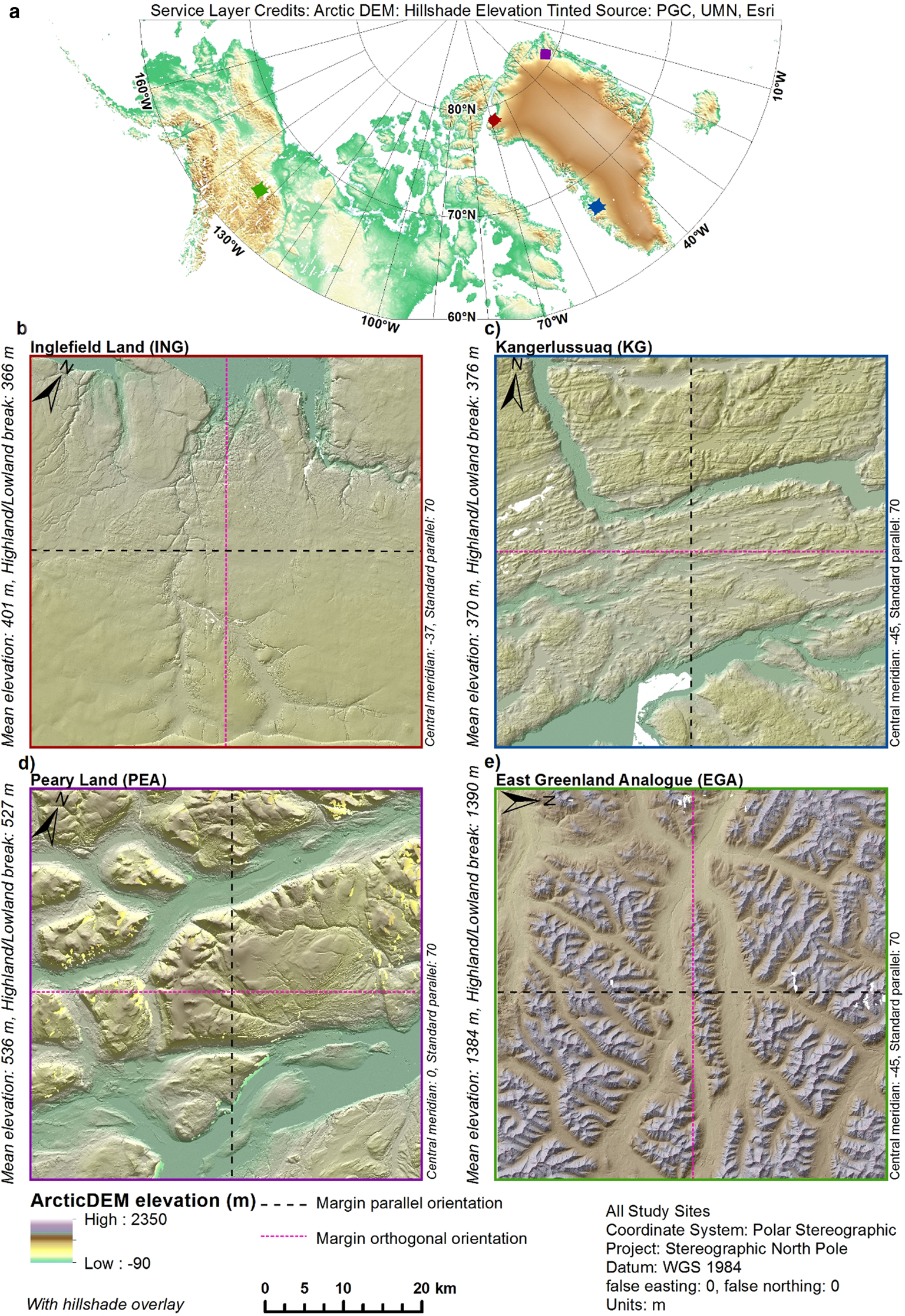
Fig. 1. Study site locations, topography and survey geometries. (a) Location of study sites. (b) Inglefield Land. (c) Kangerlussuaq. (d) Peary Land. (e) East Greenland Analogue (EGA).
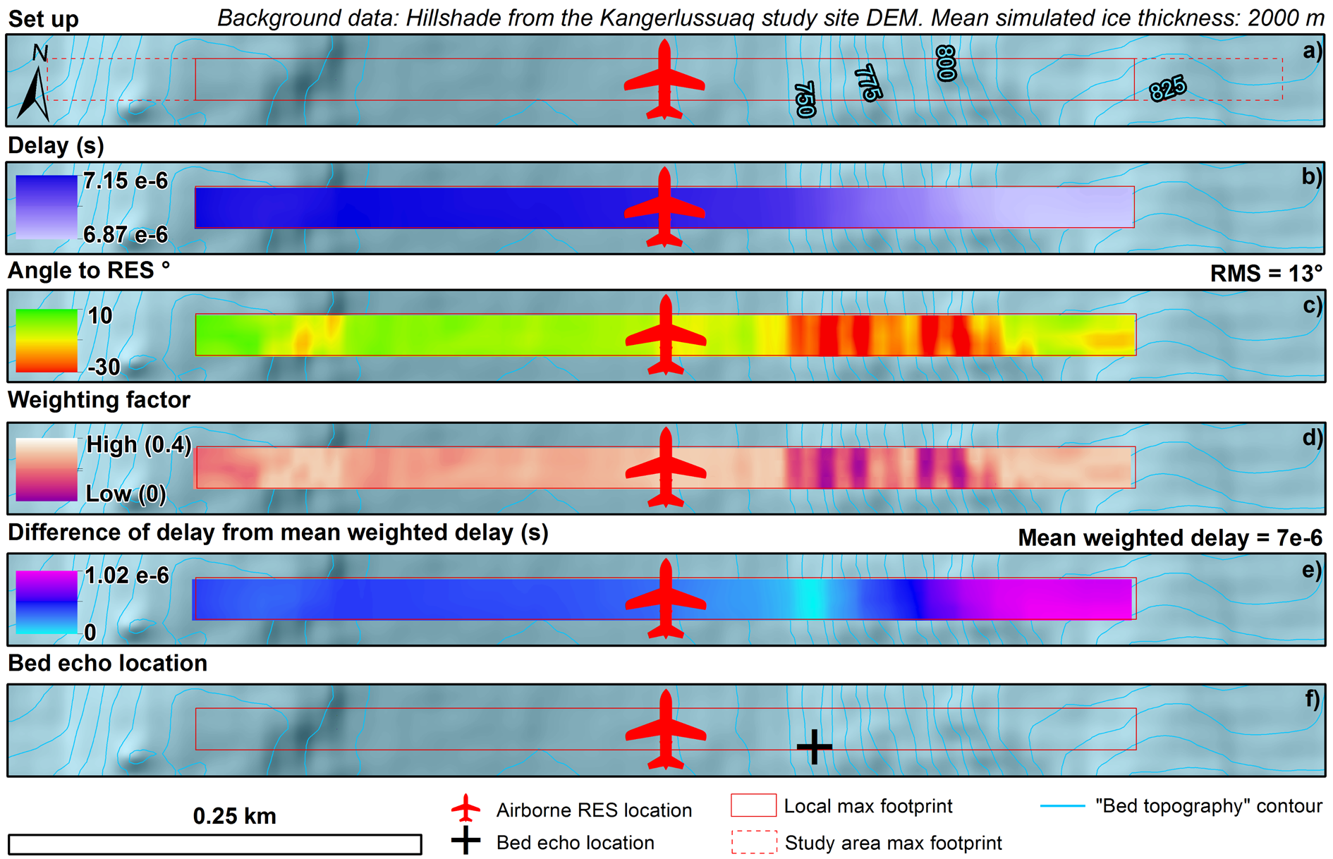
Fig. 2. Geospatial RES Survey simulator workflow. (a) Footprint calculation. (b) Delays. (c) Angle of surface to RES sensor. (d) Return weighting factor. (e) Difference of cell delay from the footprint mean weighted delay. (f) Most likely location of the brightest reflector.
Geospatial RES survey simulation
RES surveys and bed-elevation picking were simulated in ArcMap 10.5.1. Our simulation setup was based on NASA's Operation IceBridge flights using the MCoRDS system on a P-3 aircraft (CReSIS, 2018), because these comprise the majority of RES surveys conducted over the GrIS (Studinger and others, Reference Studinger, Koenig, Martin and Sonntag2010). The following model workflow is illustrated in Figure 2.
Flight-lines were simulated using typical IceBridge flight-line orientations, margin-parallel (MP) and margin-orthogonal (MO). MP flight-lines are typically used as ice-flux gates for estimating discharge as part of the mass-budget mass-balance approach (e.g. Rignot and Kanagaratnam, Reference Rignot and Kanagaratnam2006; Enderlin and others, Reference Enderlin2014; King and others, Reference King2018) and also comprise the principal inputs for mass-conservation-based interpolations (Morlighem and others, Reference Morlighem2017). MO flight-lines represent surveys designed to capture outlet-glacier thalwegs. Occasionally, IceBridge MP and MO lines have been combined to form grids (Studinger and others, Reference Studinger, Koenig, Martin and Sonntag2010). Extensive assessment of errors in both orientations is essential for quantifying uncertainty along and across gridded surveys.
To assess quality along each flight-line, points were plotted every 14 m, resembling the sample postings of an IceBridge survey. Raster layers were generated to simulate an ice-sheet surface. For each study site, an ice-sheet ‘interior’ surface was generated which was equivalent to the mean study site elevation plus 2000 m, to simulate mean ice thickness of ~2000 m. To simulate a ‘marginal’ situation, where the aircraft distance from the bed varies across the study site, a sloping ice-sheet-surface raster was generated which approximately replicated the surface slopes and surface elevations of the adjacent regions of the GrIS. For the EGA, approximate surface-elevation data were taken from the eastern margin of the GrIS near Helheim Glacier.
From the spatial location of a survey point and the 3D geometry of the DEM beneath it, we simulated the location of what would appear in a radargram as the brightest reflector, measured the elevation of this location and subsequently treated it as the ‘simulated nadir’ elevation.
In the along-track direction, footprint size was set to 25 m which replicated the along-track resolution of the MCoRDS system. For each along-track position, we searched across track within the maximum footprint width to investigate from where the echo originated, rather than taking the common assumption that it came from directly below the aircraft.
For every point, the maximum footprint width was calculated to represent the coarsest-resolution measurement that could be made at that point following the CReSIS Radar Depth Sounder report, 2018 (CReSIS, 2018). The maximum resolution, MaxFP, is related to the height of the aircraft above the ice-sheet surface Za and the maximum ice thickness for the study site h max, by
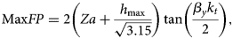
where βy is the beam width in radians (0.3) and kt is the approximate cross-track-windowing factor (1.3) (CReSIS, 2018). Once the maximum footprint for each survey point was generated, a localised maximum footprint for each point was calculated using Eqn (1), substituting h max with the maximum ice thickness within MaxFP at that point.
Within each local footprint, distances to and from the survey points were calculated trigonometrically and converted to delays by dividing by the speed of light (Fig. 2b). As the simulation was designed solely to determine the influence of topographic and survey geometry on the most probable location of a return, adjustments relating to physical properties of the radar pulse through ice were not parameterised.
For each footprint, we determined the RMS slope of the surface in the across-track direction. Subsequently, this RMS slope value was used as an estimate of the scattering-function width of the bed in each location, which we approximated as Gaussian (Schroeder and others, Reference Schroeder2016). At each cell, we used the angle of the surface with respect to the sensor and the estimated scattering-function width to weight the return from each cell (Fig. 2c).
From the assigned cell weightings, the mean weighted delay for the entire footprint was calculated accordingly (Fig. 2d). Mean weighted delays for each footprint were compared with the delay values for the cells within them, with the likely location of the brightest reflector being determined as the elevation cell whose delay either equalled or most closely matched the mean weighted delay (Figs 2e and f).
For actual surveys, returns are typically treated as though they come from directly beneath the aircraft. To simulate this, the elevation at the location of the brightest echo was extracted to the nadir position (Fig. 2f from the cross to the aircraft). Because the elevation at the likeliest location of the strongest return was expected to be different to the nadir elevation, it was termed the ‘simulated nadir elevation’. Once extracted, the simulated nadir elevation was differenced from the nadir elevation. This difference is referred to from herein as the ‘off-nadir elevation difference’.
Quantitative analysis of RES survey uncertainty
We calculated descriptive statistics for the off-nadir elevation differences for each study site to investigate the magnitude of RES uncertainty across the different types of landscape. We then further calculated descriptive statistics for the off-nadir elevation difference within elevation provinces so that any difference in measurements within highlands and lowlands could be investigated with no a priori assumptions of landscape features. Highland and lowland provinces were determined by reclassifying the study site DEMs into two classes based upon the natural breaks inherent in the data, so that elevation values were grouped into classes that maximise the differences between the means of the two classes (boundaries stated in Fig. 1).
For each MP flight-line, we measured valley cross-section, depth, width and area (referred to as CSA herein) from the DEM and the simulated elevation profiles. In order to semi-automate this process and keep the measurements consistent, we implemented the ‘findpeaks’ function in MATLAB which extracts ‘prominence’, the depth of a valley in cross-section, and ‘width at half-prominence’ (see Fig. 3 for examples). CSA was calculated as the trapezoidal approximation of the bottom half of each valley cross-section, using the edge locations of the width at half-prominence as the integration limits. We implemented this integration as each profile is made up of points separated by the sampling distance of the RES survey and the trapezoid width simulates this, as opposed to interpolating a curve to represent the valley cross-section. A final manual check was made to remove valley measurements from either the DEM profile or simulated elevation profile which did not have a corresponding measurement on the alternate profile.
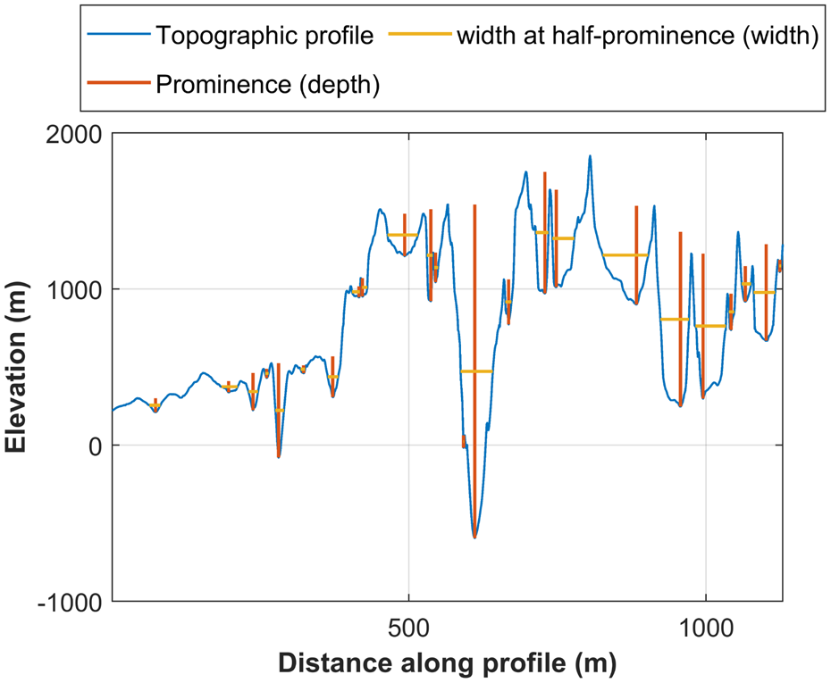
Fig. 3. Schematic representation of ‘findpeaks’ function to determine valley cross-section geometry.
Simulation measurement uncertainty
Both the DEM elevation value and the simulated nadir measurement at each point are subject to absolute and relative uncertainties in the ArcticDEM, which are currently estimated at <± 1 and 0.1 m, respectively (Porter and others, Reference Porter2018).
In reality, each simulated measurement would be subject to ‘ice bottom errors’ described by CReSIS (2018, pp. 26–27), and errors inherent in RES surveying highlighted by Lapazaran and others (Reference Lapazaran, Otero, Martín-Español and Navarro2016). These errors are typically on the order of tens of metres, and hence we acknowledge the additional scale of these errors throughout our interpretation of the ‘off-nadir elevation difference’ below.
Results
Synthetic RES survey results summary
In total, 2 647 090 bed measurements were simulated across the four study sites. The simulated bed measurements have a mean off-nadir elevation difference of −1.8 ± 11.6 m. Across all study sites, the mean and total off-nadir elevation difference are consistently negative. Importantly, this underestimation is spatially heterogeneous: greater mismeasurement occurs across highlands compared to lowlands, and extreme mismeasurements (>3σ from the mean) are likely to be over-estimates in lowlands as opposed to under-estimates in highlands. In addition, valley cross-section measurements show widespread under-estimation of valley depth and CSA, albeit high variation is observed in the measurement of these characteristics. In marginal simulations, where the maximum local footprint size is reduced, off-nadir elevation difference size is reduced and higher magnitude off-nadir elevation differences (>10 m) are less likely. Accordingly, mismeasurement of valley morphometry is also reduced.
Off-nadir elevation difference at the study-site scale
Negative bias in off-nadir elevation difference occurs across all study sites (Table 1). Both the sum of all off-nadir elevation differences across a study site and the mean off-nadir elevation difference are consistently negative. Sums of off-nadir elevation differences are more negative for MO simulations compared with their respective MP runs (Table 1). The EGA has the most negative total and mean off-nadir elevation difference in all simulations. Additionally, std dev. is greatest for the EGA; hence, elevation mismeasurement is greatest in such landscapes.
Table 1. Off-nadir elevation difference from DEM nadir elevation for all study sites and simulation set up
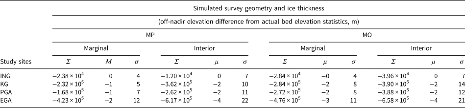
Σ is the sum, μ the mean and σ the standard off-nadir elevation difference.
Off-nadir elevation difference for individual survey points
Ordinary least-squares linear regression shows the simulated measured elevation to be on average 0.3% lower than the DEM elevation plus 0.3 m. RMSE from this regression also demonstrates that each simulated elevation is within 10.6 m of the DEM elevation, or ~0.1% of ice thickness.
There is no distinguishable relationship in the magnitude of the off-nadir elevation difference and ice thickness (Fig. 4). It can be seen in Figure 4 that survey point off-nadir elevation difference is predominantly negative, particularly where ice thickness is <500 m. As ice-thickness increases, off-nadir elevation differences are more often positive and their error as a percentage of ice thickness greatly reduces.
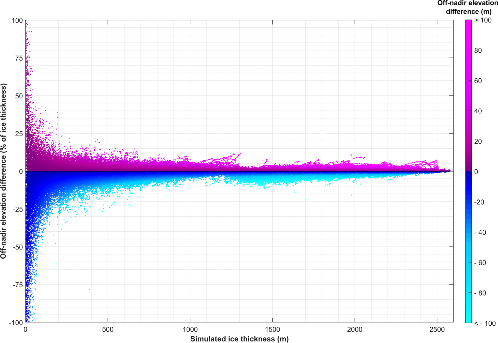
Fig. 4. Off-nadir elevation difference as a percentage of ice thickness against simulated ice thickness. Colour illustrates the off-nadir elevation difference values in metres.
Across all simulations, the probability of negative off-nadir elevation differences is greater for highlands than lowlands (Fig. 5 and skewness in Table S1). Metre-scale error (~0.1% of ice thickness) occurs for the majority of survey points (~80%, Fig. 5). Off-nadir elevation differences >10 m in scale (~1% of ice thickness) occur for ~20% of survey points. In lowlands, such off-nadir elevation differences are equally likely to be positive or negative, whereas in highlands, they are twice as likely to be negative than positive. Off-nadir elevation differences >100 m in scale (~10% of ice thickness) are rare (0.1% of measurements). However, as RES surveys sample many thousands of locations, they are not inconsequential. In our sampling for this paper, these extremely large off-nadir elevation differences were always negative in highlands but positive in lowlands.
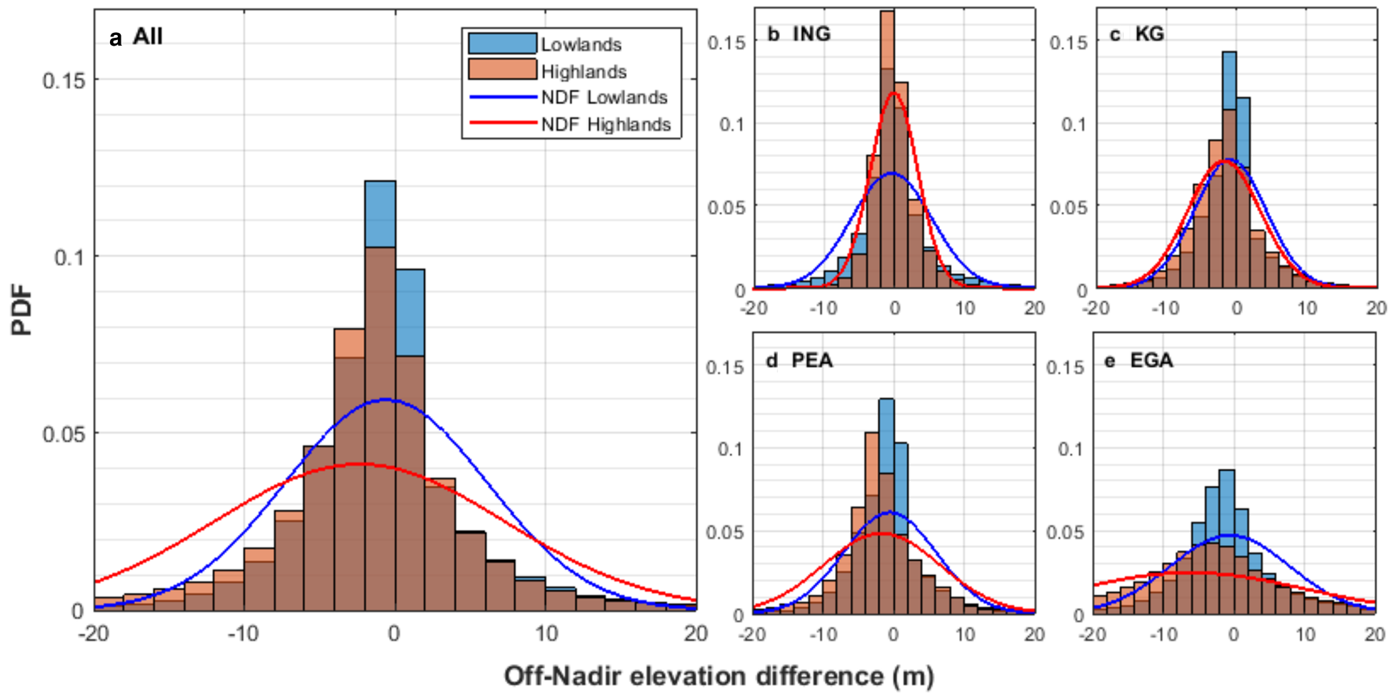
Fig. 5. Probability density functions for off-nadir elevation difference across all highland provinces and all lowland provinces. Bin size is 2 m. Normalized distribution functions are plotted as lines with colour corresponding to elevation province. (a) All points from MP marginal simulations. (b) Inglefield Land. (c) Kangerlussuaq. (d) Peary Land. (e) East Greenland Analogue.
Probability density functions also vary between study sites. Although MP marginal simulations generate a lower probability of high magnitude off-nadir elevation differences across all study sites and elevation provinces, the probability of negative 10 m-scale off-nadir elevation differences remains high for EGA highlands, with 30% of off-nadir elevation differences more than 10 m below zero.
Absolute values of off-nadir elevation difference mapped in Figure 6 highlight the spatial pattern of greater error in highlands as opposed to lowlands. Additionally, boundaries between highlands and lowlands, typically valley slopes, exhibited some of the largest errors, particularly for narrow valleys with varied orientation. Alpine topography typified by the EGA exhibits overall larger off-nadir elevation difference values in general compared to a landscape of areal scour such as Kangerlussuaq (overall darker colouration in Fig. 6).
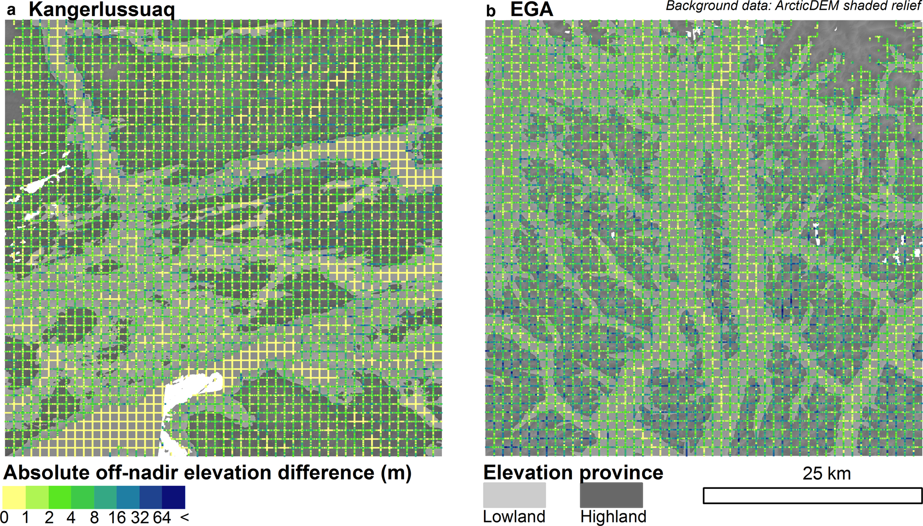
Fig. 6. Maps of absolute off-nadir elevation difference (coloured lines) across a landscape and provinces (grey shading) from marginal ice-thickness simulations. (a) Kangerlussuaq. (b) EGA.
Valley cross-section geometry errors
In total, 2145 valley cross-sections are identified across marginal MP flight-lines (summary statistics for all simulations in Table S2). Width, depth and CSA measurements are all found to be measured with a highly variable difference across all valley cross-sections (Table S2). However, simulated measurements of depth and CSA are predominantly negative, where ~70% of depth and ~55% of CSA measurements were under-estimates for interior simulations. Valley cross-section widths are under- and over-estimated in equal amounts. Finally, all the maximum magnitude differences in valley characteristics are negative.
Despite the large variation in measurement difference (~10 m), depth was largely under-estimated throughout, with the difference of valley-depth measurements increasing with total depth (Fig. 7). Although no clear trend is observed between valley area and depth difference, valley cross-sections with CSA >106 m2 exhibited greater under-estimates of depth than those between 105 and 106 m2.
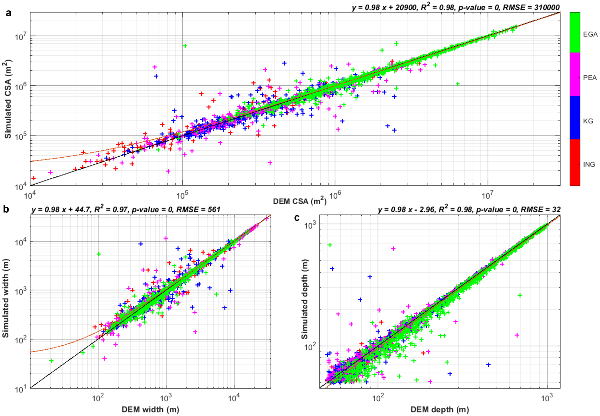
Fig. 7. Valley geometry measurement-accuracy assessment. All measurements from all MP flight-lines are plotted and study areas are colour coded. Linear regressions are plotted in dark red with equations at the top right of each plot; black line marks y = x. (a) Marginal ice-thickness simulation DEM valley CSA vs simulated valley CSA. (b) Marginal; DEM valley width vs simulated valley width. (c) Marginal; DEM valley depth vs simulated valley depth. Coefficients for interior setups in Table S3.
CSA mean differences were negative for all areas but Inglefield Land and the EGA interior simulation (Table S2). Figure 7 shows a large variation in simulated CSA and actual CSA. However, 54% of valley cross-sections fall below the equal match line (y = x). Off-nadir elevation differences from the actual CSA are lesser for larger valley cross-sections (CSA > 105 m2), yet are still predominantly negative (70%). The mean percentage difference in CSA for these large valley cross-sections is −3 ± 18%. For those smaller than 106 m2, mean CSA difference is always positive. Conversely, valley cross-sections larger than 106 m2 across all study sites and ice-thickness setups were smaller in RES-simulated bed-profiles compared with the DEM-derived profile.
Discussion
Spatial uncertainty in RES survey measurements
Measurement error due to off-nadir returns typically results in the under-estimation of bed elevation (Table 1). Preferential measurement of slopes orientated favourably with respect to the sensor location, as opposed to the immediate nadir location, results in most of the topography being under-estimated. Consequently, ice thicknesses derived from RES surveys are generally over-estimated. Although individual measurement error is modest at a given location (typically −1.8 ± 11.6 m), due to the many measurements made in a survey, these small off-nadir elevation differences accumulate to larger total over-estimation of ice thickness (Table 1). Additionally, for surveys over interior portions of an ice sheet, this may be further exacerbated due to the increased likelihood of larger errors in bed elevation measurement (Table 1). Furthermore, MO flight-lines should be treated with greater uncertainty than MP flight-lines as they exhibit larger mean off-nadir elevation difference and cumulative off-nadir elevation difference values (Table 1). As MO flight-lines typically constitute the predominant measurement of glacier centrelines, this has implications for the accuracy of such measurements and any subsequently derived metrics for ice dynamics and mass balance. Moreover, MO components of gridded surveys will likely be slightly less accurate than the MP components. However, all the above are dependent on the configuration of the subglacial topography being surveyed.
Widespread under-estimation of bed elevation is spatially heterogeneous. In highland areas, under-estimation is prevalent where local peaks and their slopes present as areas of highly variable orientation of the landscape with respect to the sensor (Fig. 8). This results in off-nadir returns from areas preferentially facing lower elevation, an effect that is exacerbated in areas where the mean orientation of the topography is parallel to the direction of flight, where topography predominantly slopes away from the sensor (Fig. 6). Conversely, in areas of low elevation, this bias is reduced and the likelihood of over-estimation of bed elevation is increased (Figs 5, 6 and 8, Table S1). In the bottoms of valleys, surface slopes are lower and less variable in orientation; therefore, regions of higher slope in valley bottoms have a greater influence on recorded nadir elevation, which is predominantly the valley sides (Fig. 8). Consequently, this is less of a problem in wider flatter valleys (Figs 6 and 8). Similarly to highlands, the orientation of lowland features fundamentally influences the magnitude of measurement off-nadir elevation difference. Flight-lines along a valley are more likely to be influenced by off-nadir returns from the valley sides, as opposed to flight-lines across valleys (Figs 6 and 8). However, the wider the valley, the lesser the impact orientation has on measurement error.
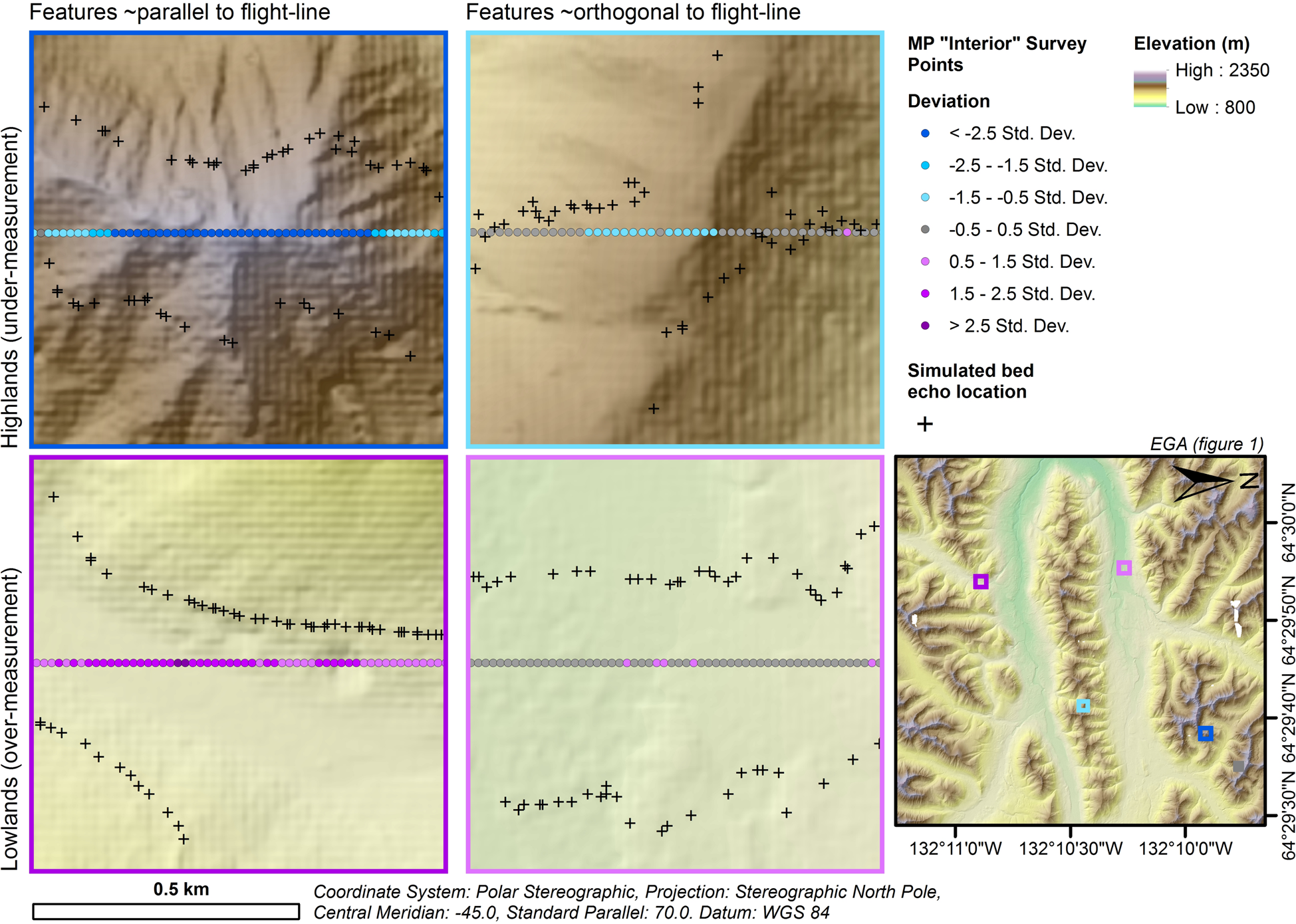
Fig. 8. Off-nadir elevation-difference magnitude and sign as a result of survey orientation; examples from EGA MP ‘interior’ simulation. (a) Highland elevations approximately parallel to flight-line orientation. (b) Highland elevations approximately orthogonal to flight-line orientation. (c) Lowland elevations approximately parallel to flight-line orientation. (d) Lowland elevations approximately orthogonal to flight-line orientation.
Spatial uncertainty in bed measurement alone can be seen to cause off-nadir elevation differences from the order of 1 to 100 m. While this error is modest compared to 10 m scale errors arising from physical conditions such as the ice–bed state (CReSIS, 2018), scattering and attenuation due to crevasses or subglacial or englacial meltwater (Paden and others, Reference Paden, Akins, Dunson, Allen and Gogineni2010), and errors arising from horizontal positioning (Lapazaran and others, Reference Lapazaran, Otero, Martín-Español and Navarro2016), it presents as a systematic bias which is also important to consider.
Potential for correction of RES survey measurement bias
As off-nadir elevation differences systematically under-estimate bed elevation, potential exists for ‘correction’ factors to be derived and applied to existing and future RES survey data conducted with the MCoRDS system simulated here. Here we explore the potential of developing corrections to counter off-nadir elevation difference errors.
Global elevation correction
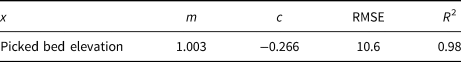
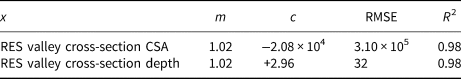
To broadly adjust picked bed elevations as a first-order correction of RES survey data, the ordinary least-squares regression mentioned previously may be used (coefficients in Table 2). This correction would alleviate the global negative bias and provide more accurate quantification of ice thickness and accordingly potential sea-level rise contribution from the ice sheet. Such a correction may be an appropriate step before widespread interpolation of bed topography.
Table 2. Coefficients for ordinary least-squares regression ‘global elevation correction’
Statistical topographic profile correction
Ice-thickness error in topographically-constrained outlet glaciers has far higher consequences for mass-balance estimation than the difference in ice thickness over largely static, highland areas (Enderlin and others, Reference Enderlin2014). Applying a statistical correction to flux-gate flight-lines, in effect to elevate under-estimated highland areas, may replicate the landscape better which, in turn, could generate more representative ice-flux and outlet-glacier-geometry estimates (Table 3; for other flight-line configurations and ice thicknesses, see Table S1).
Table 3. Potential correction factors for highlands and lowlands in marginal MP flight-lines based on subglacial landscape. For confidence intervals, x is the input elevation
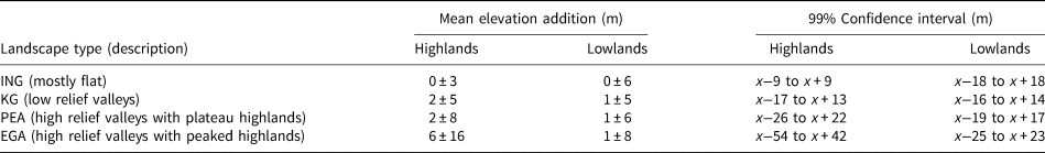
A statistical approach may be taken to simulate the boundaries of uncertainty in bed elevation and consequently valley depth and geometry, from which a range of discharge estimates may be calculated. Table 3 includes mean adjustments to be added to the input topography and confidence intervals for this method. Furthermore, this correction has the potential to minimise the propagation of mismeasurements of valley morphometry downstream by mass-conservation and ice-flux modelling. This would best be used for areas of subglacial topography like the EGA, which have the highest potential for producing higher magnitudes of error (Figs 6 and 8, Table S1). Up to 40% of points may deviate from the actual elevation by 10 m or more. Subglacial topography of this type is ubiquitous in the northwest and southeast of Greenland, which are the two most dominant sectors of the ice sheet in terms of ice discharge (Morlighem and others, Reference Morlighem2017; King and others, Reference King2018; Mouginot and others, Reference Mouginot2019). Therefore, large errors in bed measurement will have a compounding effect on the certainty of ice-discharge estimates made here. Improving the accuracy of bed topography is particularly important here, where outlet-glacier geometry has a significant influence on the stability and retreat potential of such glaciers (Catania and others, Reference Catania2018; Millan and others, Reference Millan2018).
Valley cross-section geometry correction
A more conservative approach to the statistical topographic profile correction suggested above could be to correct only the CSA and depth measurements which are used for ice-flux calculations (Fig. 7 and coefficients in Table 4). Although valleys with CSAs larger than 100 000 m2 are typically measured well, differences in the area are to the order of a few per cent which will influence total ice flux by the same ratio, assuming ice flux is equivalent to the CSA multiplied by the depth-averaged ice velocity through the CSA (Mouginot and others, Reference Mouginot2019). Nevertheless, ice velocity through a valley is calculated as a function of depth, which we find to be largely under-estimated even for larger valleys. Furthermore, valley CSA in this study is a conservative under-estimate of full-valley CSAs and so the full difference is expected to be greater. This bears significance for flight-lines used as ice-flux gates. Off-nadir elevation differences along these flight-lines, and the consequent misrepresentation of subglacial-valley geometry, have a direct effect on quantifying ice flux as part of the ice sheet's mass budget, modelling ice-sheet dynamics and deriving ice thickness via mass conservation (Enderlin and others, Reference Enderlin2014; Aschwanden and others, Reference Aschwanden, Fahnestock and Truffer2016; Morlighem and others, Reference Morlighem2017). Although mean off-nadir elevation difference is modest, the influence of large measurement errors across these flight-lines is substantial (PDFs in Fig. 4). Mass-budget studies using RES data to estimate ice discharge show bed-elevation errors to be ±30 m (Enderlin and others, Reference Enderlin2014; Mouginot and others, Reference Mouginot2019), which matches the RMSE for differences of valley depth found in our study for marginal measurements (Fig. 7). However, we estimate bed elevation errors for valleys further inland to be more than 50% greater (52.2 m on average, Table S3). Applying a correction to the depths and CSAs based on the regression functions calculated (Fig. 7) could be a ‘quick fix’ to improve ice-flux estimates by effectively expanding and deepening valleys accordingly.
Table 4. Coefficients for correcting CSA and depth for valley cross-sections in marginal RES survey profiles
Applying potential RES corrections to GrIS outlet glaciers
Taking the outlet glaciers of Helheim, Fenris and Midgard as a case study, we highlight the influence of potential RES-survey mismeasurement on outlet-glacier CSA and consequently the derived ice flux (Fig. 9). Here, we show the bed topography at an OIB flight-line location taken from BedMachine v3 (Morlighem and others, Reference Morlighem2017). When our valley cross-section correction is applied to the outlet glaciers, we find CSAs, and consequently ice fluxes, are typically under-estimated by 1 ± 1% (Fig. 9c). For mass-budget studies, this underestimation is an additional uncertainty to those previously determined for estimates of outlet-glacier ice flux (Enderlin and others, Reference Enderlin2014; King and others, Reference King2018). Furthermore, as CSA in this paper is an automated approximation for predominantly the bottom half of valleys, this is a conservative under-estimate. For the entire lateral extent of the valley, extending upwards from the valley sides to the ice surface, the percentage error will be higher as the elevation of highlands surrounding the valley is more often under-estimated at 10 m scales compared to similar scale overestimation of valley bottom elevation (Fig. 9b), effectively smoothing the bed profile and reducing overall bed elevation. Applying the statistical topographic profile correction derived from the probability density function for the EGA MP marginal experiment (Fig. 9, Table 3), it can be seen that the simulated topography could differ by ~50 m from the actual topography and the difference in valley CSA and consequently potential ice flux increases markedly, by as much as ±7% (Fig. 9).
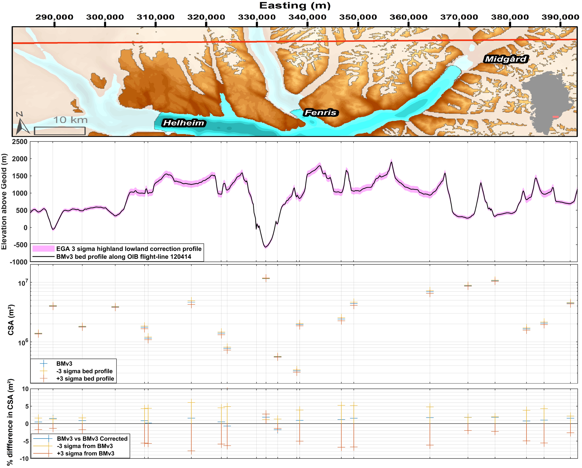
Fig. 9. (a) Red shows OIB spring 2012 flight 120414. Subglacial areas are indicated by the translucent white fill; background data are relief-shaded subglacial topography from BedMachine v3 (Morlighem and others, Reference Morlighem2017). Differences in bed topography (ab), CSA (c) and CSA percentage difference (d) along a flight-line using 99% confidence interval correction based on highland and lowland off-nadir elevation differences for the EGA study site. ‘BMv3 corrected’ uses the CSA correction derived from Figure 8b.
Implications for appreciation of outlet-glacier stability
Apparent smoothing of outlet-glacier valleys by off-nadir elevation difference typically results in smaller valley CSA being measured (Table S2, Fig. 7). This has implications for ice-flux estimations as these are derived in part using outlet-glacier CSA. Consequently, when valley profiles are corrected, so that the bottoms become deeper and the highlands higher, the CSA may increase, showing that current estimates of ice discharge may, in fact, be slightly too low.
Our study suggests that greatest mismeasurement of valley geometry occurs for interior, high-ice-thickness settings and for tributary glaciers to main outlets. These errors can scale up to hundreds of metres but are predominantly of the order of tens of metres. As these errors are propagated downstream in any mass-budgeting or mass-conservation analyses, errors become greatest at the glacier terminus and margin (Morlighem and others, Reference Morlighem2017; Millan and others, Reference Millan2018). Gravimetric measurements of outlet-glacier valley depth are reportedly deeper by tens to hundreds of metres than corresponding depths in BedMachine v3 (Millan and others, Reference Millan2018). This could in part be explained by the results in our study where valley depth is being under-estimated and subsequently carried downstream in interpolation. Accurate determination of outlet-glacier valley depth is of particular importance when assessing outlet-glacier stability, as this is often highly dependent on bed geometry (Choi and others, Reference Choi, Morlighem, Rignot, Mouginot and Wood2017; Catania and others, Reference Catania2018).
Mismeasurement of outlet-glacier valley geometry may complicate predictions of outlet-glacier stability. The depth and gradient of the beds of GrIS outlet glaciers determine whether the glacier may be exposed to warm Atlantic Water and if they are able to establish a new, stable grounding-line position after the initiation of retreat (Catania and others, Reference Catania2018). Glaciers such as Umiamako Isbrae and Kangilerngata Sermia have grounding-line depths, 264 and 260 m below sea level respectively, within the potential depth error ranges presented in Table S2 that could make them susceptible to ingress of Atlantic Water into their fjords (Choi and others, Reference Choi, Morlighem, Rignot, Mouginot and Wood2017; Catania and others, Reference Catania2018). Additionally, the portion of the bed that is retrograde for some glaciers may not be adequately captured by under-estimated valley depths and bed topography derived from erroneous inputs. This important condition is reported for Skinfaxe Glacier and Qajuuttap Sermia when using gravimetric measurements, yet, in BedMachine v3 which is derived from RES data, both glaciers have relatively flat beds and are grounded close to sea level (Millan and others, Reference Millan2018). Consistent under-estimation of depth also poses additional uncertainty when considering how much of the ice-sheet bed is grounded below sea level. Ikertivaq and North Kogebugt Glaciers have beds below sea level in gravimetric data but not in RES-derived bed topography, with depth measurements differing by a magnitude of 100 m (Millan and others, Reference Millan2018). While underestimation of depth was typically found to be an order of magnitude less than this, potentially more common mismeasurements to the order of 10 m are enough to differentiate whether these glaciers are grounded below sea level or not. Finally, the extra tens of metres that may be gained in depth in cases within one std dev. of the mean depth difference may alter predictions as to whether a glacier is at the floatation point, further influencing predictions of glacier stability (McMillan and others, Reference McMillan2014). All of the glaciers mentioned above are found in the southeast and northwest sectors of the GrIS, which as previously mentioned exhibit similar topography to the EGA site used in our study. Consequently, these areas are subject to heightened probability of larger mismeasurements of bed topography.
Conclusions
• We have demonstrated a systematic underestimation bias of subglacial elevation inherent to RES surveying, termed off-nadir elevation difference (mean = 1.8 ± 11.6 m), which implies current estimates of ice thickness are slightly high.
• We find CSA and consequently ice flux for outlet glaciers across the GrIS in landscapes similar to the EGA site presented here have typically been under-estimated by ~−3 ± 18%, potentially increasing up to 5% up-glacier.
• Widespread overestimation of valley bottom elevation may have implications for our appreciation of outlet-glacier stability.
• We highlight three potential corrections for RES survey data, namely: global elevation correction, statistical topographic profile correction and valley cross-section geometry correction.
Supplementary material
The supplementary material for this article can be found at https://doi.org/10.1017/aog.2020.35.
Acknowledgements
OTB was funded by the NERC GW4+ DTP studentship NE/L002434/1. Geospatial support for this work was provided by the Polar Geospatial Center under NSF-OPP awards 1043681 and 1559691. DEMs were provided by the Polar Geospatial Center under NSF-OPP awards 1043681, 1559691, and 1542736. We acknowledge the use of data and/or data products from CReSIS generated with support from the University of Kansas, NSF grant ANT-0424589 and NASA Operation IceBridge grant NNX16AH54G. We thank Robert Bingham for serving as the editor of this manuscript. We also thank Martin Siegert and one anonymous reviewer for their comments and feedback which greatly improved this manuscript.


 Open access