


1. Introduction
1.1 Monotonic increase of differential entropy
Let
 $X, Y$
be two independent random variables with densities in
$X, Y$
be two independent random variables with densities in
 $\mathbb{R}$
. The differential entropy of
$\mathbb{R}$
. The differential entropy of
 $X$
, having density
$X$
, having density
 $f$
, is
$f$
, is
 \begin{equation*} h(X) = -\int _{\mathbb {R}}{f(x)\log {f(x)}dx} \end{equation*}
and similarly for
 $Y$
. Throughout
$Y$
. Throughout
 $`\log$
’ denotes the natural logarithm.
$`\log$
’ denotes the natural logarithm.
The entropy power inequality (EPI) plays a central role in information theory. It goes back to Shannon [Reference Shannon15] and was first proven in full generality by Stam [Reference Stam16]. It asserts that
 \begin{equation} N(X+Y) \geq N(X) + N(Y), \end{equation}
where
 $N(X)$
is the entropy power of
$N(X)$
is the entropy power of
 $X$
:
$X$
:
 \begin{equation*} N(X) = \frac {1}{2 \pi e}e^{2h(X)}. \end{equation*}
If
 $X_1,X_2$
are identically distributed, (1) can be rewritten as
$X_1,X_2$
are identically distributed, (1) can be rewritten as
 \begin{equation} h(X_1+X_2) \geq h(X_1) + \frac{1}{2}\log{2}. \end{equation}
The EPI is also connected with and has applications in probability theory. The following generalisation is due to Artstein, Ball, Barthe and Naor [Reference Artstein, Ball, Barthe and Naor1]: If
 $\{X_i\}_{i=1}^{n+1}$
are continuous, i.i.d. random variables then
$\{X_i\}_{i=1}^{n+1}$
are continuous, i.i.d. random variables then
 \begin{equation} h\left(\frac{1}{\sqrt{n+1}}\sum _{i=1}^{n+1}{X_i}\right) \geq h\left(\frac{1}{\sqrt{n}}\sum _{i=1}^{n}{X_i}\right). \end{equation}
This is the monotonic increase of entropy along the central limit theorem [Reference Barron2]. The main result of this paper may be seen as an approximate, discrete analogue of (3).
1.2 Sumset theory for entropy
There has been interest in formulating discrete analogues of the EPI from various perspectives [Reference Haghighatshoar, Abbe and Telatar7–Reference Harremoés and Vignat9, Reference Woo and Madiman20]. It is not hard to see that the exact statement (2) can not hold for all discrete random variables by considering deterministic (or even close to deterministic) random variables.
Suppose
 $G$
is an additive abelian group and
$G$
is an additive abelian group and
 $X$
is a random variable supported on a discrete (finite or countable) subset
$X$
is a random variable supported on a discrete (finite or countable) subset
 $A$
of
$A$
of
 $G$
with probability mass function (p.m.f.)
$G$
with probability mass function (p.m.f.)
 $p$
on
$p$
on
 $G$
. The Shannon entropy, or simply entropy of
$G$
. The Shannon entropy, or simply entropy of
 $X$
is
$X$
is
 \begin{equation} H(X) = -\sum _{x \in A}{p(x)\log{p(x)}}. \end{equation}
Tao [Reference Tao17] proved that if
 $G$
is torsion-free and
$G$
is torsion-free and
 $X$
takes finitely many values then
$X$
takes finitely many values then
 \begin{equation} H(X_1+X_2) \geq H(X_1) + \frac{1}{2}\log{2} - o(1), \end{equation}
where
 $X_1, X_2$
are independent copies of
$X_1, X_2$
are independent copies of
 $X$
and the
$X$
and the
 $o(1)$
-term vanishes as the entropy of
$o(1)$
-term vanishes as the entropy of
 $X$
tends to infinity. That work explores the connection between additive combinatorics and entropy, which was identified by Tao and Vu in the unpublished notes [Reference Tao and Vu18] and by Ruzsa [Reference Ruzsa14]. The main idea is that random variables in
$X$
tends to infinity. That work explores the connection between additive combinatorics and entropy, which was identified by Tao and Vu in the unpublished notes [Reference Tao and Vu18] and by Ruzsa [Reference Ruzsa14]. The main idea is that random variables in
 $G$
may be associated with subsets
$G$
may be associated with subsets
 $A$
of
$A$
of
 $G$
: By the asymptotic equipartition property [Reference Cover and Thomas4], there is a set
$G$
: By the asymptotic equipartition property [Reference Cover and Thomas4], there is a set
 $A_n$
(the typical set) such that if
$A_n$
(the typical set) such that if
 $X_1,\ldots,X_n$
are i.i.d. copies of
$X_1,\ldots,X_n$
are i.i.d. copies of
 $X$
, then
$X$
, then
 $(X_1,\ldots,X_n)$
is approximately uniformly distributed on
$(X_1,\ldots,X_n)$
is approximately uniformly distributed on
 $A_n$
and
$A_n$
and
 $|A_n| = e^{n(H(X) + o(1))}.$
Hence, given an inequality involving cardinalities of sumsets, it is natural to guess that a counterpart statement holds true for random variables if the logarithm of the cardinality is replaced by the entropy.
$|A_n| = e^{n(H(X) + o(1))}.$
Hence, given an inequality involving cardinalities of sumsets, it is natural to guess that a counterpart statement holds true for random variables if the logarithm of the cardinality is replaced by the entropy.
Exploring this connection, Tao [Reference Tao17] proved an inverse theorem for entropy, which characterises random variables for which the addition of an independent copy does not increase the entropy by much. This is the entropic analogue of the inverse Freiman theorem [Reference Tao and Vu19] from additive combinatorics, which characterises sets for which the sumset is not much bigger than the set itself. The discrete EPI (5) is a consequence of the inverse theorem for entropy.
Furthermore, it was conjectured in [Reference Tao17] that for any
 $n \geq 2$
and
$n \geq 2$
and
 $\epsilon \gt 0$
 \begin{equation} H(X_1+\cdots +X_{n+1}) \geq H(X_1+\cdots +X_{n}) + \frac{1}{2}\log{\Bigl (\frac{n+1}{n}\Bigr )} - \epsilon, \end{equation}
provided that
 $H(X)$
is large enough depending on
$H(X)$
is large enough depending on
 $n$
and
$n$
and
 $\epsilon$
, where
$\epsilon$
, where
 $\{X_i\}_{i=1}^{n+1}$
are i.i.d. copies of
$\{X_i\}_{i=1}^{n+1}$
are i.i.d. copies of
 $X$
.
$X$
.
We will prove that the conjecture (6) holds true for log-concave random variables on the integers. An important step in the proof of (5) is reduction to the continuous setting by approximation of the continuous density with a discrete p.m.f.; we briefly outline these key points from that proof in Section 1.3 below as we are going to take a similar approach.
A discrete entropic central limit theorem was recently established in [Reference Gavalakis and Kontoyiannis6]. A discussion relating the above conjecture to the convergence of Shannon entropy to its maximum in analogy with (3) may be found there.
It has also been of interest to establish finite bounds for the
 $o(1)$
-term [Reference Haghighatshoar, Abbe and Telatar7, Reference Woo and Madiman20]. Our proofs yield explicit rates for the
$o(1)$
-term [Reference Haghighatshoar, Abbe and Telatar7, Reference Woo and Madiman20]. Our proofs yield explicit rates for the
 $o(1)$
-terms, which are exponential in
$o(1)$
-terms, which are exponential in
 $H(X_1)$
.
$H(X_1)$
.
The class of discrete log-concave distributions has been considered recently by Bobkov, Marsiglietti and Melbourne [Reference Bobkov, Marsiglietti and Melbourne3] in connection with the EPI. In particular, discrete analogues of (1) were proved for this class. In addition, sharp upper and lower bounds on the maximum probability of discrete log-concave random variables in terms of their variance were provided, which we are going to use in the proofs (see Lemma 5 below). Although log-concavity is a strong assumption in that it implies, for example, connected support set and moments of all orders, many important distributions are log-concave, e.g. Bernoulli, Poisson, geometric, negative binomial and others.
1.3 Main results and proof ideas
The first step in the proof method of [Reference Tao17, Theorem 1.9] is to assume that
 $H(X_1+X_2) \leq H(X_1) + \frac{1}{2}\log{2} - \epsilon .$
Then, because of [Reference Tao17, Theorem 1.8], proving the result for random variables
$H(X_1+X_2) \leq H(X_1) + \frac{1}{2}\log{2} - \epsilon .$
Then, because of [Reference Tao17, Theorem 1.8], proving the result for random variables
 $X$
that can be expressed as a sum
$X$
that can be expressed as a sum
 $Z+U$
, where
$Z+U$
, where
 $Z$
is a random variable with entropy
$Z$
is a random variable with entropy
 $O(1)$
and
$O(1)$
and
 $U$
is a uniform on a large arithmetic progression, say
$U$
is a uniform on a large arithmetic progression, say
 $P$
, suffices to get a contradiction. Such random variables satisfy, for every
$P$
, suffices to get a contradiction. Such random variables satisfy, for every
 $x$
,
$x$
,
 \begin{equation} \mathbb{P}(X = x) \leq \frac{C}{|P|} \end{equation}
for some absolute constant
 $C$
. Using tools from the theory of sum sets, it is shown that it suffices to consider random variables that take values in a finite subset of the integers. For such random variables that satisfy (7), the smoothness property
$C$
. Using tools from the theory of sum sets, it is shown that it suffices to consider random variables that take values in a finite subset of the integers. For such random variables that satisfy (7), the smoothness property
 \begin{equation} \|p_{X_1+X_2} - p_{X_1+X_2+1}\|_{\textrm{TV}} \to 0 \end{equation}
as
 $H(X) \to \infty$
is established, where
$H(X) \to \infty$
is established, where
 $p_{X_1+X_2}, p_{X_1+X_2+1}$
are the p.m.f.s of
$p_{X_1+X_2}, p_{X_1+X_2+1}$
are the p.m.f.s of
 $X_1+X_2$
and
$X_1+X_2$
and
 $X_1+X_2+1$
, respectively, and
$X_1+X_2+1$
, respectively, and
 $\|\cdot \|_{\textrm{TV}}$
is the total variation distance defined in (15) below. Using this, it is shown that
$\|\cdot \|_{\textrm{TV}}$
is the total variation distance defined in (15) below. Using this, it is shown that
 \begin{equation} h(X_1+X_2+U_1+U_2) = H(X_1+X_2) + o(1), \end{equation}
as
 $H(X) \to \infty,$
where
$H(X) \to \infty,$
where
 $U_1,U_2$
are independent continuous uniforms on
$U_1,U_2$
are independent continuous uniforms on
 $(0,1).$
The EPI for continuous random variables is then invoked.
$(0,1).$
The EPI for continuous random variables is then invoked.
The tools that we use are rather probabilistic– our proofs lack any additive combinatorial arguments as we already work with random variables on the integers, which have connected support set. An important technical step in our case is to show that any log-concave random variable
 $X$
on the integers satisfies
$X$
on the integers satisfies
 \begin{equation*} \|p_X- p_{X+1}\|_{\textrm {TV}} \to 0 \end{equation*}
as
 $H(X) \to \infty$
. Using this we show a generalisation of (9), our main technical tool:
$H(X) \to \infty$
. Using this we show a generalisation of (9), our main technical tool:
Theorem 1.
Let
 $n \geq 1$
and suppose
$n \geq 1$
and suppose
 $X_1,\ldots,X_n$
are i.i.d. log-concave random variables on the integers with common variance
$X_1,\ldots,X_n$
are i.i.d. log-concave random variables on the integers with common variance
 $\sigma ^2.$
Let
$\sigma ^2.$
Let
 $U_1,\ldots,U_n$
be continuous i.i.d. uniforms on
$U_1,\ldots,U_n$
be continuous i.i.d. uniforms on
 $(0,1).$
Then
$(0,1).$
Then
 \begin{equation} h(X_1+\cdots +X_n+U_1+\cdots +U_n) = H(X_1+\cdots +X_n) + o(1), \end{equation}
where the
 $o(1)$
-term vanishes as
$o(1)$
-term vanishes as
 $\sigma ^2 \to \infty$
depending on
$\sigma ^2 \to \infty$
depending on
 $n$
. In fact, this term can be bounded absolutely by
$n$
. In fact, this term can be bounded absolutely by
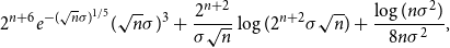 \begin{equation} 2^{n+6} e^{-(\sqrt{n}\sigma )^{1/5}} (\sqrt{n}\sigma )^{3} + \frac{2^{n+2}}{\sigma \sqrt{n}}\log (2^{n+2}\sigma \sqrt{n}) +\frac{\log{(n\sigma ^2)}}{8n\sigma ^2}, \end{equation}
provided that
 $\sigma \gt \max \{2^{n+2}/\sqrt{n},3^7/\sqrt{n}\}$
.
$\sigma \gt \max \{2^{n+2}/\sqrt{n},3^7/\sqrt{n}\}$
.
Remark 2. Note that always,
 $H(X) \to \infty$
implies
$H(X) \to \infty$
implies
 $\sigma ^2 \to \infty,$
since by the maximum entropy property of the Gaussian distribution [Reference Cover and Thomas4]
$\sigma ^2 \to \infty,$
since by the maximum entropy property of the Gaussian distribution [Reference Cover and Thomas4]
 \begin{equation} H(X) = h(X+U) \leq \frac{1}{2}\log{\left(2\pi e\sigma ^2(1+\frac{1}{12})\right)}, \end{equation}
where
 $U$
is an independent continuous uniform on
$U$
is an independent continuous uniform on
 $(0,1)$
. Conversely, for the class of log-concave random variables
$(0,1)$
. Conversely, for the class of log-concave random variables
 $\sigma \to \infty$
implies
$\sigma \to \infty$
implies
 $H(X) \to \infty$
, e.g. by Proposition 7 and Lemma 5. Indeed these give a quantitative comparison between
$H(X) \to \infty$
, e.g. by Proposition 7 and Lemma 5. Indeed these give a quantitative comparison between
 $H(X)$
and
$H(X)$
and
 $\sigma ^2=\textrm{Var}(X)$
for log-concave random variables:
$\sigma ^2=\textrm{Var}(X)$
for log-concave random variables:
 $H(X) \geq \log{\sigma }$
for
$H(X) \geq \log{\sigma }$
for
 $\sigma \geq 1$
.
$\sigma \geq 1$
.
Our main tools are first, to approximate the density of the log-concave sum convolved with the sum of
 $n$
continuous uniforms with the discrete p.m.f. (Lemma 8) and second, to show a type of concentration for the “information density”,
$n$
continuous uniforms with the discrete p.m.f. (Lemma 8) and second, to show a type of concentration for the “information density”,
 $-\log{p(S_n)},$
using Lemma 9. It is a standard argument to show that log-concave p.m.f.s have exponential tails, since the sum of the probabilities is convergent. Lemma 9 is a slight improvement in that it provides a bound for the ratio depending on the variance.
$-\log{p(S_n)},$
using Lemma 9. It is a standard argument to show that log-concave p.m.f.s have exponential tails, since the sum of the probabilities is convergent. Lemma 9 is a slight improvement in that it provides a bound for the ratio depending on the variance.
By an application of the generalised EPI for continuous random variables, we show that the conjecture (6) is true for log-concave random variables on the integers, with an explicit dependence between
 $H(X)$
and
$H(X)$
and
 $\epsilon .$
Our main result is:
$\epsilon .$
Our main result is:
Theorem 3.
Let
 $n \geq 1$
and
$n \geq 1$
and
 $\epsilon \in (0,1)$
. Suppose
$\epsilon \in (0,1)$
. Suppose
 $X_1,\ldots,X_n$
are i.i.d. log-concave random variables on the integers. Then if
$X_1,\ldots,X_n$
are i.i.d. log-concave random variables on the integers. Then if
 $H(X_1)$
is sufficiently large depending on
$H(X_1)$
is sufficiently large depending on
 $n$
and
$n$
and
 $\epsilon$
,
$\epsilon$
,
 \begin{equation} H(X_1+\cdots +X_{n+1}) \geq H(X_1+\cdots +X_{n}) + \frac{1}{2}\log{\Bigl (\frac{n+1}{n}\Bigr )} - \epsilon . \end{equation}
In fact, for (
13
) to hold it suffices to take
 $H(X_1) \geq \log{\frac{2}{\epsilon }} + \log{\log{\frac{2}{\epsilon }}} + n + 27.$
The proofs of Theorems 1 and 3 are given in Section 3. Before that, in Section 2 below, we prove some preliminary facts about discrete, log-concave random variables.
For
 $n=1,$
the lower bound for
$n=1,$
the lower bound for
 $H(X_1)$
given by Theorem 3 for the case of log-concave random variables on the integers is a significant improvement on the lower bound that can be obtained from the proof given in [Reference Tao17] for discrete random variables in a torsion-free group, which is
$H(X_1)$
given by Theorem 3 for the case of log-concave random variables on the integers is a significant improvement on the lower bound that can be obtained from the proof given in [Reference Tao17] for discrete random variables in a torsion-free group, which is
 $\Omega \Bigl ({\frac{1}{\epsilon }}^{{\frac{1}{\epsilon }}^{\frac{1}{\epsilon }}}\Bigr )$
.
$\Omega \Bigl ({\frac{1}{\epsilon }}^{{\frac{1}{\epsilon }}^{\frac{1}{\epsilon }}}\Bigr )$
.
Finally, let us note that Theorem 1 is a strong result: Although we suspect that the assumption of log-concavity may be relaxed, we do not expect it to hold in much greater generality; we believe that some structural conditions on the random variables should be necessary.
2. Notation and preliminaries
For a random variable
 $X$
with p.m.f.
$X$
with p.m.f.
 $p$
on the integers denote
$p$
on the integers denote
 \begin{equation} q \;:\!=\; \sum _{k \in \mathbb{Z}}\min \{p(k),p(k+1)\}. \end{equation}
The parameter
 $q$
defined above plays an important role in a technique known as Bernoulli part decomposition, which has been used in [Reference Davis and McDonald5, Reference McDonald12, Reference Mineka13] to prove local limit theorems. It was also used in [Reference Gavalakis and Kontoyiannis6] to prove the discrete entropic CLT mentioned in the Introduction.
$q$
defined above plays an important role in a technique known as Bernoulli part decomposition, which has been used in [Reference Davis and McDonald5, Reference McDonald12, Reference Mineka13] to prove local limit theorems. It was also used in [Reference Gavalakis and Kontoyiannis6] to prove the discrete entropic CLT mentioned in the Introduction.
In the present article, we use
 $1-q$
as a measure of smoothness of a p.m.f. on the integers. In what follows we will also write
$1-q$
as a measure of smoothness of a p.m.f. on the integers. In what follows we will also write
 $q(p)$
to emphasise the dependence on the p.m.f.
$q(p)$
to emphasise the dependence on the p.m.f.
 $p$
.
$p$
.
For two p.m.f.s on the integers
 $p_1$
and
$p_1$
and
 $p_2$
, we use the notation
$p_2$
, we use the notation
 \begin{equation*}\|p_1 - p_2\|_{1} \;:\!=\; \sum _{k \in \mathbb {Z}}{|p_1(k)-p_2(k)|}\end{equation*}
for the
 $\ell _1$
-distance between
$\ell _1$
-distance between
 $p_1$
and
$p_1$
and
 $p_2$
and
$p_2$
and
 \begin{equation} \|p_1 - p_2\|_{\textrm{TV}} \;:\!=\; \frac{1}{2}\|p_1 - p_2\|_{1} \end{equation}
for the total variation distance.
Proposition 4.
Suppose
 $X$
has p.m.f.
$X$
has p.m.f.
 $p_X$
on
$p_X$
on
 $\mathbb{Z}$
and let
$\mathbb{Z}$
and let
 $q = \sum _{k \in \mathbb{Z}}{\min{\{p_X(k),p_X(k+1)\}}}$
. Then
$q = \sum _{k \in \mathbb{Z}}{\min{\{p_X(k),p_X(k+1)\}}}$
. Then
 \begin{equation*}\|p_X - p_{X+1}\|_{\textrm {TV}} = 1-q.\end{equation*}
Proof. Since
 $|a-b| = a + b - 2\min{\{a,b\}}$
,
$|a-b| = a + b - 2\min{\{a,b\}}$
,
 \begin{equation*} \|p_X-p_{X+1}\|_1 = \sum _{k\in \mathbb {Z}}{|p_X(k) - p_X(k+1)|} = 2 - 2\sum _{k \in \mathbb {Z}}{\min {\{p_X(k),p_X(k+1)\}}} = 2(1-q). \end{equation*}
The result follows.
A p.m.f.
 $p$
on
$p$
on
 $\mathbb{Z}$
is called log-concave, if for any
$\mathbb{Z}$
is called log-concave, if for any
 $k \in \mathbb{Z}$
 \begin{equation} p(k)^2 \geq p(k-1)p(k+1). \end{equation}
If a random variable
 $X$
is distributed according to a log-concave p.m.f. we say that
$X$
is distributed according to a log-concave p.m.f. we say that
 $X$
is log-concave. Throughout we suppose that
$X$
is log-concave. Throughout we suppose that
 $X_1,\ldots,X_n$
are i.i.d. random variables having a log-concave p.m.f. on the integers,
$X_1,\ldots,X_n$
are i.i.d. random variables having a log-concave p.m.f. on the integers,
 $p$
, common variance
$p$
, common variance
 $\sigma ^2$
and denote their sum with
$\sigma ^2$
and denote their sum with
 $S_n$
. Also, we denote
$S_n$
. Also, we denote
 \begin{equation*} p_{{\textrm {max}}} = p_{{\textrm {max}}}(X) \;:\!=\; \sup _k{\mathbb {P}(X = k)} \end{equation*}
and write
 \begin{equation} N_{\textrm{max}} = N_{\textrm{max}}(X) \;:\!=\; \max \{k \in \mathbb{Z}\;:\; p(k) = p_{{\textrm{max}}}\}, \end{equation}
i.e.
 $N_{\textrm{max}}$
is the last
$N_{\textrm{max}}$
is the last
 $k \in \mathbb{Z}$
for which the maximum probability is achieved. We will make use of the following bound from [Reference Bobkov, Marsiglietti and Melbourne3]:
$k \in \mathbb{Z}$
for which the maximum probability is achieved. We will make use of the following bound from [Reference Bobkov, Marsiglietti and Melbourne3]:
Lemma 5.
Suppose
 $X$
has discrete log-concave distribution with
$X$
has discrete log-concave distribution with
 $\sigma ^2 = \textrm{Var}{(X)} \geq 1.$
Then
$\sigma ^2 = \textrm{Var}{(X)} \geq 1.$
Then
 \begin{equation} \frac{1}{4\sigma } \leq p_{{\textrm{max}}} \leq \frac{1}{\sigma }. \end{equation}
Proof. Follows immediately from [Reference Bobkov, Marsiglietti and Melbourne3, Theorem 1.1.].
Proposition 6.
Let
 $X$
be a log-concave random variable on the integers with mean
$X$
be a log-concave random variable on the integers with mean
 $\mu \in \mathbb{R}$
and variance
$\mu \in \mathbb{R}$
and variance
 $\sigma ^2$
, and let
$\sigma ^2$
, and let
 $\delta \gt 0$
. Then, if
$\delta \gt 0$
. Then, if
 $\sigma \gt 4^{1/2\delta },$
 \begin{equation} |N_{\textrm{max}} - \mu | \lt \sigma ^{3/2+\delta } +1. \end{equation}
Proof. Suppose for contradiction that
 $ |N_{\textrm{max}} - \mu | \geq \sigma ^{3/2+\delta }+1$
. Then, using (18),
$ |N_{\textrm{max}} - \mu | \geq \sigma ^{3/2+\delta }+1$
. Then, using (18),
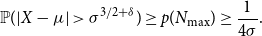 \begin{equation*} \mathbb {P}(|X - \mu | \gt \sigma ^{3/2+\delta }) \geq p(N_{\textrm {max}}) \geq \frac {1}{4\sigma }. \end{equation*}
But Chebyshev’s inequality implies
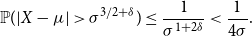 \begin{equation*} \mathbb {P}(|X - \mu | \gt \sigma ^{3/2+\delta }) \leq \frac {1}{\sigma ^{1 + 2\delta }} \lt \frac {1}{4\sigma }. \end{equation*}
Below we show that for any integer-valued random variable
 $X$
,
$X$
,
 $q \to 1$
implies
$q \to 1$
implies
 $H(X) \to \infty$
. It is not hard to see that the converse is not always true, i.e.
$H(X) \to \infty$
. It is not hard to see that the converse is not always true, i.e.
 $H(X) \to \infty$
does not necessarily imply
$H(X) \to \infty$
does not necessarily imply
 $q \to 1$
: Consider a random variable with a mass of
$q \to 1$
: Consider a random variable with a mass of
 $\frac{1}{2}$
at zero and all other probabilities equal on an increasingly large subset of
$\frac{1}{2}$
at zero and all other probabilities equal on an increasingly large subset of
 $\mathbb{Z}$
. Nevertheless, using Lemma 5, we show that if
$\mathbb{Z}$
. Nevertheless, using Lemma 5, we show that if
 $X$
is log-concave this implication is true. In fact, part 2 of Proposition 7 holds for all unimodal distributions. Clearly any log-concave distribution is unimodal, since (16) is equivalent to the sequence
$X$
is log-concave this implication is true. In fact, part 2 of Proposition 7 holds for all unimodal distributions. Clearly any log-concave distribution is unimodal, since (16) is equivalent to the sequence
 $\{\frac{p_X(k+1)}{p_X(k)}\}_{k \in \mathbb{Z}}$
being non-increasing.
$\{\frac{p_X(k+1)}{p_X(k)}\}_{k \in \mathbb{Z}}$
being non-increasing.
Proposition 7.
Suppose that the random variable
 $X$
has p.m.f.
$X$
has p.m.f.
 $p_X$
on the integers and let
$p_X$
on the integers and let
 $q = q(p_X)$
as above. Then
$q = q(p_X)$
as above. Then
-
1.
 $e^{-H(X)} \leq 1-q.$
-
2. If
$p_X$
is unimodal, then
$1 - q = p_{{\textrm{max}}}.$


Proof. Let
 $m$
be a mode of
$m$
be a mode of
 $X$
, that is
$X$
, that is
 $p(m) = p_{{\textrm{max}}}$
. Then
$p(m) = p_{{\textrm{max}}}$
. Then
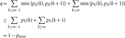 \begin{align*} q &=\sum _{k \leq m - 1}{\min{\{p_X(k),p_X(k+1)\}}} + \sum _{k \geq m}{\min{\{p_X(k),p_X(k+1)\}}} \\[5pt] &\leq \sum _{k \leq m-1}{p_X(k)} + \sum _{k \geq m}{p_X(k+1)} \\[5pt] &= 1 - p_{{\textrm{max}}}. \end{align*}
The bound 1 follows since
 $H(X) = \mathbb{E}\bigl ({\log{\frac{1}{p_X(X)}}\bigr )} \geq \log{\frac{1}{\max _k{p_X(k)}}}.$
For 2, note that since
 $p_X$
is unimodal,
$p_X$
is unimodal,
 ${p_X(k+1)} \geq{p_X(k)}$
for all
${p_X(k+1)} \geq{p_X(k)}$
for all
 $k \lt m$
and
$k \lt m$
and
 ${p_X(k+1)} \leq{p_X(k)}$
for all
${p_X(k+1)} \leq{p_X(k)}$
for all
 $k \geq m$
. Therefore, the inequality in part 1 is equality and 2 follows.
$k \geq m$
. Therefore, the inequality in part 1 is equality and 2 follows.
3. Proofs of Theorems 1 and 3
Let
 $U^{(n)} \;:\!=\; \sum _{i=1}^n{U_i},$
where
$U^{(n)} \;:\!=\; \sum _{i=1}^n{U_i},$
where
 $U_i$
are i.i.d. continuous uniforms on
$U_i$
are i.i.d. continuous uniforms on
 $(0,1).$
Let
$(0,1).$
Let
 $f_{S_n+U^{(n)}}$
denote the density of
$f_{S_n+U^{(n)}}$
denote the density of
 $S_n+U^{(n)}.$
We approximate
$S_n+U^{(n)}.$
We approximate
 $f_{S_n+U^{(n)}}$
with the p.m.f., say
$f_{S_n+U^{(n)}}$
with the p.m.f., say
 $p_{S_n}$
, of
$p_{S_n}$
, of
 $S_n$
.
$S_n$
.
We recall that the class of discrete log-concave distributions is closed under convolution [Reference Hoggar10] and hence the following lemma may be applied to
 $S_n$
.
$S_n$
.
Lemma 8.
Let
 $S$
be a log-concave random variable on the integers with variance
$S$
be a log-concave random variable on the integers with variance
 $\sigma ^2 = \textrm{Var}{(S)}$
and, for any
$\sigma ^2 = \textrm{Var}{(S)}$
and, for any
 $n \geq 1,$
denote by
$n \geq 1,$
denote by
 $f_{S+U^{(n)}}$
the density of
$f_{S+U^{(n)}}$
the density of
 $S + U^{(n)}$
on the real line. Then for any
$S + U^{(n)}$
on the real line. Then for any
 $n \geq 1$
and
$n \geq 1$
and
 $x \in \mathbb{R}$
,
$x \in \mathbb{R}$
,
 \begin{equation} f_{S+U^{(n)}}(x) = p_{S}(\lfloor x \rfloor ) + g_n(\lfloor x \rfloor,x), \end{equation}
for some
 $g_n\;:\;\mathbb{Z}\times \mathbb{R} \to \mathbb{R}$
satisfying
$g_n\;:\;\mathbb{Z}\times \mathbb{R} \to \mathbb{R}$
satisfying
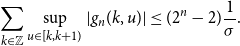 \begin{equation} \sum _{{k} \in \mathbb{Z}}\sup _{u\in [k,k+1)}{|g_n(k,u)|}\leq (2^{n} -2)\frac{1}{\sigma }. \end{equation}
Moreover, if
 $\lfloor x \rfloor \geq N_{\textrm{max}} + n - 1,$
 \begin{equation} f_{S+U^{(n)}}(x) \leq 2^np_{S}(\lfloor x \rfloor -n+1). \end{equation}
Proof. First we recall that for a discrete random variable
 $S$
and a continuous independent random variable
$S$
and a continuous independent random variable
 $U$
with density
$U$
with density
 $f_U$
,
$f_U$
,
 $S+U$
is continuous with density
$S+U$
is continuous with density
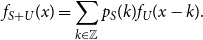 \begin{equation*} f_{S+U}(x) = \sum _{k \in \mathbb {Z}}{p_S(k)f_U(x-k)}. \end{equation*}
For
 $n=1$
, the statement is true with
$n=1$
, the statement is true with
 $g_n = 0$
. We proceed by induction on
$g_n = 0$
. We proceed by induction on
 $n$
with
$n$
with
 $n=2$
as base case, which illustrates the idea better. The density of
$n=2$
as base case, which illustrates the idea better. The density of
 $U_1+U_2$
is
$U_1+U_2$
is
 $f_{U_1+U_2}(u) = u,$
for
$f_{U_1+U_2}(u) = u,$
for
 $u\in (0,1)$
and
$u\in (0,1)$
and
 $f_{U_1+U_2}(u) = 2-u$
, for
$f_{U_1+U_2}(u) = 2-u$
, for
 $u \in [1,2)$
. Thus, we have
$u \in [1,2)$
. Thus, we have
 \begin{equation} f_{S+U^{(2)}}(x) = p_{S}(\lfloor x \rfloor ) + (1-x+\lfloor x \rfloor )(p_{S}(\lfloor x \rfloor -1) - p_{S}(\lfloor x \rfloor )). \end{equation}
Therefore,
 \begin{equation*} f_{S+U^{(2)}}(x) = p_{S}(\lfloor x \rfloor ) + g_2(\lfloor x \rfloor,x), \end{equation*}
where
 $g_2(k,x) = (1-x+{k})(p_{S}(k-1) - p_{S}(k))$
and by Propositions 4, 7.2 and Lemma 5
$g_2(k,x) = (1-x+{k})(p_{S}(k-1) - p_{S}(k))$
and by Propositions 4, 7.2 and Lemma 5
 \begin{equation*} \sum _{{k} \in \mathbb {Z}}\sup _{u\in [k,k+1)}|g_2(k,u)| \leq \sum _{k \in \mathbb {Z}}{|p_S(k) - p_S(k-1)|} = \|p_{S} - p_{S+1}\|_{1} \leq \frac {2}{\sigma }. \end{equation*}
Next, we have
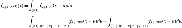 \begin{align} \nonumber f_{S+U^{(n+1)}}(x) &= \int _{(0,1)}{f_{S+U^{(n)}}(x-u)du} \\[5pt] &= \int _{(0,1)\cap (x-\lfloor x \rfloor -1,x-\lfloor x \rfloor )}{f_{S+U^{(n)}}(x-u)du} + \int _{(0,1)\cap (x-\lfloor x \rfloor,x-\lfloor x \rfloor +1)}{f_{S+U^{(n)}}(x-u)du}. \end{align}
Using the inductive hypothesis, (24) is equal to
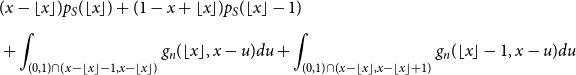 \begin{align} \nonumber &(x-\lfloor x \rfloor ) p_S(\lfloor x \rfloor ) + (1-x+\lfloor x \rfloor ) p_S(\lfloor x \rfloor -1) \\[5pt] &+ \int _{(0,1)\cap (x-\lfloor x \rfloor -1,x-\lfloor x \rfloor )}{g_{n}(\lfloor x \rfloor,x-u)du} + \int _{(0,1)\cap (x-\lfloor x \rfloor,x-\lfloor x \rfloor +1)}{g_n(\lfloor x \rfloor -1,x-u)du} \end{align}
with
 $g_n$
satisfying (21). Thus, we can write
$g_n$
satisfying (21). Thus, we can write
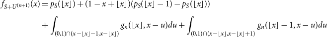 \begin{align} \nonumber f_{S+U^{(n+1)}}(x) & = p_S(\lfloor x \rfloor ) + (1-x+\lfloor x \rfloor )(p_S(\lfloor x \rfloor -1) - p_S(\lfloor x \rfloor )) \\[5pt] &+ \int _{(0,1)\cap (x-\lfloor x \rfloor -1,x-\lfloor x \rfloor )}{g_{n}(\lfloor x \rfloor,x-u)du} + \int _{(0,1)\cap (x-\lfloor x \rfloor,x-\lfloor x \rfloor +1)}{g_n(\lfloor x \rfloor -1,x-u)du} \end{align}
 \begin{align} &= p_S(\lfloor x \rfloor ) +g_{n+1}(\lfloor x \rfloor,x), \end{align}
where
 $g_{n+1}(k,x) =(1-x+k)(p_S(k-1) - p_S(k))+ \int _{(0,1)\cap (x-k-1,x-k)}{g_{n}(k,x-u)du}+$
 $ \int _{(0,1)\cap (x-k,x-k+1)}{g_n(k-1,x-u)du}$
. Therefore, since
$ \int _{(0,1)\cap (x-k,x-k+1)}{g_n(k-1,x-u)du}$
. Therefore, since
 $g_n$
satisfies (21),
$g_n$
satisfies (21),
 \begin{equation} \sum _{{k} \in \mathbb{Z}}\sup _{u\in [k,k+1)}|g_{n+1}({k},u)| \leq \frac{2}{\sigma } + 2\sum _{k \in \mathbb{Z}}{\sup _{u\in [k,k+1)}|g_{n}({k},u)|} \leq \frac{2}{\sigma } + 2(2^{n} -2)\frac{1}{\sigma } = (2^{n+1} - 2)\frac{1}{\sigma }, \end{equation}
completing the inductive step and thus the proof of (21).
Inequality (22) may be proved in a similar way by induction: For
 $n=2$
, by (23)
$n=2$
, by (23)
 \begin{equation} f_{S+U^{(2)}}(x) \leq 2p_S(\lfloor x \rfloor -1), \end{equation}
since
 $p_S(\lfloor x \rfloor ) \leq p_S(\lfloor x \rfloor -1)$
for
$p_S(\lfloor x \rfloor ) \leq p_S(\lfloor x \rfloor -1)$
for
 $\lfloor x \rfloor \geq N_{\textrm{max}}+1.$
By (24) and the inductive hypothesis
 \begin{align} f_{S+U^{(n+1)}}(x) &= \int _{(0,1)\cap (x-\lfloor x \rfloor -1,x-\lfloor x \rfloor )}{f_{S+U^{(n)}}(x-u)du} + \int _{(0,1)\cap (x-\lfloor x \rfloor,x-\lfloor x \rfloor +1)}{f_{S+U^{(n)}}(x-u)du} \end{align}
 \begin{align} &\leq 2^n p_S(\lfloor x \rfloor - n) + 2^np_S(\lfloor x \rfloor -n+1) \end{align}
 \begin{align} &\leq 2^{n+1}p_S(\lfloor x \rfloor -n) \end{align}
completing the proof of (22) and thus the proof of the lemma.
Lemma 9.
Let
 $X$
be a log-concave random variable on the integers with p.m.f.
$X$
be a log-concave random variable on the integers with p.m.f.
 $p$
, mean zero and variance
$p$
, mean zero and variance
 $\sigma ^2,$
and let
$\sigma ^2,$
and let
 $0\lt \epsilon \lt 1/2$
. If
$0\lt \epsilon \lt 1/2$
. If
 $\sigma \geq \max{\{3^{1/\epsilon },(12e^3)^{1/(1-2\epsilon )}\}},$
there is an
$\sigma \geq \max{\{3^{1/\epsilon },(12e^3)^{1/(1-2\epsilon )}\}},$
there is an
 $N_0 \in \{N_{\textrm{max}},\ldots,N_{\textrm{max}}+2\lceil \sigma ^2\rceil \}$
such that, for each
$N_0 \in \{N_{\textrm{max}},\ldots,N_{\textrm{max}}+2\lceil \sigma ^2\rceil \}$
such that, for each
 $k \geq N_0,$
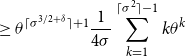
 \begin{equation} p(k+1) \leq \biggl (1-\frac{1}{\sigma ^{2-\epsilon }}\biggr ) p(k). \end{equation}
Similarly, there is an
 $N_0^- \in \{N_{\textrm{max}}-2\lceil \sigma ^2\rceil,\ldots,N_{\textrm{max}}\}$
such that, for each
$N_0^- \in \{N_{\textrm{max}}-2\lceil \sigma ^2\rceil,\ldots,N_{\textrm{max}}\}$
such that, for each
 $k \leq N_0^-,$
 \begin{equation*}p(k-1) \leq \biggl (1-\frac {1}{\sigma ^{2-\epsilon }}\biggr ) p(k).\end{equation*}
Proof. Let
 $\theta = 1-\frac{1}{\sigma ^{2-\epsilon }}.$
It suffices to show that there is an
$\theta = 1-\frac{1}{\sigma ^{2-\epsilon }}.$
It suffices to show that there is an
 $N_0 \in \{N_{\textrm{max}},\ldots,N_{\textrm{max}}+2\lceil \sigma ^2\rceil \}$
such that
$N_0 \in \{N_{\textrm{max}},\ldots,N_{\textrm{max}}+2\lceil \sigma ^2\rceil \}$
such that
 $p(N_0+1) \leq \theta p(N_0),$
since then, for each
$p(N_0+1) \leq \theta p(N_0),$
since then, for each
 $k \geq N_0, \frac{p(k+1)}{p(k)} \leq \frac{p(N_0+1)}{p(N_0)} \leq \theta$
by log-concavity.
$k \geq N_0, \frac{p(k+1)}{p(k)} \leq \frac{p(N_0+1)}{p(N_0)} \leq \theta$
by log-concavity.
Suppose for contradiction that
 $p(k+1) \geq \theta p(k)$
for each
$p(k+1) \geq \theta p(k)$
for each
 $ k \in \{N_{\textrm{max}},\ldots,N_{\textrm{max}}+2\lceil \sigma ^2\rceil \}$
. Then, we have, using (18)
$ k \in \{N_{\textrm{max}},\ldots,N_{\textrm{max}}+2\lceil \sigma ^2\rceil \}$
. Then, we have, using (18)
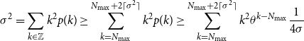 \begin{align} \sigma ^2 &= \sum _{k \in \mathbb{Z}}{k^2p(k)} \geq \sum _{k = N_{\textrm{max}}}^{N_{\textrm{max}}+2\lceil \sigma ^2\rceil }{k^2p(k)} \geq \sum _{k = N_{\textrm{max}}}^{N_{\textrm{max}}+2\lceil \sigma ^2\rceil }{k^2\theta ^{k-N_{\textrm{max}}}\frac{1}{4\sigma }} \end{align}
 \begin{align} &= \sum _{m=0}^{2\lceil \sigma ^2\rceil }(N_{\textrm{max}}+m)^2\theta ^m\frac{1}{4\sigma } \geq \sum _{m=\max \{0,-N_{\textrm{max}}\}}^{2\lceil \sigma ^2\rceil }(N_{\textrm{max}}+m)^2\theta ^m\frac{1}{4\sigma }. \end{align}
Now we use Proposition 6 with
 $\delta \gt 0$
to be chosen later. Thus, the right-hand side of (35) is at least
$\delta \gt 0$
to be chosen later. Thus, the right-hand side of (35) is at least
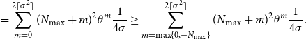
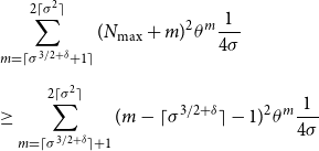 \begin{align} \nonumber &\sum _{m=\lceil \sigma ^{3/2+\delta }+1\rceil }^{2\lceil \sigma ^2\rceil }(N_{\textrm{max}}+m)^2\theta ^m\frac{1}{4\sigma } \\[5pt] &\geq \sum _{m=\lceil \sigma ^{3/2+\delta }\rceil +1}^{2\lceil \sigma ^2\rceil }(m - \lceil \sigma ^{3/2+\delta }\rceil -1)^2\theta ^m\frac{1}{4\sigma } \end{align}
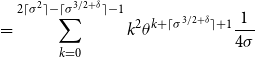 \begin{align} &= \sum _{k=0}^{2\lceil \sigma ^2\rceil - \lceil \sigma ^{3/2+\delta }\rceil -1}k^2\theta ^{k+\lceil \sigma ^{3/2+\delta }\rceil +1}\frac{1}{4\sigma } \end{align}
 \begin{align} &\geq \theta ^{\lceil \sigma ^{3/2+\delta }\rceil +1}\frac{1}{4\sigma }\sum _{k=1}^{\lceil \sigma ^2\rceil -1 }k\theta ^{k} \end{align}
 \begin{align} &= \frac{\theta ^{\lceil \sigma ^{3/2+\delta }\rceil +1}}{4\sigma }\left [\theta \frac{1-\theta ^{\lceil \sigma ^2\rceil }}{(1-\theta )^2} - \lceil \sigma ^2\rceil \frac{\theta ^{\lceil \sigma ^2\rceil }}{(1-\theta )} \right ]. \end{align}
Using the elementary bound
 $(1-x)^y \geq e^{-2xy},$
for
$(1-x)^y \geq e^{-2xy},$
for
 $0\lt x \lt \frac{\log{2}}{2},y\gt 0$
, we see that
$0\lt x \lt \frac{\log{2}}{2},y\gt 0$
, we see that
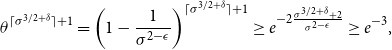 \begin{equation*} \theta ^{\lceil \sigma ^{3/2+\delta }\rceil +1} = \left(1-\frac {1}{\sigma ^{2-\epsilon }}\right)^{\lceil \sigma ^{3/2+\delta }\rceil +1} \geq e^{-2\frac {\sigma ^{3/2+\delta }+2}{\sigma ^{2-\epsilon }}} \geq e^{-3}, \end{equation*}
where the last inequality holds as long as
 $\epsilon +\delta \lt 1/2.$
Choosing
$\epsilon +\delta \lt 1/2.$
Choosing
 $\delta = 1/4-\epsilon/2,$
we see that the assumption of Proposition 6 is satisfied for
$\delta = 1/4-\epsilon/2,$
we see that the assumption of Proposition 6 is satisfied for
 $\sigma \gt 16^{1/(1-2\epsilon )}$
and thus for
$\sigma \gt 16^{1/(1-2\epsilon )}$
and thus for
 $\sigma \gt (12e^3)^{1/(1-2\epsilon )}$
as well. Furthermore, using
$\sigma \gt (12e^3)^{1/(1-2\epsilon )}$
as well. Furthermore, using
 $(1-x)^y \leq e^{-xy}, 0\lt x\lt 1, y \gt 0,$
we get
$(1-x)^y \leq e^{-xy}, 0\lt x\lt 1, y \gt 0,$
we get
 $\theta ^{\sigma ^2} \leq e^{-\sigma ^{\epsilon }}.$
Thus, the right-hand side of (39) is at least
$\theta ^{\sigma ^2} \leq e^{-\sigma ^{\epsilon }}.$
Thus, the right-hand side of (39) is at least
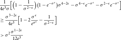 \begin{align} \nonumber &\frac{1}{4e^3\sigma }\Bigl [\Bigl (1-\frac{1}{\sigma ^{2-\epsilon }}\Bigr ) \bigl (1-e^{-\sigma ^{\epsilon }}\bigr )\sigma ^{4-2\epsilon } - \sigma ^{4-\epsilon }e^{-\sigma ^{\epsilon }} - \sigma ^{2-\epsilon }e^{-\sigma ^{\epsilon }}\Bigr ] \nonumber\\[5pt] &\geq \frac{\sigma ^{3-2\epsilon }}{4e^3}\Bigl [1-2\frac{\sigma ^{\epsilon }}{e^{\sigma ^\epsilon }} -\frac{1}{\sigma ^{2-\epsilon }}\Bigr ]\nonumber\\[5pt] &\gt \sigma ^2\frac{\sigma ^{1-2\epsilon }}{12e^3} \end{align}
 \begin{align} &\geq \sigma ^2, \end{align}
where (40) holds for
 $\sigma \gt 3^{\frac{1}{\epsilon }}$
, since then
$\sigma \gt 3^{\frac{1}{\epsilon }}$
, since then
 $\frac{\sigma ^{\epsilon }}{e^{\sigma ^{\epsilon }}} \leq \frac{1}{4}$
and
$\frac{\sigma ^{\epsilon }}{e^{\sigma ^{\epsilon }}} \leq \frac{1}{4}$
and
 $\sigma ^{-2+\epsilon } \lt \sigma ^{-1} \lt \frac{1}{9}$
. Finally, (41) holds for
$\sigma ^{-2+\epsilon } \lt \sigma ^{-1} \lt \frac{1}{9}$
. Finally, (41) holds for
 $\sigma \gt (12e^3)^{\frac{1}{1-2\epsilon }},$
getting the desired contradiction.
$\sigma \gt (12e^3)^{\frac{1}{1-2\epsilon }},$
getting the desired contradiction.
For the second part, apply the first part to the log-concave random variable
 $-X$
.
$-X$
.
Remark 10. The bound (33) may be improved due to the suboptimal step (38), e.g. by means of the identity
 \begin{equation*} \sum _{k=1}^M{k^2\theta ^k} = \theta \frac {{d}}{d\theta }\biggl (\sum _{k=1}^M{k\theta ^k}\biggr ) = \theta \frac {{d}}{d\theta } \Biggl (\theta \frac {{d}}{d\theta }\biggl (\sum _{k=1}^M{\theta ^k}\biggr ) \Biggr ) = \theta \frac {{d}}{d\theta } \Biggl (\theta \frac {{d}}{d\theta }\biggl (\frac {\theta -\theta ^{M+1}}{1-\theta }\biggr ) \Biggr ). \end{equation*}
It is, however, sufficient for our purpose as it will only affect a higher-order term in the proof of Theorem 1.
We are now ready to give the proof of Theorem 1 and of our main result, Theorem 3.
Proof of Theorem
1. Assume without loss of generality that
 $X_1$
has zero mean. Let
$X_1$
has zero mean. Let
 $F(x) = x\log{\frac{1}{x}}, x\gt 0$
and note that
$F(x) = x\log{\frac{1}{x}}, x\gt 0$
and note that
 $F(x)$
is non-decreasing for
$F(x)$
is non-decreasing for
 $x \leq 1/e$
. As before denote
$x \leq 1/e$
. As before denote
 $S_n = \sum _{i=1}^n{X_i},$
 $U^{(n)} = \sum _{i=1}^n{U_i}$
and let
$U^{(n)} = \sum _{i=1}^n{U_i}$
and let
 $f_{S_n+U^{(n)}}$
be the density of
$f_{S_n+U^{(n)}}$
be the density of
 $S_n+U^{(n)}$
on the reals. We have
$S_n+U^{(n)}$
on the reals. We have
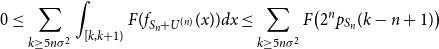
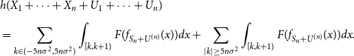 \begin{align} \nonumber &h(X_1+\cdots +X_n+U_1+\cdots +U_n)\\[5pt] &= \sum _{k \in (-5n\sigma ^2,5n\sigma ^2)}{\int _{[k,k+1)}{F(f_{S_n+U^{(n)}}(x)) dx}} + \sum _{|k| \geq 5n\sigma ^2}{\int _{[k,k+1)}{F(f_{S_n+U^{(n)}}(x)) dx}}. \end{align}
First, we will show that the “entropy tails”, i.e. the second term in (42), vanish as
 $\sigma ^2$
grows large. To this end, note that for
$\sigma ^2$
grows large. To this end, note that for
 $k \geq 5n\sigma ^2,$
we have
$k \geq 5n\sigma ^2,$
we have
 $p_{S_n}(k+1) \leq p_{S_n}(k),$
since by Proposition 6 applied to the log-concave random variable
$p_{S_n}(k+1) \leq p_{S_n}(k),$
since by Proposition 6 applied to the log-concave random variable
 $S_n$
,
$S_n$
,
 $N_{\textrm{max}} \leq n\sigma ^2+1$
as long as
$N_{\textrm{max}} \leq n\sigma ^2+1$
as long as
 $\sqrt{n}\sigma \gt 4$
. Thus, by (22), for
$\sqrt{n}\sigma \gt 4$
. Thus, by (22), for
 $k\geq 5n\sigma ^2$
and
$k\geq 5n\sigma ^2$
and
 $x \in [k,k+1),$
 $f_{S_n+U^{(n)}}(x) \leq 2^n{p}_{S_n}(k-n+1)$
. Hence, for
$f_{S_n+U^{(n)}}(x) \leq 2^n{p}_{S_n}(k-n+1)$
. Hence, for
 \begin{equation} \sigma \gt \frac{2^{n}}{\sqrt{n}}e, \end{equation}
we have, using the monotonicity of
 $F$
for
$F$
for
 $x\leq \frac{1}{e}$
,
$x\leq \frac{1}{e}$
,
 \begin{align} 0 &\leq \sum _{k \geq 5n\sigma ^2}{\int _{[k,k+1)}{F(f_{S_n+U^{(n)}}(x)) dx}} \leq \sum _{k \geq 5n\sigma ^2}{F\bigl (2^n p_{S_n}(k-n+1)\bigr ) } \end{align}
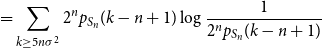 \begin{align} &= \sum _{k \geq 5n\sigma ^2}{2^np_{S_n}(k-n+1)\log{\frac{1}{2^np_{S_n}(k-n+1)}}} \end{align}
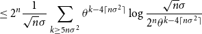 \begin{align} &\leq 2^n\frac{1}{\sqrt{n}\sigma } \sum _{k \geq 5n\sigma ^2}{\theta ^{k-4\lceil n\sigma ^2 \rceil }\log{\frac{\sqrt{n}\sigma }{2^n\theta ^{k-4\lceil n\sigma ^2 \rceil }}}} \end{align}
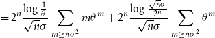 \begin{align} &= 2^n\frac{\log{\frac{1}{\theta }}}{\sqrt{n}\sigma } \sum _{m \geq n\sigma ^2}{m\theta ^{m}} + 2^n\frac{\log{\frac{\sqrt{n}\sigma }{2^n}}}{\sqrt{n}\sigma } \sum _{m \geq n\sigma ^2}{\theta ^{m}} \end{align}
 \begin{align} &\leq 2^{n+1} \frac{\log{\sqrt{n}\sigma }}{\sqrt{n}\sigma } \Bigl [ \frac{\theta ^{\lceil n\sigma ^2 \rceil +1}}{(1-\theta )^2} +\lceil n\sigma ^2 \rceil \frac{\theta ^{\lceil n\sigma ^2 \rceil }}{1-\theta } +\frac{\theta ^{\lceil n\sigma ^2 \rceil }}{1-\theta } \Bigr ] \end{align}
 \begin{align} &\leq 2^{n+1} \frac{\log{\sqrt{n}\sigma }}{\sqrt{n}\sigma }e^{-(\sqrt{n}\sigma )^{\epsilon }} \Bigl [ (\sqrt{n}\sigma )^{4-2\epsilon } + (n\sigma ^2+1)(\sqrt{n}\sigma )^{2-\epsilon } + (\sqrt{n}\sigma )^{2-\epsilon } \Bigr ] \end{align}
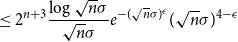 \begin{align} &\leq 2^{n+3} \frac{\log{\sqrt{n}\sigma }}{\sqrt{n}\sigma }e^{-(\sqrt{n}\sigma )^{\epsilon }} (\sqrt{n}\sigma )^{4-\epsilon } \end{align}
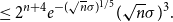 \begin{align} &\leq 2^{n+4} e^{-(\sqrt{n}\sigma )^{1/5}} (\sqrt{n}\sigma )^{3}. \end{align}
Here, (46) holds for
 \begin{equation} \sqrt{n}\sigma \gt 3^7 \end{equation}
with
 $\theta = 1-\frac{1}{(\sqrt{n}\sigma )^{2-\epsilon }}=1-\frac{1}{(\sqrt{n}\sigma )^{9/5}}$
, where we have used Lemma 9 with
$\theta = 1-\frac{1}{(\sqrt{n}\sigma )^{2-\epsilon }}=1-\frac{1}{(\sqrt{n}\sigma )^{9/5}}$
, where we have used Lemma 9 with
 $\epsilon = 1/5$
(which makes the assumption approximately minimal). In particular, repeated application of (33) yields
$\epsilon = 1/5$
(which makes the assumption approximately minimal). In particular, repeated application of (33) yields
 $p_{S_n}(k-n+1) \leq \theta ^{k-4\lceil n\sigma ^2 \rceil }p_{S_n}\bigl (4\lceil n\sigma ^2 \rceil -n+1\bigr ) \leq \frac{\theta ^{k-4\lceil n\sigma ^2 \rceil }}{\sqrt{n}\sigma }.$
We bound the left tail in the exact the same way, using the second part of Lemma 9:
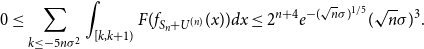 \begin{equation} 0 \leq \sum _{k \leq -5n\sigma ^2}{\int _{[k,k+1)}{F(f_{S_n+U^{(n)}}(x)) dx}} \leq 2^{n+4} e^{-(\sqrt{n}\sigma )^{1/5}} (\sqrt{n}\sigma )^{3}. \end{equation}
Next we will show that the first term in (42) is approximately
 $H(S_n)$
to complete the proof. We have
$H(S_n)$
to complete the proof. We have
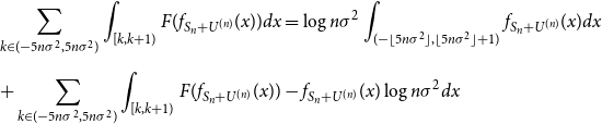 \begin{align} &\sum _{k \in (-5n\sigma ^2,5n\sigma ^2)}{\int _{[k,k+1)}{F(f_{S_n+U^{(n)}}(x)) dx}} = \log{n\sigma ^2}\int _{(-\lfloor 5n\sigma ^2\rfloor,\lfloor 5n\sigma ^2 \rfloor +1)}{f_{S_n+U^{(n)}}(x)dx} \nonumber \\[5pt] &+ \sum _{k \in (-5n\sigma ^2,5n\sigma ^2)}{\int _{[k,k+1)}{F(f_{S_n+U^{(n)}}(x)) - f_{S_n+U^{(n)}}(x)\log{n\sigma ^2}dx}} \end{align}
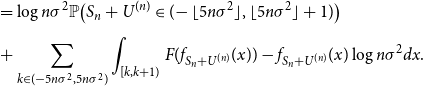 \begin{align} &= \log{n\sigma ^2}\mathbb{P}\bigl (S_n+U^{(n)} \in (\!-\lfloor 5n\sigma ^2 \rfloor,\lfloor 5n\sigma ^2 \rfloor +1)\bigr ) \nonumber \\[5pt] &+ \sum _{k \in (-5n\sigma ^2,5n\sigma ^2)}{\int _{[k,k+1)}{F(f_{S_n+U^{(n)}}(x)) - f_{S_n+U^{(n)}}(x)\log{n\sigma ^2}dx}}. \end{align}
Now we will apply the estimate of Lemma 12, which is stated and proved in the Appendix, to the integrand of the second term in (54) with
 $G(x) = F(x) - x\log{(n\sigma ^2)},$
 $\mu = \frac{1}{11\sigma \sqrt{n}}, D = 2^n\sqrt{n}\sigma, M = n\sigma ^2, a = f_{S_n+U^{(n)}}(x)$
and
$\mu = \frac{1}{11\sigma \sqrt{n}}, D = 2^n\sqrt{n}\sigma, M = n\sigma ^2, a = f_{S_n+U^{(n)}}(x)$
and
 $b=p_{S_n}(k).$
We obtain, using Lemma 8,
$b=p_{S_n}(k).$
We obtain, using Lemma 8,
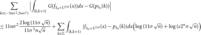 \begin{align} & \sum _{k \in (-5n\sigma ^2,5n\sigma ^2)}{\Bigl |\int _{[k,k+1)}{G(f_{S_n+U^{(n)}}(x))dx}} -{G(p_{S_n}(k))} \Bigr | \nonumber \\[5pt] &\leq 11n\sigma ^2\frac{2\log{(11\sigma \sqrt{n})}}{11\sigma ^3n\sqrt{n}} + \sum _{k \in \mathbb{Z}}{\int _{[k,k+1)}|f_{S_n+U^{(n)}}(x) - p_{S_n}(k)|dx}\Bigl (\log{(11\sigma \sqrt{n})} + \log (e2^n\sigma \sqrt{n})\Bigr ) \end{align}
 \begin{align} & \leq \frac{2\log{(11\sigma \sqrt{n})}}{\sigma \sqrt{n}} + \sum _{k\in \mathbb{Z}}{\sup _{x \in [k,k+1)}|g_n(k, x)|}\Bigl (\log{(11\sigma \sqrt{n})} + \log (e2^n\sigma \sqrt{n})\Bigr ) \end{align}
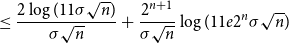 \begin{align} &\leq \frac{2\log{(11\sigma \sqrt{n})}}{\sigma \sqrt{n}} + \frac{2^{n+1}}{\sigma \sqrt{n}}\log (11e2^n\sigma \sqrt{n}) \end{align}
 \begin{align} &\leq \frac{3}{4}\frac{2^{n+2}}{\sigma \sqrt{n}}\log (11e2^{n}\sigma \sqrt{n}) \end{align}
 \begin{align} &\leq \frac{2^{n+2}}{\sigma \sqrt{n}}\log ((11e)^{3/4}2^{n}\sigma ^{3/4}\sqrt{n}) \leq \frac{2^{n+2}}{\sigma \sqrt{n}}\log (2^{n+2}\sigma \sqrt{n}), \end{align}
where
 $g_n(k,x)$
is given by Lemma 8 applied to the log-concave random variable
$g_n(k,x)$
is given by Lemma 8 applied to the log-concave random variable
 $S_n$
and therefore
$S_n$
and therefore
 $\sum _k{\sup _{x \in [k,k+1)}g_n(k, x)} \leq \frac{2^n}{\sigma \sqrt{n}}.$
In the last inequality in (60) we have used that
$\sum _k{\sup _{x \in [k,k+1)}g_n(k, x)} \leq \frac{2^n}{\sigma \sqrt{n}}.$
In the last inequality in (60) we have used that
 $\frac{(11e)^{3/4}}{\sigma ^{1/4}} \leq 4,$
for
$\frac{(11e)^{3/4}}{\sigma ^{1/4}} \leq 4,$
for
 $\sigma \gt 3^7$
. Therefore, by (54) and (60),
$\sigma \gt 3^7$
. Therefore, by (54) and (60),
 \begin{align} \nonumber &\Bigl | H(S_n) - \sum _{k \in (-5n\sigma ^2,5n\sigma ^2)}{\int _{[k,k+1)}{F(f_{S_n+U^{(n)}}(x)) dx}} \Bigr | \\[5pt] \nonumber &\leq \Bigl | H(S_n) -\sum _{k \in (-5n\sigma ^2,5n\sigma ^2)}{G(p_{S_n}(k))} - \log{n\sigma ^2}\mathbb{P}\bigl (S_n+U^{(n)} \in (\!-\lfloor 5n\sigma ^2 \rfloor,\lfloor 5n\sigma ^2 \rfloor +1)\bigr ) \Bigr | \\[5pt] &+ \frac{2^{n+2}}{\sigma \sqrt{n}}\log (2^{n+2}\sigma \sqrt{n}) \end{align}
 \begin{align} \nonumber &\leq \Bigl | H(S_n) -\sum _{k \in (-5n\sigma ^2,5n\sigma ^2)}{F(p_{S_n}(k))}\Bigr | + \frac{2^{n+2}}{\sigma \sqrt{n}}\log (2^{n+2}\sigma \sqrt{n}) \\[5pt] & + \log{n\sigma ^2}\Bigl | \mathbb{P}\bigl (S_n+U^{(n)} \in (\!-\lfloor 5n\sigma ^2 \rfloor,\lfloor 5n\sigma ^2 \rfloor +1)\bigr ) - \mathbb{P}\bigl (S_n\in (\!-5n\sigma ^2,5n\sigma ^2+ 1)\bigr )\Bigr | \\[5pt] \nonumber &\leq \sum _{|k| \geq 5n\sigma ^2}{F(p_{S_n}(k))} + \frac{2^{n+2}}{\sigma \sqrt{n}}\log (2^{n+2}\sigma \sqrt{n}) \end{align}
 \begin{align} &+ \log{n\sigma ^2}\Bigl | \mathbb{P}\bigl (S_n+U^{(n)} \in (\!-\lfloor 5n\sigma ^2 \rfloor,\lfloor 5n\sigma ^2 \rfloor +1)\bigr ) - \mathbb{P}\bigl (S_n\in (\!-5n\sigma ^2,5n\sigma ^2+ 1)\bigr )\Bigr |. \end{align}
But, in view of (45), we can bound the discrete tails in the same way:
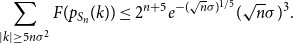 \begin{equation} \sum _{|k| \geq 5n\sigma ^2}{F(p_{S_n}(k))} \leq 2^{n+5} e^{-(\sqrt{n}\sigma )^{1/5}} (\sqrt{n}\sigma )^{3}. \end{equation}
Finally, note that by Chebyshev’s inequality
 \begin{align} 0\leq \mathbb{P}\bigl (S_n+U^{(n)} \notin (\!-\lfloor 5n\sigma ^2\rfloor,\lfloor 5n\sigma ^2\rfloor + 1)\bigr ) &\leq \mathbb{P}\left (|S_n+U^{(n)} - \frac{n}{2}| \gt 4n\sigma ^2\right ) \leq \frac{1}{8n\sigma ^2} \end{align}
and the same upper bound applies to
 $\mathbb{P}\bigl (S_n\notin (\!-\!5n\sigma ^2,5n\sigma ^2+ 1)\bigr )$
. Since both probabilities inside the absolute value in (63) are also upper bounded by
$\mathbb{P}\bigl (S_n\notin (\!-\!5n\sigma ^2,5n\sigma ^2+ 1)\bigr )$
. Since both probabilities inside the absolute value in (63) are also upper bounded by
 $1$
, replacing the bounds (65) and (66) into (63), we get
$1$
, replacing the bounds (65) and (66) into (63), we get
 \begin{align} \nonumber &\Bigl | H(S_n) - \sum _{k \in (-5n\sigma ^2,5n\sigma ^2)}{\int _{[k,k+1)}{F(f_{S_n+U^{(n)}}(x)) dx}} \Bigr | \\[5pt] &\leq 2^{n+5} e^{-(\sqrt{n}\sigma )^{1/5}} (\sqrt{n}\sigma )^{3} + \frac{2^{n+2}}{\sigma \sqrt{n}}\log (2^{n+2}\sigma \sqrt{n}) +\frac{\log{n\sigma ^2}}{8n\sigma ^2}. \end{align}
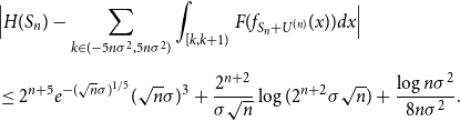
In view of (42) and the bounds on the continuous tails (51), (53), we conclude
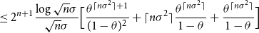
 \begin{align} \bigl |h(S_n+U^{(n)}) - H(S_n)\bigr | \leq 2^{n+6} e^{-(\sqrt{n}\sigma )^{1/5}} (\sqrt{n}\sigma )^{3} + \frac{2^{n+2}}{\sigma \sqrt{n}}\log (2^{n+2}\sigma \sqrt{n}) +\frac{\log{n\sigma ^2}}{8n\sigma ^2} \end{align}
as long as (43) and (52) are satisfied, that is as long as
 $\sigma \gt \max \{2^{n+2}/\sqrt{n},3^7/\sqrt{n}\}$
.
$\sigma \gt \max \{2^{n+2}/\sqrt{n},3^7/\sqrt{n}\}$
.
Remark 11. The exponent in (51) can be improved due to the suboptimal step (38) in Lemma 9. However, this is only a third-order term and therefore the rate in Theorem 1 would still be of the same order.
Proof of Theorem
3. Let
 $U_1,\ldots,U_n$
be continuous i.i.d. uniforms on
$U_1,\ldots,U_n$
be continuous i.i.d. uniforms on
 $(0,1).$
Then by the generalised EPI for continuous random variables [Reference Artstein, Ball, Barthe and Naor1, Reference Madiman and Barron11]
$(0,1).$
Then by the generalised EPI for continuous random variables [Reference Artstein, Ball, Barthe and Naor1, Reference Madiman and Barron11]
 \begin{equation} h\Bigl (\frac{X_1+\cdots +X_{n+1}+U_1+\cdots +U_{n+1}}{\sqrt{n+1}}\Bigr ) \geq h\Bigl (\frac{X_1+\cdots +X_{n}+U_1+\cdots +U_{n}}{\sqrt{n}}\Bigr ). \end{equation}
But by the scaling property of differential entropy [Reference Cover and Thomas4], this is equivalent to
 \begin{equation} h(X_1+\cdots +X_{n+1} + U_1+\cdots +U_{n+1}) \geq h(X_1+\cdots +X_{n} + U_1+\cdots +U_{n}) + \frac{1}{2}\log{\Bigl (\frac{n+1}{n}\Bigr )}. \end{equation}
Now we claim that for every
 $n\geq 1$
, if
$n\geq 1$
, if
 $H(X_1) \geq \log{\frac{2}{\epsilon }} + \log{\log{\frac{2}{\epsilon }}} + n + 26$
then
$H(X_1) \geq \log{\frac{2}{\epsilon }} + \log{\log{\frac{2}{\epsilon }}} + n + 26$
then
 \begin{equation} | h(X_1+\cdots +X_{n} + U_1+\cdots +U_{n}) - H(X_1+\cdots +X_{n})| \leq \frac{\epsilon }{2}. \end{equation}
Then the result follows from (71), applied to both sides of (70) (for
 $n$
and
$n$
and
 $n+1$
, respectively).
$n+1$
, respectively).
To prove the claim (71), we invoke Theorem 1. To this end let
 $n \geq 1$
and assume that
$n \geq 1$
and assume that
 $H(X_1) \geq \log{\frac{2}{\epsilon }} + \log{\log{\frac{2}{\epsilon }}} + n + 26$
. First we note, that since [Reference Cover and Thomas4]
$H(X_1) \geq \log{\frac{2}{\epsilon }} + \log{\log{\frac{2}{\epsilon }}} + n + 26$
. First we note, that since [Reference Cover and Thomas4]
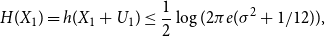 \begin{equation} H(X_1) = h(X_1 + U_1) \leq \frac{1}{2}\log{(2\pi e(\sigma ^2 +1/12))}, \end{equation}
we have
 $e^{H(X_1)} \leq 6\sigma$
provided that
$e^{H(X_1)} \leq 6\sigma$
provided that
 $\sigma \gt 0.275$
. Thus,
$\sigma \gt 0.275$
. Thus,
 $H(X_1) \geq 26$
implies
$H(X_1) \geq 26$
implies
 $\sigma \gt 50^6 \gt 90^5$
. Therefore the assumptions of the theorem are satisfied and we get
$\sigma \gt 50^6 \gt 90^5$
. Therefore the assumptions of the theorem are satisfied and we get
 \begin{align} \nonumber &| h(X_1+\cdots +X_{n} + U_1+\cdots +U_{n}) - H(X_1+\cdots +X_{n})| \\[5pt] &\leq 2^{n+6} e^{-(\sqrt{n}\sigma )^{1/5}} (\sqrt{n}\sigma )^{3} + \frac{2^{n+2}}{\sigma \sqrt{n}}\log (2^{n+2}\sigma \sqrt{n}) +\frac{\log{n\sigma ^2}}{8n\sigma ^2} \end{align}
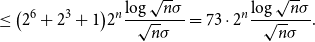 \begin{align} &\leq \bigl (2^6+2^3+1\bigr )2^{n}\frac{\log{\sqrt{n}\sigma }}{\sqrt{n}\sigma } = 73\cdot 2^n\frac{\log{\sqrt{n}\sigma }}{\sqrt{n}\sigma }. \end{align}
In (74), we used the elementary fact that for
 $x \geq 90^5$
,
$x \geq 90^5$
,
 $\frac{x^3}{e^{x^{1/5}}} \leq \frac{1}{x} \leq \frac{\log{x}}{x}$
to bound the first term and the assumption
$\frac{x^3}{e^{x^{1/5}}} \leq \frac{1}{x} \leq \frac{\log{x}}{x}$
to bound the first term and the assumption
 $\sigma \sqrt{n} \geq 2^{n+2}$
to bound the second term. Thus, by assumption
$\sigma \sqrt{n} \geq 2^{n+2}$
to bound the second term. Thus, by assumption
 $\sigma \geq \frac{e^{H(X_1)}}{6} \geq \frac{2}{\epsilon }\log{\frac{2}{\epsilon }}e^{n+24}$
and since
$\sigma \geq \frac{e^{H(X_1)}}{6} \geq \frac{2}{\epsilon }\log{\frac{2}{\epsilon }}e^{n+24}$
and since
 $ \frac{\log{x}}{x}$
is non-increasing for
$ \frac{\log{x}}{x}$
is non-increasing for
 $x \gt{e}$
, we obtain by (74)
$x \gt{e}$
, we obtain by (74)
 \begin{align} &| h(X_1+\cdots +X_{n} + U_1+\cdots +U_{n}) - H(X_1+\cdots +X_{n})| \end{align}
 \begin{align} &\leq 73\cdot 2^n\frac{\log{\frac{2}{\epsilon }} + \log{\log{\frac{2}{\epsilon }}} + n + 24}{\frac{2}{\epsilon }\log{\frac{2}{\epsilon }e^ne^{24}}} \end{align}
 \begin{align} &\leq \frac{\epsilon }{2}\Bigl [\frac{146}{(\frac{e}{2})^ne^{24}} + \frac{n73}{\log{\frac{2}{\epsilon }}(\frac{e}{2})^ne^{24}} + \frac{1752}{\log{\frac{2}{\epsilon }}(\frac{e}{2})^ne^{24}}\Bigr ] \end{align}
 \begin{align} &\lt \frac{\epsilon }{2} \end{align}
proving the claim (71) and thus the theorem.
Acknowledgements
The author is indebted to Ioannis Kontoyiannis for interesting discussions as well as many useful suggestions and comments. The author would also like to thank the two anonymous reviewers for the careful reading of the manuscript and for many useful comments that significantly improved the presentation of the results in the paper.
Appendix
An elementary Lemma
Here, we prove the following Taylor-type estimate that we used in the proof of Theorem 1. A similar estimate was used in [Reference Tao17].
Lemma 12.
Let
 $D, M \geq 1$
and, for
$D, M \geq 1$
and, for
 $x \gt 0,$
consider
$x \gt 0,$
consider
 $G(x) = F(x) -x\log{M}$
, where
$G(x) = F(x) -x\log{M}$
, where
 $F(x) = -x\log{x}.$
Then, for
$F(x) = -x\log{x}.$
Then, for
 $0 \leq a,b \leq \frac{D}{M}$
and any
$0 \leq a,b \leq \frac{D}{M}$
and any
 $0 \lt \mu \lt \frac{1}{e},$
we have the estimate
$0 \lt \mu \lt \frac{1}{e},$
we have the estimate
 \begin{equation} |G(b) - G(a)| \leq \frac{2\mu }{M}\log{\frac{1}{\mu }} + |b-a|\bigl [\log{\frac{1}{\mu }} + \log{(eD)}\bigr ]. \end{equation}
Proof. Note that
 ${G}^{\prime }(x) = -\log{x} - 1 - \log{M}$
, which is non-negative for
${G}^{\prime }(x) = -\log{x} - 1 - \log{M}$
, which is non-negative for
 $x \lt \frac{1}{eM}$
.
$x \lt \frac{1}{eM}$
.
We will consider two cases separately.
The first case is when either
 $a \lt \frac{\mu }{M}$
or
$a \lt \frac{\mu }{M}$
or
 $b \lt \frac{\mu }{M}$
. Assume without loss of generality that
$b \lt \frac{\mu }{M}$
. Assume without loss of generality that
 $a \lt \frac{\mu }{M}$
. Then if
$a \lt \frac{\mu }{M}$
. Then if
 $b \lt \frac{\mu }{M}$
as well, we have
$b \lt \frac{\mu }{M}$
as well, we have
 $|G(b) - G(a)| \leq G(a) + G(b) \leq \frac{2\mu }{M}\log{\frac{1}{\mu }},$
since then
$|G(b) - G(a)| \leq G(a) + G(b) \leq \frac{2\mu }{M}\log{\frac{1}{\mu }},$
since then
 ${G}^{\prime } \geq 0$
. On the other hand, if
${G}^{\prime } \geq 0$
. On the other hand, if
 $b \geq \frac{\mu }{M}\gt a$
then
$b \geq \frac{\mu }{M}\gt a$
then
 $G(a) \geq a\log{\frac{1}{\mu }}$
and
$G(a) \geq a\log{\frac{1}{\mu }}$
and
 $G(b) \leq b\log{\frac{1}{\mu }}$
.
$G(b) \leq b\log{\frac{1}{\mu }}$
.
But then, either
 $G(b) \gt G(a),$
whence
$G(b) \gt G(a),$
whence
 $|G(b) - G(a)| \leq |b-a|\log{\frac{1}{\mu }}$
or
$|G(b) - G(a)| \leq |b-a|\log{\frac{1}{\mu }}$
or
 $G(b) \lt G(a),$
whence
$G(b) \lt G(a),$
whence
 $|G(b)-G(a)| \leq |b-a|\log{(eD)},$
since we must have
$|G(b)-G(a)| \leq |b-a|\log{(eD)},$
since we must have
 $G(a) - G(b) = (a-b)G^{\prime }(\xi ),$
for some
$G(a) - G(b) = (a-b)G^{\prime }(\xi ),$
for some
 $\xi \in (\frac{1}{eM},\frac{D}{M}]$
.
$\xi \in (\frac{1}{eM},\frac{D}{M}]$
.
Thus, in the first case,
 $|G(b) - G(a)| \leq \frac{2\mu }{M}\log{\frac{1}{\mu }} + |b-a|\bigl [\log{\frac{1}{\mu }} + \log (eD)\bigr ]$
.
$|G(b) - G(a)| \leq \frac{2\mu }{M}\log{\frac{1}{\mu }} + |b-a|\bigl [\log{\frac{1}{\mu }} + \log (eD)\bigr ]$
.
The second case, is when both
 $a,b \geq \frac{\mu }{M}$
. Then
$a,b \geq \frac{\mu }{M}$
. Then
 $G(b) - G(a) = (b-a){G}^{\prime }(\xi )$
, for some
$G(b) - G(a) = (b-a){G}^{\prime }(\xi )$
, for some
 $\frac{D}{M} \geq \xi \geq \mu \frac{1}{M}$
.
$\frac{D}{M} \geq \xi \geq \mu \frac{1}{M}$
.
Since then
 $|{G}^{\prime }(\xi )| \leq \log{\frac{1}{\mu }} + \log{D}+1$
, we have
$|{G}^{\prime }(\xi )| \leq \log{\frac{1}{\mu }} + \log{D}+1$
, we have
 $|G(b) - G(a)| \leq |b-a|(\log{\frac{1}{\mu }} + \log{(eD)})$
.
$|G(b) - G(a)| \leq |b-a|(\log{\frac{1}{\mu }} + \log{(eD)})$
.
In any case,
 $|G(b) - G(a)| \leq \frac{2\mu }{M}\log{\frac{1}{\mu }} + |b-a|\bigl [\log{\frac{1}{\mu }} + \log{(eD)}\bigr ].$

