1 Introduction
It has been repeatedly argued that individuals make adaptive use of different decision strategies (Payne, Bettman, & Johnson, Reference Payne, Bettman and Johnson1993; Gigerenzer & Todd, Reference Gigerenzer and Todd1999) and that the application of the respective strategy might depend on different factors such as participants’ characteristics (e.g., intelligence; Bröder, Reference Bröder2003; Hilbig, Reference Hilbig2008), effort accuracy trade-offs (Payne, Bettman, & Johnson, Reference Payne, Bettman and Johnson1988), learning experiences (Rieskamp, Reference Rieskamp2006), presentation format (Glöckner & Betsch, Reference Glöckner and Betsch2008a; Bröder & Schiffer, Reference Bröder and Schiffer2003) and situational forces (e.g., time pressure, Payne et al., Reference Payne, Bettman and Johnson1988). Some strategies might be entirely based on deliberate computations (for an overview, see Payne et al., Reference Payne, Bettman and Johnson1988). Others, by contrast, might partially rely on automatic-intuitive processes (for an overview, see Glöckner & Witteman, Reference Glöckner and Witteman2010a). Glöckner and Betsch (Reference Glöckner and Betsch2008a) showed that classic process tracing methods such as Mouselab (Payne et al., Reference Payne, Bettman and Johnson1988) might hinder information search processes that are necessary for applying automatic processes. Furthermore, taking into account intuitive-automatic processes, many strategies make essentially the same choice predictions (i.e., weighted compensatory information integration; e.g., Brehmer, Reference Brehmer1994; Busemeyer & Townsend, Reference Busemeyer and Townsend1993; Busemeyer & Johnson, Reference Busemeyer and Johnson2004; Glöckner & Betsch, Reference Glöckner and Betsch2008b; see also Hammond, Hamm, Grassia, & Pearson, Reference Hammond, Hamm, Grassia and Pearson1987; Brunswik, Reference Brunswik1955). Glöckner (Reference Glöckner2009) showed that, considering strategies that make different choice predictions, people can be more efficiently classified by applying the Multiple-Measure Maximum Likelihood strategy classification method (MM-ML) as compared to relying on a choice-based strategy classification alone (Bröder & Schiffer, Reference Bröder and Schiffer2003; Bröder, Reference Bröder2010). Furthermore, the MM-ML method also allows us to differentiate between strategies that make the same choice predictions, given that decision time predictions aid discrimination.
Preparing an experiment to generate data for the application of the MM-ML method comprises three basic steps: (1) choose dependent measures (and specify the distributions of those measures), (2) choose a set of strategies, (3) select items that differentiate between the considered strategies and derive predictions on the dependent measures. Then the fit of the predictions of the strategies to individuals’ empirical data is calculated using MM-ML and the strategy most likely accounting for individuals’ behavior is identified. Glöckner (Reference Glöckner2009) provided an implementation of the MM-ML method in STATA – a commercial package for data analysis. To facilitate the access to the MM-ML method, we introduce the implementation of the MM-ML method in R – a non-commercial, publicly available, and open source package for data analysis.
2 Theory primer
In the following, we will present the key elements of the MM-ML method and introduce the variables used in Equation 1 (see below). For more details, see Glöckner (Reference Glöckner2009; Reference Glöckner2010).
2.1 Dependent measures
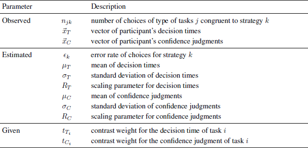
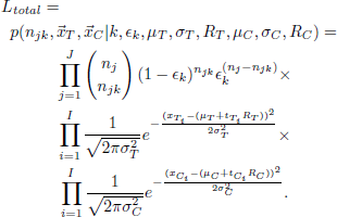
The default dependent measures analyzed in the MM-ML method are choices, decision times, and confidence judgments (Glöckner, Reference Glöckner2009). For choices, it is assumed that participants apply strategies with an equal error rate for all types of tasks/trials (see also Bröder & Schiffer, Reference Bröder and Schiffer2003; Bröder, Reference Bröder2010). Hence, the number of choices congruent with strategy predictions should be binomially distributed. Let k be the index number for strategies and j the index number for task types considered. The frequencies of decisions in line with the predictions of a strategy for each task type, njk , and the total number of tasks per type, nj , can then be used to estimate the error rate єk which maximizes the fit between predictions and individual choices (see first part of Equation 1).
For (log-transformed) decision times (T) and confidence judgments (C), we assume that each observation xT (xC) from the total vector of observations ![]() T (
T (![]() C) stems from a normal distribution with mean µTk=µT+tTiRT (µCk=µC+tCiRC) and variance σT 2 (σC 2). RT (RC) is a scaling parameter and tTi (tCi) is the prediction/contrast derived from strategy k (see next paragraph for details). The coefficients µT, σT, RT, µC, σC, and RC need to be estimated through maximum likelihood estimation. All variables are included in normal distribution functions that constitute part 2 and part 3 of Equation 1. Descriptions for all variables can be found in Table 1.
C) stems from a normal distribution with mean µTk=µT+tTiRT (µCk=µC+tCiRC) and variance σT 2 (σC 2). RT (RC) is a scaling parameter and tTi (tCi) is the prediction/contrast derived from strategy k (see next paragraph for details). The coefficients µT, σT, RT, µC, σC, and RC need to be estimated through maximum likelihood estimation. All variables are included in normal distribution functions that constitute part 2 and part 3 of Equation 1. Descriptions for all variables can be found in Table 1.
Table 1: Description of parameters of the likelihood function (see Equation 1)
The likelihood of a data vector for each strategy and participant can therefore be calculated by (Glöckner, Reference Glöckner2009, Equation 8, p. 191):
To take the number of free parameters into account in model evaluation, we compare the BIC values instead of the log-likelihoods for strategy classification. The BIC values can be calculated by (Glöckner, Reference Glöckner2009, Equation 9, p. 191): BIC=−2ln(Ltotal)+ln (Nobs)Np.
Ltotal is the likelihood of the data given the application of the respective strategy (Equation 1). Nobs is the number of task types times the number of dependent measures. Np is the number of the parameters that need to be estimated. If the strategy makes differentiated predictions for choices, decision times, and confidence over task types, overall seven parameters are estimated (єk, µT, σT, RT, µC, σC, and RC). For strategies that predict all equal decision times or confidence judgments (e.g., an equal-weights-rule in tasks in which the number of attributes per choice option is held constant), one parameter less is estimated (RT or RC omitted), respectively. For a strategy which assumes random choices (RANDOM), єk is omitted from estimation as well.
The MM-ML method is not limited to the measures discussed. Any measure (for further measures, see Payne et al., Reference Payne, Bettman and Johnson1988; Glöckner & Witteman, Reference Glöckner and Witteman2010b) can easily be added, as long as (1) the distribution of the measure is known and (2) predictions for the measure can be derived from each strategy, and thus contrasts can be formulated.
2.2 Strategies
The MM-ML method is not limited to a specific set of strategies; it is applicable to any set of strategies as long as predictions for the measures can be derived from the strategy. In the current example, we use five strategies. All but one (i.e., RANDOM) can be easily replaced by other strategies.
The default strategies we use in the MM-ML method are “Take The Best” (TTB), “Equal Weight” (EQW), “Weighted Additive Corrected” (WADDcorrected) (Payne et al., Reference Payne, Bettman and Johnson1993; Gigerenzer & Todd, Reference Gigerenzer and Todd1999; Glöckner & Betsch, Reference Glöckner and Betsch2008a), “Parallel Constraint Satisfaction” (PCS) (Glöckner, Reference Glöckner2006; Glöckner & Betsch, Reference Glöckner and Betsch2008b), and the “Random Model” (RANDOM), which is tantamount to guessing. Table 2 summarizes predictions of these strategies for six task types which are used for illustration. These tasks are probabilistic inferences in which decision makers choose which option is superior, based on dichotomous predictions of four different cues with certain predictive power (cue validity).
Table 2: Types of decision tasks and predictions of strategies
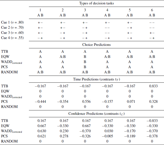
Note. In the upper part of the table, the item types are presented. The cue validities v are provided beside each cue. The cue values are “+” for “cue is present” and “−” for “cue is absent”. Below, the predictions for choices are shown. A and B stand for the predicted option. “A:B” indicates random choices between A and B. The lower part of the table shows predictions for decision times and confidences expressed in contrast weights that add up to zero and have a range of 1. Contrast values represent relative weights comparing different cue patterns for one strategy (modified after Glöckner, Reference Glöckner2009; Reference Glöckner2010).
For example, a participant strictly following TTB chooses option A for all tasks; for each type of task, the first cue that discriminates between options always points to option A.
Predictions of decision times are derived from the number of computational steps needed to apply the respective strategy (TTB, EQW, WADDcorrected) and the number of iterations necessary to find a consistent solution of the PCS network (Glöckner & Betsch, 2008b). Predictions of confidence judgments are based on differences between the weighted (WADDcorrected) and unweighted (EQW) sum of cues, the validity of the differentiating cue (TTB), and the difference of activation between options (PCS). Predictions are transformed into contrasts with a range of 1 and a sum of values of 0. For RANDOM, we expect strategy consistent choice behavior to be at chance level (fixed єk=0.5) and no differences in decision times and confidence judgments between the six types of decision tasks (thus RT and RC are set to 0).
The lower part of Table 2 shows the contrasts for decision times and confidence judgments for all strategies and six task types. For example, a participant strictly following TTB investigates only one cue for the first five types of task and three cues for the sixth type of task. Hence, more computational steps were necessary for applying TTB to the latter tasks. Specifically, 4 computational steps for the first five types of task (investigate cue 1 option A, investigate cue 1 option B, compare cues, choose option) and 10 computational steps for the sixth type of task, and therefore decision times should be longer (e.g., Bröder & Gaissmaier, Reference Bröder and Gaissmaier2007; Payne, Bettman, & Johnson, Reference Payne, Bettman and Johnson1988). Furthermore, a decision for option A is based on a cue with a validity of .80 for the first five types of task and a validity of .60 for the sixth type of task. For TTB, we use the validity of the cue on which the decision is based as an indicator of judgment confidence (Gigerenzer, Hoffrage, & Kleinbölting, Reference Gigerenzer, Hoffrage and Kleinbölting1991). In order finally to derive the contrast vectors for TTB displayed in Table 2, we rescaled the prediction vectors for decision time [4 4 4 4 4 10] and for judgment confidence [.8 .8 .8 .8 .8 .6] into vectors of a range of values of 1 and a sum of values of 0.
3 Implementation of the MM-ML method in R
R (Reference Team.2010) is software for statistical analysis under the GNU general public license, e.g., it is free of any charge. R is available for Windows, Mac, and UNIX systems. To download R, visit the “Comprehensive R Archive Network” (http://cran.r-project.org/). To learn more about R, we propose the free introduction to R by Paradis (Reference Paradis2005); however, to apply the MM-ML method in R, no sophisticated prior experience with the R syntax is required. In this paper, we provide two different implementations of MM-ML in R.Footnote 1 First, we describe a detailed implementation of MM-ML as syntax code that is similar to the implementation in STATA described by Glöckner (Reference Glöckner2009), and second, we discuss an alternative implementation as easy to use R-function. The former should provide insight in how MM-ML works; the latter should make MM-ML easy to apply.
First, for the more complex syntax version, we explain how to prepare the matrix of raw data (see 3.1), to change, if necessary, the values of the defaults, and to call the output (3.2). Following, we demonstrate the method with a data example (3.3). We conclude with a short description on how to estimate the parameters and to obtain the fit of further strategies (3.4). For the interested R user, we commented elements of this implementation of the MM-ML method in the code directly. In the last section (3.5), we explain how to apply the implementation of MM-ML as simple R-function. For users that are less familiar with R, we recommend concentrating on section 3.5.
3.1 Data file
The structure of the data file is identical to the file described in Glöckner (Reference Glöckner2009). You will find an example of a data file — data.csv — in the supplementary material. The name tags, descriptions, and valid values of the variables in the data file are listed in Table 3.
Table 3: Name tags, descriptions and valid values of the variables in the data file
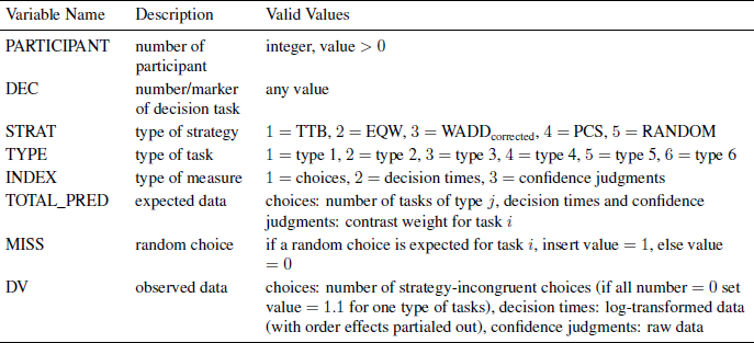
The variable “PARTICIPANT” codes the number of the participant. The variable “DEC” codes the position of the decision task in the sequence of all tasks/trials. The variable “STRAT” codes the strategy: 1 = TTB, 2 = EQW, 3 = WADDcorrected, 4 = PCS. It is not necessary to input values for RANDOM because the data vector is generated based on the data from the other strategies. The variable “TYPE” codes the type of tasks. The types differ in the configurations of the cue values (Glöckner, Reference Glöckner2009). The variable “INDEX” codes the type of measure: 1 = choice, 2 = decision time, 3 = confidence judgment. The variable “TOTAL_PRED” codes the total number of observations per type and the contrast weight for measures of decision times and confidence judgments. The variable “MISS” is used for choice data only: random choice for the specific task expected (= 1) vs. not expected (= 0). The final variable “DV” codes the observed data point of measure.
For choices, the number of strategy-incongruent choices is coded. Hence, 0 indicates that all choices for tasks of the respective task type were in line with the prediction of the strategy. In case a participant shows strategy-congruent choices for all tasks of all types, the input for “DV” should be coded as 1.1 for one type of tasks due to problems of convergence in the process of maximum likelihood estimation if the error is zero. 1.1 is used to indicate data points that were changed. The code of the MM-ML method will automatically change values of 1.1 to 1 (i.e., the maximum value of congruent choices is set to the total number of observations minus 1). Because decision times are usually highly skewed, log-transformed decision times should be coded. To account for learning effects over time it is recommended to use residuals after partialing out the order in presentation of choice tasks (which should, of course, be randomized in the experiment; log-transformations should be done before partialing out learning effects). Confidence judgments can be used without recoding.
Before you execute the code, save your data file under the directory C:\ in csv-format; the directory can be changed and modified for systems running Mac or Linux (see 3.2 for details).
For decision times and confidence judgments, a single line of the data matrix is reserved for task i, each participant, and strategy k. For choices, a single line of the data matrix is only needed for tasks of type j, each participant, and strategy k. Thus, in the example with 6 types of task and 10 tasks per type of task, there are two times sixty lines reserved for decision times and confidence judgments and only six lines reserved for choices for each participant and strategy k.
To illustrate the structure of the data file, we conclude with a short example. Assume you want to code the input for each measure (i.e., choices, decision times, and confidence judgments) for participant 6, type of tasks 1, and strategy 4 (= PCS). For the 10 tasks of type 1, participant 6 chose 10 times option A. In reference to the choices expected for type of tasks 1 and PCS (see Table 2), participant 6 made 0 strategy-incongruent choices.
In the example, there are 10 tasks of type 1. Therefore, there are two times ten lines reserved for decision times and confidence judgments for participant 6 and PCS. As a matter of simplification, we only demonstrate the input for task 1 of type of tasks 1. Participant 6 needed 3001 ms before she decided to choose one of the options. Due to the skewed distribution of decision times, the log-transformation of 3001 ms = 8.007 is the input for the data file (for simplicity we do not consider partialing out time effects here). Furthermore, participant 6 selected a confidence rating of 29 (on a confidence scale ranging from 0 to 100) that she picked the option with the higher criterion value. Therefore, 29 serves as the input for the confidence judgment of task 1 in the data file.
The coding of the three lines of the input described in the example can be found in Table 4.
Table 4: Name tags, descriptions and valid values of the variables in the data file

For all three measures, we insert a 6 for participant 6 (PARTICIPANT), a 4 for PCS (STRAT), and a 1 for type of tasks 1 (TYPE).
In the first line of Table 4, the choices are coded. We insert a 1 to set choices as the type of measure (INDEX). We expect 10 choices congruent to PCS (TOTAL_PRED). Participant 6 made no strategy-incongruent choices. Thus, we insert 1.1 for the observed value (DV). We did not expect random choices for PCS and type of tasks 1; therefore we insert a 0 for the random choice indicator (MISS).
In the second line of Table 4, the decision time is coded. We insert a 2 to set decision times as the type of measure (INDEX). The contrast weight for type of task 1 is −0.444 (TOTAL_PRED). We have observed a log-transformed decision time of 8.007 (DV). For decision times, the coding for random choices is not relevant. We therefore insert a 0 for random choices (MISS).
In the third line of Table 4, the confidence judgment is coded. We insert a 3 to set confidence judgments as the type of measure (INDEX). The contrast weight for type of task 1 is 0.621 (TOTAL_PRED). We have observed a confidence judgment of 29 (DV). For confidence judgments, the coding for random choices is not relevant. We therefore insert a 0 for random choices (MISS).
We can further insert a marker for each line in the data file (DEC). Entries in the DEC vector are not processed during the maximum-likelihood estimation in R. Nevertheless, it makes sense to code the order of appearance of the task in the experiment to investigate order effects for decision times and confidence judgments before applying the MM-ML method. Due to the coding of choices, you can insert a marker only for each type of task for choices.
3.2 Input and output
To modify the MM-ML code, just open and change values in the MM-ML.R file with your preferred text-editor. The user input is at the beginning of the file, perceptually segregated from the program code. To run the code, just copy the code of the MM-ML.R file in the open R Console, or submit it with source(‘MM-ML.R’) from the R command line.
In the “user input”, you can set the directory where the data file is located.
The program produces two outcome variables: “output” and “likbic” (see 3.2). Both variables are printed in the R Console and saved in csv files by default under the directory C:\. (We use Windows conventions in this exposition. In all cases, users of Linux, Unix, or OS-X can replace the working directory without the C:\ prefix.) The variable “output” stores estimations of coefficients, corresponding standard errors, z-values, probabilities for absolute z-values, and confidence intervals for each participant and strategy. The variable “likbic” stores the BIC and log-likelihoods for each participant and strategy. The output display is similar to the STATA output described in Glöckner (Reference Glöckner2009, p. 195).
Furthermore, you can easily inactivate/activate code sections, e.g., whether to read in raw data, run maximum likelihood estimations, print output, and save output; see “inactivate/activate code sections” in the code for details. This enables you to print the output for further participants without having to re-run the entire code.
By default, R will print the output for all participants and strategies. For purposes of clarity, you can also print the output for a specified participant and strategy; see “output: print selection of coefficients …”.
Finally, you can specify the maximum number of iterations and the relative criterion of convergenceFootnote 2 for the BFGS maximum likelihood estimation algorithmFootnote 3 (Broyden, Reference Broyden1970, Fletcher, Reference Fletcher1970, Goldfarb, Reference Goldfarb1970, Shanno, Reference Shanno1970) in “configure the properties of maximum likelihood algorithm (mle)”. Defaults should be fine for most applications. For the unlikely case that the maximum likelihood estimation algorithm does not converge for a strategy of a participant, you can easily increase the maximum number of iterations (see comments in the code).
3.3 Example
In the supplementary material, you will find the file data.csv. Please copy this file into the directory C:\. In the data file, there are codings for 10 participants, 6 task types, and 10 tasks for each type of task; see Glöckner (Reference Glöckner2009; Reference Glöckner2010) for details. First, we suggest you run the MM-ML method for all participants and strategies. You need to open the file MM-ML.R with a text editor, set the variable “totalprint” in the section “inactivate/activate code sections” to a value of 1 (= default value), and copy/paste the entire code into the open R Console, or submit it from the command line.
If you require individual predictions for a specific person and strategy, you can modify the variables “participantOUT” and “strategyOUT” in the section “output: print selection of coefficients …” as in the following example. Assume one wants to print the log-likelihoods and BIC values for all strategies for participant 6. Simply set “participantOUT” to a value of 6. Next, select all text, copy it, and paste it into the open R Console (or submit from the command line).
Based on the BIC values of the output (see Table 5, top), participant 6 most likely followed the PCS strategy (in comparison to all other tested strategies).
Table 5: Example output of the R implementation of the Multiple-Measure Maximum Likelihood Strategy Classification Method
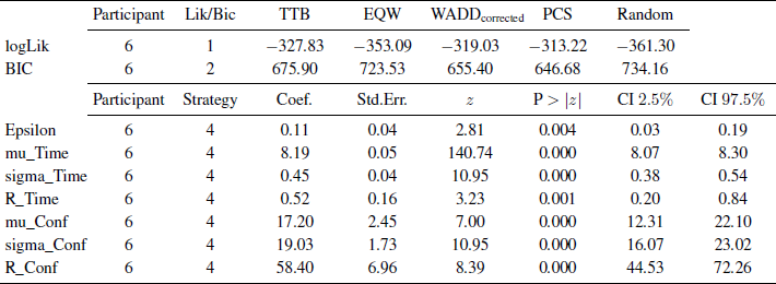
Note. The output of the log-likelihoods and BIC values for participant 6 and all strategies (top) and the coefficients for participant 6 and strategy 4 (= PCS) (bottom) are shown.
To print out the coefficients for participant 6 and PCS, set “strategyOUT” to a value of 4. To prevent R from re-reading the entire raw data and repeating the maximum likelihood estimation, disable these code sections by setting “readdata” and “mml” in “inactivate/activate code sections” to a value of 0. Again, select all text, copy it, and paste it into the open R Console (or submit). This produces the output (see Table 5, bottom) for all coefficients, e.g., єk, µT, σT, RT, µC, σC, and RC along with the corresponding test statistics. In the example, all coefficients are significantly (p<.05) different from 0.
3.4 Generalization
The provided R code cannot be applied to just the default strategies. It is flexible enough to enable you to estimate the parameters and obtain the fit for most strategies you would like to test. The only constraint is that your strategy needs to match the number of parameters estimated for one of the strategies described in the article. This is the case if (a) the strategy to be considered makes clear predictions concerning choices (i.e., option A, option B, or guessing) and (b) if the data set contains task types for which the strategy predicts differences in decision times and confidences. For such a strategy, all parameters described in Table 1 are estimated. To analyse such a strategy, you generate the expected choices and contrast weights for decision time and confidence in accordance with the predictions of your strategy and set STRAT = 1 or 4 (currently used for TTB or PCS) in the raw data file. Alternatively, if the additional strategy predicts equal decision times for all task types, it includes all parameters except for RT. In this case, you proceed as described above, but you set STRAT = 2 or 3 (currently used for EQW or WADDcorrected). Finally, you should adjust strategy labels that are displayed in the output in “set strategy labels” accordingly. Note that the MM-ML estimations for strategies are independent of each other. It is therefore theoretically possible to compare as many strategies as one needs by re-running MM-ML with additional strategies. Finally, the code does not only allow testing the specific number of tasks and type of tasks used in the example. It is possible to change the number of task types and the number of tasks for each task type without having to change code. The number of free parameters for the BIC value is adjusted automatically. Therefore, MM-ML users are by no means limited to relying on six task types and ten tasks of each type. We use them only as one example.
3.5 Implementation of MM-ML as R-function
The generalized version of the MM-ML method is implemented as an easy-to-use R function. To improve usability, the function uses a more convenient format of the raw data file.
The raw data file consists of 6 columns. The first three indicate the number of the participant (“PARTICIPANT”), the number of the decision task (“DEC”), and the type of the task (“TYPE”). The fourth column “ACHOICES” codes whether the participant chose option A (coded as 1) or option B (coded as 0) in this task. In the fifth column, the decision time of the participant for the task is indicated (“DECTIMES”). In the sixth column, the confidence judgment for the task is coded (“CONFJUDGMENTS”). Hence, all data concerning one choice task is now coded in one line. Furthermore, choices do not need to be aggregated by the user, and expected choices and contrasts do not need to be specified for every single strategy. If you did not assess decision times and/or confidence judgments, just delete the respective columns in the data file. In the supplementary material you find a data file in the respective simplified format (datafunction.csv; which is a reformatted version of the original data file data.csv).
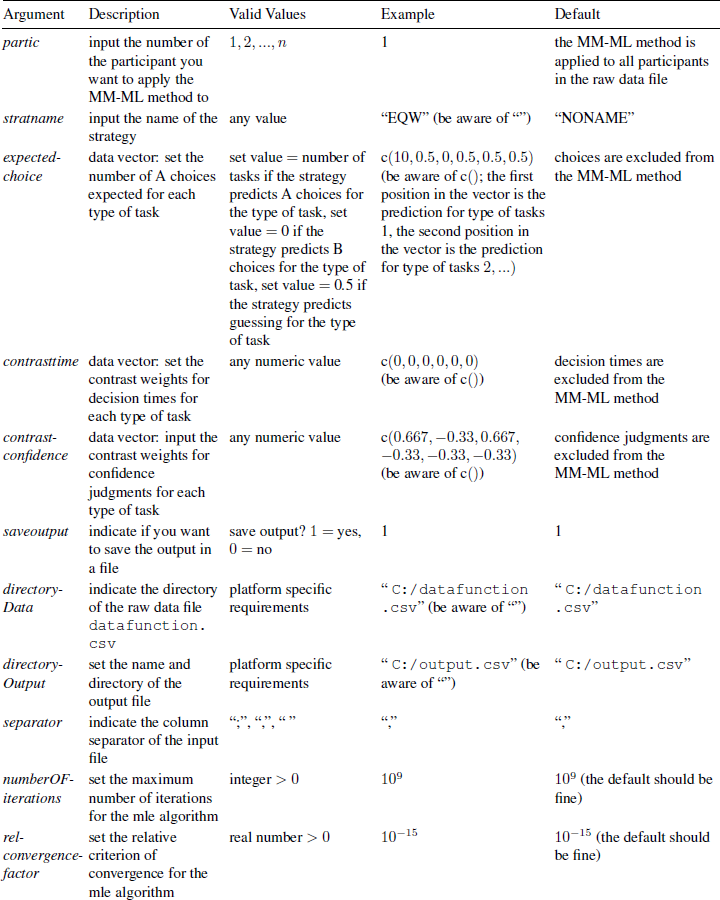
To use the MM-ML method function, you need to copy and paste (or submit) the code provided in the file FunctionMM-ML.R. To call the function afterward, type the command: in the open R console and hit enter. If an argument of the function is left blank, the default is applied. Arguments, descriptions, valid values, examples and defaults are listed in the Appendix.
MMML(partic, stratname, expectedchoice, contrasttime, contrastconfidence, saveoutput, directoryData, directoryOutput, separator, numberOFiterations, relconvergencefactor)
For example, to estimate the parameters and assess the fit for the TTB strategy described in section 2.2 for all participants in your dataset and keep the defaults for all other arguments of the function, type: in the open R Console and hit enter. Because partic was not specified, estimates for all participants are generated. Estimates of the parameters, log-likelihoods and BICs are prompted in the R Console and are saved in the file output.csv under directory C:\. In case you did not assess decision times in your study and do not want to save the output, you can leave the fourth argument of the function blank and input a 0 for saveoutput, i.e, you type:
MMML(,“TTB”,c(10,10,10,10,10,10), c(−0.167,−0.167,−0.167,−0.167,−0.167,0.833), c(0.167,0.167,0.167,0.167,0.167,−0.833))
MMML(,“TTB”,c(10,10,10,10,10,10), , c(0.167,0.167,0.167,0.167,0.167,−0.833),0).
It should be clear now that you can test further strategies by simply changing the expected choices and contrast weights in the MM-ML function. You can exclude measures from the MM-ML method by leaving the argument expectedchoice and/or contrasttime and/or contrastconfidence in the function blank. Again, the number of task types and the number of tasks per type can be altered without the need to change code.
Finally, we included the following features that will further simplify usability. First, it is unnecessary to input contrast weights that meet the scaling properties discussed in section 2.2, i.e., sum of contrast weights = 0 and range of contrast weights = 1. The user can input the “raw” contrast weights, i.e., c(4,4,4,4,4,10) for TTB contrast weights. The function rescales the contrast weights automatically. Second, the function automatically adds or subtracts one strategy congruent or incongruent choice if a participant shows strategy congruent or incongruent choices (or mixed) for all task types (see section 3.1). Automatic addition or subtraction of a choice is prompted in the output in the R Console.
4 Final comment
The code of the MM-ML method in R should enable researchers easily to identify participants’ decision strategy in complex decision tasks. Beyond the benefit of strategy classification, the MM-ML method facilitates thinking about strategies on a detailed process level. To apply the MM-ML method, researchers have to specify the process and outcome characteristics of a strategy. The MM-ML method can therefore be used as a tool for constructing new strategies and improving existing strategies of decision making. All it necessitates is clearly specified models. Besides estimating the overall fit of observed data to the predictions of the different strategies, the method allows the investigation of process properties in more depth. In particular, you can ask whether the scaling parameters for time RT and RC confidence contribute significantly to predicting the data per individual. If this is not the case, predictions for the respective dependent measure and possibly also assumptions about underlying processes should be rethought.
Appendix: MMML() function in R
Arguments, descriptions, valid values, examples, and defaults.
