


Introduction
Apiculture is an important agriculture friendly and economically viable activity that incorporates agroforestry, agricultural activities, and forest management (Burgett, Reference Burgett, Fisher, Mayer and Johansen1984). In apiculture, honeybees are vital pollinators that are crucial for plant diversity, agricultural sustainability, providing food security, and environmental protection (Graham,Reference Graham1992; Akhila et al., Reference Akhila, Manjunataha and Keshamma2022). Approximately one-third of the world's human nutritional supply comes from crops pollinated by bees. Despite increasing worldwide demand for agricultural pollination services, honeybee populations are struggling to maintain their own viability due to widespread habitat loss and fragmentation (Cornman et al., Reference Cornman, Tarpy, Chen, Jeffreys, Lopez, Pettis, van Engelsdorp and Evans2012). Rapid colony death accompanied by a scarcity of healthy worker bees within the hive is a major symptom of colony collapse disorder. It is a complex problem that is impacted by numerous local and regional factors. Urbanisation, deforestation, and agricultural intensification are limiting the availability of suitable habitats for honeybees (Shaher, Reference Shaher and Manjy2020). Additionally, parasitic infections and mites causing serious consequences, including reduced honey production, weakened colony, and even colony loss (Cornman et al., Reference Cornman, Tarpy, Chen, Jeffreys, Lopez, Pettis, van Engelsdorp and Evans2012). Honeybees are also encountering an increasingly diverse range of detrimental impacts due to extensive application of chemicals and pesticides, pollution, climate change, genetically modified organism agriculture, insufficient food sources, and loss of forage, affecting development of crops and their nutritional value (Neumann and Carreck, Reference Neumann and Carreck2010).
Several research initiatives have been accomplished to enhance the general health of honeybees and enhance apiculture practices (Alves et al., Reference Alves, Pinto, Ventura, Neves, Biron and Junior2018; Paolillo et al., Reference Paolillo, Petrini, Casiraghi, De Iorio, Biffani, Pagnacco, Minozzi and Valentini2022). These initiatives encompass the exploration of honey bee pathologies and parasites, along with the determination of optimal management strategies to monitor honey bee health, brood development, and habits (Liew et al., Reference Liew, Lee and Chan2010; Hoferlin et al., Reference Hoferlin, Hoferlin, Kleinhenz and Bargen2013; Rathore et al., Reference Rathore, Tyagi and Agrawal2023). Beehive management practice is helpful to examine topics like colony development food storage dynamics (Alves et al., Reference Alves, Pinto, Ventura, Neves, Biron and Junior2018), brood production, and adult worker lifespan, as well as the impact of apiary location and farming methods on honey bee health. Colony growth is also measured to determine the efficacy of Varroa destructor management strategies (such as drone removal, colony splitting, formic acid treatments, and oxalic acid treatments) (Neumann and Carreck, Reference Neumann and Carreck2010).
Maintaining healthy colonies of honey bees is essential for productive beekeeping. This metric represents health and fitness of bees which affects the yield of honey and the availability of foragers to provide pollination services. Timely diagnosis of bee brood development and hive health, not only prevent colony loss but also helps in increasing the agricultural productivity. Traditional beehive monitoring technique (Liebefeld method) is time consuming as it is based on a visual estimation resulting in variability and erroneous observation. Another drawback is that the colony estimating task necessitates competent and qualified beekeepers. Thus, beekeepers and researchers require an automated and reliable tool that can access colony strength remotely and keep the records of visual estimations and data for the further analysis. The available data will aid enhancing honey production and early treatment of pathologies.
Several automatic and semi-automatic comb image evaluation tools were developed over time. Researchers have accomplished objectives like detecting capped and uncapped brood area (Emsen, Reference Emsen2006), counting total number of cells in comb pictures (Liew et al., Reference Liew, Lee and Chan2010; Rathore et al., Reference Rathore, Tyagi and Agrawal2023, Sparavigna, Reference Sparavigna2016a, Reference Sparavigna2016b), colony size (Cornelissen et al., Reference Cornelissen, Schmidt, Henning and Der2009), brood growth (Hoferlin et al., Reference Hoferlin, Hoferlin, Kleinhenz and Bargen2013), capped brood and capped honey cell (Colin et al., Reference Colin, Bruce, Meikle and Barron2018), cell classification (Jeker et al., Reference Jeker, Schmid, Meschberger, Candolfi, Pudenz and Magyar2012; Alves et al., Reference Alves, Pinto, Ventura, Neves, Biron and Junior2018; Paolillo et al., Reference Paolillo, Petrini, Casiraghi, De Iorio, Biffani, Pagnacco, Minozzi and Valentini2022) using various methods. Emson (Reference Emsen2006) used Photoshop CS2's colour tool to semi-automate brood area measurement. Liew et al. (Reference Liew, Lee and Chan2010) detect and count the cells using Hough transform technique and achieved an accuracy of 80%. Yoshiyama et al. (Reference Yoshiyama, Kimura, Saitoh and Iwata2011) segment capped brood area using Adobe Photoshop and classified the cells manually. Larvae Area plugin was created using an image processing software, ImageJ (https://imagej.nih.gov/ij/index.html). This plugin calculates capped and uncapped cell areas automatically. Rodrigues et al. (Reference Rodrigues, Neves and Pinto2016) proposed an automatic cell counting method based on circular convolution. This method utilises a circular mask to identify region of interest (ROI) and then calculates the difference in intensities between the pixels on cell walls and pixel intensity inside the cell. The interior of cell is darker compared to cell wall, hence it is a useful feature. It was determined that the detection rate of cells was 99.04% accurate.
Wang and Brewer (Reference Wang and Brewer2013) proposed pattern recognition algorithms for the detection of honey bee cells. HiveAnalyzer (Hoferlin et al., Reference Hoferlin, Hoferlin, Kleinhenz and Bargen2013) classifies comb cells using linear Support Vector Machine with multi-scale Haralick features and colour histograms. The cell contents are classified in seven classes with 94% accuracy for high-confidence cells. A semi-automated tool Combcount (Colin et al., Reference Colin, Bruce, Meikle and Barron2018) detects capped and uncapped honey cells. However, a user has to segment both the area manually using a selection tool. A software called DeepBee (Alves et al., Reference Alves, Pinto, Ventura, Neves, Biron and Junior2018) is capable of automatically detecting cells in comb images and classify their content in seven different classes. The dataset was tested on various different convolutional neural network (CNN) architectures to get the best results. Further, Chaudhary et al. (Reference Chaudhary and Pachori2021a, Reference Chaudhary and Pachori2021b, Reference Chaudhary and Pachori2022, Reference Chaudhary and Pachori2023) suggested feature extraction methods such as Fourier–Bessel series based expansion method for feature extraction and LS-SVM for classification of medical images. Paolillo et al. (Reference Paolillo, Petrini, Casiraghi, De Iorio, Biffani, Pagnacco, Minozzi and Valentini2022) proposed a semi-automatic method that employs automatic colour equalisation technique along with three different thresholding techniques for cell segmentation to locate cells under uncontrolled illumination and noise artefacts.
Unfortunately, all the strategies proposed so far have achieved cell detection which gives no information about the cell content. The effect of noise and its measurement in terms of peak signal to noise ratio (PSNR) and structural similarity index measurement (SSIM) (Fareed and Khader, Reference Fareed and Khader2018) have not yet been considered. All methods have only been tested on closely supervised research images limiting generalisability of the findings. Further, the existing techniques are semi-automatic involving human intervention making it time inefficient and laborious.
This research focuses on the utilisation of deep learning techniques in the field of apiculture to identify the cells in honey comb images and classify them to estimate the brood stage efficiently and accurately in less time. By leveraging these advanced technologies, we aim to streamline and optimise hive management task which involves developing and deploying intelligent algorithms that can learn from data and make informed decisions autonomously.
Material and method
In this study, we examined deep learning techniques for analysing datasets, denoising and enhancing them for three distinct CNN models in order to accomplish the required outcomes. The present study has devised an automated mechanism for identifying and localising cells through a deep learning framework. Herein, inception version three model has been updated with different optimisers and objectives that enhances the detection speed while simultaneously decreasing the parameter count.
Image dataset
To carry out the research, we have created two datasets one for segmentation and another for classification. The Image dataset in the segmentation process includes 62 (3856 × 5787 px size) beehive frame images (Apis cerena indica) and their corresponding masks. The masks were created using Adobe Photoshop masking tool. Prior to the segmentation, images were preprocessed using a denoising filter followed by contrast enhancement to emphasise the comb cell boundaries and features. Further, these 62 images were fragmented in small patches of 482 × 482 each to create dataset of 6448 images. These 6448 images were further downscaled to size 224 × 224 to train the segmentation model. The segmentation has been implemented for binary classification that detects ROI from the background. The training data contains 6448 images of size 224 × 224 out of which 80% of data (I_train) is used for training and remaining 20% of data was used for testing (I_test) and validation (I_val). After segmentation, individual cells were detected using circle Hough transform (CHT) technique.
Further, detected cells were given to the classification model. Since bee brood analysis has been done for three classes (egg, larvae, and pupa), the detected cells were labelled in three classes. A total of 15,000 labelled cell images were utilised in the creation of the classification dataset. These images underwent additional augmentation using a data augmentation technique (scaling, rotation by 90° and inversion), resulting in the dataset comprising 45,000 images. Further, the cell classification network was trained with these 45,000 cell images each having size of 224 × 224. Dataset was split into training set (X_train, Y_train), testing set (X_test, Y_test) and validation set (X_val, Y_val). 80% of the data were used for training, 10% for testing, and 10% for validation. Pre-processing algorithms were implemented in Google Colab (https://colab.google/) using Python OpenCV2 v.4.0 package (version 3.10) and the CNN architectures were built with tensor flow 2.11.0 and keras 2.11.0 on processor Intel Core i5 8250U CPU 3.5 GHz with 16 GB of RAM.
Image pre-processing
The objective of pre-processing is to enhance the picture data by minimising unintended distortions or boosting certain visual characteristics necessary for subsequent processing. The image capturing instruments and poor lightning circumstances may degrade the quality of image (Gómez et al., Reference Gómez, Valenzuela and Valenzuela2022). Images acquired in poor light are susceptible to reduced visibility, which can impede the functionality of various computational photography and computer vision systems. Pre-processing is a technique that improves features such as cell edges, contrast, colour, and other important aspects necessary for the intended application. In addition to this, it also downscales and augments images to improve the model's learning capacity. The image pre-processing pipeline contains illumination normalisation and colour enhancement, edge enhancement, and image filtering.
Illumination normalisation and colour enhancement
The images were recorded at various times throughout the day and camera flash light introduced an additional brightness to the image that appears as a white spot in the cells which can be wrongly detected as an egg. The complexity of cell categorisation increases due to nonlinearity in the variance of illumination. Hence, to counteract the impact of lightning changes, illumination normalisation and colour enhancement is required. In this research, automatic colour enhancement (Plutino et al., Reference Plutino, Barricelli, Casiraghi and Rizzi2021, Rizzi et al., Reference Rizzi, Gatta and Marini2003). Followed by histogram equalisation technique (Gómez et al., Reference Gómez, Valenzuela and Valenzuela2022) was employed for the purpose of colour enhancement and light normalisation.
Edge enhancement
The enhancement and identification of edges are both essential components of object detection algorithms since edges constitute an object's morphology. In honeycomb frame images, the outer edges of cells are brighter compared to the inner sides, creating the appearance of a dark hole. These boundaries of the cells need to be emphasised for correct detection. In this research we have employed contrast limited histogram equalisation (CLAHE) technique to perform edge detection. CLAHE is effective in enhancing local contrast in image with varying illumination condition (Shelda and Ravishankar, Reference Shelda and Ravishankar2012; Gómez et al., Reference Gómez, Valenzuela and Valenzuela2022).
Image filtering
In the pre-processing pipeline, a wavelet denoising filter has been introduced. Wavelet filter provide an advantage of selectively emphasising and de-emphasising image details in certain spatial frequency domains (Ellinas et al., Reference Ellinas, Mandadelis and Tzortzis2004; Saxena and Rathore, Reference Saxena and Rathore2013). Image and signal denoising with wavelet thresholding frequently employs wavelet transformation as one of the key techniques. It is a non-linear technique that decomposes image into different frequency components (Donoho, Reference Donoho1995). Each wavelet is then processed, convolved and shifted across image to capture information at different time or spatial locations, extracting local details at different scales.
Consider an original image f(m, n) affected by Gaussian noise g(m, n), then the noisy image η(m, n) is given by
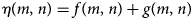
Apply the wavelet transform to equation 1 to obtain wavelet coefficient C n(m, n) for noisy image given by equation 2

where, C f(m, n) wavelet coefficients of original image and C g(m, n) wavelet coefficients of noise. We have used a universal threshold value to adjust the C n(m, n) in order to remove noise from the image, f(m, n)
where ‘th’ is the threshold value, C(m, n) is the wavelet coefficient with high frequency of wavelet decomposition and $\hat{f}( {m, \;n} ) \;$ is the estimated wavelet coefficient from thresholding process. The threshold value is proportional to the standard deviation of noise and defined as:
where σ 2 is the variance of noise and M is total number of image pixels. Attenuating high frequencies results in a smoother image in the spatial domain. Conversely, attenuating low frequencies results in the enhancement of edges (Ellinas et al., Reference Ellinas, Mandadelis and Tzortzis2004; Jyoti and Abha, Reference Jyoti and Abha2013; Saxena and Rathore, Reference Saxena and Rathore2013).
Image segmentation
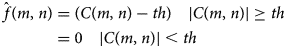
The initial stage in cell detection is localisation, or identifying the precise area (ROI) where cells are located. Cropping the image manually (Liew et al., Reference Liew, Lee and Chan2010; Paolilo et al., Reference Paolillo, Petrini, Casiraghi, De Iorio, Biffani, Pagnacco, Minozzi and Valentini2022), or automatically, through the use of computer vision methods are two viable ways for achieving this. Traditional (manual) cropping practices have largely been abandoned due to their inefficiency. This paper utilises CNN-based automatic segmentation technique proposed by Ronneberger et al. (Reference Ronneberger, Fischer and Brox2015) to determine ROI, which makes our work more manageable and precise. The model performs the pixel level classification that classifies images by clustering pixels of the same object class. This type of segmentation is referred as semantic segmentation (Thakker, Reference Thakker2019; Thoma, Reference Thoma2016). The proposed CNN architecture for segmentation mainly has two parts, encoder (contraction) and decoder (expansion). The encoder network operates as the feature extractor and acquires a conceptual representation of the input image through a sequence of encoder blocks. The Encoder block is composed of four convolutional blocks, each containing two consecutive 3 × 3 convolutional layers with ReLU activation function, separated by a dropout layer with a range of 0.2–0.3. Subsequently, a 2 × 2 maximum pooling operation is executed with a stride of 2 to perform downsampling. The initial layer has 16 filters of kernel size 3 × 3 which is doubled with each subsequent convolutional layer and the last layer has 256 filters. In between contraction and expansion layer, a bottleneck layer with two convolutional block followed by dropout and max pool layer is used. The feature map from bottleneck layer is upsampled to the size of input image. The skip connection is used to create the segmentation map learned from the features obtained from the encoder block.
Fig. 1 depicts the architecture of segmentation model proposed in this study. There are four 2 × 2 convolution blocks in the decoder pipeline. Each convolution cuts the number of feature channels in half and concatenates them with corresponding images from the down sampling path. The convolution layer is followed by 3 × 3 filters with ReLU activation function. The training of the model involved 6448 images, each with a size of 224 × 224. During the training phase (I_train), 80% of the data is utilised, while the remaining 20% is utilised during the testing and validation phases (I_test, I_val). The model was trained for 40 epochs with a Learning Rate (LR) of 0.001 and compiled using the Adam optimiser and binary cross entropy loss function.
Figure 1. Architecture of segmentation model.
Cell localisation
The internal structure of a beehive possesses hexagonal cells composed of bee wax that are arranged in a regular pattern and appear as circles from a distance. Therefore, in this research we have used Hough transformation (HT) technique for cell detection. The Circular Hough Transformation (CHT) (Rhody, Reference Rhody2005; Rizon et al., Reference Rizon, Yazid, Saad, Shakaff, Saad, Sugisaka, Yaacob, Mamat and Karthigayan2005), has numerous uses in the field of object detection, including biometric systems (Wu, Reference Wu2019), the identification of regions in images, and many more. The HT and various modified variants have been acknowledged as reliable curve identification tools that depend on a voting procedure which determines the likelihood that a given pixel with coordinates (a, b) lies on a circle. This is done by using the equation for a circle to generate a three-dimensional parameter space, which is used to aggregate votes in order to search for circles with a specified radius, R. The accumulator accumulates these votes for all parameter combinations for each feature point. The cells with greater number of votes are marked as centres. CHT detects cells that have cell radius in range of minRadius, maxRadius and the distance between cells. In order to obtain optimised parameter, a grid search is performed for minRadius equal to 10 and maxRadius equals to 45. The minimum distance between two detected cell is kept 12 to avoid false detection and the canny threshold is set to 150. The CHT iterates the following equations to identify the centre coordinates (x, y) of every locus (a, b) of circles in the image
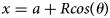
where R is the radius and theta (θ) is the line orientation. Every edge pixel in the x − y space will be equivalent to a circle in the parametric space.
Cell classification
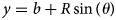
Throughout the course of a bee colony's lifecycle, the comb cells are occupied by a variety of immature phases as well as various sources of food. Honeybees normally lay only one egg per cell, which develops into a larva and pupa, therefore classification of newly discovered cells is necessary to get insight on the behaviour and growth of the brood. Here in this research, we proposed an enhanced Inception-v3 model for automatic classification of cells. Szegedy et al. (Reference Szegedy, Ioffe, Vanhoucke and Alemi2016a, Reference Szegedy, Vanhoucke, Ioffe and Shlens2016b) suggested the Inception model to mitigate the impact of computing efficiency and low parameters in practical applications. Inception-v3 uses CNN architecture inspired by GoogleNet to resolve deep learning challenges of Inception-v2. Further, transfer learning is merged with the Inception-v3 (Zuhang et al., Reference Zuhang, Qi, Duan, Xi, Zhu and He2019; Gómes et al., Reference Gomes, Barddal, Enembreck and Bifet2017) model to improve the learning efficiency of the model and to better extract the deep-level features of cells. This approach improves the robustness and generalisability of the model and converges the model faster. Transfer learning is a process which is used to transfer feature extraction layer weights from a learned model over a dataset to another model that will be trained in a new dataset. Herein, we have used weights pre-trained on ImageNet dataset (Krizhevsky and Hinton, Reference Krizhevsky and Hinton2009, Krizhevsky et al., Reference Krizhevsky, Sutskever and Hinton2012) to extract low level features. To test the robustness of the model, we performed cell classification with the standard Inception-ResNet-v2 (Szegedy et al., Reference Szegedy, Ioffe, Vanhoucke and Alemi2016a, Reference Szegedy, Vanhoucke, Ioffe and Shlens2016b; Nguyen et al., Reference Nguyen, Lin, Lin and Cao2018; Demir and Yilmaz, Reference Demir and Yilmaz2020) and Inception-v3 model. The Inception-ResNet-v2 model's structure is depicted in fig. 2 is a deeper version of Inception-v3 which uses the residual connection and inception structure. Residual connections integrate multiple-sized convolutional filters in the Inception-ResNet-v2 block that minimises training time and avoid deep structural deterioration. The base model is trained using transfer learning approach with the image of size 299 × 299. Here, a dense layer with the ReLU activation function has been added with the drop rate of 0.25.
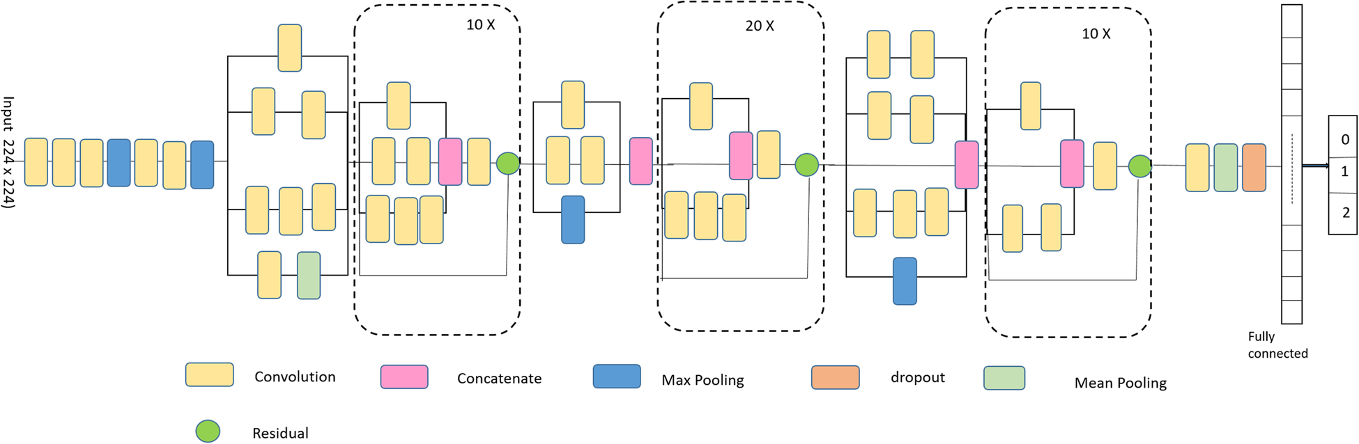
Figure 2. Architecture of Inception-ResNet-v2.
As shown in fig. 3, the proposed model is based on Inception-v3 model. For fine tuning and creating specific learning, we modify the model by adding four layers at the end of the architecture. The first layer was a dropout layer applied before the fully connected layer. Dropout layer introduces a regularisation mechanism which improves the model's generalisation and prevents overfitting. Afterwards, we included three dense layers with the first one having 1024 neurons followed by a hidden layer with 256 neurons and the last one having three neurons and a Softmax activation function to represent our classes in a linear probabilistic domain. Here, in this model the size of input image was kept as 224 × 224, this subsequently sped up the classification process, while producing less effect on the feature classification.
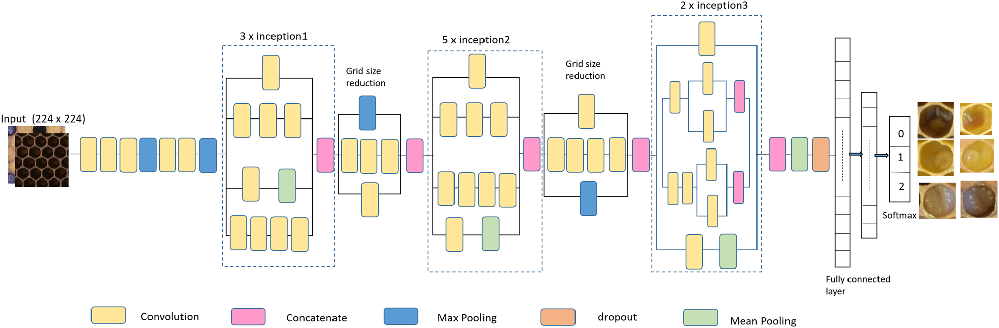
Figure 3. Architecture of enhanced Inception-v3 for cell classification.
The model was trained with 45,000 images of size 224 × 224 and complied with Adam optimiser and Categorical cross entropy loss function with learning rate of 0.001. The hyperparameters have been adopted as follows: batch size = 16, momentum = 0.6, weight decay = 0.0001 and metric of evaluation is Validation accuracy. To evaluate the performance of the proposed model, a series of experiments were conducted with three distinct models and their results have been compared to determine their relative performance.
Results
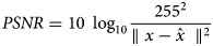
This section explores the metric data and experimental findings obtained by the proposed models to determine the optimal parameter settings for accurate cell detection and classification. Preprocessing of images is necessary to enhance the perception and interpretability of information contained in the image before performing cell detection. The preprocessing pipeline utilises the frequency domain filter technique to achieve comprehensive optimisation of images, in addition to edge enhancement and shadow suppression. To assess the performance metrics of image denoising techniques, PSNR and SSIM have been used as illustrative quantitative measurements. For a given original image x, the PSNR of a denoised image $\hat{x}$ is given by:
The SSIM index is also determined by
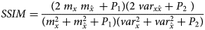
where, m x, $m_{\hat{x}\;}$ , ${\mathop{\rm var}} _x$
 and ${\rm va}{\rm r}_{\hat{{\rm x}}}$
 are mean and variance of x and $\hat{x}$
 , $\sigma _{x\hat{x}}$
 is the covariance between x and $\hat{x}$
 and P 1, P 2 are the constants used to avoid instability. During the experiment, it has been observed that the spatial filters caused blurring of sharp edges and significant features, while simultaneously eliminating high frequency noise. Conversely, the proposed wavelet filters were able to remove noise while preserving the integrity of the edges. The average PSNR and SSIM evaluated for 100 unprocessed images is 22.13 dB and 0.525, whereas average PSNR and SSIM for preprocessed images is 29.64 dB and 0.752.
After pre-processing, images are segmented to obtain area of interest and to localise cells automatically. Automatic beehive cell detection using CNN is tested over 100 preprocessed images. The metrics for cell detection is given by equations 9–11
where, AC (automatic count) is the total number of cells detected, MC (manually count) is the total number of cells counted manually, TPC (true positive counts) is the total number of cells detected correctly, FPC (false positive counts) is the total number of cells detected on inexistent cells and FNC (false negative count) is the total number of cells that remained undetected. Cell detection was performed on both preprocessed and unprocessed images and detection accuracy (CDA) has been calculated with respect to the manual count. The average cell detection accuracy (CDA) achieved is 94.32% with the noisy images. It has been observed that a significant number of cells remain unpredictable, resulting in an increase in the number of false negative classifications (FNC). It is due to the reason that the walls of honeybee cells are very thin and their edges may easily get distorted in the presence of noise, leading to unpredicted and wrongly predicted cells. However, after preprocessing and denoising, the cell detection accuracy has achieved up to 97.03%. Experimental outcomes show that the proposed methodology improves the contrast and sharpness of the image resulting in better visibility of edges hence yielding a higher number of true positive counts and a lower number of unpredicted cells.
After performing cell detection, the cells are classified for three classes (egg, larvae, and pupa) and further, cell classification was performed on three different models (Inception-ResNet-v2, Inception-v3 and Enhanced Inception-v3). Table 1 tabulates the test accuracy for all models. Inception-ResNet-v2 and Inception-v3 model are trained for 40 epochs, and Enhanced Inception-v3 for 35 epochs. During the training process, it is observed that suggested Enhanced Inception-v3 model exhibited no further changes in loss after 35 epochs and converged faster compared to the other two models. The hyperparameters for the model have been set as batch size = 16, momentum = 0.6, and weight decay = 0.0001. The training dataset is augmented before training the model to improve the training accuracy. The training accuracy acquired for Inception-ResNet-v2, Inception-v3 and enhanced Inception-v3 are 98.52, 98.94 and 99.31% respectively as shown in fig. 4. Although the training accuracy for all the models are projected to be met, the validation accuracy score is observed to have deviated. The validation accuracy for Inception-ResNet-v2 and Inception-v3 is achieved upto 94.78 and 96.73% respectively. Based on empirical evidence, it has been observed that Inception-ResNet-v2 experiences overfitting during training due to its greater inception depth. This is demonstrated by the increasing cross-entropy loss of 21.41% in subsequent epochs. As a result of this, the cell classification accuracy (CCA) with the Inception-Resnet-v2 found to be least among all. However, Inception-v3 extracts lesser features compared to Inception-ResNet-v2, it does not over fit the model and hence achieved the validation accuracy upto 96.73% with the decrease in validation loss of 12.56%.
Table 1. Accuracy and loss score for different CNN models
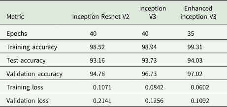
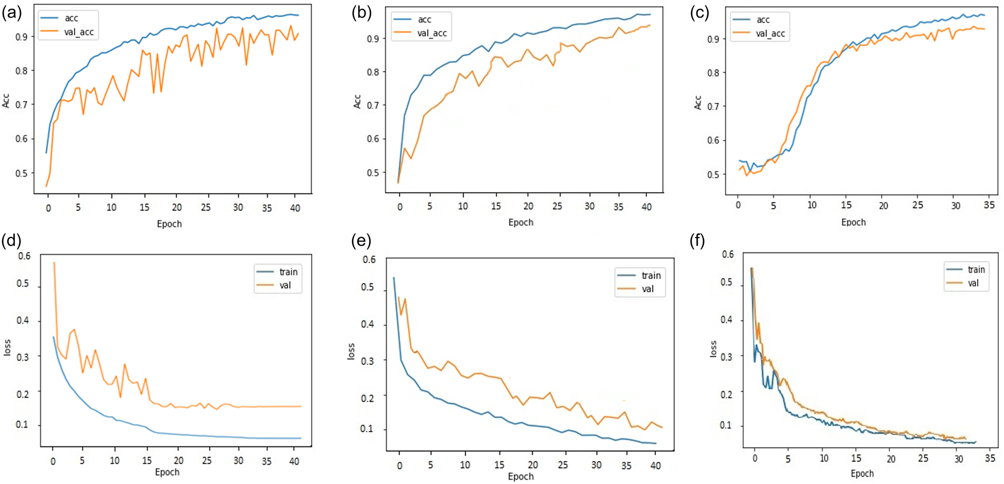
Figure 4. (a) Accuracy plot for Inception-ResNet-v2 (b) Accuracy plot for Inception-v3 (c) Accuracy plot for enhanced Inception-v3 (d) Loss plot for Inception-ResNet-v2 (e) Loss plot for Inception-v3 (f) Loss plot for enhanced Inception-v3.
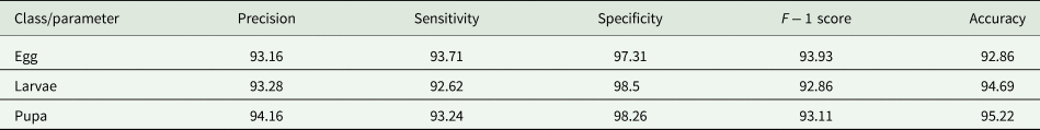
The Enhanced Inception-v3 model maximised training accuracy with 99.31% and validation accuracy with 97.02%. The proposed model exhibits better predictive capabilities when compared to Inception-ResNet-v2 and Inception-v3, as it has yielded more favourable cross-entropy outcomes. The model includes two fully connected layers consisting of 1024 units and 256 units, that selects the best features and achieved the highest accuracy. Additionally, batch normalisation (BN) has been incorporated into Inception-v3 to alleviate the distribution discrepancy between inputs and outputs in a conventional deep neural network. The learning effect is enhanced by normalising the input to each layer. During the analysis of training and testing accuracy, it was observed that the Inception-v3 model with suggested enhancements achieved a cell classification accuracy (CCA) of 94.03%, which is higher than the other models. The accuracy of cell classification was evaluated using precision, sensitivity, specificity, accuracy, and F1 score. The equations for metrics are provided as follows:
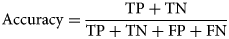
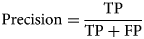
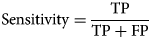
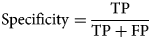
where, TP (true positive) and TN (true negative) refer to cells that have been accurately identified. On the other hand, FP (false positive) and FN (false negative) denote cells that have been inaccurately classified. Table 2 tabulates the results of Inception-Resnet-v2 on test dataset for three classes. According to the table, the model is highly accurate in detecting larvae cells with accuracy = 94.18%, specificity = 97.31%, sensitivity = 91.08% and F − 1 score = 91.51% and less accurate in detecting egg cells with accuracy = 91.77%, specificity = 95.24%, sensitivity = 91.67% and F − 1 score = 91.01%. While F − 1 score is maximum (92.71%) for pupa cells with the accuracy = 93.28%. However, the overall performance of Inception-Resnet-v2 in terms of accuracy is less because it suffered overfitting resulting incorrect classification.
Table 2. Performance measures using Inception-ResNet-v2
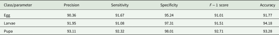
Table 3 shows the performance of Inception-v3 on test dataset. It is observed that the model performed better in classifying cells containing larvae with accuracy = 94.80%, specificity = 97.63%, sensitivity = 90.70% and F − 1 score = 92.03% and pupa with accuracy = 94.12%, specificity = 98.11%, sensitivity = 92.49% and F − 1 score = 93.05%. However, many of the egg cells were misclassified as larvae due to the unwanted illumination effects that appeared in egg cells. Thus the model performed least accurately when classifying cells containing eggs, with 92.03% accuracy, 96.85% specificity and 90.02% sensitivity. Since there are fewer parameters in Inception-v3 model compared to Inception-ResNet-v2, cell detection and classification is faster in Inception-v3.
Table 3. Performance measures using Inception-v3
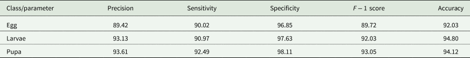
Table 4 represents the output performed on the proposed enhanced Inception-v3. The cells containing pupa have the maximum cell classification accuracy (CCA) of 95.22%, specificity = 98.26%, sensitivity = 93.24% and F − 1 score = 93.11%. However, few pupae are misclassified as larvae despite having similar texture. The cells containing eggs had the least precision, specificity and accuracy of 93.16, 97.31, and 92.86% respectively. The reason is that most of the egg cells were misclassified due to wax residuals inside the cells. Compared to other models the enhanced Inception-V3 model is best in detecting cells containing eggs.
Table 4. Performance measures using proposed enhanced Inception-v3
Discussion
Precision beekeeping is an approach that leverages advanced technologies and data-driven techniques to enable beekeepers to optimise hive management, detect disease early, enhance colony health, productivity and make informed decision based on data analysis. Traditional beekeeping techniques for estimating colony strength and health not only requires trained and skilled beekeepers but are also time-consuming due to their reliance on visual estimation which often lead to variability and erroneous observations.
In this paper, a computer vision based automated precision beekeeping system to analyse beehive cells for monitoring brood development stages is presented. The research was conducted with 62 beehive images in three fundamental steps: feature enhancement using a preprocessing pipeline, image segmentation and cell identification, and classification using transfer learning techniques.
During the experiment, it was observed that detecting the beehive cells correctly was the most challenging task due to their tiny size and thin cell boundaries. Thus, to enhance the visibility and interpretability of feature contained cell, the hive image is preprocessed with frequency domain denoising technique followed by contrast enhancement.
Further, segmentation and cell localisation was performed on processed images using CNN and CHT technique. Using a CNN to segment the comb was a reliable method as it produced an excellent result on captured images. However, it has been noted that CNN encountered challenges in segmenting the cells were still in the process of development or having irregular shapes. The findings indicate that the suggested model had achieved cell detection accuracy greater than ninety-seven per cent (fig. 5). The cells that were not capped were identified with a precision rate greater than ninety-eight per cent. The reason behind this is that the inner region of uncapped cells is darker and it appears as a hole which makes it easier to identify. However, capped cells were detected with lesser accuracy compared to uncapped cells because they contained honey which distorted cell boundaries, making them unidentifiable and increases the false negative detections.
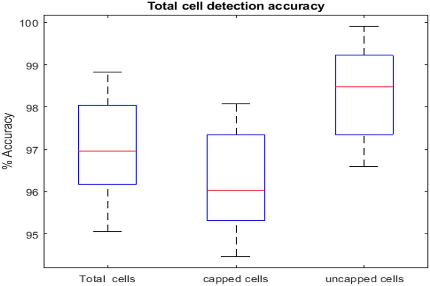
Figure 5. Comparison between total cell, capped cells, and uncapped cells detection accuracy.
Further, the detected cells were classified for three immature stages of bee brood (egg, larvae, and pupa) with three different models and their results were compared. In this work, pretrained CNNs of Inception-Resnet-v2, Inception-V3 and enhanced Inception-V3 that were trained on ImageNet database, were used for cell classification. The analysis conducted in the study comprehensively assessed several parameters, including CCA (Cell classification accuracy), Precision, Sensitivity, Specificity, and F1 score, to evaluate their impact on the model's performance and the effectiveness of the proposed methodology. During experimentation, we were able to identify and categorise the cells containing brood at various phases of development (fig. 6). The average accuracy attained for the overall detection of brood was 94.23%. The results of the study indicate that the proposed methodology achieved highest accuracy in discerning pupa and larvae cells in comparison to egg cells due to their distinctive texture and visual attributes. However, few very small larvae were misclassified as egg. Furthermore, certain cells have been observed to be infected with sac brood and chalk brood diseases. These cells are erroneously categorised as capped cells or pupa. Based on the findings, it can be inferred that the incorporation of deep learning models and the subsequent identification of robust features for optimal classification in the proposed enhanced Inception V3 model has resulted in an enhancement of the accuracy of cell categorisation.
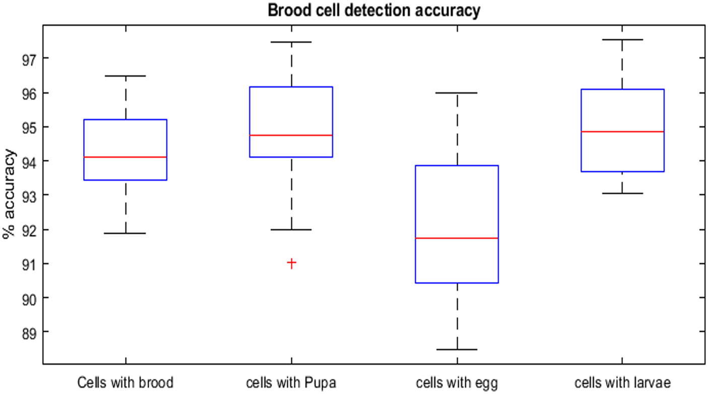
Figure 6. Comparison of brood detection accuracy.
Table 5 tabulates the comparison of proposed method with method suggested by Liew et al. (Reference Liew, Lee and Chan2010), Hoferlin et al. (Reference Hoferlin, Hoferlin, Kleinhenz and Bargen2013) and Paolillo et al. (Reference Paolillo, Petrini, Casiraghi, De Iorio, Biffani, Pagnacco, Minozzi and Valentini2022). All authors have performed manual segmentation which is not feasible as it is time consuming and affects the speed of detection The method described by Paolillo et al. (Reference Paolillo, Petrini, Casiraghi, De Iorio, Biffani, Pagnacco, Minozzi and Valentini2022) employs thresholding and the CHT technique to identify uncapped cells and evaluate hygienic behaviour. In comparison, our technique has demonstrated a 21.78% improvement in cell detection. Liew et al. (Reference Liew, Lee and Chan2010) suggested method utilises canny edge detection technique for the detection of cell boundaries. The obtained accuracy of 70.48% was attributed to the limitations of their method in detecting capped cells, caused due to presence of deformed edges. In contrast, our methodology successfully identified cells with a precision rate of 97.03%, hence providing reliable information regarding the presence of capped and uncapped cells within the frame.
Table 5. Comparison of proposed methodology with the existing methods
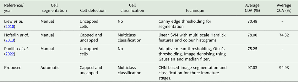
Hoferlin et al. (Reference Hoferlin, Hoferlin, Kleinhenz and Bargen2013) proposed approach utilises texture based segmentation and support vector machine for detection and classification of cells. Although, their method, successfully classifies the image, the overall accuracy is low compared to our method due to misinterpretation of cell containing wax and pollen with larvae and egg resulting in a large number of FPC. Since our method uses transfer leaning approach, the CNN models are able to detect fine detail resulting in more accurate classification.
Thus the proposed approach outperformed all existing methods and successfully accomplished the aim of developing a robust tool for analysis of beehive frame images. The aim of this research is the utilisation of process automation and implementation of tool equipped with machine learning and artificial intelligence in the field of apiculture to execute tasks that are on par with the capabilities of expert human workers. Through the integration of AI, beekeepers can achieve significant improvements in efficiency and accuracy. The images and parameters calculated are the permanent record that will be helpful for colony assessment. By analysing images captured by cameras placed inside the hives, it is possible to detect signs of disease or infestation, such as the presence of mites or abnormal behaviour in the bees. Beekeepers can utilise this information to proactively address disease transmission and uphold the well-being of their colonies. Additionally, the proposed method facilitates the enhancement of honey production by enabling beekeepers to closely observe hive conditions and bee behaviour. Beekeepers can achieve this by optimising the conditions within the hive, thereby ensuring the well-being and productivity of their bees. Keeping track on the brood development with automated precision beekeeping has significantly reduced the time of information collection and ensures beekeepers reliability and accuracy of brood status. During the experimentation, it is observed that there a few cells which contains both egg and larvae in one cell. The proposed method lacks in classifying those cells. However, such cells can be detected with the post processing.
The possibility of implementation of the algorithm in the MobileNet Network is in testing phase currently. MobileNet is a neural network architecture specifically developed to enable efficient image classification on mobile and embedded devices that possess restricted computational resources. It is specifically engineered to possess a compact form and expedite inference by incorporating a limited number of parameters in comparison to alternative classification networks. This feature makes it highly suitable for mobile and embedded devices that have limited computational resources. Furthermore, MobileNet has been specifically optimised to achieve efficient inference, enabling it to rapidly classify images while maintaining minimal latency. After enhancing the reported accuracy on MobileNet, it will be made available to the practitioners for real time analysis.
Data
The dataset used to build and analyse the resulting models are publicly available on the following link: (https://github.com/AvsThiago/DeepBee-source/archive/release-0.1.zip).
Author's contributions
Conceptualisation and methodology Neha Rathore and Dheeraj Agrawal; software, validation, formal analysis, investigation, data curation, writing – original draft preparation, Neha Rathore writing – review and editing, supervision, resources, Dheeraj Agrawal.
Financial support
This study was not funded by anyone.
Competing interests
I am herewith submitting the documents related to the manuscript entitled ‘Automated precision beekeeping for accessing bee brood development and behaviour using deep CNN’ for peer review. All the authors are hereby declaring that they have no known competing financial interests or personal relationships that could have appeared to influence the work reported in this paper.
Ethical standards
This article does not contain any studies with human participants or animals performed by any of the authors.


