


1. Introduction
We consider the compressible Navier–Stokes equations governing the motion of a fluid in some bounded domain $\Omega \subset \mathbb {R}^3$ , where we additionally insert a simply connected compact obstacle $\mathcal {B} \subset \mathbb {R}^3$
 . Denoting $\mathcal {F} = \Omega \setminus \mathcal {B}$
 the fluid's domain, the equations take the form
Here, $\rho$ and $\mathbf {u}$
 denote the fluid's density and velocity, respectively, $p$
 is the fluid's pressure given by $p(\rho )=\rho ^\gamma$
 for some $\gamma > 3/2$
 , $\mathbb {S}$
 the (viscous) stress tensor and $\mathbf {f} \in L^\infty ((0,\,T) \times \Omega )$
 a given external force density. Furthermore, $\rho _\mathcal {B}$
 is the solid's density, $\mathbf {G}$
 the centre of mass of the body $\mathcal {B}$
 , $\omega$
 its rotational velocity, $m>0$
 the object's mass given by
and $\mathbb {J}$ is the inertial tensor (moment of inertia) given by
The question of whether or not a solid body collides with its container has been addressed by several authors. Without claiming completeness, we refer to [Reference Gérard-Varet and Hillairet9–Reference Jin, Nečasová, Oschmann and Roy14] for recent results in this direction. The aim of this short note is to generalize these results to non-Newtonian fluids, as well as to heat-conducting fluids with temperature-growing viscosities. Lastly, let us also mention the related, though different, work [Reference Feireisl and Nečasová6], where the authors considered a so-called $k$ - or multi-polar compressible fluid, and showed that collisions do not occur for $k\geq 3$
 since the velocity and, accordingly, the density enjoy higher regularity. Together with the no-collision results given in the references above, this can be roughly summarized as ‘high regularity forbids collision’.
Notations:. Lebesgue and Sobolev spaces will be denoted in the usual way as $L^p(\Omega )$ and $W^{1,p}(\Omega )$
 , respectively. We will also denote them for vector- and matrix-valued functions as in the scalar case, that is, $L^p(\Omega )$
 instead of $L^p(\Omega ; \mathbb {R}^3)$
 . The Sobolev space of trace-zero functions will be denoted by $W_0^{1,p}(\Omega )$
 . For each $\mathbb {A},\,\mathbb {B} \in \mathbb {R}^{3 \times 3}$
 , we set the Frobenius inner product $\mathbb {A}: \mathbb {B} = \sum _{i,j=1}^3 A_{ij} B_{ij}$
 . Further, we define the Frobenius norm by $|\mathbb {A}|^2 = \mathbb {A} : \mathbb {A}$
 . To lean the notation, we will write $a \lesssim b$
 if there is a generic constant $C>0$
 which is independent of $a$
 , $b$
, $b$ , and the variables of interest such that $a \leq C b$
 . The constant might change its value wherever it occurs. The domains occupied by the solid and fluid at time $t \geq 0$
 are denoted by $\mathcal {B}(t)$
 and $\mathcal {F}(t)=\Omega \setminus \mathcal {B}(t)$
 , respectively.
2. General assumptions
Let us start by making precise the assumptions on the fluid and solid. First, the stress tensor $\mathbb {S}$ will depend on the symmetrized velocity gradient $\mathbb {D}(\mathbf {u})=1/2 ( \nabla \mathbf {u} + \nabla ^T \mathbf {u})$
 in a way described in (S1)–(S3) below. Second, we assume that the solid is homogeneous with constant mass density $\rho _\mathcal {B}>0$
 . The mass and centre of mass of the rigid body are given by
We will also assume that the solid's mass is independent of time, that is, $m=\rho _\mathcal {B} |\mathcal {B}(t)|$ for any $t\geq 0$
 , leading to the density-independent expression $\mathbf {G}(t) = |\mathcal {B}(t)|^{-1} \int _{\mathcal {B}(t)} x \ \mathrm {d} x$
 .
.
2.1. The stress tensor and uniform bounds
The crucial part in analysing collisions is to investigate the form of the stress tensor $\mathbb {S}$ . We will make the following assumptions:
(S1) Continuity: $\mathbb {S}$
 is a continuous mapping from $\mathbb {R}_{\rm sym}^{3\times 3}$ to itself depending only on the symmetric gradient $\mathbb {D}(\mathbf {u}) = 1/2 (\nabla \mathbf {u} + \nabla ^T \mathbf {u}) \in \mathbb {R}_{\rm sym}^{3 \times 3}$.
(S2) Monotonicity: For any $\mathbb {M},\, \mathbb {N} \in \mathbb {R}_{\rm sym}^{3 \times 3}$
, we have $[\mathbb {S}(\mathbb {M}) - \mathbb {S}(\mathbb {N})] : (\mathbb {M} - \mathbb {N}) \geq 0$.(S3) Growth: There are absolute constants $\delta \geq 0$
and $0< c_0\leq c_1<\infty$ such that for some $p>1$ and all $\mathbb {M} \in \mathbb {R}_{\rm sym}^{3\times 3}$, we have $c_0 |\mathbb {M}|^p - \delta \leq \mathbb {S}(\mathbb {M}):\mathbb {M} \leq c_1 |\mathbb {M}|^p$.


We note that classical power-law fluids like $\mathbb {S} = |\mathbb {D}(\mathbf {u})|^{p-2} \mathbb {D}(\mathbf {u})$ , but also so-called activated Euler fluids with $\mathbb {S}=\max \{|\mathbb {D}(\mathbf {u})|-\delta _0,\, 0\}|\mathbb {D}(\mathbf {u})|^{-1} \mathbb {D}(\mathbf {u})$
 for some $\delta _0>0$
 fit into this setting. In contrast to the fact that we do not consider temperature in here, we will give another example of temperature-growing viscosities in § 4. Note moreover that condition (S3) implies by duality $\mathbb {S} \in L^{p'}((0,\,T)\times \Omega )$
 since
since
Remark 2.1 We remark that the question of existence of a weak solution to problem (1.1) is just solved in some special cases, see [Reference Feireisl3] for Newtonian fluids, and [Reference Feireisl, Liao and Malek5] for a special non-Newtonian fluid with bounded divergence of the velocity. On the other hand, for non-Newtonian incompressible fluids, existence is shown in [Reference Feireisl, Hillairet and Nečasová4], and in [Reference Nečasová15] for incompressible heat-conducting fluids. In those two existence results, collisions cannot occur due to a high regularity of the velocity, in particular, $p \geq 4$ there.
To start analysing the collision behaviour, one first needs uniform bounds on the velocity and density. With a slight abuse of notation, we extend the velocity and density as
Noticing that the energy inequality obtained in [Reference Feireisl, Liao and Malek5] implies in our case

for almost any $\tau \in [0,\,T]$ , an immediate consequence is the uniform estimate

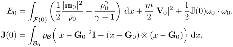
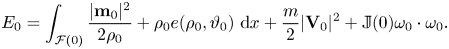
Here, $E_0$ is the initial energy of the system given by
and the ‘$+1$ ’ on the right-hand side of (2.2) is a sole remainder of the force $\mathbf {f}$
 on the right-hand side of (1.1)$_2$
 . Moreover, the implicit constant appearing in (2.2) is independent of the mass $m$
 and the final time $T$
 .
.
We remark that such bounds also hold true for other models of non-Newtonian fluids such as dissipative (measure-valued) solutions, see [Reference Abbatiello and Feireisl1]. However, the additional Reynolds stress appearing in the momentum equation for such type of solutions is not regular enough for our purposes, in particular, we need to work with weak solutions rather than dissipative ones. Since the present work does not focus on existence of weak solutions, for the definition of such we refer the reader to [Reference Feireisl, Liao and Malek5].
2.2. The solid's shape and main result
Throughout the paper, we consider a $C^{1,\alpha }$ solid moving vertically over a flat horizontal surface under the influence of gravity. More precisely, we make the following assumptions (see figure 1 for the main notations):
(A1) The source term is provided by the gravitational force ${\mathbf {f}}=-g{\mathbf {e}}_3$
and $g>0$.(A2) The solid moves along and is symmetric to the $x_3$
-axis $\{x_1=x_2=0\}$.(A3) The only possible collision point is at $x=0 \in \partial \Omega$
, and the solid's motion is a vertical translation.(A4) Near $r=0$
, $\partial \Omega$ is flat and horizontal, where $r=\sqrt {x_1^2+x_2^2}$.(A5) Near $r=0$
, the lower part of $\partial \mathcal {B}(t)$ is given by
\[ x_3={ h(t)+r^{1+\alpha}},\ r\leq 2r_0\text{ for some small enough } r_0>0. \]
(A6) The collision just happens near the flat boundary of $\Omega$
:
\[ \inf_{t > 0}{\rm dist} \left(\mathcal{B}(t),\partial\Omega \setminus [{-}2r_0, 2r_0]^2\times\{0\}\right)\geq d_0>0. \]


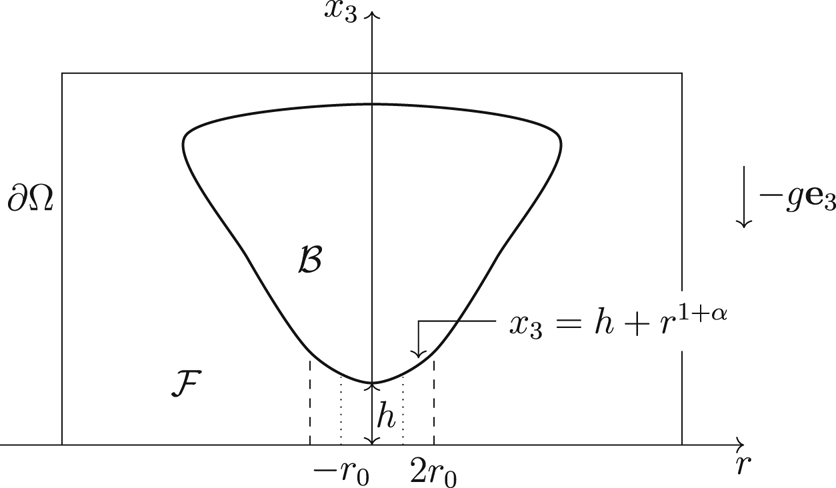
Figure 1. The body $\mathcal {B}$ and fluid $\mathcal {F}$
 in the container $\Omega$
 .
.
By (A2) and (A3), we may additionally assume that the position of the solid is characterized by its height $h(t)$ , in the sense that

Note especially that this means that the solid rotates at most around the $x_3$ -axis, and so $\omega (t) = \pm |\omega (t)| \mathbf {e}_3$
 . This assumption can be made rigorous for Newtonian incompressible fluids and symmetric initial data in 2D, see [Reference Gérard-Varet and Hillairet9].
Our main result regarding collision now reads as follows:
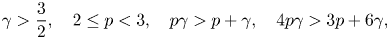
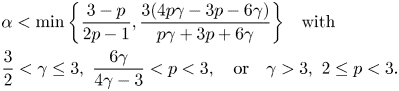
Theorem 2.2 Let $\gamma >{3}/{2}$ , $2 \leq p < 3$
 , $0<\alpha \leq 1$
 , and $\Omega,\,\ \mathcal {B}\subset \mathbb {R}^3$
 be bounded domains of class $C^{1,\alpha }$
 . Let $(\rho,\, \mathbf {u},\, {\mathbf {G}})$
 be a weak solution to (1.1) enjoying the bounds (2.2), let $\mathbb {S}$
 comply with (S1)–(S3) and assume that (A1)–(A6) are fulfilled. If the solid's mass is large enough, and its initial vertical and rotational velocities are small enough, then the solid touches $\partial \Omega$
 in finite time provided

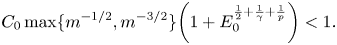
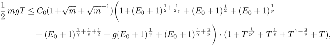
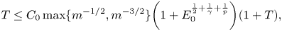
Remark 2.3 The terms ‘large enough’ and ‘small enough’ should be interpreted in such a way that inequality (3.8) is satisfied. More precisely, for some constant $C_0>0$ which is independent of $m$
 and $T$
 , we ensure collision provided
Remark 2.4 Let us mention a few facts about the above constraints. First, the two expressions inside the minimum stem, as one shall expect, from estimating the diffusive and convective part, respectively.
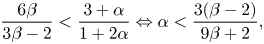
Second, the restriction $p<3$ is due to the diffusive part, see the estimate of $I_4$
 in § 3.2. Moreover, the requirement $p\geq 2$
 stems from the convective term, since we need to estimate the square of the velocity in time. Thus, our result as stated above is just valid for shear-thickening fluids. Omitting convection, theorem 2.2 still holds provided

hence also allowing for shear-shinning fluids if $\gamma >2$ .
.
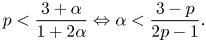
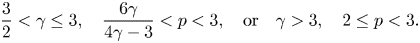
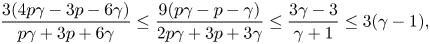
Third, the first condition on $p$ and $\gamma$
 in (2.4) can be equivalently stated as ${3p}/{(4p-6)} < \gamma \leq 3$
 , $2< p<3$
 .
.
Lastly, the first fraction inside the minimum in (2.4) wins precisely if $\gamma \geq {3p}/{(5p-9)}$ , and in (2.5) if $\gamma \geq {3p}/{(4p-6)}$
 . This seems to be optimal in the sense that for $p=2$
 , $\alpha =1/3$
 is a ‘borderline value’ for the incompressible case, which would (loosely speaking) correspond to $\gamma =\infty$
 (see [Reference Gérard-Varet and Hillairet10, Section 3.1] for details). Moreover, the assumptions in (2.4) coincide with the requirements on $\alpha$
 and $\gamma$
 made in [Reference Jin, Nečasová, Oschmann and Roy14], where the compressible Newtonian case (corresponding to $p=2$
 ) was considered.
Remark 2.5 As will be immediate from the calculations, the same conclusion holds for non-Newtonian heat-conducting fluids such that assumptions (S1)–(S3) are replaced by
(S1’) Continuity: $\mathbb {S}$
is a continuous mapping from $(0,\,\infty ) \times \mathbb {R}_{\rm sym}^{3\times 3}$ to $\mathbb {R}_{\rm sym}^{3 \times 3}$ depending continuously on the temperature $\vartheta >0$ and the symmetric gradient $\mathbb {D}(\mathbf {u}) = 1/2 (\nabla \mathbf {u} + \nabla ^T \mathbf {u}) \in \mathbb {R}_{\rm sym}^{3 \times 3}$.(S2’) Monotonicity: For any $\vartheta \in (0,\,\infty )$
and any $\mathbb {M},\, \mathbb {N} \in \mathbb {R}_{\rm sym}^{3 \times 3}$, we have $[\mathbb {S}(\vartheta,\, \mathbb {M}) - \mathbb {S}(\vartheta,\, \mathbb {N})] : (\mathbb {M} - \mathbb {N}) \geq 0$.(S3’) Growth: There are absolute constants $\delta \geq 0$
and $0< c_0\leq c_1<\infty$ such that for some $p>1$, all $\vartheta >0$, and all $\mathbb {M} \in \mathbb {R}_{\rm sym}^{3\times 3}$, we have $c_0 |\mathbb {M}|^p - \delta \leq \mathbb {S}(\vartheta,\, \mathbb {M}):\mathbb {M} \leq c_1 |\mathbb {M}|^p$.


3. Construction of test function and proof of main result
In this section, we will define an appropriate test function for the momentum equation that will ensure collision. Let $(\rho,\, \mathbf {u},\, {\mathbf {G}})$ be a weak solution of (1.1) satisfying assumptions (A1)–(A6) in the time interval $(0,\,T_*)$
 before collision and enjoying the bounds (2.2). From now on we denote $\mathcal {B}_h=\mathcal {B}_h(t)=\mathcal {B}(0)+(h(t)-h(0)){\mathbf {e}}_3$
 and $\mathcal {F}_{h}=\mathcal {F}_h(t)=\Omega \setminus \mathcal {B}_h(t)$
 . As mentioned before, the assumption on $\mathcal {B}(t)$
 especially means that the whole configuration is cylindrically symmetric with respect to the $x_3$
 -axis.
Collision can occur if and only if $\lim _{t\to T_*}h(t)=0$ . Note further that ${\rm dist}(\mathcal {B}_h(t),\,\partial \Omega )= \min \{h(t),\,d_0\}$
 by assumptions (A2) and (A6).
3.1. Test function
We will make use of cylindrical coordinates $(r,\,\theta,\,x_3)$ with the standard basis $(\mathbf {e}_r,\, \mathbf {e}_\theta,\, \mathbf {e}_3)$
 . We take the same function as in [Reference Gérard-Varet and Hillairet10] (see also [Reference Gérard-Varet and Hillairet9, Reference Gérard-Varet, Hillairet and Wang12]), which is constructed as a function ${\mathbf {w}}_h$
 associated with the solid particle $\mathcal {B}_h$
 frozen at distance $h$
 . This function will be defined for $h\in (0,\,\sup _{t\in [0,T_*)}h(t))$
 . We see that when $h\to 0$
 , a cusp arises in $\mathcal {F}_h$
 , which is contained in

For the sequel, we fix $h$ as a (small) positive constant and define $\psi (r):= h+r^{1+\alpha }$
 . Note that the common boundary $\partial \Omega _{h,r_0}\cap \partial \mathcal {B}_h$
 is precisely given by the set $\{0\leq r\leq r_0,\,\ x_3=\psi (r)\}$
 .
.
Let us derive how an appropriate test function inside $\Omega _{h, r_0}$ might look like. In order to get rid of the pressure term, we seek for a function $\mathbf {w}_h$
 which is divergence-free. Additionally, it shall be rigid on $\mathcal {B}_h$
 , and comply with its motion. Thus, our test function shall satisfy

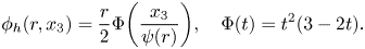
hence we choose $\mathbf {w}_h = \nabla \times (\phi _h \mathbf {e}_\theta )$ for some function $\phi _h(r,\,x_3)$
 to be determined. In cylindrical coordinates, we write $\mathbf {w}_h$
 as
as
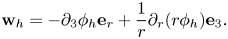
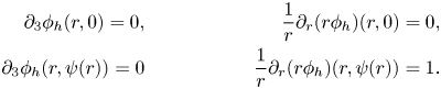
The boundary conditions on $\mathbf {w}_h$ translate for $\phi _h$
 into
into
Further, considering the energy
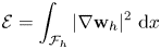
and anticipating that most of it stems from the vertical motion, that is, from the derivative in $x_3$ -direction, we get
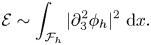
The Euler–Lagrange equation for the functional $\mathcal {E}$ thus reads $\partial _3^4 \phi _h(r,\, x_3)=0$
 . A simple calculation now leads to the general form

In order to get a smooth bounded function $\phi _h$ for all values of $r$
 and $x_3$
 , we choose $\kappa _1=\kappa _2=0$
 to infer
Hence, inside $\Omega _{h, r_0}$ , the so constructed function will take advantage of the precise form of the solid. Extending $\phi _h$
 in a proper way, we thus can define a proper test function $\mathbf {w}_h$
 defined in the whole of $\Omega$
 .
.
To achieve this, we use a similar method as in [Reference Gérard-Varet and Hillairet9]: define smooth functions $\chi,\, \eta$ satisfying

where $d_0>0$ is as in (A6), and $\mathcal {N}_\delta$
 is a $\delta$
 -neighbourhood of $\mathcal {B}(0)$
 . With a slight abuse of notation for $\phi _h$
 , set
, set

and $\mathbf {w}_h = \nabla \times (\phi _h \mathbf {e}_\theta )$ . Observe that the function $\mathbf {w}_h$
 satisfies

Indeed, the divergence-free condition is obvious from the definition of $\mathbf {w}_h$ . Further, since $\phi _h = r/2$
 on $\mathcal {B}_h$
 , we have $\mathbf {w}_h = \mathbf {e}_3$
 there. Moreover, by definition of $\chi$
 and $\eta$
 , we have $\phi _h=0$
 on $\partial \Omega \setminus ( (-2 r_0,\, 2 r_0)^2 \times \{ 0 \} )$
 as long as $r_0$
 and $h$
 are so small that $h+r_0^{1+\alpha } \leq d_0 < r_0$
 . Lastly, $\phi _h=0$
 on $\partial \Omega \cap (-r_0,\, r_0)^2 \times \{0\}$
 by definition of $\chi$
 and $\Phi (0)=0$
 , and in the annulus $( (-2r_0,\, 2r_0)^2 \setminus (-r_0,\, r_0)^2 ) \times \{ 0 \}$
 we use also $\eta (r,\,h(0))=0$
 for $r>\mathfrak {r}_0$
 for some $\mathfrak {r}_0\in (d_0,\, r_0)$
 to finally conclude $\mathbf {w}_h|_{\partial \Omega }=0$
 , provided $h$
 is sufficiently close to zero.
We summarize further properties in the following lemma, the proof of which is given in [Reference Jin, Nečasová, Oschmann and Roy14, Lemma 3.1]:
Lemma 3.1 $\mathbf {w}_h\in C_c^\infty (\Omega )$ and
and

Moreover,
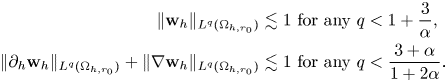
Remark 3.2 The condition $\alpha (q-1)<3$ coming from $\mathbf {w}_h$
 is consistent with the results of [Reference Starovoitov16], where the author showed that collision is forbidden as long as $\alpha (q-1) \geq 3$
 . Especially, for shapes of class $C^{1,1}$
 like balls, this states that no collision can occur as long as $q \geq 4$
 , which fits the assumptions made in [Reference Feireisl, Hillairet and Nečasová4] and [Reference Nečasová15]. Moreover, the difference $q - \frac{2+\alpha }{1+2\alpha }$
 occurs in the incompressible two-dimensional setting in [Reference Filippas and Tersenov8, Theorem 3.2] as an optimal value for the solid to move vertically; our fraction $\frac{3+\alpha }{1+2\alpha }$
 thus seems like a three-dimensional counterpart to this.
3.2. Estimates near the collision—proof of theorem 2.2
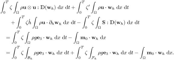
Let $0< T< T_*$ and let $\zeta \in C^1_c([0,\,T))$
 with $0\leq \zeta \leq 1$
 , $\zeta '\leq 0$
 , and $\zeta =1$
 near $t=0$
 . We take $\zeta (t){\mathbf {w}}_{h(t)}$
 as test function in the weak formulation of the momentum equation (1.1)$_2$
 with right-hand side ${\mathbf {f}}=-g{\mathbf {e}}_3$
 , $g>0$
 . Recalling $\operatorname {\mathrm {div}}\mathbf {w}_h=0$
 and $\partial _t \mathbf {w}_{h(t)}=\dot {h}(t) \partial _h\mathbf {w}_{h(t)}$
 , we get
Observe that we have $\mathbf {w}_h=\mathbf {e}_3$ on $\mathcal {B}_h$
 , so for a sequence $\zeta _k\to 1$
 in $L^1([0,\,T))$
 ,
,

In particular, for a proper choice of $\zeta$ , it follows that
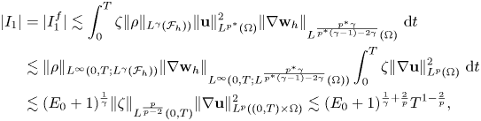
We will estimate each $I_j$ separately, and set our focus on the explicit dependence on $T$
 and $m$
 . For the latter purpose, we split each density-dependent integral into its fluid and solid part $I_j^f$
 and $I_j^\mathcal {B}$
 , respectively. The proof follows the same lines as [Reference Jin, Nečasová, Oschmann and Roy14], so we will just state the estimates and highlight the differences due to the non-Newtonian setting.
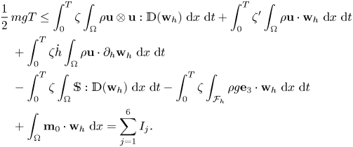
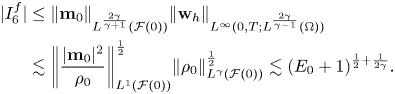
$\bullet$ For $I_2^f$
 , we have
$\bullet$ For $I_2^\mathcal {B}$
 , note that due to $\omega (t) = \pm |\omega (t)| \mathbf {e}_3$
 , $\mathbf {u} |_{\mathcal {B}_h} = \dot {\mathbf {G}}(t) + \omega \times (x - \mathbf {G}(t))$
 , $\mathbf {G}(t) = \mathbf {G}(0) + (h(t)-h(0))\mathbf {e}_3$
 , $\rho |_{\mathcal {B}_h} = \rho _\mathcal {B}>0$
 , and $\mathbf {w}_h |_{\mathcal {B}_h} = \mathbf {e}_3$
 , we have

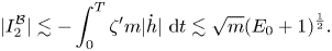
Further, from the bounds (2.2), we infer

Hence, by the choice of $\zeta$ such that $|\zeta '|=-\zeta '$
 and $\zeta (0)=1+\zeta (T)=1$
 , we get
$\bullet$ For $I_3$
 , observe that $I_3^\mathcal {B}=0$
 due to $\partial _h \mathbf {w}_h|_{\mathcal {B}_h} = \partial _h \mathbf {e}_3=0$
 . Next, by Sobolev embedding and the bounds (2.2),

where we set $p^\ast = 3p/(3-p)$ . Thus,
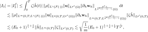
where we have used estimate (2.2) and lemma 3.1 under the condition

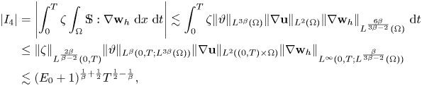
$\bullet$ Regarding $I_4$
 , using that $\mathbb {S} \in L^{p'}((0,\,T) \times \Omega )$
 is bounded by $c_1>0$
 (see (2.1)), we calculate
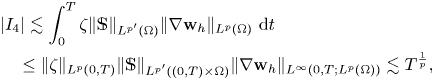
where we have used lemma 3.1 under the condition
From here, we get the restriction $p<3$ .
.
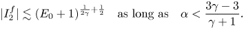
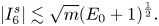
$\bullet$ For $I_5=I_5^f$
 ,
,

$\bullet$ Similar to $I_2^f$
 , we have for $I_6^f$
$\bullet$ For $I_6^\mathcal {B}$
 , since $\mathbf {m}_0\cdot \mathbf {w}_h |_{\mathcal {B}_h} = \rho _\mathcal {B} \mathbf {u}(0)|_{\mathcal {B}_h} \cdot \mathbf {e}_3 = \rho _\mathcal {B} \dot h$
 ,
,
$\bullet$ Let us turn to $I_1$
 . Due to $\mathbf {w}_h|_{\mathcal {B}_h}=\mathbf {e}_3$
 , we see that $I_1^\mathcal {B}=0$
 since $\mathbb {D}(\mathbf {w}_h)=0$
 there. Hence, we calculate
by using estimate (2.2) and lemma 3.1 under the condition

Let us emphasize that this term is the only place where the assumption $p\geq 2$ is needed.
Collecting all the requirements made above, we infer
which translates into
Note further that for any $\gamma \geq 3/2$ and any ${\gamma }/{(\gamma -1)}< p<3$
 ,
,
and that all estimates are independent of the choice of $\zeta$ . Hence, we can take a sequence $\zeta _k\to 1$
 in $L^r([0,\,T))$
 for some suitable $r > 1$
 without changing the bounds obtained. In turn, collecting all estimates above, we finally arrive at
which, after dividing by $\frac{1}{2} {mg}$ and using Young's inequality on several terms, leads to
where $C_0$ only depends on $p,\, \gamma,\, g,\, \alpha$
 , the bounds on $\mathbf {w}_h$
 obtained in lemma 3.1, and the implicit constant appearing in (2.2), provided
Recalling the definition of $E_0$ from (2.3) as
we see that collision can occur only if the solid's mass in (3.7) is large enough, meaning in fact its density is very high. Since $E_0$ depends on the solid's mass, we require the solid initially to have low vertical and rotational speed. More precisely, choosing $\mathbf {V}_0$
 and $\omega _0$
 such that $|\mathbf {V}_0|,\, |\omega _0|=\mathcal {O}(m^{-1/2})$
 , and choosing $m$
 high enough such that

the solid touches the boundary of $\Omega$ in finite time, finishing the proof of theorem 2.2.
Remark 3.3 We see that if, by change, the constant $C_0<1$ small enough, then we can get rid of the assumption on the smallness of $\mathbf {V}_0$
 and $\omega _0$
 by also choosing $m<1$
 . Indeed, in this case $\max \{m^{-1/2},\, m^{-3/2} \} = m^{-3/2}$
 and $E_0 \lesssim 1$
 . Hence, for appropriate values $m<1$
 and $C_0 m^{-3/2} < 1$
 , inequality (3.8) can still be valid.
4. Newtonian flow with temperature-growing viscosity
This section is devoted to investigate a different model for viscosity that does not fit into assumptions (S1)–(S3). More precisely, let
where the viscosity coefficients $\mu,\,\eta$ are assumed to be continuous functions on $(0,\,\infty )$
 , $\mu$
 is moreover Lipschitz continuous, and they satisfy

Note that this means we consider a Newtonian fluid with growing viscosities that are not uniformly bounded in the temperature variable.
The equations governing the fluid's motion are now given by
where now $p(\rho,\, \vartheta ) = \rho ^\gamma + \rho \vartheta + \vartheta ^4$ , the heat flow vector $\mathbf {q} = \mathbf {q}(\vartheta,\, \nabla \vartheta )$
 is given by Fourier's law
with the heat conductivity coefficient satisfying
and the specific entropy $s=s(\rho,\, \vartheta )$ is connected to the pressure $p(\rho,\, \vartheta )$
 and the internal energy $e(\rho,\, \vartheta )$
 of the fluid by Gibbs’ relation
Note that this relation determines the internal energy and specific entropy as
where $c_v>0$ is the specific heat capacity at constant volume (see, e.g., [Reference Feireisl and Novotný7]). Denoting $\vartheta _\mathcal {B}>0$
 the solid's temperature, we extend the temperature similarly to the velocity and density as
and we consider the continuity of the heat flux $\mathbf {q}(\vartheta,\, \nabla \vartheta )\cdot \mathbf {n} = \mathbf {q}(\vartheta _\mathcal {B},\, \nabla \vartheta _\mathcal {B}) \cdot \mathbf {n}$ on $\partial \mathcal {B}$
 . Moreover, for simplicity we assume that the heat conductivity coefficient of the solid is the same as the fluid's one (this can be generalized, see [Reference Březina2, Equation (4.23)]).
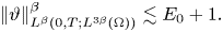
Noticing that the existence proof of theorem 4.1.6 in [Reference Březina2] also works for any $\beta >2$ instead of $\beta =3$
 , in such case we have the uniform bound
where this time
Thanks to Sobolev embedding, this yields

in turn,
Accordingly, the estimate for the stress tensor in $I_4$ changes into
provided
while all the other estimates stay the same. Hence, repeating the arguments from § 3, we can state the following
Theorem 4.1 Let $\gamma >3$ , $\beta >2$
 , $0<\alpha \leq 1$
 , and $\Omega,\, \mathcal {B}\subset \mathbb {R}^3$
 be bounded domains of class $C^{1,\alpha }$
 . Let $(\rho,\, \vartheta,\, \mathbf {u},\, {\mathbf {G}})$
 be a weak solution to (4.2) enjoying the bounds (2.2) and (4.4), with the initial energy given by (4.3). Moreover, let $\mathbb {S}$
 be given by (4.1), and assume that (A1)–(A6) are satisfied. If the solid's mass is large enough, and its initial vertical and rotational velocities are small enough such that inequality (3.8) is fulfilled, then the solid touches $\partial \Omega$
 in finite time provided
As can be easily seen, the same arguments can be used for temperature-dependent non-Newtonian fluids, provided the stress tensor decomposes like

for some tensor $\tilde {\mathbb {S}}$ satisfying (S1)–(S3), and $\mu,\, \eta$
 are as above. The details are left to the interested reader.
Remark 4.2 As a matter of fact, all the analyses in this article also hold for the incompressible case, which (roughly speaking) corresponds to $\gamma =\infty$ . Thus, collision for this type of heat-conducting fluids occurs if $\beta >2$
 and $\alpha <{3(\beta -2)}/{(9\beta +2)}$
 . Also here, for constant temperature corresponding to a perfectly heat-conducting fluid, we recover the borderline value $\alpha <1/3$
 in the limit $\beta \to \infty$
 , see remark 2.4.
Acknowledgements
Š. N. and F. O. have been supported by the Czech Science Foundation (GAČR) project 22-01591S. Moreover, Š. N. has been supported by Praemium Academiae of Š. Nečasová. The Institute of Mathematics, CAS is supported by RVO:67985840.


