Hostname: page-component-cd9895bd7-lnqnp Total loading time: 0 Render date: 2024-12-28T02:16:58.104Z Has data issue: false hasContentIssue false

Large-eddy simulation-based shape optimization for mitigating turbulent wakes of a bluff body using the regularized ensemble Kalman method

Published online by Cambridge University Press:  12 December 2024

Xin-Lei Zhang
Affiliation:
The State Key Laboratory of Nonlinear Mechanics, Institute of Mechanics, Chinese Academy of Sciences, Beijing 100049, PR China School of Engineering Sciences, University of Chinese Academy of Sciences, Beijing 100049, PR China
Fengshun Zhang
Affiliation:
The State Key Laboratory of Nonlinear Mechanics, Institute of Mechanics, Chinese Academy of Sciences, Beijing 100049, PR China School of Engineering Sciences, University of Chinese Academy of Sciences, Beijing 100049, PR China
Zhaobin Li
Affiliation:
The State Key Laboratory of Nonlinear Mechanics, Institute of Mechanics, Chinese Academy of Sciences, Beijing 100049, PR China School of Engineering Sciences, University of Chinese Academy of Sciences, Beijing 100049, PR China
Xiaolei Yang
Affiliation:
The State Key Laboratory of Nonlinear Mechanics, Institute of Mechanics, Chinese Academy of Sciences, Beijing 100049, PR China School of Engineering Sciences, University of Chinese Academy of Sciences, Beijing 100049, PR China
Guowei He*
Affiliation:
The State Key Laboratory of Nonlinear Mechanics, Institute of Mechanics, Chinese Academy of Sciences, Beijing 100049, PR China School of Engineering Sciences, University of Chinese Academy of Sciences, Beijing 100049, PR China
*
Email address for correspondence: [email protected]

Abstract

In this work, the shape of a bluff body is optimized to mitigate velocity fluctuations of turbulent wake flows based on large-eddy simulations (LES). The Reynolds-averaged Navier–Stokes method fails to capture velocity fluctuations, while direct numerical simulations are computationally prohibitive. This necessitates using the LES method for shape optimization given its scale-resolving capability and relatively affordable computational cost. However, using LES for optimization faces challenges in sensitivity estimation as the chaotic nature of turbulent flows can lead to the blowup of the conventional adjoint-based gradient. Here, we propose using the regularized ensemble Kalman method for the LES-based optimization. The method is a statistical optimization approach that uses the sample covariance between geometric parameters and LES predictions to estimate the model gradient, circumventing the blowup issue of the adjoint method for chaotic systems. Moreover, the method allows for the imposition of smoothness constraints with one additional regularization step. The ensemble-based gradient is first evaluated for the Lorenz system, demonstrating its accuracy in the gradient calculation of the chaotic problem. Further, with the proposed method, the cylinder is optimized to be an asymmetric oval, which significantly reduces turbulent kinetic energy and meander amplitudes in the wake flows. The spectral analysis methods are used to characterize the flow field around the optimized shape, identifying large-scale flow structures responsible for the reduction in velocity fluctuations. Furthermore, it is found that the velocity difference in the shear layer is decreased with the shape change, which alleviates the Kelvin–Helmholtz instability and the wake meandering.

Type
JFM Papers
Copyright
© The Author(s), 2024. Published by Cambridge University Press

1. Introduction

The turbulent wake of bluff bodies is a canonical flow that exists widely in engineering applications. The wake flows can produce unsteady loads on the bluff body due to boundary layer separation and vortex shedding (Patnaik & Wei Reference Patnaik and Wei2002; Choi, Jeon & Kim Reference Choi, Jeon and Kim2008; Rashidi, Hayatdavoodi & Esfahani Reference Rashidi, Hayatdavoodi and Esfahani2016). It not only causes severe structural vibration on the cylinder, but also generates significant turbulent noises from vortex evolution. Therefore, it is of practical interest to mitigate these detrimental effects from turbulent wakes.

Shape optimization is one extensively used passive control approach to mitigating turbulent wakes (Mohammadi & Pironneau Reference Mohammadi and Pironneau2009), without requiring extra energy inputs (Min & Choi Reference Min and Choi1999; Cattafesta & Sheplak Reference Cattafesta and Sheplak2011). It is often achieved with the adjoint-based approach that uses adjoint variables to characterize the gradient of objective functions and guide the optimization of geometric parameters. Specifically, the equation of the adjoint variables can be derived with integration by parts from the primal equation, e.g. the Reynolds-averaged Navier–Stokes (RANS) equation, and further solved to provide the gradient of the objective function with respect to the geometric parameters (Dhert, Ashuri & Martins Reference Dhert, Ashuri and Martins2017). However, the accuracy of the RANS method depends highly on the turbulence model, which often leads to large predictive discrepancies when encountered with flow separation, e.g. behind the bluff body, due to the model inadequacy (Xiao & Cinnella Reference Xiao and Cinnella2019). Moreover, the RANS-based shape optimization is not applicable for specific purposes associated with turbulent fluctuation, including turbulent wake mitigation. That is because the fluctuating information is lost with ensemble averaging in the RANS equation, and has to be modelled with empirical assumptions. For instance, the turbulent kinetic energy (TKE), characterized by root mean square of velocity fluctuations, is estimated by solving the corresponding transport equation, in which the dissipation rate term is constructed in an ad hoc manner. Hence the predicted TKE is often considered an operating parameter for the eddy viscosity estimation, intrinsically different from experimental measurements. For these reasons, scale-resolving simulations, e.g. large-eddy simulations (LES) and direct numerical simulations (DNS), are needed for shape optimization to mitigate the turbulent wake of bluff bodies. In this work, we focus on the LES-based method for the following reasons. On the one hand, LES can be performed at relatively low computational costs in contrast to DNS. On the other hand, LES can accurately predict velocity fluctuations by resolving spatiotemporal scales of turbulent flows (Bodony & Lele Reference Bodony and Lele2005; Zhu, Wu & He Reference Zhu, Wu and He2022), which is a necessity to construct the objective function for mitigating wake instability.

The difficulty in the LES-based shape optimization lies in the sensitivity analysis of the predicted turbulence statistics with respect to the geometric parameters. The conventional adjoint method often leads to local instability in the gradient solution for the LES-based optimization, due to the chaotic nature of turbulent flows (Lea, Allen & Haine Reference Lea, Allen and Haine2000; Blonigan et al. Reference Blonigan, Fernandez, Murman, Wang, Rigas and Magri2016). Specifically, the LES resolve various scales of flow structures, and capture the chaotic dynamics of turbulent flows with the well-known butterfly effects. That is, a small variation of the initial condition results in large changes in the LES predictions of instantaneous flow fields. This ill-conditioned issue can lead to the blowing up, i.e. divergence to infinity, in computing gradients of the long-time averaged model outputs, including the TKE. Besides, the adjoint-based sensitivity analysis can be limited by considerable storage requirements for solving unsteady adjoint equations (Mani & Mavriplis Reference Mani and Mavriplis2008), because the adjoint method requires the previously computed instantaneous flow fields to be available at each time step (Nadarajah & Jameson Reference Nadarajah and Jameson2007). This storage requirement can be alleviated by using dynamic checkpointing techniques (Wang, Moin & Iaccarino Reference Wang, Moin and Iaccarino2009). Nevertheless, the blowup issue still severely limits the utility of the adjoint method for chaotic systems, e.g. turbulent flows.

Various approaches have been introduced to address the difficulties of sensitivity analysis for chaotic systems. For instance, the least squares shadowing method (Wang, Hu & Blonigan Reference Wang, Hu and Blonigan2014) is proposed by regularizing the ill-posed inverse problem with the closest trajectory to a pre-specified reference one. Also, one can remedy the blowup gradient by taking sample averaging of adjoint sensitivity over short trajectories (Lea et al. Reference Lea, Allen and Haine2000; Ni & Wang Reference Ni and Wang2017). The feasibility of such an ensemble-averaged adjoint sensitivity has been demonstrated (Chandramoorthy et al. Reference Chandramoorthy, Fernandez, Talnikar and Wang2019) for chaotic systems that can provide reasonably accurate gradients but at a poor convergence rate. Besides, gradient-free methods, such as genetic programming and pattern search methods (Holst & Pulliam Reference Holst and Pulliam2001; Marsden et al. Reference Marsden, Wang, Dennis and Moin2007), have been introduced for chaotic problems to circumvent the difficulties of the adjoint methods. However, these methods would be computationally prohibitive to optimize high-dimensional geometrical parameters, compared to gradient-based approaches. Hence it is of significant interest to develop feasible gradient-based methods for LES-based shape optimization.

The stochastic approximation method (Lai Reference Lai2003) can provide numerical gradients of complex systems with random samples, which includes the Kiefer–Wolfowitz algorithm (Kiefer & Wolfowitz Reference Kiefer and Wolfowitz1952), the simultaneous perturbation stochastic approximation (SPSA) method (Spall Reference Spall1992), and ensemble-based sensitivity analysis (Ancell & Hakim Reference Ancell and Hakim2007; Torn & Hakim Reference Torn and Hakim2008), among others. These methods differ mainly in the sample numbers and the gradient approximation scheme. For instance, the Kiefer–Wolfowitz algorithm and the SPSA method estimate the model gradient in a finite difference scheme with only two samples. The difference between the two methods is that the Kiefer–Wolfowitz method draws samples by perturbing only one direction, while the SPSA method disturbs all directions simultaneously. In contrast, the ensemble-based sensitivity method draws multiple samples from a multivariate Gaussian distribution along all directions, and estimates the gradient with a linear regression formula. The ensemble-based method can be more robust for finding the gradient-descent direction than other gradient approximation methods (Chen, Oliver & Zhang Reference Chen, Oliver and Zhang2009; Li & Reynolds Reference Li and Reynolds2011; Michelén-Ströfer, Zhang & Xiao Reference Michelén-Ströfer, Zhang and Xiao2021b).

Ensemble-based sensitivity analysis (Ancell & Hakim Reference Ancell and Hakim2007) has been employed for gradient approximation of chaotic systems. The method estimates model gradients from the statistical perspective, in stark contrast to the adjoint method, which derives the gradient from the dynamic perspective. Specifically, the adjoint method solves the dynamical equation, i.e. the adjoint equation, to estimate the gradient information, while the ensemble method uses the sample covariance of the model inputs and time-averaged outputs to achieve this goal. In doing so, the statistics of chaotic solutions are used to characterize the model gradient, which can vary continuously with the system parameters, and circumvent the blowup issue of local adjoint sensitivity. The ensemble Kalman method (Evensen Reference Evensen2009; Iglesias, Law & Stuart Reference Iglesias, Law and Stuart2013) is a statistical inference approach that uses the ensemble-based gradient and Hessian to achieve second-order optimization (Luo Reference Luo2021; Zhang et al. Reference Zhang, Xiao, Luo and He2022b). This method and its variants have been used for the stochastic closure modelling of chaotic systems (Mons, Du & Zaki Reference Mons, Du and Zaki2021; Schneider, Stuart & Wu Reference Schneider, Stuart and Wu2022) and the state estimation of turbulent flows (Colburn, Cessna & Bewley Reference Colburn, Cessna and Bewley2011; Labahn et al. Reference Labahn, Wu, Harris, Coriton, Frank and Ihme2020). Furthermore, Lorente-Macias, Bengana & Hwang (Reference Lorente-Macias, Bengana and Hwang2023) pioneered using the ensemble-based method to optimize a cylinder shape in laminar flows under a noisy environment, with remarkable success. Also, Jahanbakhshi & Zaki (Reference Jahanbakhshi and Zaki2023) used the method to optimize roughness elements for delaying the transition occurrence of hypersonic flows. The above-mentioned works focus mainly on the laminar and transitional flows, and the method warrants further investigation for shape optimization in transitional and fully developed turbulent flows.

In this work, the ensemble Kalman method is used to optimize a cylinder shape to mitigate the turbulent wakes behind the bluff body based on LES. To the authors’ knowledge, it is the first attempt to use the ensemble method for LES-based shape optimization. Moreover, the regularized variant of the ensemble Kalman method (Zhang, Michelén-Ströfer & Xiao Reference Zhang, Michelén-Ströfer and Xiao2020; Zhang, Xiao & He Reference Zhang, Xiao and He2022a) is used to avoid unsmooth bluff bodies by penalizing the spatial variation of the geometry. Although the ensemble Kalman method has been applied for the optimization of chaotic problems, the feasibility of the ensemble-based sensitivity analysis has not been fully analysed. Here, we assess the accuracy of the ensemble-based gradient in the classic Lorenz system with comparison to the adjoint-based gradient. We show that the ensemble-based method can circumvent the blowup issue and provide usable gradients for chaotic systems with small sample sizes. Further, the method is used to mitigate the turbulent wakes by optimizing the cylinder shape, demonstrating its feasibility for LES-based shape optimization.

The rest of this paper is organized as follows. The shape optimization problem and the ensemble-based methodology are presented in § 2. The results of the ensemble-based sensitivity analysis and the shape optimization are shown in § 3, with discussions on the optimization process and the physical mechanism involved. Finally, conclusions are provided in § 4.

2. Problem formulation

2.1. Optimal shape design with LES

The turbulent flow over a bluff body is solved using the LES module of the Virtual Flow Simulator code. The capability of the code for simulating turbulent wakes has been validated extensively using wind tunnel measurements (Yang et al. Reference Yang, Sotiropoulos, Conzemius, Wachtler and Strong2015). The governing equations are the filtered incompressible Navier–Stokes equations in curvilinear coordinates, which can be formulated as

(2.1)\begin{equation} \left.\begin{array}{c@{}} \displaystyle \mathcal{J}\,\dfrac{\partial U^i}{\partial \xi^i}=0, \\ \displaystyle \dfrac{1}{\mathcal{J}}\,\dfrac{\partial U^i}{\partial t}= \dfrac{\xi_l^i}{\mathcal{J}}\left(-\dfrac{\partial}{\partial \xi^j} (U^j u_l)+\dfrac{\mu}{\rho}\,\dfrac{\partial}{\partial \xi^j} \left(\dfrac{g^{j k}}{\mathcal{J}}\, \dfrac{\partial u_l}{\partial \xi^k}\right)- \dfrac{1}{\rho}\,\dfrac{\partial}{\partial \xi^j} \left(\dfrac{\xi_l^j p}{\mathcal{J}}\right)-\dfrac{1}{\rho}\, \dfrac{\partial \tau_{l j}}{\partial \xi^j}\right), \end{array}\right\} \end{equation}

where $i, j, k, l \in \{1, 2, 3 \}$ are the tensor indices, and $\xi ^i$ are the curvilinear coordinates related to the Cartesian coordinates $x_l$ by the transformation metrics $\xi ^i_l = \partial \xi ^i / \partial x_l$. Additionally, $\mathcal {J}$ denotes the Jacobian of the geometric transformation, $U^i = (\xi ^i_l / \mathcal {J}) u_l$ is the contravariant volume flux with $u_l$ as the velocity in Cartesian coordinates, $\mu$ is the dynamic viscosity, $\rho$ is the fluid density, $g^{jk} = \xi ^j_l \xi ^k_l$ are the components of the contravariant metric tensor, and $p$ is the pressure. In the momentum equation, $\tau _{lj}$ is the subgrid-scale stress, which is computed using the dynamic Smagorinsky model (Smagorinsky Reference Smagorinsky1963; Germano et al. Reference Germano, Piomelli, Moin and Cabot1991). That is,

(2.2)\begin{equation} \tau_{lj} - \tfrac{1}{3} \tau_{kk} \delta_{lj} ={-} 2 \nu_t \bar{{\mathsf{S}}}_{lj}, \end{equation}

where $\bar {{\mathsf{S}}}_{lj}$ is the filtered strain rate tensor, and $\nu _t$ is the eddy viscosity. It is formulated as

(2.3)\begin{equation} \nu_t = C_s \varDelta^2\,| \bar{{\boldsymbol{\mathsf{S}}}} | , \end{equation}

where $C_s$ is the model coefficient calculated adaptively based on the Germano identity (Germano et al. Reference Germano, Piomelli, Moin and Cabot1991), $| \bar {{\boldsymbol{\mathsf{S}}}} | = \sqrt {2\bar {{\mathsf{S}}}_{lj}\bar {{\mathsf{S}}}_{lj}}$, and $\varDelta$ is the filter size.

The governing equations are discretized on a structured curvilinear grid. A second-order-accurate central differencing scheme is used for the spatial discretization, and a second-order fractional step method (Ge & Sotiropoulos Reference Ge and Sotiropoulos2007) is used for the temporal integration. The momentum equation is solved with the matrix-free Newton–Krylov method (Knoll & Keyes Reference Knoll and Keyes2004). The pressure Poisson equation is solved to satisfy the continuity constraint, using the generalized minimal residual method with an algebraic multi-grid acceleration (Saad Reference Saad1993).

In this work, the curvilinear immersed boundary  method (Gilmanov & Sotiropoulos Reference Gilmanov and Sotiropoulos2005; Ge & Sotiropoulos Reference Ge and Sotiropoulos2007) is used to emulate the effects of the bluff body on the surrounding flows. In this method, the surface of the solid body is discretized using unstructured triangular meshes superposed on the background grid. The background grid nodes are categorized into the fluid nodes and the solid nodes, according to their relative location to the body. Specifically, the solid nodes inside the body are excluded from the simulation, while the fluid nodes located in the fluid but with at least one neighbour node in the solid body are identified as the immersed boundary nodes. For wall-resolved LES, the velocity at the immersed boundary nodes is interpolated from the fluid nodes and the boundary in the wall-normal direction. Using the immersed boundary method, the velocity fields of the wake flow can be predicted well with mesh refinement around the bluff body, which has been validated in the literature (Parnaudeau et al. Reference Parnaudeau, Carlier, Heitz and Lamballais2008; Yang et al. Reference Yang, Sotiropoulos, Conzemius, Wachtler and Strong2015; Zhou et al. Reference Zhou, Li, He and Yang2022). In this work, the TKE behind the bluff body is used to characterize the velocity fluctuation of the turbulent wake. As such, we aim to find the optimal geometric shape that can minimize the LES-predicted TKE in the wake.

The spatial-averaged TKE at the near-weak region is used as the optimization objective to indicate the unsteadiness of the wake flow. Specifically, the TKE averaged over a prescribed wake area ${\varOmega }$ is formulated as

(2.4)\begin{equation} \left.\begin{array}{c@{}} \displaystyle K = \dfrac{1}{V}\iiint_\varOmega k(x, y, z)\, {{\rm d}\kern0.7pt x} \,{{\rm d} y} \, {\rm d} z, \\ \displaystyle \text{with}\quad k = \dfrac{1}{2T} \int_{t_0}^{t_0 + T} \left((u(t)-\bar{u})^2 + (v(t)-\bar{v})^2 + (w(t)-\bar{w})^2\right) {\rm d} t, \end{array}\right\} \end{equation}

where $V$ is the total volume of the prescribed domain $\varOmega$, $x, y, z$ represent the streamwise, transverse and spanwise coordinates, and $u, v, w$ indicate the velocity along the $x, y, z$ directions, respectively. The TKE is calculated with the LES-predicted velocity components over a sufficiently long time $T$. The operation $\bar {\cdot }$ indicates the time-averaged quantities at specific spatial locations. Further, we consider a forecast model $K = \mathcal {M}[\boldsymbol {a}]$, where $\boldsymbol {a}$ is the control vector for the shape geometry, $K$ is the spatial-averaged TKE within the prescribed areas of the wake flows, and $\mathcal {M}$ is the model operator that maps the geometric parameter $\boldsymbol {a}$ to the objective quantity $K$. The model forecast involves three successive steps: (1) generating the cylinder shape with the geometric parameter $\boldsymbol {a}$; (2) conducting the LES with the generated cylinder geometry; and (3) post-processing the LES-predicted flow field to obtain the spatial-averaged TKE $K$. The quadratic objective function weighted by a prescribed parameter $R$ can be written as

(2.5)\begin{equation} J_o = \| \mathcal{M}[\boldsymbol{a}] \|_R^2 , \end{equation}

where $\| v \|^2_A={v^2}/{A}$ for scalar quantity $v$, and $\| \boldsymbol {v} \|^2_{\boldsymbol{\mathsf{A}}} = \boldsymbol {v} {\boldsymbol{\mathsf{A}}}^{-1} \boldsymbol {v}^\textrm {T}$ for vector quantity $\boldsymbol {v}$. In this work, we use a scalar quantity, i.e. spatial-averaged TKE, as the objective $\mathcal {M}[\boldsymbol {a}]$. Note that the present method can be extended straightforwardly to a vector objective quantity, e.g. spatial-varying TKE at different locations. The shape optimization amounts to finding optimal geometric parameters $\boldsymbol {a}$ such that the spatial-averaged TKE $K$ is minimized.

2.2. Geometric parametrization of bluff bodies

The geometry of the bluff body is parametrized to reduce the dimension of control vector $\boldsymbol {a}$. We follow the work of Lorente-Macias et al. (Reference Lorente-Macias, Bengana and Hwang2023) in the geometric formulation, which uses the Fourier bases to construct the geometry of the bluff body within the fluid flow. Specifically, the radius of the cylinder is defined with a set of Fourier bases as

(2.6)\begin{equation} r(\theta) = a_0 + \sum_{i=1}^N a_i \cos (i\theta), \quad \text{with } \theta \in [0, 2{\rm \pi}].\end{equation}

The coefficients $\boldsymbol {a}$ are unknown parameters to be optimized that involve all the control parameters $\{a_i\}_{i=0}^N$, and $N$ is the number of the bases. Further, the streamwise and transverse coordinates of the control points can be obtained with

(2.7a,b)\begin{equation} x_c = r(\theta) \cos\theta \quad \text{and} \quad y_c=r(\theta) \sin\theta , \end{equation}

respectively. The cylinder shape is uniform in the spanwise direction. With this formulation, the dimension of the geometric parameters can be reduced significantly, and the Fourier bases can enforce the smoothness of the generated geometry by truncating the high-order bases.

The cylinder shape should conform to different constraints to ensure the well-posedness of the optimization problem. In this work, the following constraints are imposed.

  1. (i) Fixed volume. It is mandatory for the cylinder shape to have a fixed volume. Given that the cylinder shape is uniform in the spanwise direction, the fixed volume constraint can be reduced to a fixed cross-sectional area of the cylinder. This is a hard equality constraint for shape optimization, which can be formulated as

    (2.8)\begin{equation} A = \frac{1}{2}\int_0^{2{\rm \pi}} r(\theta)^2\, {\rm d}\theta= {\rm \pi}a_0^2 + \frac{\rm \pi}{2}\sum_{i=1}^N a_i^2 . \end{equation}
  2. (ii) Avoid negative radius. This constraint is required to have a geometrically well-defined shape. Such an inequality constraint is achieved by bounding the basis coefficients as $\sum _{i=1}^N a_i^2 < B$. The parameter is set as $B=0.04$ in this work by following the work of Lorente-Macias et al. (Reference Lorente-Macias, Bengana and Hwang2023). Values of $B$ that are too small would limit possible solutions to the vicinity of the initial circular shape.

  3. (iii) Avoid large streamwise length. This is to avoid an extremely long slender body, significantly varying the characteristic Reynolds number compared to the initial shape. It is achieved by constraining $r(\theta =0) + r(\theta ={\rm \pi} )< C$, which is equivalent to

    (2.9)\begin{equation} a_0 + a_2 + \cdots + a_j + \cdots + a_N \le C/2 . \end{equation}
    The parameter $C$ is set as $1.5$ in this work. Values of the parameter $C$ that are too large may result in long slender bodies, while values that are too small lead to bluff bodies with large transverse widths that can increase velocity fluctuations in the wake compared to the baseline circular cylinder. Hence the value of parameter $C$ is chosen to allow relatively large streamwise lengths and avoid long slender bodies that significantly vary the characteristic Reynolds number.

These hard constraints mentioned above should be satisfied by any feasible solutions and imposed in different ways depending on the constraint types. For the equality constraint of fixed volumes, we implement the constraint by determining the coefficient $a_0$ with $a_0 = \sqrt {({1}/{{\rm \pi} })A-\frac {1}{2}\sum _{i=1}^N a_i^2}$. In doing so, only the parameters $\{a_i\}_{i=1}^N$ need to be optimized. As for the inequality constraints, they can be expressed generally as $\phi (\boldsymbol {a})< b$, and enforced by scaling the geometric parameters with a shifting function as in Huang, Schneider & Stuart (Reference Huang, Schneider and Stuart2022):

(2.10)\begin{equation} \varPhi(\boldsymbol{a}) = \frac{\min (b, \phi(\boldsymbol{a}))}{\phi(\boldsymbol{a})}\, \boldsymbol{a}. \end{equation}

With the shifting function $\varPhi (\boldsymbol {a})$, the geometric parameters that lead to $\phi (\boldsymbol {a})>b$ can be scaled linearly to have the bounded value, i.e. $\phi (\boldsymbol {a})=b$. As such, the inverse problem amounts to finding an optimal parameter $\boldsymbol {a}$ that can minimize the objective quantity, i.e. $K = \mathcal {M}[\varPhi (\boldsymbol {a})]$.

Except for the hard constraints, smoothness regularization should be imposed to avoid the occurrence of large geometric variations. The geometry is smoothed by penalizing the gradient of the radius $r$ with respect to the angle $\theta$, i.e. $\mathcal {G}[\boldsymbol {a}]= {\textrm {d} r(\theta )}/{\textrm {d} \theta }$. This is a soft constraint that allows it to be violated as long as the objective function can be reduced significantly. The cost function with the regularization term is formulated as

(2.11)\begin{equation} J_r = \| \mathcal{H}[\boldsymbol{a}] \|_R^2 + \| \mathcal{G}[\boldsymbol{a}] \|_{\boldsymbol{\mathsf{Q}}}^2 , \end{equation}

where $\mathcal {H}$ is a composite operator of the model operator $\mathcal {M}$ and the shifting functional operator $\varPhi$. The first term in the cost function is the objective term that measures the spatial-averaged TKE with the geometric parameter $\boldsymbol {a}$, and the second term is the regularization term that measures the smoothness of the cylinder shape. The matrix ${\boldsymbol{\mathsf{Q}}}$ is used to weight the regularization term. In this work, we specify the precision matrix ${\boldsymbol{\mathsf{W}}} \equiv {\boldsymbol{\mathsf{Q}}}^{-1}$ to adjust the strength of the smoothness constraint. To minimize the cost function efficiently, its gradient is required to guide the optimization, i.e.

(2.12)\begin{equation} \frac{{\rm d} J_r}{{\rm d} \boldsymbol{a}} = (\mathcal{H}'[\boldsymbol{a}])^{\rm T} R^{{-}1}\,\mathcal{H}[\boldsymbol{a}] +(\mathcal{G}'[\boldsymbol{a}])^{\rm T} {\boldsymbol{\mathsf{W}}}\, \mathcal{G}[\boldsymbol{a}]. \end{equation}

In this formula, $\mathcal {H}'[\boldsymbol {a}]$ is the model gradient of the predicted TKE to the shape parameters, and $\mathcal {G}'[\boldsymbol {a}]$ is the sensitivity of the regularization term, which can be derived based on the geometric formulation. Hence it is crucial to provide the accurate gradient $\mathcal {H'}[\boldsymbol {a}]$ of the TKE prediction with respect to the parameter for the LES-based shape optimization.

2.3. Ensemble-based sensitivity analysis for shape optimization

In this work, the ensemble-based approach is introduced to estimate the gradient of the LES prediction from a statistical perspective. The ensemble-based method draws samples of uncertain quantities from a prescribed normal distribution, e.g. $\mathcal {N}(0, \sigma _a^2)$, based on Monte Carlo techniques. The ensemble of samples can be expressed as $\boldsymbol{\mathsf{a}} = \{\boldsymbol {a}_m\}_{m=1}^M$, where $M$ is the sample size. The standard deviation is set as $\sigma _a=0.05$ based on our sensitivity study in this work. Further, the sample statistics of the system inputs and outputs are used to estimate the required sensitivity. For an ensemble of samples, the sensitivity of the ensemble-mean value of the forecast metric $\mathcal {H}[\boldsymbol {a}]$ to the analysis variable $\boldsymbol {a}$ is determined by (Torn & Hakim Reference Torn and Hakim2008)

(2.13)\begin{equation} \mathcal{H}'[\boldsymbol{a}] = \text{cov}(\mathcal{H}[\boldsymbol{a}], \boldsymbol{a})\,{\boldsymbol{\mathsf{P}}}^{{-}1} ,\end{equation}

where $\textrm {cov}$ indicates the covariance of the two random variables, and ${\boldsymbol{\mathsf{P}}}$ is the sample covariance of $\boldsymbol {a}$. The covariance matrix ${\boldsymbol{\mathsf{P}}}$ of the geometric parameters is computed with the random samples as $\boldsymbol{\mathsf{P}}=(1/(M-1))(\boldsymbol{\mathsf{a}}-\bar{\boldsymbol{\mathsf{a}}})(\boldsymbol{\mathsf{a}}-\bar{\boldsymbol{\mathsf{a}}})^{\text{T}}$. Essentially, the method uses the normalized cross-covariance between the model parameters and the model predictions to indicate the model sensitivity $\mathcal {H'}[\boldsymbol {a}]$.

The ensemble-based gradient can be derived based on the Taylor expansion. Specifically, the LES prediction $\mathcal {H}[\boldsymbol {a}]$ can be expanded around the sample mean as (Evensen Reference Evensen2018)

(2.14)\begin{equation} \mathcal{H}[\boldsymbol{a}] \approx \mathcal{H}[\bar{\boldsymbol{\mathsf{a}}}] + \mathcal{H}'[\boldsymbol{\mathsf{a}}] ( \boldsymbol{\mathsf{a}} - \bar{\boldsymbol{\mathsf{a}}}). \end{equation}

The high-order terms are neglected by assuming mild or moderate model nonlinearity. In doing so, the gradient can be approximated with the linear regression as

(2.15)\begin{equation} \mathcal{H}'[\boldsymbol{a}] \approx (\mathcal{H}[\boldsymbol{\mathsf{a}}] - \overline{\mathcal{H}[\boldsymbol{\mathsf{a}}]})(\boldsymbol{\mathsf{a}}-\bar{\boldsymbol{\mathsf{a}}})^{-1}, \end{equation}

where the linearization assumption is considered to have $\overline{\mathcal{H}[\boldsymbol{\mathsf{a}}]} \approx \mathcal{H}[\bar{\boldsymbol{\mathsf{a}}}]$. These assumptions suggest using samples of geometric parameters with small variances to compute the ensemble-based gradient. The samples with large variances may have strong nonlinearity in the mapping between the geometry parameters and the LES prediction, which can provide incorrect gradient-descent direction and lead to divergence of the optimization process. The ensemble-based gradient can be further reformulated as

(2.16) \begin{equation} \mathcal{H}'[\boldsymbol{a}] = (\mathcal{H}[\boldsymbol{\mathsf{a}}] - \overline{\mathcal{H}[\boldsymbol{\mathsf{a}}]}) (\boldsymbol{\mathsf{a}}-\bar{\boldsymbol{\mathsf{a}}})^{\text{T}} ((\boldsymbol{\mathsf{a}} -\bar{\boldsymbol{\mathsf{a}}})^{\text{T}})^{-1}(\boldsymbol{\mathsf{a}}-\bar{\boldsymbol{\mathsf{a}}})^{-1} = \text{cov}(\mathcal{H}[\boldsymbol{a}], \boldsymbol{a})\,{\boldsymbol{\mathsf{P}}}^{{-}1} . \end{equation}

It leads to a formula identical to (2.13) that estimates the model gradient with the cross-covariance between the uncertain parameters $\boldsymbol {a}$ and the model predictions $\mathcal {H}[\boldsymbol {a}]$. However, such gradients would provide unusable gradients (Michelén-Ströfer et al. Reference Michelén-Ströfer, Zhang and Xiao2021b) due to the inverse of the rank-deficient matrix ${\boldsymbol{\mathsf{P}}}$. On the other hand, the error covariance matrix ${\boldsymbol{\mathsf{P}}}$ can be in high dimension, the inverse of which would be computationally prohibitive. Therefore, the ensemble-based gradient is often pre-multiplied by the covariance matrix ${\boldsymbol{\mathsf{P}}}$ as (Michelén-Ströfer et al. Reference Michelén-Ströfer, Zhang and Xiao2021b)

(2.17)\begin{equation} {\boldsymbol{\mathsf{P}}} ( \mathcal{H}'[\boldsymbol{a}] )^{\rm T} = \text{cov}(\boldsymbol{a}, \mathcal{H}[\boldsymbol{a}]) .\end{equation}

As such, the pre-multiplied covariance matrix can confine the estimated gradient within the subspace spanned by these samples, alleviating the ill-conditioned issues (Schillings & Stuart Reference Schillings and Stuart2017).

2.4. Ensemble Kalman method with regularization for shape optimization

In this work, the ensemble Kalman method (Iglesias et al. Reference Iglesias, Law and Stuart2013; Evensen Reference Evensen2018) is used for the LES-based shape optimization to mitigate turbulent wakes. It employs the ensemble-based sensitivity analysis to circumvent the difficulty of the adjoint method in code development and gradient estimation for chaotic systems. In addition, smoothness regularization is needed to constrain the optimized cylinder. Here, the regularized ensemble Kalman method (Zhang et al. Reference Zhang, Michelén-Ströfer and Xiao2020) is used to impose such regularization. Specifically, the cost function with the regularization term $\mathcal {G}[\boldsymbol {a}]$ can be written as

(2.18)\begin{equation} J = \| \mathcal{H}[\boldsymbol{a}^{i+1}] \|_{\boldsymbol{\mathsf{R}}}^2 + \| \mathcal{G}[\boldsymbol{a}^{i+1}] \|_{\boldsymbol{\mathsf{Q}}}^2 + \| \boldsymbol{a}^{i+1} - \boldsymbol{a}^i \|_{\boldsymbol{\mathsf{P}}}^2 ,\end{equation}

where $i$ indicates the iteration step (and the last term is used to avoid large variations between adjacent update steps), and ${\boldsymbol{\mathsf{R}}}$ is a scaled identity matrix with the weight parameter $R$. The weight parameter $R$ is prescribed as $10^{-4}$ based on our sensitivity study. Too large values would lead to the ignorance of the objective term in the cost function and the convergence to the initial shape. Too small values can result in large update steps and further optimization divergence as the linearization assumption does not hold in the ensemble-based gradient. To minimize the cost function (2.18), the update scheme can be derived (Zhang et al. Reference Zhang, Michelén-Ströfer and Xiao2020) by searching for the zero-gradient point. Specifically, with the ensemble-based gradient, the update scheme can be formulated as

(2.19a)$$\begin{gather} \tilde{\boldsymbol{a}}^{i} = \boldsymbol{a}^{i} - {\boldsymbol{\mathsf{P}}}(\mathcal{G}'[\boldsymbol{a}^{i}])^{\rm T} {\boldsymbol{\mathsf{W}}}\,\mathcal{G}[\boldsymbol{a}^{i}], \end{gather}$$
(2.19b)$$\begin{gather}\boldsymbol{a}^{i+1} = \tilde{\boldsymbol{a}}^{i} - {\boldsymbol{\mathsf{P}}} (\mathcal{H}'[\boldsymbol{a}^{i}])^{\rm T} (\mathcal{H}'[\boldsymbol{a}^{i}]\,{\boldsymbol{\mathsf{P}}} (\mathcal{H}'[\boldsymbol{a}^{i}])^{\rm T} + {\boldsymbol{\mathsf{R}}})^{{-}1}\, \mathcal{H}[\tilde{\boldsymbol{a}}^{i}], \end{gather}$$

where $\mathcal {G'}[\boldsymbol {a}]$ is the gradient of the smoothness measure to the geometric parameters. Readers are referred to Zhang et al. (Reference Zhang, Michelén-Ströfer and Xiao2020) for details of the derivation. In the first step, the regularized shape parameters $\tilde {\boldsymbol {a}}$ are obtained by penalizing the geometric variation with the gradient $\mathcal {G'}[\boldsymbol {a}]$ conditioned by the sample variance. The gradient $\mathcal {G'}[\boldsymbol {a}]$ of the penalty term with respect to the geometric parameters can be obtained based on the geometric formulation. The second step is similar to the Kalman update scheme but uses the regularized parameters instead. This step aims to reduce the LES-predicted TKE, which can be derived by using the gradient and Hessian information of the cost function (Luo Reference Luo2021; Zhang et al. Reference Zhang, Xiao, Luo and He2022b).

In the regularized ensemble Kalman method, the ensemble-based gradient is used to estimate the Kalman gain matrix based on (2.17) and

(2.20)\begin{equation} \mathcal{H'}[\boldsymbol{a}]\,{\boldsymbol{\mathsf{P}}}\, (\mathcal{H'}[\boldsymbol{a}])^{\rm T} = \text{cov}(\mathcal{H}[\boldsymbol{a}], \mathcal{H}[\boldsymbol{a}]) . \end{equation}

The covariance between the geometric parameter and the model prediction is used to indicate the gradient-descent direction. That means that for the negative correlation between the geometric parameter and model prediction, the ensemble method reduces the predicted TKE by increasing the value of geometric parameters. On the contrary, for the positive correlation, the method would decrease the value of geometric parameters $\boldsymbol {a}$ to mitigate the turbulent wake. The gradient of the smoothness regularization can be obtained straightforwardly for differentiable geometric parametrization, as used in this work, i.e. $\mathcal {G'}[\boldsymbol {a}] = \boldsymbol {b}^\textrm {T}$. For complex geometric formulation without available analytic gradients, it can also be estimated with the ensemble-based gradient by reformulating as ${\boldsymbol{\mathsf{P}}}(\mathcal {G}'[\boldsymbol {a}])^\textrm {T} = \textrm {cov}(\boldsymbol {a}, \mathcal {G}[\boldsymbol {a}])$. That is, one can use the covariance between the geometric parameters and the smoothness measure to estimate the gradient for the smoothness regularization, without requiring explicit derivatives.

The regularization term needs to be weighted to avoid detrimental effects on the objective quantities. The precision matrix ${\boldsymbol{\mathsf{W}}}$ is used to weigh the regularization term. We follow the conventional regularized ensemble Kalman method, and formulate the weight matrix as

(2.21)\begin{equation} {\boldsymbol{\mathsf{W}}} \equiv \frac{\chi}{\|{\boldsymbol{\mathsf{P}}}\|_{F}}\, \bar{{\boldsymbol{\mathsf{W}}}} , \end{equation}

where $\|{\boldsymbol{\mathsf{P}}}\|_{F}$ is the Frobenius norm of the matrix ${\boldsymbol{\mathsf{P}}}$, and $\bar {{\boldsymbol{\mathsf{W}}}}$ is normalized such that its largest diagonal element is $1$. We use the identity matrix as the normalized precision matrix $\bar {{\boldsymbol{\mathsf{W}}}}$ in this work. With this formula, the magnitude of ${\boldsymbol{\mathsf{W}}}$ can be adjusted dynamically based on $\|{\boldsymbol{\mathsf{P}}}\|_{F}$ with $\chi$ kept constant. In doing so, only the correlation information of the samples is preserved, which overcomes the detrimental effects of sample collapse on the regularization term. This also makes it intuitive to choose the algorithmic constant $\chi$. During the first few iterations, a large penalty parameter $\chi$ can lead to the regularization term being dominant, and consequently the TKE evaluation being ignored. For this reason, the parameter $\chi$ is modelled using a ramp function as

(2.22)\begin{equation} \chi(i) = 0.5 \lambda \left(\tanh \left(\frac{i-s}{d}\right)+1 \right) .\end{equation}

The parameter $\lambda$ is the maximum value of $\chi$, and $i$ denotes the iteration step. The parameters $s$ and $d$ control the slope of the ramp curve and are chosen to be $5$ and $2$, respectively, by following the conventional regularized ensemble Kalman method (Zhang et al. Reference Zhang, Michelén-Ströfer and Xiao2020). The procedure of the shape optimization using the regularized ensemble Kalman method is presented in Appendix A. The method is implemented in the publicly accessible code DAFI (Michelén-Ströfer, Zhang & Xiao Reference Michelén-Ströfer, Zhang and Xiao2021a).

We note that the observation augmentation can also be used to enforce the smoothness constraint. It is achieved by taking the smoothness regularization as additional fictitious observations $\boldsymbol {b}^\textrm {T} \boldsymbol {a}=0$. Further, with the augmented observation, the update scheme of the ensemble Kalman method can be written as

(2.23)\begin{equation} \boldsymbol{a}^{i+1} = \boldsymbol{a}^{i} - {\boldsymbol{\mathsf{P}}} ( \mathcal{H}'_{a}[\boldsymbol{a}] )^{\rm T} (\text{cov}(\mathcal{H}_{a}[\boldsymbol{a}^{i}], \mathcal{H}_{a}[\boldsymbol{a}^{i}]) + {\boldsymbol{\mathsf{R}}}_{a})^{{-}1}\,\mathcal{H}_{a}[\boldsymbol{a}^{i}]. \end{equation}

The augmented observation data form a two-dimensional zero vector, which is omitted in the formula. The observed quantity $\mathcal {H}_{a}[\boldsymbol {a}]$ can be formulated as

(2.24)\begin{equation} \mathcal{H}_{a}[\boldsymbol{a}] = \begin{bmatrix} \mathcal{H}[\boldsymbol{a}] \\[2pt] \boldsymbol{b}^{\rm T}\boldsymbol{a} \end{bmatrix} . \end{equation}

The corresponding observation error covariance ${\boldsymbol{\mathsf{R}}}_{a}$ and model gradient $\mathcal {H}'_{a}[\boldsymbol {a}]$ are written as

(2.25a,b)\begin{equation} {\boldsymbol{\mathsf{R}}}_{a} = \begin{bmatrix} {\boldsymbol{\mathsf{R}}} & 0\\ 0 & {\boldsymbol{\mathsf{Q}}} \end{bmatrix} \quad \text{and} \quad \mathcal{H}'_{a}[\boldsymbol{a}] = \begin{bmatrix} \mathcal{H'}[\boldsymbol{a}] \\[2pt] \boldsymbol{b}^{\rm T} \end{bmatrix} , \end{equation}

respectively.

3. Results and discussion

3.1. Ensemble-based sensitivity for chaotic Lorenz attractors

Here, we first examine the accuracy of the ensemble-based gradient for the Lorenz system, with comparison to the conventional adjoint-based gradient. The Lorenz system is simplified mathematically to represent atmospheric convection, and is widely used for numerical validation of novel predictive methods (Schneider et al. Reference Schneider, Stuart and Wu2022; Hunt, Kostelich & Szunyogh Reference Hunt, Kostelich and Szunyogh2007) for chaotic systems. The governing equation of the Lorenz system can be formulated as

(3.1) \begin{equation} \left.\begin{array}{c@{}} \dfrac{{\rm d} \kern0.7pt x}{{\rm d} t} = \sigma(y - x), \\ \dfrac{{\rm d} y}{{\rm d} t} = \rho x - y -xz, \\ \dfrac{{\rm d}z}{{\rm d} t} = x y - \beta z, \end{array}\right\} \end{equation}

where $x, y, z$ are the system state evolving with time $t$, and $\sigma, \rho, \beta$ are the system parameters. The evolution of the state $z$ along with the time $t$ is presented in figure 1(a) with two sets of parameters, i.e. $\sigma = 10$, $\beta = 8/3$, $\rho =28$ and $\sigma = 10$, $\beta = 8/3$, $\rho =27.9$, showing the severe sensitivity of the trajectory to the parameter $\rho$. Moreover, the trajectory of the state typically transits into different types of attractors by varying the parameter $\rho$ as shown in figure 1(b). For example, for $\rho =8$ and $18$, the trajectory leads to the fixed point attractor. For $\rho =28$ and $38$, the Lorenz system leads to the strange attractor where the motion is aperiodic and highly sensitive to small changes in the initial condition. Despite the transition, the time-averaged value

(3.2)\begin{equation} \langle z \rangle=\lim_{T\to \infty}{\frac{1}{T} \int_0^T z \, {\rm d} t} \end{equation}

increases almost linearly as the parameter $\rho$ increases, as shown in figure 1(b). It suggests that the slope of $\langle z \rangle$ is a smooth-varying, single-valued function of $\rho$ over a wide range of values of $\rho$ (Lea et al. Reference Lea, Allen and Haine2000). At approximately $\rho =24$, a discontinuity exists, likely due to the transition of attractors from transient chaos to strange attractor (Strogatz Reference Strogatz2018). The gradient ${\textrm {d} \langle z \rangle }/{\textrm {d} \rho }$ should be almost 1 in a wide range of the parameter $\rho$, except in the neighbourhood of $\rho =24$. Therefore, we assess the ensemble-based sensitivity analysis method in the accuracy of the estimated gradient ${\textrm {d} \langle z \rangle }/{\textrm {d} \rho }$.

Figure 1. The results of the ensemble-based sensitivity analysis for the Lorenz system. (a) The state trajectory $z(t)$ with different parameters $\rho$. (b) The evolution of the time-averaged output $\langle z \rangle$ with the parameter $\rho$. The attractors with different parameters $\rho$ are also plotted. (c,d) The estimated gradients $\textrm {d} \langle z \rangle /\textrm {d}\rho$ with the adjoint and ensemble-based sensitivity analysis methods, respectively. The red circles in panel (d) indicate the gradient calculated by finite difference with the interval $\Delta \rho = 1$.

Figures 1(c) and 1(d) show the gradient ${\textrm {d} \langle z \rangle }/{\textrm {d} \rho }$ estimated with adjoint and ensemble-based sensitivity analysis, respectively. Here, the adjoint-based method is performed as a comparison to the ensemble-based method. The adjoint method is implemented in the open-source library DiffEqSensitivity.jl (Rackauckas & Nie Reference Rackauckas and Nie2017), which computes the model derivatives with the auto-differentiation technique. It has been investigated (Lea et al. Reference Lea, Allen and Haine2000) that the adjoint method leads to the blowing up of the solution due to the severe sensitivity of output $\langle z \rangle$ to the parameter $\rho$. Our results reproduce that the adjoint method provides an extremely large gradient in the chaotic regime, as presented in figure 1(c). It demonstrates that the adjoint-based method is not able to provide usable gradients for the optimization of chaotic systems. The ensemble-based gradient is calculated as

(3.3)\begin{equation} \frac{{\rm d} \langle z \rangle}{{\rm d} \rho} = \text{cov}( \langle z \rangle, \rho) / \text{var}(\rho). \end{equation}

The computed ensemble-based gradients over different values of $\rho$ with $100$ samples are shown in figure 1(d). It is demonstrated that the ensemble-based sensitivity analysis is capable of providing accurate gradient information for the chaotic system. Specifically, the gradient is accurate for the parameters $\rho <23$. In the neighbourhood of $\rho =24$, the magnitude of the gradient dips slightly as the transition from the fix-point attractor to the strange attractor. For the parameters $\rho >24.5$, the ensemble-based gradient is close to the reference, with noticeable oscillation likely due to the sampling errors. We also test the effect of the sample size on the computed gradient, and the results are detailed in Appendix B. The results show that the small sample size $10$ is sufficient to provide accurate gradients, which enables it to be feasible for computationally expensive applications such as LES-based shape optimization. The sample numbers significantly affect the computational costs for the ensemble-based shape optimization as the method requires running multiple LES to estimate the model sensitivity on the geometric parameters. In the following application of shape optimization, we use $10$ samples to achieve a balance between the inversion accuracy and the computational costs. One can increase the sample numbers to have relatively accurate gradient information, but at significant computational cost. On the contrary, fewer samples may provide incorrect gradients due to large sampling errors, leading to divergence in the optimization process. Besides, we emphasize that the ensemble-based sensitivity analysis method is inherently parallelizable (Kovachki & Stuart Reference Kovachki and Stuart2019) and does not require intercommunication between samples in LES. Hence it can have high parallel efficiency as long as sufficient CPU cores are available. Also, other approaches such as the multigrid method (Moldovan et al. Reference Moldovan, Lehnasch, Cordier and Meldi2021) and the parallel ensemble Kalman method (Zhang, Zhang & He Reference Zhang, Zhang and He2024) can be introduced to accelerate the ensemble-based optimization process.

3.2. The LES of turbulent wake behind a circular cylinder

The LES-based shape optimization is performed with the ensemble Kalman method in this work that employs the ensemble-based sensitivity analysis. The LES of bluff body flows are conducted in a three-dimensional domain. Figure 2 presents the computational domain of the wake flow simulations, where $x$, $y$ and $z$ denote the streamwise, vertical and spanwise directions, respectively. The computational domain size is $L_x \times L_y \times L_z = 30D \times 20D \times 3.2D$, where $D$ is the diameter of the cylinder. In the $x$$y$ plane, the origin of the coordinates is located at the centre of the cylinder. The inlet of the computational domain is $10D$ away from the centre of the cylinder, and the outlet is $20D$ downstream. The number of grid points is $N_x \times N_y \times N_z = 526 \times 306 \times 49$. Around the cylinder, as depicted by the grey dashed box in figure 2(b), $126$ grid points are utilized in both the $x$- and $y$-directions, giving resolution $\Delta x = \Delta y = 1.6\times 10^{-2}D$. The mesh cells in the green dashed box are refined with 161 grid points in the $x$-direction, and 126 grid points in the $y$-direction. The zoomed view around the cylinder is plotted in figure 2(b) to show the refined region clearly. The grid is stretched gradually to the outlet of the computational domain in the $x$$y$ plane. In the $z$-direction, the grid is evenly spaced with spatial interval $\Delta z = 0.0667D$. As for the boundary condition, in the $x$-direction, the inflow velocity is uniform, and a convective condition is applied at the outlet. The boundary conditions in the $y$- and $z$-directions are free-slip and periodic, respectively.

Figure 2. (a) Computational domain and (b) mesh refinement for LES of turbulent wakes behind the bluff body. The orange box indicates the region for calculating the spatial-averaged TKE in the wake. The grey and green boxes indicate the regions for mesh refinement with different resolutions.

The present work aims to reduce the spatial-averaged TKE within the prescribed region $x \in [1D, 5D]$, $y \in [-2D, 2D]$ and $z \in [-1.6D, 1.6D]$ (see figure 2) by optimizing the cylinder shape. The reason for selecting this area is twofold. On the one hand, there exist extensive experimental measurements in this near-wake region for flows over a circular cylinder, which can be used to validate the accuracy of our LES predictions. On the other hand, the immersed boundary method is employed in the present work, which does not resolve the boundary layer and may lead to predictive discrepancies for flows near the solid surface. Hence the observation quantity is collected in the near-wake region away from the solid body.

The numerical solver is validated for the flow over a circular cylinder by comparing the LES prediction with the experimental data. The flow has Reynolds number $Re=3900$ based on the cylinder diameter and the freestream velocity $U_b$, and experimental results are available to validate the predictive accuracy for this case. The profiles of the mean velocity and the Reynolds stress at $x/D = 1.06$, $1.54$ and $2.02$ are presented in figure 3 along with the experimental measurements (Parnaudeau et al. Reference Parnaudeau, Carlier, Heitz and Lamballais2008). It can be seen that both the time-averaged streamwise and vertical velocities have good agreement with the experimental data. The Reynolds normal stresses $\langle u'u' \rangle$ and $\langle v'v' \rangle$ are also well predicted compared with the experimental measurements. Both $36$ and $72$ periods of vortex shedding are used for calculations of turbulence statistics. It shows that $36$ periods are sufficiently long to predict the mean velocity and Reynolds stresses in good agreement with experimental data, which marginally overestimate the vertical Reynolds normal stress near the centreline of $y/D=0$ and the streamwise Reynolds normal stress within the shear layer. Increasing the sampling period does not improve the prediction accuracy significantly. Therefore, we use $36$ shedding periods to calculate the TKE in this work to reduce the computational costs.

Figure 3. Validation of the LES for turbulent flows over a circular cylinder at $Re=3900$.

3.3. Optimization process

The optimization problem formulated in § 2.4 is first solved for the regularization parameter $\lambda =10$ and the number of modes $N=50$. The number of samples for each iteration is chosen to be $M=10$. Figure 4 shows the evolution of the objective functional values and the TKE with the iteration. The obtained cylinder shapes at iteration steps of $i=0, 2, 4, 9$ are provided, along with the convergence curve. The initial shape is a circular cylinder that leads to TKE approximately $0.17$, while the optimized shape is an asymmetric oval body that provides TKE approximately $0.056$. After two successive ensemble-based updates, the cylinder shape at the front part is reduced in vertical width and elongated in the streamwise length, while the width of the rear part is increased. At the fourth iteration step, the width of the rear part is reduced, leading to a relatively smooth shape. After the fifth iteration, the cost value and the TKE almost converge without noticeable variations. At the final iteration step, the obtained shape becomes smooth and significantly reduces TKE in the near-wake region. With the optimal shape, the relative TKE and cost function are reduced to $0.38$ and $0.44$, respectively, compared to the circular cylinder. The slight difference between the TKE and the cost values is due to the increased smoothness regularization term in the cost function compared to the initial cylinder shape. Also, it is noticed that after the fourth iteration, the cost value remains nearly constant, while the spatial-averaged TKE $K$ gets further reduced. This is due to the balance between the regularization term and the objective term. That is, the objective quantity $K$ is decreased at the sacrifice of the geometric smoothness, which leads to the almost constant cost function $J$. The streamwise length of optimal shapes does not reach the bounded value $C/2=0.75$ mainly because the ensemble Kalman method searches for the optimal shape within the subspace spanned with the initial samples (Iglesias et al. Reference Iglesias, Law and Stuart2013). We draw the initial samples with small variances, which limits the solution space and may not cover possible optimal shapes with streamwise length $0.75$. One can increase the standard deviation to expand the search space, while it may violate the linearization assumptions in the ensemble-based sensitivity method and lead to divergence of the optimization.

Figure 4. Convergence of the cost function and TKE $K$ ($\lambda = 10$, $N=50$) in the convergence history for $0 \le i < 10$. The obtained shapes at iteration steps $i=0, 2, 4, 9$ are plotted alongside.

The effects of the regularization parameter $\lambda$ on the optimal shape are investigated to show the capability of the regularized ensemble Kalman method in enforcing the smoothness constraint. Different regularization parameters ranging from $0$ to $100$ are tested to reduce the TKE in wake flows by optimizing the shape of the bluff body. The optimization results are presented in figure 5. For regularization parameters equal to zero, i.e. without smoothness constraints, the proposed method is degraded into the conventional ensemble Kalman method, which provides a rough shape while the TKE of the wake flow can be greatly reduced to approximately $0.062$. Increasing the parameter to $\lambda =1$, the shape is smoothed and leads to TKE $0.065$. With $\lambda =5$, the obtained shape becomes close to the optimized shape with $\lambda =10$ and provides the spatial-averaged TKE $0.060$. Further, with large regularization parameters, e.g. $\lambda = 100$, the regularization term would dominate the cost function and provide a shape almost identical to a circular cylinder, resulting in a relatively large TKE of the wake flows, approximately $0.11$. For regularization parameters equal to $10$, the optimized shape becomes a smooth oval, and the TKE can be further lowered to $0.056$, compared to other regularization parameters. Based on this observation, we choose the regularization parameter $10$ to ensure the smoothness of the optimized cylinder throughout the present study.

Figure 5. Optimal cylinder shape for different values of the regularization parameter $\lambda$ ($N=50$) and the corresponding prediction of TKE: (a) shape versus $\lambda$, and (b) $K$ versus $\lambda$.

We also examine the convergence of the optimized shape in terms of the number of Fourier modes $N$ in figure 6. Different numbers of modes ranging from $30$ to $60$ are used to construct the shape geometry of the bluff body. Our results show that using different Fourier modes can provide very different shape geometries. Specifically, for $N=30$, the optimized shape is a short oval, which leads to the spatial-averaged TKE in the prescribed wake region being $0.068$. Increasing to $40$ modes, the optimized shape is similar to that with the first $30$ modes, while the TKE is reduced to approximately $0.059$. In contrast, with $50$ modes, the optimized shape is elongated, with the reduced width in the vertical direction, which decreases the TKE to approximately $0.056$, compared to the optimal shapes with $30$ and $40$ modes. Further increasing the mode number to $60$, the optimized shape and the predicted TKE do not vary much from that with $50$ modes. It is observed that the spatial-averaged TKE $K$ is slightly increased compared to the results with $50$ modes. That is likely because the high-order Fourier bases are introduced, which leads to a relatively large regularization term in the cost function. Therefore, the objective term in the cost function is slightly sacrificed to have a smooth geometry. The results examine the convergence of the optimal shape in terms of the number of Fourier modes at $50$. From this observation, we use $50$ Fourier modes in the present study.

Figure 6. Optimal cylinder shape for different numbers of the Fourier modes $N$ ($\lambda =10$) and the corresponding predictions of TKE: (a) shape versus $N$, and (b) $K$ versus $N$.

We test two different initial shapes to examine the robustness of the proposed shape optimization method. One is constructed by slightly perturbing the baseline optimum, i.e. the optimized shape with a circular cylinder as the initial geometry. The other is constructed with $a_1 = a_5 = -0.1$, $a_0 \approx 0.49$, and the rest of the parameters zero, which leads to a relatively unsmooth geometry. The slightly perturbed shape is obtained by adding random noises in the coefficients of the first five Fourier modes of the baseline optimized shape. The added noise is drawn from a zero-mean normal distribution with standard deviation $0.005$. The initial and optimized shapes with the predicted TKE fields are shown in figure 7. With the slightly perturbed initial shape, the method can provide an identical shape to the baseline optimum, and the spatial-averaged TKE is reduced from $0.059$ for the initial shape to $0.056$ for the optimized shape, which examines the robustness of the optimal shape in this case. The unsmooth initial shape leads to similar optimal geometries with the baseline that can reduce the TKE in the wake region significantly. Specifically, the spatial-averaged TKE is reduced from $0.207$ for the initial shape to $0.061$ for the optimized shape. However, the rear part has slight differences from the baseline, as shown in figure 7(d). Such differences may be caused by the local minima of the optimization problem. We note that the ensemble-based method also suffers from the local minima issue (Zhang et al. Reference Zhang, Michelén-Ströfer and Xiao2020) as in other gradient-based approaches, e.g. the adjoint-based method. That is because the ensemble method approximates the local gradient to guide the optimum search, which has difficulty in escaping local optima unless delicate constraints are imposed. On the other hand, the method searches for the optimal solutions within the subspace spanned by limited initial samples. The sampling errors also have detrimental effects on the search for the global optimum. Increasing sample numbers can expand the search space and alleviate the local minima issue but at significant computational cost. Alternatively, the resampling technique (Kovachki & Stuart Reference Kovachki and Stuart2019) can be introduced to break the constraint of initial samples. However, this is out of the scope of the present work, and needs to be further investigated in future studies.

Figure 7. Optimal cylinder shape for different initial shapes and the corresponding predictions of TKE fields. The baseline indicates the optimized shape with the circular cylinder as the initial shape.

We examine the effect of the sampling time $T$ for computing the spatial-averaged TKE $K$ on the optimized shape. Increasing sampling time to $72$ shedding periods has no effects on TKE predictions, as shown in figure 3, which would result in an identical shape with the baseline case due to the converged model prediction. To this end, we test a relatively shorter sampling time, i.e. $18$ shedding periods, with which the LES makes relatively poor TKE predictions compared to the experimental data. The ensemble method can also lead to an optimized shape similar to the baseline with the reduced sampling time. The plots are omitted as the optimized shape is close to the baseline result with sampling time $36$ shedding periods. This suggests that the reduced sampling time can also characterize the sensitivity of the turbulence intensity with respect to the shape changes. Further decreasing the sampling time to $9$ shedding periods would provide severe discrepancies in the TKE prediction, and incorrect gradient-descent directions, which can lead to the divergence of shape optimization based on our numerical investigation. Regarding the starting time $t_0$ for the TKE calculation, it is set as the initial time for all LES. We use the flow field before the geometry update as the initial condition for the LES at the next optimization step. Increasing the starting time $t_0$ would cause additional computational costs and have no great effect on the TKE prediction due to the sufficiently long sampling time used in this work.

Finally, we investigate the effects of the Reynolds numbers on the optimized cylinder shape. Two Reynolds numbers different from the baseline $Re=3900$ are tested. One is $Re=4000$, close to the baseline case, and the other is $Re=2000$, much less than the Reynolds number of the baseline. The optimized shape with the different Reynolds numbers is shown in figure 8. For flows with Reynolds number $Re=4000$, the optimized cylinder shape is very close to the obtained shape in the flow with $Re=3900$ due to the similar flow physics. The spatial-averaged TKE is reduced to $0.066$ with the optimized shape. For Reynolds number $Re=2000$, the optimal shape is relatively less slender than the baseline case, and the spatial-averaged TKE can be reduced to $0.058$. This seems consistent with the observation of Lorente-Macias et al. (Reference Lorente-Macias, Bengana and Hwang2023) that more slender cylinder bodies can be optimized in flows with high Reynolds numbers, likely due to the relatively pronounced effects of the inertial force.

Figure 8. Optimal cylinder shape for different Reynolds numbers, and the corresponding predictions of TKE fields.

3.4. Optimal cylinder

The optimal cylinder geometry is obtained with the regularized ensemble Kalman method as presented in § 2. We compare the wake flow field between the optimal cylinder and the baseline circular cylinder. Figure 9 presents the contours of the TKE and the Reynolds normal stresses, i.e. $\langle u'u' \rangle$ and $\langle v'v' \rangle$, with the baseline circular cylinder and the optimal oval cylinder. It shows that the Reynolds normal stress and the TKE are reduced noticeably with the optimal shape, compared to the initial circular cylinder. In particular, the circular cylinder leads to large magnitudes of TKE in the near-wake region. In contrast, the optimal shape significantly reduces the TKE $K$ downstream of the bluff body. As for the Reynolds normal stress $\langle u'u' \rangle$, there exist two axisymmetric fluctuating areas behind the bluff body. The optimal shape shows a significant reduction in the magnitude of the velocity fluctuation, and shifts the severely fluctuating areas downstream in the streamwise direction. The width of the area with large velocity fluctuation $\langle u'u' \rangle$ is decreased with the optimized shape. Similarly, the Reynolds normal stress $\langle v'v' \rangle$ is reduced in magnitude and slightly moves downstream in the wake region. The width of the region with noticeable turbulent fluctuations is also reduced compared to the baseline results for the circular cylinder. Also, it is noted that the maximum value of $\langle v'v' \rangle$ is located at the centreline, while that of the streamwise velocity fluctuations is located symmetrically at both sides of the centreline.

Figure 9. Comparison of (ac) the circular shape and (df) the optimized shape in the predicted TKE and Reynolds normal stresses.

The contours of the mean streamwise and vertical velocities are provided in figure 10. This shows that the isoline of streamwise velocity with the optimal shape is relatively narrowed compared to the initial cylinder. The optimal shape mainly reduces the width of the separation region in the vertical direction, and the separation point does not vary much compared to the initial cylinder. In particular, the length of flow separation is similar between the optimal and initial cylinders, which are extended to $x/D=2$. The isoline of $\bar {u}=0$ is plotted to visualize the separation bubble, which shows that the maximum width of the bubble size is noticeably reduced from approximately $0.6$ to $0.4$. From the isoline of the vertical velocity, we can also observe such shrinkages of the flow separation with the optimal shape.

Figure 10. Contour plots of the circular cylinder and optimized shape in (a,b) the predicted mean streamwise velocity and (c,d) the vertical velocity. The white line indicates the separation region.

We plot the velocity and TKE along profiles at different stations for quantitative comparison between the optimal and initial shapes. Figure 11 shows the TKE and mean velocity difference along profiles from $x/D=1.0$ to $x/D=5.5$ with interval $0.5$. The mean velocity difference is calculated with the time-averaged streamwise velocity $\bar {u}$ and the mainstream velocity $U_b$ as $\Delta U = \bar {u} - U_b$. The TKE with the optimal shape is reduced significantly in the near-wake region, and gradually becomes similar to the baseline flows downstream. The velocity loss of the baseline circular cylinder is larger than that of the optimal shape in the near-wake region, and becomes similar for $x/D>4$. At the locations $x/D=1.0$ and $1.5$, the maximum velocity in the shear layer is reduced with the optimal shape, compared to the initial cylinder. The fluids experience velocity acceleration due to favourable pressure gradients on the front part of the cylinder. The flow acceleration is alleviated with optimal shape, which reduces the shear-layer flow velocity compared to that with the baseline circular cylinders.

Figure 11. Plots of TKE and streamwise velocity difference $\Delta U = \bar {u} - U_b$ along profiles, with comparison between the baseline circular cylinder and the optimal oval.

Further, we investigate the amplitude of wake meandering with the optimal shape. The wake meandering can be characterized by the standard deviation $\sigma _{yc}$ of the wake centreline as presented in figure 12. It can be seen that the standard deviation of the wake centreline with the optimal shape is much lower than with the circular cylinder. In the near-wake region at approximately $x/D=1$, the optimal shape leads to the wake meandering at standard deviations lower than $0.02$, while the circular cylinder gives a relatively high standard deviation $0.08$. Also, with the circular cylinder, the meandering intensity of the wake is increased almost linearly along the $x$-coordinates, while the optimal shape leads to relatively mild increases in $\sigma _{yc}$. Further approaching downstream, e.g. at approximately $x/D=4$, the mitigation of the wake oscillation becomes more pronounced with the optimal shape. Specifically, with the optimal shape, the wake centreline meanders at standard deviation $\sigma _{yc}=0.4$, which is lower than the $\sigma _{yc}=0.54$ of the circular cylinder. Afterwards, the reduction of the wake meandering is almost unchanged between the two shapes, with a difference of approximately $\Delta \sigma _{yc}/D=0.14$.

Figure 12. The standard deviation of the wake centreline, with comparison between the initial and optimized cylinders.

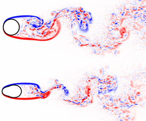
The mitigated wake meandering with the optimal shape can also be examined by the instantaneous spanwise vorticity. Figure 13 shows the instantaneous spanwise vorticity $\omega _z$ with a comparison between the initial and optimal cylinders. The maximum width of the first spanwise vortex is approximately $0.7$, located at approximately $x/D=1.6$. In contrast, the optimal shape leads to maximum width $0.58$ at approximately $x/D=1.4$, slightly less than for the initial shape. Notable differences can be observed at the third vortex further downstream. The initial shape leads to the maximum width of the third vortex being nearly $2.2$ at $x/D=8$, while the optimal shape provides that being $1.7$ at $x/D=6$. The reduced width of the shedding vortex leads to the weakened wake meandering, likely due to the alleviated Kelvin–Helmholtz (KH) instability that will be investigated in § 3.6.

Figure 13. Contours of instantaneous spanwise vorticity $\omega _z$, with comparison of (a) the circular cylinder and (b) the optimized shape.

3.5. Spectral analysis of turbulent wakes behind the optimal cylinder

We investigate the flow field of the optimal shape in the frequency domain based on the spectral analysis methods, including the single-point frequency spectrum and spectral proper orthogonal decomposition (POD) techniques (Sieber, Paschereit & Oberleithner Reference Sieber, Paschereit and Oberleithner2016; Schmidt et al. Reference Schmidt, Towne, Rigas, Colonius and Bres2018). The single-point frequency spectrum is used to investigate the frequency distribution of the velocity-fluctuating energy at different spatial locations. This is to identify the dominant frequency range at which the wake oscillation is mitigated significantly. Further, the spectral POD method is used to visualize the spatial modes at the leading frequency responsible for the wake mitigation.

The TKE is mitigated primarily in the large-scale, low-frequency flow structures. It is supported by the predicted power spectral density with the circular and optimized shapes. Figure 14 shows the energy spectrum of transverse velocity at spatial points $x/D=1, 3, 5, 7$ along the centreline. The spectral density is computed with the Welch method. At the point $x/D=1$, the magnitude of the spectral density is reduced at a wide bandwidth of frequency. That is probably because this sensor point is located close to the bluff body where the KH vortex rolls up and breaks down, fluctuating at various frequencies. The optimal shape reduces the velocity magnitude within the shear layer, which mitigates the formation and breakdown of the KH vortex and further velocity fluctuations at different scales. As the KH vortex evolves further downstream, e.g. at the location $x/D=5$, the spectral density with the optimized cylinder is similar to the baseline flow at high frequency, and the main difference between the two shapes lies in the low-frequency range. Given that, the optimal shape mainly reduces the velocity fluctuation of the large-scale flow structure at low frequencies compared to the flows over the baseline circular cylinder. Moreover, it is observed that the optimal shape reduces the magnitude of velocity-fluctuating energy while marginally increasing the leading frequency.

Figure 14. Single-point spectral density $\boldsymbol{\varPhi}_{vv}$ of the transverse velocity at different locations, i.e. $x/D=1, 3, 5, 7$, along the centreline downstream, with comparison between the circular and optimized shapes. Here, $D_c$ is the maximum diameter of the cylinder shape.

The spectral POD approach (Sieber et al. Reference Sieber, Paschereit and Oberleithner2016) is further used to investigate the large-scale coherent structures of the turbulent wake with the initial and optimized shapes. The method is the frequency-domain form of POD, which can characterize the leading frequency and corresponding dominant modes of the wake flows (Schmidt et al. Reference Schmidt, Towne, Rigas, Colonius and Bres2018). Readers are referred to Schmidt & Colonius (Reference Schmidt and Colonius2020) for details of the spectral POD method. We compare the frequency and the spatial mode with the optimal shape and the circular cylinder, as provided in figure 15. It can be seen that the leading frequency of wake flows behind the optimal cylinder is increased compared to that of the circular cylinder. Specifically, the leading frequency is $0.18$ for the circular cylinder, while that for the optimal shape is $0.26$. Although the optimal shape increases the leading frequency, the magnitude of the spectral POD eigenvalue is significantly reduced compared to the circular cylinder. Moreover, the optimal shape induces a narrower spatial mode than that of the initial cylinder, particularly in the far-wake region, as shown in figure 15. The spectral POD analysis further validates that the optimal shape mainly mitigates the velocity fluctuations of the large-scale flow structure in the wake flow.

Figure 15. (a,b) Spectral POD eigenvalue as a function of frequency, and (c,d) the mode at the leading frequency, with comparison between the circular and optimal shapes. Again, $D_c$ is the maximum diameter of the cylinder shape.

3.6. Mechanism of the turbulent wake mitigation

Here, we discuss briefly the mechanism of the turbulent wake mitigation with the optimal cylinder. The optimized shape is an asymmetric oval with the front part narrower than the rear part of the cylinder. Based on the predicted flow field, it is found that the flow field of the optimal cylinder increases the shedding frequency while reducing the wake-meandering amplitude. The increased shedding frequency is caused by the reduced diameter of the bluff body. Specifically, the KH frequency is inversely proportional to the momentum thickness of the shear layer (Prasad & Williamson Reference Prasad and Williamson1997), which can be scaled with the width of the bluff body (Bloor Reference Bloor1964). As such, the reduced cylinder width can decrease the shear layer thickness and further increase the frequency of the shedding vortex. We examine the thickness of the shear layer in figure 16(a). It shows that the shear layer thickness with the optimal shape is noticeably reduced compared to the baseline circular cylinder, which increases the vortex shedding frequency. The shear layer thickness is defined to be the transverse distance over which the mean velocity difference varies from $0.01\,\Delta U_m$ to $0.99\,\Delta U_m$, where $\Delta U_m$ is the mean velocity difference across the shear layer (Prasad & Williamson Reference Prasad and Williamson1997). On the other hand, the reduced wake-meandering amplitude is likely due to the mild curvature of the optimized shape, which reduces the velocity difference of the shear layer and alleviates the KH instability. This is supported in figure 16(b), explicitly showing the velocity difference between the wake centreline and mainstream with the optimal shape. The weaker velocity deficit of the optimal shape can be attributed to the favourable pressure gradient when compared with the baseline flow, as shown in figure 16(c). The experimental data of pressure coefficients (Norberg Reference Norberg1993) are also provided to validate the LES of the flow over the circular cylinder. The baseline cylinder has a relatively large favourable pressure gradient due to large curvature, accelerating the shear layer flows, and increasing velocity differences between the wake and the mainstream. Such large velocity differences can lead to strong KH instability and velocity fluctuations. In contrast, the optimal shape reduces the favourable pressure gradient with the mild curvature, which can alleviate the KH instability and the wake fluctuations by reducing the velocity difference between the wake and the mainstream flows.

Figure 16. Characteristics of the shear layer and the pressure coefficient over the azimuthal angle at the cylinder surface: (a) thickness of the shear layer; (b) velocity difference of the shear layer; (c) surface pressure coefficient.

4. Conclusion

This work introduces the regularized ensemble Kalman method for LES-based shape optimization. The shape of a bluff body is optimized to minimize the TKE in the near-wake region. The LES are used to predict the velocity fluctuations given the shape variations. Within the ensemble Kalman method, the ensemble-based sensitivity analysis is used to compute the gradient of the LES-based TKE prediction with respect to the geometric parameters to guide the optimization process. Such gradients are estimated based on sample statistics of geometric parameters and LES predictions, which circumvents the blowup issue of the conventional adjoint-based gradient for turbulent flows. Moreover, the smoothness regularization is imposed based on the regularized ensemble Kalman method to avoid large variations of the optimized shape.

The feasibility of the ensemble-based sensitivity for the chaotic problem is first assessed in the Lorenz system. Our results examine the accuracy of the ensemble-based gradient, which effectively avoids the blowup issue of the adjoint-based sensitivity and provides usable gradients for optimization of chaotic systems with small sample sizes. Further, we demonstrate the capability of the regularized ensemble Kalman method in optimizing the cylinder shape based on LES to mitigate the turbulent fluctuation of wake flows. With the method, the cylinder is optimized to be an asymmetric oval with the width of the rear part larger than the front. By analysing the flow field between the optimal and baseline circular shapes, we observe that the optimal shape mitigates the turbulent fluctuations mainly from the large-scale flow structure. This is achieved by reducing the velocity difference of the shear layer with a mild curvature of the optimized shape. This mitigates the shear layer and KH instability, resulting in the reduced magnitude of wake meandering.

The ensemble-based sensitivity is feasible for the LES-based optimization and could be extended to data-driven subgrid stress modelling (MacArt, Sirignano & Freund Reference MacArt, Sirignano and Freund2021; Novati, de Laroussilhe & Koumoutsakos Reference Novati, de Laroussilhe and Koumoutsakos2021) and wall modelling (Bae & Koumoutsakos Reference Bae and Koumoutsakos2022). However, the ensemble-based sensitivity analysis relies on the sample statistics and tends to encounter sample collapse issues due to limited sample sizes. That is, the samples converge around the sample mean, which underestimates sample variance and leads to negligible model gradients. For this reason, the inflation technique may be introduced to alleviate the sampling errors. On the other hand, the ensemble method requires running multiple LES to compute the gradient, which would hinder the application to complex flow scenarios with high Reynolds numbers. Efficient computation of the ensemble-based gradient is worthy of further investigation.

Acknowledgements

The authors thank the reviewers for their constructive and valuable comments, which greatly improved the quality and clarity of this paper.

Funding

This work is supported by the NSFC Basic Science Center Program for ‘Multiscale problems in nonlinear mechanics’ (no. 11988102). X.-L.Z. also acknowledges support from the National Natural Science Foundation of China (no. 12102435) and the Young Elite Scientists Sponsorship Program by CAST (no. 2022QNRC001).

Declaration of interests

The authors report no conflict of interest.

Appendix A. Procedure of the ensemble Kalman method for shape optimization

Given the baseline geometric parameters, the standard deviation $\sigma _a$ of the initial sample distribution, and the weight parameter ${R}$, the cylinder shape can be optimized by following the procedure below.

  1. (i) Initial sampling. The samples of geometric parameters are drawn randomly around the baseline geometric parameters based on the given standard deviation $\sigma _a$. The normal distribution is considered for each geometric parameter in this work.

  2. (ii) Imposing constraints. The geometric parameter $\boldsymbol {a}$ is constrained to meet prescribed requirements to have a fixed volume and physically well-defined geometry. Further, the obtained geometric parameters are regularized to enforce smoothness with the regularization step based on (2.19a), (2.21) and (2.22).

  3. (iii) Geometric generation. Each sample of the geometric parameter is used to generate the geometry of bluff bodies by combining with the Fourier bases based on (2.6) and (2.7a,b).

  4. (iv) The LES-based propagation. For each geometry, the LES are performed to evaluate the spatial-averaged TKE in the prescribed wake region based on (2.4).

  5. (v) Ensemble-based sensitivity. The covariance between the geometric parameter and the predicted TKE is used to evaluate the model gradient with respect to the geometric parameters based on (2.13).

  6. (vi) Kalman-based update. Based on the model prediction, the ensemble-based gradient and Hessian of the cost function can be obtained, which is used to update the geometric parameters as (2.19b).

The iteration is stopped when the TKE reduces below the noise level based on the discrepancy principle (Ernst, Sprungk & Starkloff Reference Ernst, Sprungk and Starkloff2015) or the maximum iteration number is reached. The procedure of the ensemble-based shape optimization is illustrated schematically in figure 17.

Figure 17. Schematic of ensemble-based shape optimization for mitigation of wake turbulence: (a) generate initial samples of geometric parameters; (b) impose hard and soft constraints; (c) generate cylinder shapes given geometric parameters; (d) predict the TKE in the wake region based on LES; (e) compute the ensemble-based sensitivity; (f) update the geometric parameters based on the ensemble Kalman scheme.

Appendix B. Sensitivity study of sample sizes for the Lorenz system

In this Appendix, we test the effects of the sample sizes on the accuracy of the ensemble-based gradient for the Lorenz system. The gradient $\textrm {d} \langle z \rangle / \textrm {d} \rho$ is estimated with the ensemble-based sensitivity analysis approach. Different sample sizes, including $10$, $100$ and $1000$, are tested. The estimated ensemble-based gradient at different values of the parameter $\rho$ is shown in figure 18. It can be seen that for $\rho < 23$, the gradients are similar with different ensemble sizes, because the Lorenz system is a fixed-point attractor at this parameter range, which allows very small ensemble sizes, e.g. $10$, to capture the linear mapping between the parameter $\rho$ and the output $\langle z \rangle$. For $\rho >24.5$, the estimated gradient with sample size $10$ becomes unsmooth and oscillates around $1$. Increasing the sample size to $100$, the ensemble-based sensitivity can alleviate the oscillations and provide relatively accurate gradients for each parameter $\rho$. With sample size $1000$, the estimated gradient can be very close to the reference even in the chaotic regime.

Figure 18. The ensemble-based gradient $\textrm {d} \langle z \rangle / \textrm {d} \rho$ for the parameters $\rho \in [0, 50]$ with different sample sizes for the Lorenz system: (a) $M = 10$, (b) $M = 100$ and (c) $M = 1000$.

References

Ancell, B. & Hakim, G.J. 2007 Comparing adjoint- and ensemble-sensitivity analysis with applications to observation targeting. Mon. Weath. Rev. 135 (12), 41174134.CrossRefGoogle Scholar
Bae, H.J. & Koumoutsakos, P. 2022 Scientific multi-agent reinforcement learning for wall-models of turbulent flows. Nat. Commun. 13 (1), 1443.CrossRefGoogle ScholarPubMed
Blonigan, P.J., Fernandez, P., Murman, S.M., Wang, Q., Rigas, G. & Magri, L. 2016 Toward a chaotic adjoint for LES. In Proceedings of the Summer Program, Center for Turbulence Research, Stanford University.Google Scholar
Bloor, M.S. 1964 The transition to turbulence in the wake of a circular cylinder. J. Fluid Mech. 19 (2), 290304.CrossRefGoogle Scholar
Bodony, D.J. & Lele, S.K. 2005 On using large-eddy simulation for the prediction of noise from cold and heated turbulent jets. Phys. Fluids 17 (8), 085103.Google Scholar
Cattafesta, L.N. III & Sheplak, M. 2011 Actuators for active flow control. Annu. Rev. Fluid Mech. 43, 247272.CrossRefGoogle Scholar
Chandramoorthy, N., Fernandez, P., Talnikar, C. & Wang, Q. 2019 Feasibility analysis of ensemble sensitivity computation in turbulent flows. AIAA J. 57 (10), 45144526.CrossRefGoogle Scholar
Chen, Y., Oliver, D.S. & Zhang, D. 2009 Efficient ensemble-based closed-loop production optimization. SPE J. 14 (4), 634645.CrossRefGoogle Scholar
Choi, H., Jeon, W.-P. & Kim, J. 2008 Control of flow over a bluff body. Annu. Rev. Fluid Mech. 40, 113139.CrossRefGoogle Scholar
Colburn, C.H., Cessna, J.B. & Bewley, T.R. 2011 State estimation in wall-bounded flow systems. Part 3. The ensemble Kalman filter. J. Fluid Mech. 682, 289303.CrossRefGoogle Scholar
Dhert, T., Ashuri, T. & Martins, J.R.R.A. 2017 Aerodynamic shape optimization of wind turbine blades using a Reynolds-averaged Navier–Stokes model and an adjoint method. Wind Energy 20 (5), 909926.CrossRefGoogle Scholar
Ernst, O.G., Sprungk, B. & Starkloff, H.-J. 2015 Analysis of the ensemble and polynomial chaos Kalman filters in Bayesian inverse problems. SIAM/ASA J. Uncertainty Quant. 3 (1), 823851.CrossRefGoogle Scholar
Evensen, G. 2009 Data Assimilation: The Ensemble Kalman Filter. Springer.CrossRefGoogle Scholar
Evensen, G. 2018 Analysis of iterative ensemble smoothers for solving inverse problems. Comput. Geosci. 22 (3), 885908.CrossRefGoogle Scholar
Ge, L. & Sotiropoulos, F. 2007 A numerical method for solving the 3D unsteady incompressible Navier–Stokes equations in curvilinear domains with complex immersed boundaries. J. Comput. Phys. 225 (2), 17821809.CrossRefGoogle ScholarPubMed
Germano, M., Piomelli, U., Moin, P. & Cabot, W.H. 1991 A dynamic subgrid-scale eddy viscosity model. Phys. Fluids A: Fluid Dyn. 3 (7), 17601765.CrossRefGoogle Scholar
Gilmanov, A. & Sotiropoulos, F. 2005 A hybrid Cartesian/immersed boundary method for simulating flows with 3D, geometrically complex, moving bodies. J. Comput. Phys. 207 (2), 457492.CrossRefGoogle Scholar
Holst, T. & Pulliam, T. 2001 Aerodynamic shape optimization using a real-number-encoded genetic algorithm. In 19th AIAA Applied Aerodynamics Conference, 2001-2473.Google Scholar
Huang, D.Z., Schneider, T. & Stuart, A.M. 2022 Iterated Kalman methodology for inverse problems. J. Comput. Phys. 463, 111262.CrossRefGoogle Scholar
Hunt, B.R., Kostelich, E.J. & Szunyogh, I. 2007 Efficient data assimilation for spatiotemporal chaos: a local ensemble transform Kalman filter. Phys. D: Nonlinear Phenom. 230 (1–2), 112126.CrossRefGoogle Scholar
Iglesias, M.A., Law, K.J.H. & Stuart, A.M. 2013 Ensemble Kalman methods for inverse problems. Inverse Probl. 29 (4), 045001.CrossRefGoogle Scholar
Jahanbakhshi, R. & Zaki, T.A. 2023 Optimal two-dimensional roughness for transition delay in high-speed boundary layer. J. Fluid Mech. 968, A24.CrossRefGoogle Scholar
Kiefer, J. & Wolfowitz, J. 1952 Stochastic estimation of the maximum of a regression function. Ann. Math. Stat. 23 (3), 462466.CrossRefGoogle Scholar
Knoll, D.A. & Keyes, D.E. 2004 Jacobian-free Newton–Krylov methods: a survey of approaches and applications. J. Comput. Phys. 193 (2), 357397.CrossRefGoogle Scholar
Kovachki, N.B. & Stuart, A.M. 2019 Ensemble Kalman inversion: a derivative-free technique for machine learning tasks. Inverse Probl. 35 (9), 095005.CrossRefGoogle Scholar
Labahn, J.W., Wu, H., Harris, S.R., Coriton, B., Frank, J.H. & Ihme, M. 2020 Ensemble Kalman filter for assimilating experimental data into large-eddy simulations of turbulent flows. Flow Turbul. Combust. 104, 861893.CrossRefGoogle Scholar
Lai, T.L. 2003 Stochastic approximation. Ann. Stat. 31 (2), 391406.CrossRefGoogle Scholar
Lea, D.J., Allen, M.R. & Haine, T.W.N. 2000 Sensitivity analysis of the climate of a chaotic system. Tellus A: Dyn. Meteorol. Oceanogr. 52 (5), 523532.CrossRefGoogle Scholar
Li, G. & Reynolds, A.C. 2011 Uncertainty quantification of reservoir performance predictions using a stochastic optimization algorithm. Comput. Geosci. 15, 451462.CrossRefGoogle Scholar
Lorente-Macias, J., Bengana, Y. & Hwang, Y. 2023 Shape optimisation for a stochastic two-dimensional cylinder wake using ensemble variation. J. Fluid Mech. 959, A7.CrossRefGoogle Scholar
Luo, X. 2021 Novel iterative ensemble smoothers derived from a class of generalized cost functions. Comput. Geosci. 25 (3), 11591189.CrossRefGoogle Scholar
MacArt, J.F., Sirignano, J. & Freund, J.B. 2021 Embedded training of neural-network subgrid-scale turbulence models. Phys. Rev. Fluids 6 (5), 050502.CrossRefGoogle Scholar
Mani, K. & Mavriplis, D.J. 2008 Unsteady discrete adjoint formulation for two-dimensional flow problems with deforming meshes. AIAA J. 46 (6), 13511364.CrossRefGoogle Scholar
Marsden, A.L., Wang, M., Dennis, J.E. & Moin, P. 2007 Trailing-edge noise reduction using derivative-free optimization and large-eddy simulation. J. Fluid Mech. 572, 1336.CrossRefGoogle Scholar
Michelén-Ströfer, C.A., Zhang, X.-L. & Xiao, H. 2021 a DAFI: an open-source framework for ensemble-based data assimilation and field inversion. Commun. Comput. Phys. 29 (5), 15831622.CrossRefGoogle Scholar
Michelén-Ströfer, C.A., Zhang, X.-L. & Xiao, H. 2021 b Ensemble gradient for learning turbulence models from indirect observations. Commun. Comput. Phys. 30 (5), 12691292.CrossRefGoogle Scholar
Min, C. & Choi, H. 1999 Suboptimal feedback control of vortex shedding at low Reynolds numbers. J. Fluid Mech. 401, 123156.CrossRefGoogle Scholar
Mohammadi, B. & Pironneau, O. 2009 Applied Shape Optimization for Fluids. Oxford University Press.CrossRefGoogle Scholar
Moldovan, G., Lehnasch, G., Cordier, L. & Meldi, M. 2021 A multigrid/ensemble Kalman filter strategy for assimilation of unsteady flows. J. Comput. Phys. 443, 110481.CrossRefGoogle Scholar
Mons, V., Du, Y. & Zaki, T.A. 2021 Ensemble-variational assimilation of statistical data in large-eddy simulation. Phys. Rev. Fluids 6 (10), 104607.CrossRefGoogle Scholar
Nadarajah, S.K. & Jameson, A. 2007 Optimum shape design for unsteady flows with time-accurate continuous and discrete adjoint method. AIAA J. 45 (7), 14781491.CrossRefGoogle Scholar
Ni, A. & Wang, Q. 2017 Sensitivity analysis on chaotic dynamical systems by non-intrusive least squares shadowing (NILSS). J. Comput. Phys. 347, 5677.CrossRefGoogle Scholar
Norberg, C. 1993 Pressure forces on a circular cylinder in cross flow. In Bluff-Body Wakes, Dynamics and Instabilities: IUTAM Symposium, Göttingen, Germany September 7–11, 1992, pp. 275–278. Springer.CrossRefGoogle Scholar
Novati, G., de Laroussilhe, H.L. & Koumoutsakos, P. 2021 Automating turbulence modelling by multi-agent reinforcement learning. Nat. Mach. Intell. 3 (1), 8796.CrossRefGoogle Scholar
Parnaudeau, P., Carlier, J., Heitz, D. & Lamballais, E. 2008 Experimental and numerical studies of the flow over a circular cylinder at Reynolds number 3900. Phys. Fluids 20 (8), 085101.CrossRefGoogle Scholar
Patnaik, B.S.V. & Wei, G.W. 2002 Controlling wake turbulence. Phys. Rev. Lett. 88 (5), 054502.CrossRefGoogle ScholarPubMed
Prasad, A. & Williamson, C.H.K. 1997 The instability of the shear layer separating from a bluff body. J. Fluid Mech. 333, 375402.CrossRefGoogle Scholar
Rackauckas, C. & Nie, Q. 2017 DifferentialEquations.jl – a performant and feature-rich ecosystem for solving differential equations in Julia. J. Open Res. Softw. 5 (1), 15.CrossRefGoogle Scholar
Rashidi, S., Hayatdavoodi, M. & Esfahani, J.A. 2016 Vortex shedding suppression and wake control: a review. Ocean Engng 126, 5780.CrossRefGoogle Scholar
Saad, Y. 1993 A flexible inner–outer preconditioned GMRES algorithm. SIAM J. Sci. Comput. 14 (2), 461469.CrossRefGoogle Scholar
Schillings, C. & Stuart, A.M. 2017 Analysis of the ensemble Kalman filter for inverse problems. SIAM J. Numer. Anal. 55 (3), 12641290.CrossRefGoogle Scholar
Schmidt, O.T. & Colonius, T. 2020 Guide to spectral proper orthogonal decomposition. AIAA J. 58 (3), 10231033.CrossRefGoogle Scholar
Schmidt, O.T., Towne, A., Rigas, G., Colonius, T. & Bres, G.A. 2018 Spectral analysis of jet turbulence. J. Fluid Mech. 855, 953982.CrossRefGoogle Scholar
Schneider, T., Stuart, A.M. & Wu, J.-L. 2022 Ensemble Kalman inversion for sparse learning of dynamical systems from time-averaged data. J. Comput. Phys. 470, 111559.CrossRefGoogle Scholar
Sieber, M., Paschereit, C.O. & Oberleithner, K. 2016 Spectral proper orthogonal decomposition. J. Fluid Mech. 792, 798828.CrossRefGoogle Scholar
Smagorinsky, J. 1963 General circulation experiments with the primitive equations: I. The basic experiment. Mon. Weath. Rev. 91 (3), 99164.2.3.CO;2>CrossRefGoogle Scholar
Spall, J.C. 1992 Multivariate stochastic approximation using a simultaneous perturbation gradient approximation. IEEE Trans. Autom. Control 37 (3), 332341.CrossRefGoogle Scholar
Strogatz, S.H. 2018 Nonlinear Dynamics and Chaos: With Applications to Physics, Biology, Chemistry, and Engineering. CRC Press.CrossRefGoogle Scholar
Torn, R.D. & Hakim, G.J. 2008 Ensemble-based sensitivity analysis. Mon. Weath. Rev. 136 (2), 663677.CrossRefGoogle Scholar
Wang, Q., Hu, R. & Blonigan, P. 2014 Least squares shadowing sensitivity analysis of chaotic limit cycle oscillations. J. Comput. Phys. 267, 210224.CrossRefGoogle Scholar
Wang, Q., Moin, P. & Iaccarino, G. 2009 Minimal repetition dynamic checkpointing algorithm for unsteady adjoint calculation. SIAM J. Sci. Comput. 31 (4), 25492567.CrossRefGoogle Scholar
Xiao, H. & Cinnella, P. 2019 Quantification of model uncertainty in RANS simulations: a review. Prog. Aerosp. Sci. 108, 131.CrossRefGoogle Scholar
Yang, X., Sotiropoulos, F., Conzemius, R.J., Wachtler, J.N. & Strong, M.B. 2015 Large-eddy simulation of turbulent flow past wind turbines/farms: the virtual wind simulator (VWIS). Wind Energy 18 (12), 20252045.CrossRefGoogle Scholar
Zhang, X.-L., Michelén-Ströfer, C. & Xiao, H. 2020 Regularized ensemble Kalman methods for inverse problems. J. Comput. Phys. 416, 109517.CrossRefGoogle Scholar
Zhang, X.-L., Xiao, H. & He, G. 2022 a Assessment of regularized ensemble Kalman method for inversion of turbulence quantity fields. AIAA J. 60 (1), 313.Google Scholar
Zhang, X.-L., Xiao, H., Luo, X. & He, G. 2022 b Ensemble Kalman method for learning turbulence models from indirect observation data. J. Fluid Mech. 949, A26.CrossRefGoogle Scholar
Zhang, X.-L., Zhang, L. & He, G. 2024 Parallel ensemble Kalman method with total variation regularization for large-scale field inversion. J. Comput. Phys. 509, 113059.CrossRefGoogle Scholar
Zhou, Z., Li, Z., He, G. & Yang, X. 2022 Towards multi-fidelity simulation of flows around an underwater vehicle with appendages and propeller. Theor. Appl. Mech. Lett. 12, 100318.CrossRefGoogle Scholar
Zhu, L., Wu, T. & He, G. 2022 Large-eddy simulation for the aero-vibro-acoustic analysis: plate–cavity system excited by turbulent channel flow. Acta Mechanica Sin. 38 (10), 322019.CrossRefGoogle Scholar
Figure 0

Figure 1. The results of the ensemble-based sensitivity analysis for the Lorenz system. (a) The state trajectory $z(t)$ with different parameters $\rho$. (b) The evolution of the time-averaged output $\langle z \rangle$ with the parameter $\rho$. The attractors with different parameters $\rho$ are also plotted. (c,d) The estimated gradients $\textrm {d} \langle z \rangle /\textrm {d}\rho$ with the adjoint and ensemble-based sensitivity analysis methods, respectively. The red circles in panel (d) indicate the gradient calculated by finite difference with the interval $\Delta \rho = 1$.

Figure 1

Figure 2. (a) Computational domain and (b) mesh refinement for LES of turbulent wakes behind the bluff body. The orange box indicates the region for calculating the spatial-averaged TKE in the wake. The grey and green boxes indicate the regions for mesh refinement with different resolutions.

Figure 2

Figure 3. Validation of the LES for turbulent flows over a circular cylinder at $Re=3900$.

Figure 3

Figure 4. Convergence of the cost function and TKE $K$ ($\lambda = 10$, $N=50$) in the convergence history for $0 \le i < 10$. The obtained shapes at iteration steps $i=0, 2, 4, 9$ are plotted alongside.

Figure 4

Figure 5. Optimal cylinder shape for different values of the regularization parameter $\lambda$ ($N=50$) and the corresponding prediction of TKE: (a) shape versus $\lambda$, and (b) $K$ versus $\lambda$.

Figure 5

Figure 6. Optimal cylinder shape for different numbers of the Fourier modes $N$ ($\lambda =10$) and the corresponding predictions of TKE: (a) shape versus $N$, and (b) $K$ versus $N$.

Figure 6

Figure 7. Optimal cylinder shape for different initial shapes and the corresponding predictions of TKE fields. The baseline indicates the optimized shape with the circular cylinder as the initial shape.

Figure 7

Figure 8. Optimal cylinder shape for different Reynolds numbers, and the corresponding predictions of TKE fields.

Figure 8

Figure 9. Comparison of (ac) the circular shape and (df) the optimized shape in the predicted TKE and Reynolds normal stresses.

Figure 9

Figure 10. Contour plots of the circular cylinder and optimized shape in (a,b) the predicted mean streamwise velocity and (c,d) the vertical velocity. The white line indicates the separation region.

Figure 10

Figure 11. Plots of TKE and streamwise velocity difference $\Delta U = \bar {u} - U_b$ along profiles, with comparison between the baseline circular cylinder and the optimal oval.

Figure 11

Figure 12. The standard deviation of the wake centreline, with comparison between the initial and optimized cylinders.

Figure 12

Figure 13. Contours of instantaneous spanwise vorticity $\omega _z$, with comparison of (a) the circular cylinder and (b) the optimized shape.

Figure 13

Figure 14. Single-point spectral density $\boldsymbol{\varPhi}_{vv}$ of the transverse velocity at different locations, i.e. $x/D=1, 3, 5, 7$, along the centreline downstream, with comparison between the circular and optimized shapes. Here, $D_c$ is the maximum diameter of the cylinder shape.

Figure 14

Figure 15. (a,b) Spectral POD eigenvalue as a function of frequency, and (c,d) the mode at the leading frequency, with comparison between the circular and optimal shapes. Again, $D_c$ is the maximum diameter of the cylinder shape.

Figure 15

Figure 16. Characteristics of the shear layer and the pressure coefficient over the azimuthal angle at the cylinder surface: (a) thickness of the shear layer; (b) velocity difference of the shear layer; (c) surface pressure coefficient.

Figure 16

Figure 17. Schematic of ensemble-based shape optimization for mitigation of wake turbulence: (a) generate initial samples of geometric parameters; (b) impose hard and soft constraints; (c) generate cylinder shapes given geometric parameters; (d) predict the TKE in the wake region based on LES; (e) compute the ensemble-based sensitivity; (f) update the geometric parameters based on the ensemble Kalman scheme.

Figure 17

Figure 18. The ensemble-based gradient $\textrm {d} \langle z \rangle / \textrm {d} \rho$ for the parameters $\rho \in [0, 50]$ with different sample sizes for the Lorenz system: (a) $M = 10$, (b) $M = 100$ and (c) $M = 1000$.